A line-binned treatment of opacities for the spectra and
light curves from neutron star mergers

Abstract

The electromagnetic observations of GW170817 were able to dramatically increase our understanding of neutron star mergers beyond what we learned from gravitational waves alone. These observations provided insight on all aspects of the merger from the nature of the gamma-ray burst to the characteristics of the ejected material. The ejecta of neutron star mergers are expected to produce such electromagnetic transients, called kilonovae or macronovae. Characteristics of the ejecta include large velocity gradients, relative to supernovae, and the presence of heavy $r$-process elements, which pose significant challenges to the accurate calculation of radiative opacities and radiation transport. For example, these opacities include a dense forest of bound-bound features arising from near-neutral lanthanide and actinide elements. Here we investigate the use of fine-structure, line-binned opacities that preserve the integral of the opacity over frequency. Advantages of this area-preserving approach over the traditional expansion-opacity formalism include the ability to pre-calculate opacity tables that are independent of the type of hydrodynamic expansion and that eliminate the computational expense of calculating opacities within radiation-transport simulations. Tabular opacities are generated for all 14 lanthanides as well as a representative actinide element, uranium. We demonstrate that spectral simulations produced with the line-binned opacities agree well with results produced with the more accurate continuous Monte Carlo Sobolev approach, as well as with the commonly used expansion-opacity formalism. Additional investigations illustrate the convergence of opacity with respect to the number of included lines, and elucidate sensitivities to different atomic physics approximations, such as fully and semi-relativistic approaches.

1 Introduction

The merger of two neutron stars has been proposed both as the source of short-duration gamma-ray bursts (Narayan et al., 1992) and the site of $r$-process production (Symbalisty & Schramm, 1982). Simulations confirmed that the neutron-rich, dynamical ejecta from neutron star mergers (NSMs) robustly produced $r$-process elements from the second through third $r$-process peaks (Rosswog et al., 1999, 2014; Just et al., 2015). With the gravitational wave (Abbott et al., 2017a) and subsequent follow-up observations in the electromagnetic spectrum (Abbott et al., 2017b) of a nearby merger event, astronomers were able, for the first time, to validate these theories and, to some extent, determine the yields from these NSMs.

On the surface, the light curves and spectra seem to be a validation of the ejecta predicted by the merger simulations. Theorists had proposed a two-component model for the ejecta consisting of a neutron-rich dynamical ejecta (producing heavy $r$-process elements) and a higher electron fraction wind ejecta (light $r$-process and iron peak elements) (Metzger & Berger, 2012; Metzger, 2017). A significant number of lanthanide and actinide elements are predicted to be present in the ejecta (see, for example, Figure 1).

Figure 1: Predicted elemental abundances for the ejecta produced in a $1.4+1.4\,{\rm M_{\odot}}$ neutron star merger (Rosswog et al., 2014; Grossman et al., 2014), approximately one day after merger. A few labels are provided for easy identification of various lanthanide and actinide elements considered in this work.

The high opacities associated with these elements produced in the heavy $r$-process support an argument for late-time, infra-red emission, whereas the wind ejecta would produce early-time UV/optical emission. With observations of both an early UV/optical and later infra-red emission, astronomers could place constraints on the amount of ejecta in each component. Many groups attempted such studies, producing a wide range of results (for a review, see Côté et al., 2017) and, although all agree that roughly $0.01$ M_⊙ was ejected in the merger, the exact amount and the exact composition of the ejecta still remains a subject of debate.

The differences in the yield predictions arise from different assumptions in the structure of the ejecta, the composition of the ejecta and the opacities. In many simulations, the ejecta was modeled in spherical symmetry. By varying the velocity, mass and composition of the ejecta, these models produce a range of emission spectra that can be combined to form multi-component models (Pian et al., 2017; Cowperthwaite et al., 2017). Multi-dimensional models can include more detailed ejecta profiles. For example, a set of models included two-component ejecta properties with the dynamical, heavy $r$-process rich ejecta driven along the orbital plane and a more spherical wind ejecta (Tanvir et al., 2017; Troja et al., 2017; Kasen et al., 2017; Wollaeger et al., 2018; Tanaka et al., 2018). These structures can produce different emission properties for the same production rate of heavy $r$-process elements. Additionally, even for the same model morphology, there remain differences in the light-curve predictions from the various modeling groups. For example, a major difference is a redward shift in the peak emission produced by different groups. We discuss this shift in Section 4.2 and show that this behavior is not due to the different ways in which the opacities are implemented in the radiation-transport simulations.

The range of opacities used also varies dramatically. Many models rely on constant opacity values, varying from 0.2 to 30 cm²/g. Only a few models used detailed, frequency-dependent opacities based on atomic physics calculations and these calculations are still limited to a few lanthanide elements used as surrogates for the heavy $r$-process elements (Barnes et al., 2016; Kasen et al., 2017; Wollaeger et al., 2018; Tanaka et al., 2018). Calculating accurate opacities for lanthanides and actinides pushes the frontier in atomic physics research due to the complexity in modeling the interaction of many bound electrons, some of which occupy a partially filled $f$ shell. Generating a complete set of opacities requires making approximations in the atomic physics calculations that can significantly alter NSM spectral simulations.

In addition, the implementation of these opacities in NSM modeling also varies from group to group. Due to the existence of a strong velocity gradient in the ejecta, Doppler effects must be included in the opacities. This requirement typically includes both a correction to the optical depth of each line (Sobolev, 1960) and effects on line broadening, leading to a variety of expansion-opacity approaches (Castor, 2004). These methods require line lists that can be difficult to include in their entirety in light-curve calculations due to the large number of lines associated with lanthanide and actinide elements. In this work, we propose using precomputed, binned line contributions, which allows opacities to be generated in a compact tabular form for convenient use in transport calculations. This line-binned approach is guaranteed to preserve the integral of the opacity over frequency and supersedes our earlier, preliminary attempt to achieve this goal using line-smeared opacities.

This paper presents a first set of lanthanide opacities, as well as a representative actinide (uranium) opacity, to be used in light-curve calculations for NSMs. In Section 2 we review the methods and some of the uncertainties in the atomic physics calculations for these heavy opacities, discussing relevant approximations, such as semi- versus fully relativistic models and configuration interaction. In Section 3 we present a range of line-binned opacities for NSM calculations, illustrating similarities and differences in the lanthanide and uranium opacities. Motivation and justification for our line-binned opacity approach is presented in Section 4. We summarize with a brief discussion of the implications of our results for observations.

2 Atomic Physics Considerations

2.1 Computational Framework

In this work we use the Los Alamos suite of atomic physics and plasma modeling codes (see Fontes et al. 2015b and references therein) to generate the fundamental data and opacities needed to simulate the characteristics (time to peak, spectra, luminosities, decay times, etc.) associated with neutron star mergers. For a given element, a model is composed of the atomic structure (energies, wavefunctions and oscillator strengths) and photoionization cross sections. Both the fully and semi-relativistic capabilities of the suite are used in this work.

The fully relativistic (FR) approach is based on bound- and continuum-electron wavefunctions that are solutions of the Dirac equation, while the semi-relativistic (SR) approach uses solutions of the Schrödinger equation with relativistic corrections. A fully relativistic (FR) calculation begins with the RATS atomic structure code (Fontes et al., 2015b) using the Dirac-Fock-Slater method of Sampson and co-workers (Sampson et al., 2009). A semi-relativistic (SR) calculation begins with the CATS atomic structure code (Abdallah et al., 1988) using the Hartree-Fock method of Cowan (Cowan, 1981). These calculations produce detailed, fine-structure data that include a complete description of configuration interaction for the specified list of configurations. Two variant, relativistic calculations are also considered that include incomplete amounts of configuration interaction (see Section 2.2). After the atomic structure calculations are complete, both the FR and SR methods use the GIPPER ionization code to obtain the relevant photoionization cross sections in the distorted-wave approximation. The photoionization data are used to generate the bound-free contribution to the opacity and are not expected to be too important for the present application, due to the range of relevant photon energies, but are included for completeness. Therefore, they are calculated in the configuration-average approximation, rather than fine-structure detail, in order to minimize the computational time.

The atomic level populations are calculated with the ATOMIC code from the fundamental atomic data. The code can be used in either local thermodynamic equilibrium (LTE) or non-LTE mode (Magee et al., 2004; Hakel & Kilcrease, 2004; Hakel et al., 2006; Colgan et al., 2016; Fontes et al., 2016). The LTE approach was chosen for the present application, which requires only the atomic structure data in calculating the populations. At the relevant times, the ejecta densities are low enough that collective, or plasma, effects are not important and simple Saha-Boltzmann statistics is sufficient to produce accurate level populations. The populations are then combined with the oscillator strengths and photoionization cross sections in ATOMIC to obtain the monochromatic opacities, which are constructed from the standard four contributions: bound-bound (b-b), bound-free (b-f), free-free (f-f) and scattering. Specific formulae for these contributions are readily available in various textbooks, such as Huebner & Barfield (2014).

Here, we reproduce only the expression for the bound-bound contribution, as it is useful in understanding the subsequent expression for line-binned opacities, as well as the discussion of such quantities in Section 3:

$$\kappa^{\rm b-b}_{\nu}=\frac{\pi e^{2}}{\rho m_{e}c}\sum_{i}N_{i}\,|f_{i}|\,L_{i,\nu}\,,$$ (1)

where $\nu$ is the photon energy, $\rho$ is the mass density, $N_{i}$ is the number density of the initial level in transition $i$, $f_{i}$ is the oscillator strength describing the photo-excitation of transition $i$, and $L_{i,\nu}$ is the corresponding line profile function. The line-binned opacities proposed in this work are comprised of discrete frequency (or wavelength) bins that contain a sum over all of the lines centered within a bin. An expression for this discrete opacity is obtained from the continuous opacity displayed in Equation (1) by replacing the line profile with $1/\Delta\nu_{j}$, i.e.

$$\kappa^{\rm bin}_{\nu,j}=\frac{1}{\Delta\nu_{j}}\frac{\pi e^{2}}{\rho m_{e}c}\sum_{i\in\Delta\nu_{j}}N_{i}\,|f_{i}|\,,$$ (2)

where $\Delta\nu_{j}$ represents the frequency width of a bin denoted by integer index $j$. So, the summation encompasses all lines $i$ with centers that reside in bin $j$. It is straightforward to show that numerical integration of Equation (2) over all bins produces the same value as that obtained by analytically integrating Equation (1) because the line profile function is normalized to one when integrating over all frequencies. The form of Equation (1) is clearly independent of the type of expansion, which is a distinct advantage over methods that assume a homologous flow, such as the expansion-opacity approach. However, the line-binned opacities are expected to be significantly different than those produced with more traditional approaches. Physical arguments and numerical examples in support of using these line-binned, area-preserving opacities to model kilonovae is provided in Section 4.

The line-binned opacities in Equation (2) can be readily cast in a tabular form, using a discrete temperature/mass-density grid, that is commonly employed in radiation-hydrodynamics simulations. In the latter approach, discrete photon frequency groups are chosen to model the flow of radiation, and the groups are typically much less resolved compared to the frequency bins. If a particular group is denoted by integer index $g$, and the group boundaries exactly align with specific bin boundaries, then (unweighted) group opacities can be computed in a straightforward manner from Equation (2) via the formula

$$\kappa^{\rm group}_{\nu,g}=\frac{1}{\Delta\nu_{g}}\sum_{j\in\Delta\nu_{g}}\Delta\nu_{j}\,\kappa^{\rm bin}_{\nu,j}\,,$$ (3)

where $\Delta\nu_{g}$ is the frequency width of group $g$. If a bin overlaps with more than one group, its opacity contribution is distributed across those groups in proportion to the area in each group.

When constructing opacity tables, a practical consideration involves the choice of an oscillator strength cutoff value, which we denote by $f_{c}$. Rather than evalutating the summation in Equation (2) over all available lines, we consider only lines with an oscillator strength above some prescribed value. For the conditions of interest for modeling kilonovae, we found that a value of $f_{c}=10^{-6}$ is typically sufficient to produce converged results. Unless otherwise noted, this cutoff value was used when constructing all of the opacity data discussed in this work.

2.2 Baseline Atomic Models

As mentioned in Section 1, atomic models were created for all 14 lanthanides and one representative actinide (uranium). In order to obtain converged opacities for the range of temperatures and densities in our simulations, only the first four ion stages of each element were considered, similar to the choice made by Kasen et al. (2013). A list of configurations chosen for each element is provided in Table 4 of Appendix A. Since Nd was used as a representative element in the recent study by Kasen et al. (2013), we chose an identical list of configurations for that element in order to make meaningful comparisons. As expected, the number of Nd levels is identical to those appearing in Table 1 of that earlier work. The number of lines is slightly higher in the present listing, possibly due to the retention of small oscillator strengths that do not affect the modeling in a significant way. We did some tests to include higher lying configurations, but found that the displayed list is sufficient to produce converged opacities due to the relatively low temperature and densities of the ejecta. Therefore, the configuration lists for the other elements were chosen in a similar fashion. The configurations for Ce ii and Ce iii are also identical to those chosen by Kasen et al. (2013). The number of levels and lines differ strongly in this case. We cross-checked the values between our FR and SR calculations, which agree well, so those earlier values appear to be in error.

As an indication of the quality of our atomic structure calculations, the ionization energies for the FR and SR models are presented in Table 1, along with the values from the NIST Atomic Spectra Database (ASD) (Kramida et al., 2018), for the following four representative elements: Ce $(Z=58)$, Nd $(Z=60)$, Sm $(Z=62)$ and U $(Z=92)$.

Table 1: Ionization energies for the first three ion stages of four representative elements considered in this work. Values are presented for the fully relativistic (FR) and semi-relativistic (SR) methods described in the text, as well as from the NIST ASD (Kramida et al., 2018).

Ion stage	Ionization energy (eV)
	FR	SR	NIST
Ce i	4.91	5.24	5.54
Ce ii	10.5	11.2	10.9
Ce iii	18.0	19.6	20.2
Nd i	4.58	4.97	5.53
Nd ii	10.9	11.1	10.7
Nd iii	19.2	20.5	22.1
Sm i	4.83	5.33	5.64
Sm ii	10.6	10.7	11.1
Sm iii	20.3	21.6	23.4
U i	4.00	5.48	6.19
U ii	12.1	11.7	11.6
U iii	17.4	19.2	19.8

The overall agreement is good, with the worst comparisons occurring for the neutral ion stage (particularly for uranium), which is typically the most difficult to calculate due to the presence of more bound electrons and the need to accurately describe the correlation between them. As expected, the SR values are more accurate than the FR values for these near-neutral ions for two reasons. First, the Hartree-Fock approach uses a better (non-local) description of the exchange interaction between the bound electrons than the Dirac-Fock-Slater method, which uses the Kohn-Sham local-exchange approximation (Kohn & Sham, 1965; Sampson et al., 2009). Second, the SR approach uses semi-empirical scale factors to modify the radial integrals that appear in the configuration-interaction calculation (Cowan, 1981). In any event, the inaccuracies in the ionization energies have been removed in both the FR and SR models of the present study by replacing the calculated values with those appearing in the NIST database. All level energies within an ion stage were shifted by the same amount when implementing this procedure. Of course, inaccuracies in the calculated ionization energies are reflected in the individual level energies as well, but the line positions are determined by taking the difference of energies within the same ion stage. So some beneficial cancellation is expected in this regard when systematic shifts are present within a given ion stage. The NIST ionization-energy correction was applied to all of the models considered in this work. An illustration of the ionization balance that is obtained with these improved energies is provided in Figure 2 for Nd at a mass density of $\rho=10^{-13}$ g/cm³, corresponding to the ejecta density at $\sim 1$ day after the merger (see Figure 3 in Rosswog et al. 2014).

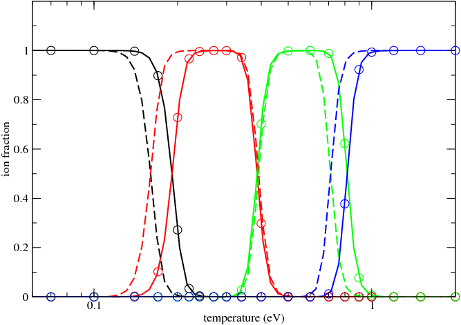
Figure 2: Ionization-stage fraction versus temperature for Nd at a typical mass density of $\rho=10^{-13}$ g/cm³, calculated with the fully relativistic (FR) approach. The black curves and circles refer to Nd i, the red ones to Nd ii, the green ones to Nd iii, and the blue ones to Nd iv. The solid curves use NIST-corrected ionization energies (Kramida et al., 2018), while the dashed curves use uncorrected values. The circles indicate explicit temperatures at which (NIST-corrected) opacities were calculated for use in the simulation of spectra and light curves.

Due to the relatively low densities associated with the dynamical ejecta, a single ion stage is dominant over a broad range of temperatures. This behavior is typical for all of the elements considered in this work because the ionization energy of each of their first three ion stages is similar (see, for example, Table 1).

2.3 Variant Models

In addition to calculating FR and SR models, two less-accurate (but faster to compute) FR models were generated in order to test the sensitivity of the kilonova emission to the quality of the atomic data. Configuration interaction (CI) is a method to better describe the correlation between the bound electrons of an atom or ion, and typically results in improved level energies and oscillator strengths (for a more detailed explanation, see, for example, Cowan 1981; Fontes et al. 2015b). The use of CI is crucial for obtaining reasonably accurate atomic structure data for the near-neutral heavy elements considered here. However, due to the smearing of lines caused by the large velocity gradients in the ejecta, it is possible that differing amounts of CI could produce similar spectra, which, if true, would provide more confidence in the fidelity of the simulated spectra, at least from an atomic physics perspective.

In order to test this concept, we generated two additional FR models for Nd: one that includes CI between only those basis states that arise from the same relativistic configuration and one that includes CI between only those basis states that arise from the same non-relativistic configuration. These models are referred to here as “FR-SCR” and “FR-SCNR”, respectively (see Fontes et al. 2015b, 2016 for additional details). The FR-SCR model is less accurate than the FR-SCNR model, which is less accurate than the FR model described above. All three FR models contain the same number of fine-structure levels, but their energies differ due to the different CI treatments. Additionally, each model contains a different number of lines, as displayed in Table 2. The variant models have fewer lines than the baseline FR model, and those transitions that are common to the three models will typically be described by different oscillator strengths.

Table 2: Number of lines per ion stage of neodymium for the FR, FR-SCNR and FR-SCR models (see text).

Ion stage	# of lines
	FR	FR-SCNR	FR-SCR
Nd i	25,224,451	14,330,369	2,804,438
Nd ii	3,958,977	3,222,445	783,275
Nd iii	233,822	137,192	51,036
Nd iv	5,784	5,393	2,051

3 Sample Opacities and Tables

In order to illustrate the basic characteristics of the opacities used in this study, the LTE monochromatic opacity for Nd is displayed in Figure 3 for typical ejecta conditions of $T=0.5$ eV and $\rho=10^{-13}$ g/cm³.

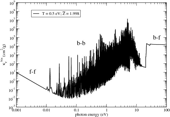
Figure 3: The LTE line-binned opacity for neodymium at $T=0.5$ eV and $\rho=10^{-13}$ g/cm³. The left panel displays the complete opacity, which includes the bound-bound, bound-free, free-free and scattering contributions. The right panel displays only the contributions due to free electrons, i.e. the free-free and scattering contributions. The average charge state, $\overline{Z}$, for these conditions is listed in the legend of the left panel.

The left panel displays the complete opacity, with all four contributions (b-b, b-f, f-f and scattering), while the right panel shows the contributions that arise only from free electrons (f-f and scattering) in order to give some indication of the massive differences that occur when the bound electrons are taken into account. The b-b contribution was calculated via the line-binned expression in Equation (2). The f-f and scattering contributions were obtained from the simple, analytic formulas (Huebner & Barfield, 2014) associated with Thomson and Kramers, respectively. The gap between the b-b features and the onset of the b-f edge occurring at $\sim 20$ eV is due to missing lines that would be present if more excited configurations had been included in the model. Our transport calculations have minimal intensity at these energies. We note that a mean charge state of $\overline{Z}=1.998$ is obtained for these conditions, indicating that the opacity is dominated by Nd iii.

In this example, the inclusion of the line features dramatically increases the opacity in the optical range (1.65–3.26 eV or 0.751–0.380 $\mu$m) by up to eight orders of magnitude. The absorption in the near-infrared range below 1.65 eV (0.496–1.65 eV or 10.0–0.751 $\mu$m) is also greatly increased, by a few orders of magnitude in this case, indicating that spectra would more likely be observed in the mid-infrared range, at least for these specific conditions.

3.1 Examples of line-binned opacities

A more detailed Nd opacity example is provided in Figure 4, with the conditions ($T=0.5$ eV, $\rho=10^{-13}$ g/cm³) being the same as those given in Figure 3.

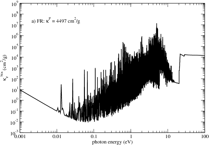
Figure 4: The LTE line-binned opacity for neodymium at $T=0.5$ eV and $\rho=10^{-13}$ g/cm³ using four different models described in the text: a) FR, b) FR-SCNR, c) FR-SCR, and d) SR. The Planck mean opacity, obtained via integration of the line-binned opacity, is also listed in each panel.

Line-binned opacities are presented for the four models described in Section 2: FR, FR-SCNR, FR-SCR, SR. The models produce qualitatively similar results, but there are visible quantitative differences, as exemplified by the Planck mean opacities displayed in each panel. The Planck mean opacity is defined in the standard way, i.e.

$$\kappa^{\rm P}\equiv\int_{0}^{\infty}B_{\nu}(T)\kappa_{\nu}^{\prime}\,d\nu\Big{/}\int_{0}^{\infty}B_{\nu}(T)\,d\nu\,,$$ (4)

where $B_{\nu}(T)$ is the Planck function and $\kappa_{\nu}^{\prime}$ indicates that the scattering contribution is omitted from the monochromatic opacity. This mean value of the frequency-dependent opacity permits rough quantitative comparisons between models. The SR model produces the smallest mean value, given by 3727 cm²/g, while the least accurate FR-SCR model has a value of 5299 cm²/g, resulting in a variation of 42%. The most accurate FR model produces an intermediate value of 4497 cm²/g, with the FR-SCNR yielding a similar result. These differences allow us to test the sensitivity of the kilonova light curves and spectra (see Section 4) to changes in the underlying atomic physics models that are used to construct the opacity.

Next, we consider a broader range of elements at a cooler temperature, presenting line-binned opacities for the four representative elements (Ce, Nd, Sm and U) at $T=0.3$ eV, $\rho=10^{-13}$ g/cm³ in Figure 5.

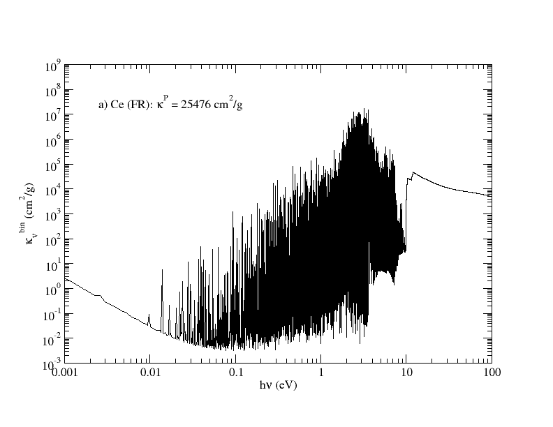
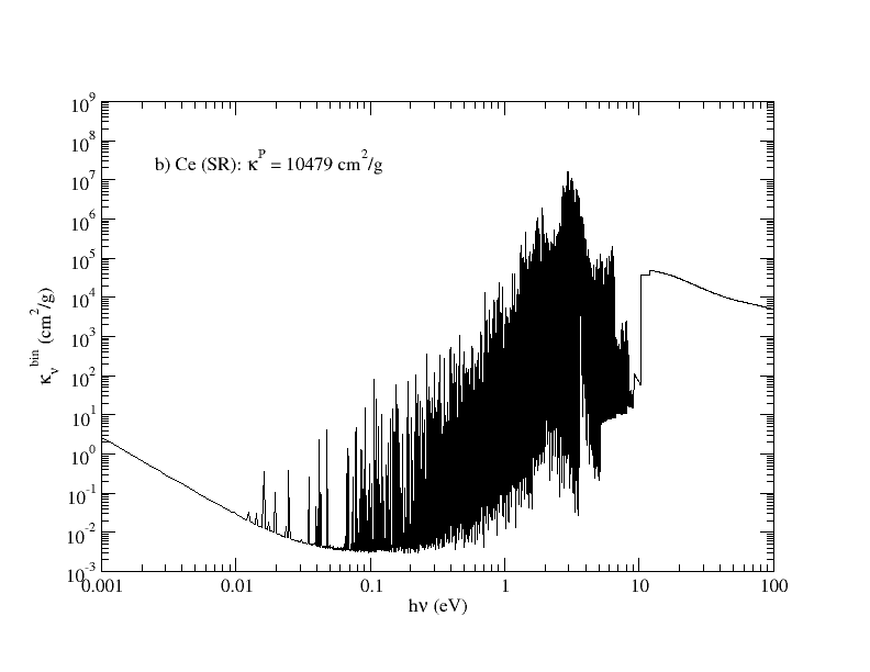
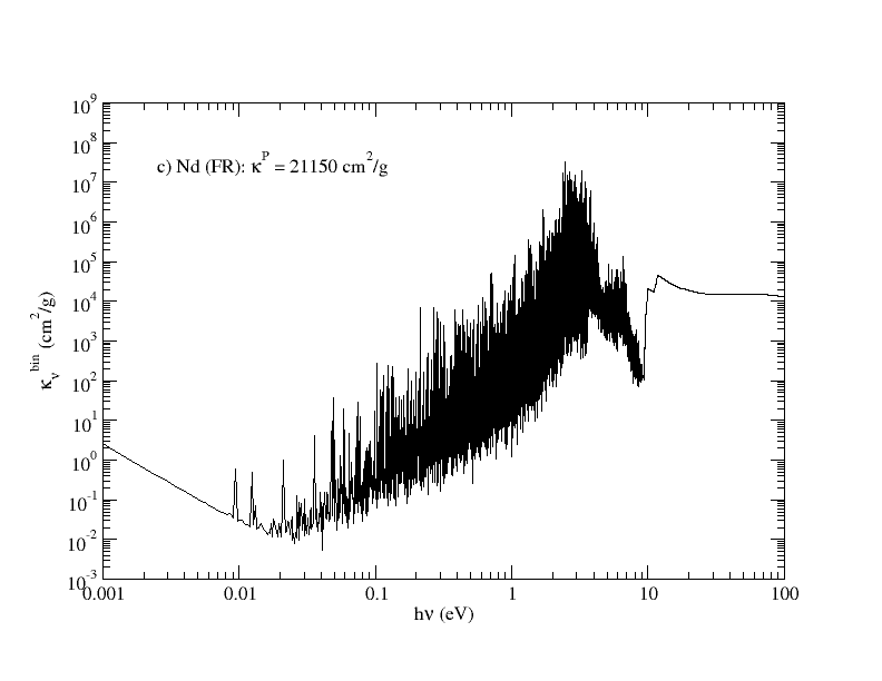
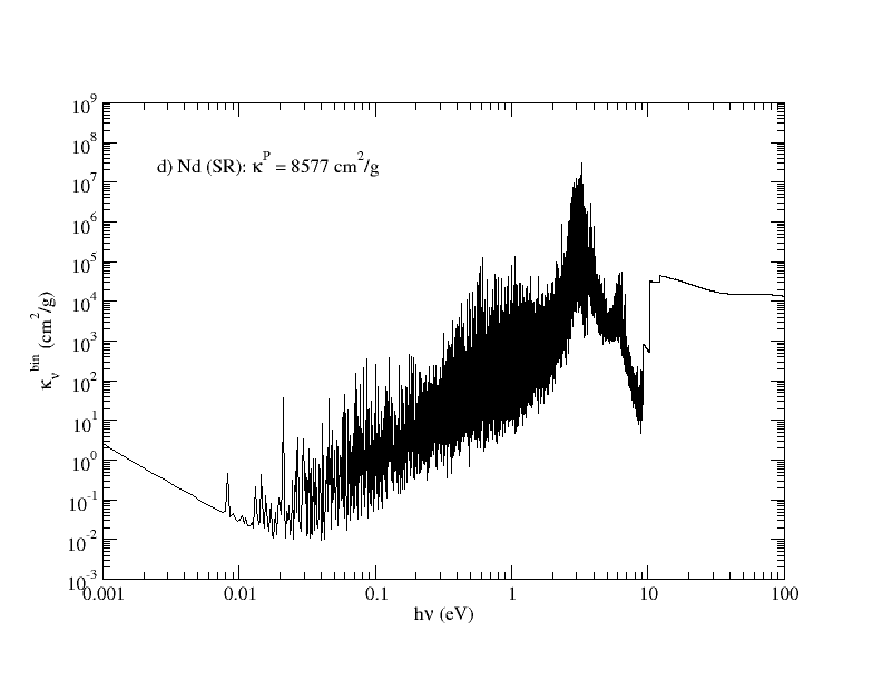
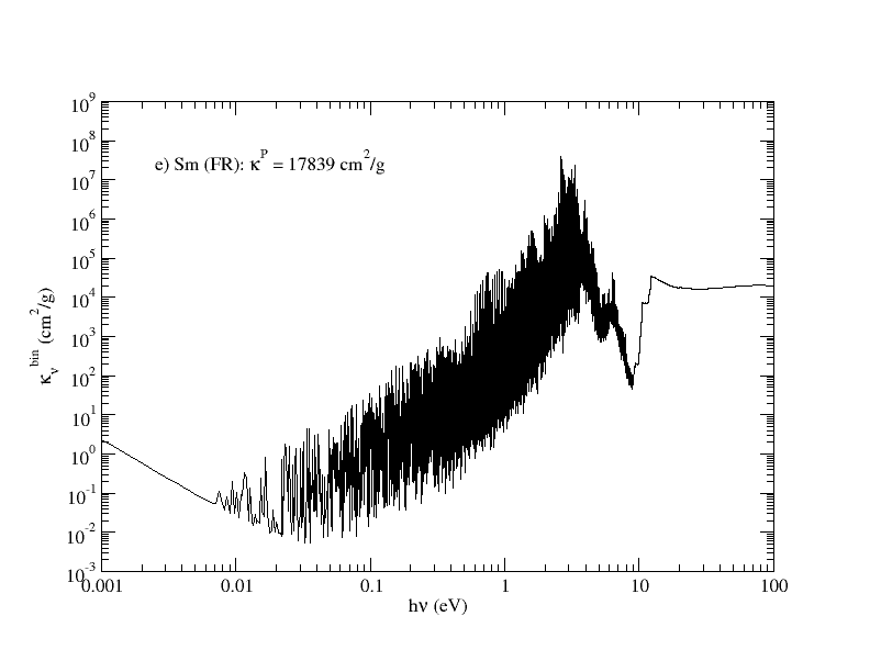
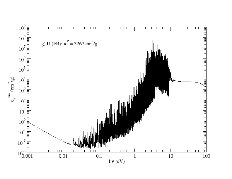
Figure 5: LTE line-binned opacities for four representative elements (Ce, Nd, Sm and U) at $T=0.3$ eV and $\rho=10^{-13}$ g/cm³. Panels a & b represent Ce, panels c & d represent Nd, panels e & f represent Sm, and panels g & h represent U. The panels in the left column were calculated with the FR approach, while panels in the right column were calculated with the SR approach. The Planck mean opacity, obtained via integration of the line-binned opacity, is also listed in each panel.

Results are displayed for both FR and SR results in order to compare these two different atomic physics models for a range of elements. The opacities for all of these elements display similar qualitative behaviors: line-dominated absorption that increases with photon energy, with a peak at $\sim 3$ eV, and a bound-free edge at an energy of $\sim 10$ eV. These similarities are not surprising because the charge state distribution for each element is dominated by the second ion stage, i.e. $\overline{Z}\approx 1$, at these conditions. Therefore, the bound-bound contribution to the opacity is dominated by lines associated with the singly ionized stage for each element in this example. As explained in Section 2.2, and demonstrated in Figure 2 and Table 1, a single ion stage is dominant over a broad range of temperature at such low densities for a given element. Furthermore, the dominant stage is typically the same for all lanthanide (and actinide) elements due to the similarity in the ionization potentials of their ion stages.

Despite these comparable trends, an inspection of the frequency-dependent opacities also reveals the differences inherent in the underlying atomic energy-level structure for each element. The detailed line structure is visibly different in each panel of Figure 5 due to fundamental atomic physics theory concepts such as the angular momentum coupling between the various bound electrons, quantum selection rules for the absorption of photons between different energy levels, etc. There are also notable differences when comparing the FR and SR values for a given element. The Planck mean opacity is, once again, presented in each panel of Figure 5 for comparison purposes. The ratio of the FR to SR value of the Planck mean is 2.43, 2.47, 1.74 and 0.889 for Ce, Nd, Sm and U, respectively. The variation in this set of ratios gives a basic indication of the uncertainty in the opacities due to the choice of physics models for this group of four elements. Within the FR or SR model, the maximum ratio occurs between Ce and U, with a value of 7.80 or 2.85, respectively. These two values provide a rough estimate of how the opacity can vary between different elements calculated within the same physical framework. Of course, representing such complex, frequency-dependent absorption features by a single mean value is a gross approximation. A more realistic comparison should investigate the use of different opacity models in the simulation of kilonova emission, which we consider in Section 4.

As a final illustration, we present in Figures 6 and 7 the line-binned opacity for all 14 lanthanide elements, as well as uranium, at two sets of characteristic conditions. These results were calculated with the SR model.

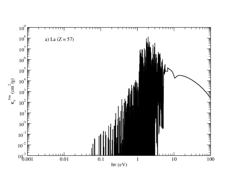
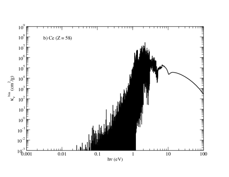
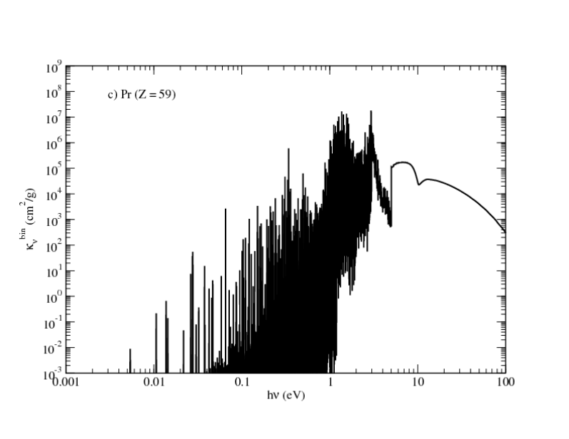
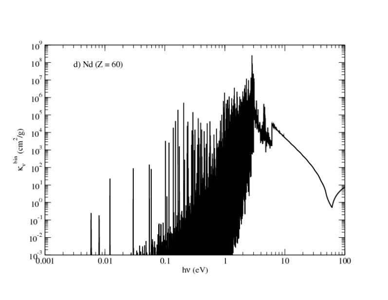
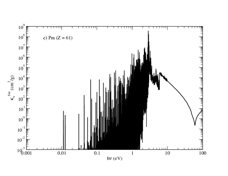
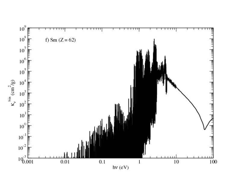
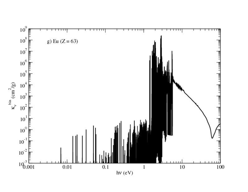
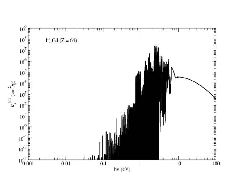
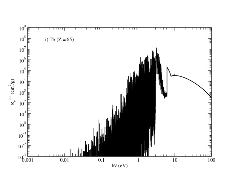
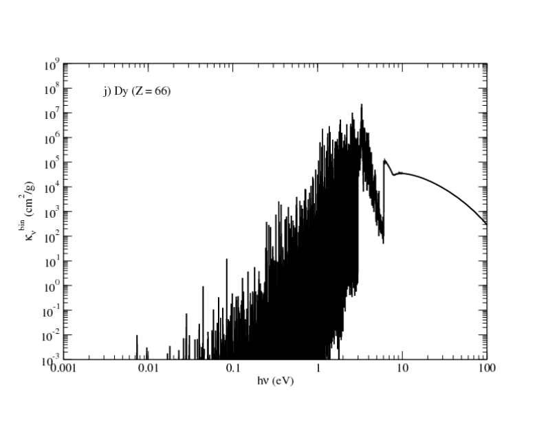
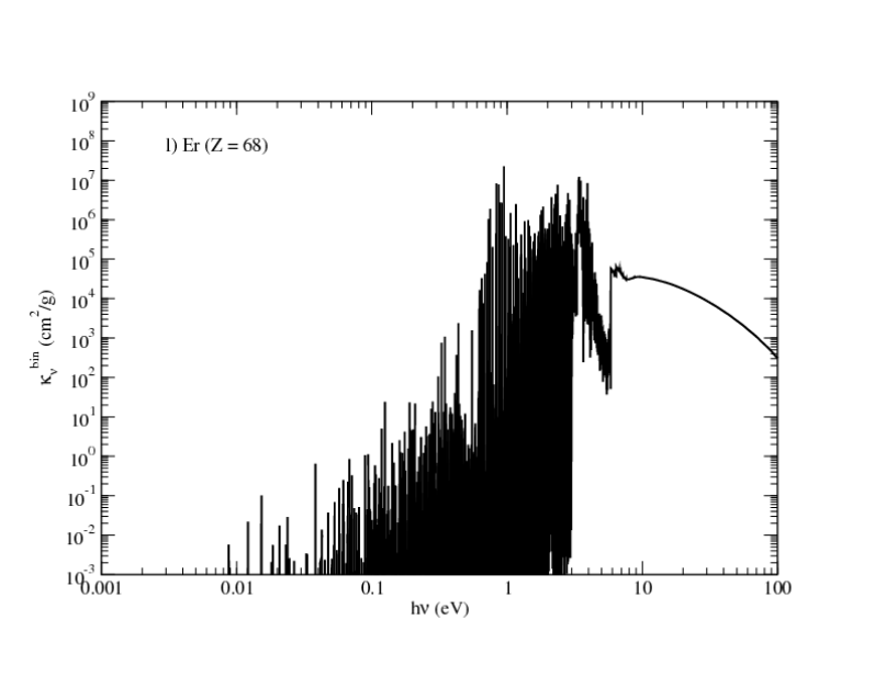
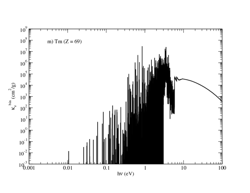
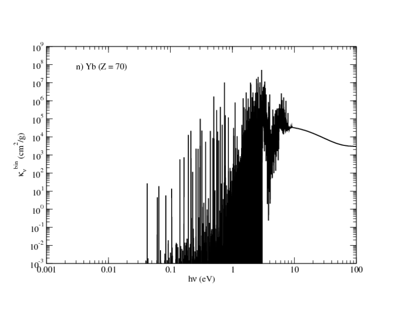
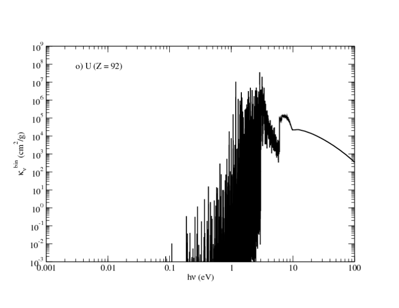
Figure 6: The LTE line-binned opacity for all 14 lanthanide elements, as well as uranium, at $T=0.1$ eV and $\rho=10^{-13}$ g/cm³. For these conditions, the bound-bound contribution to the opacity is dominated by the first, i.e. neutral, ion stage of each element. Panels a–n display results for $Z=$57–70, while panel o displays the uranium ($Z=92$) result.

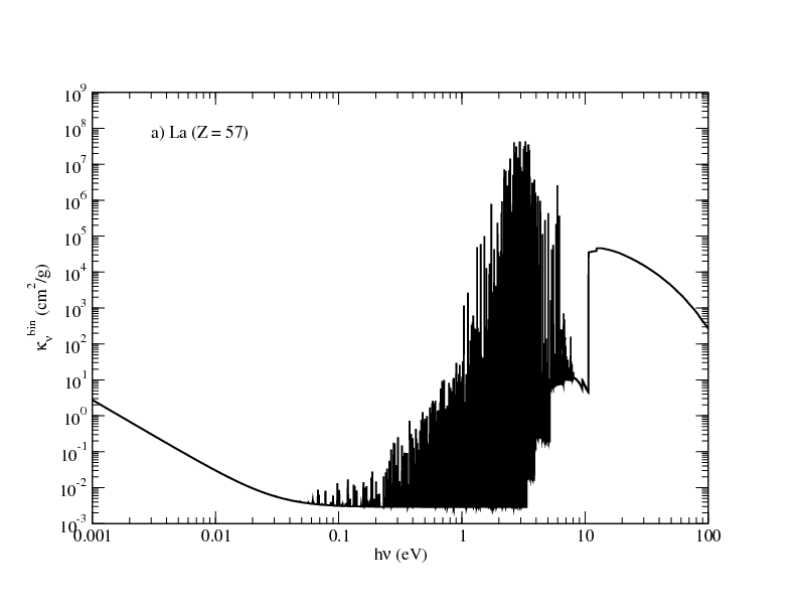
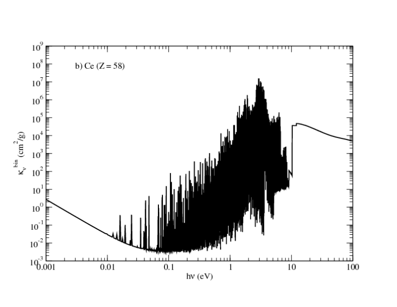
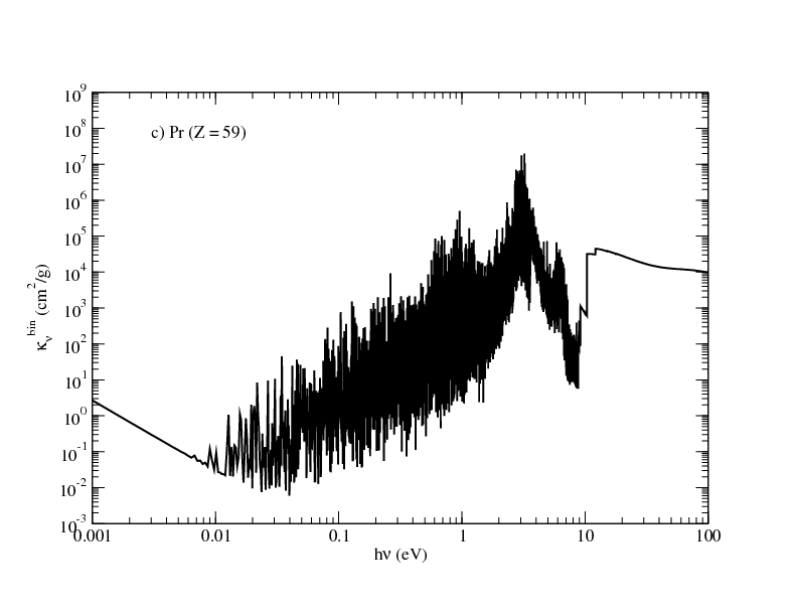
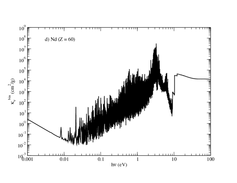
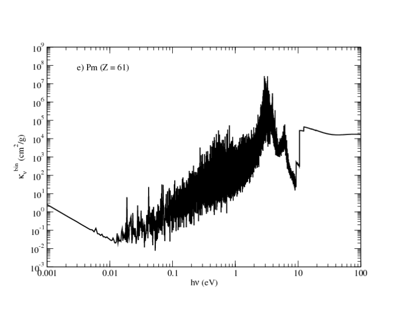
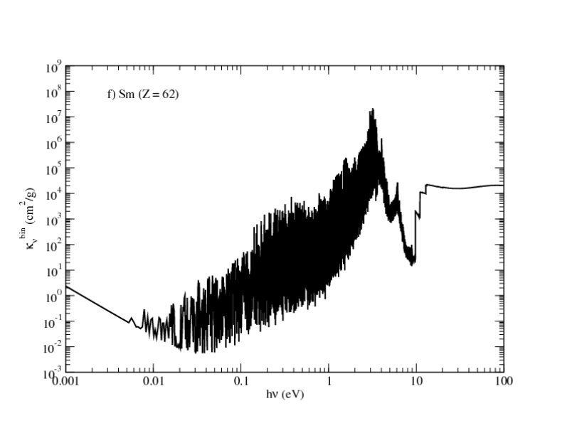
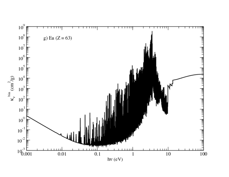
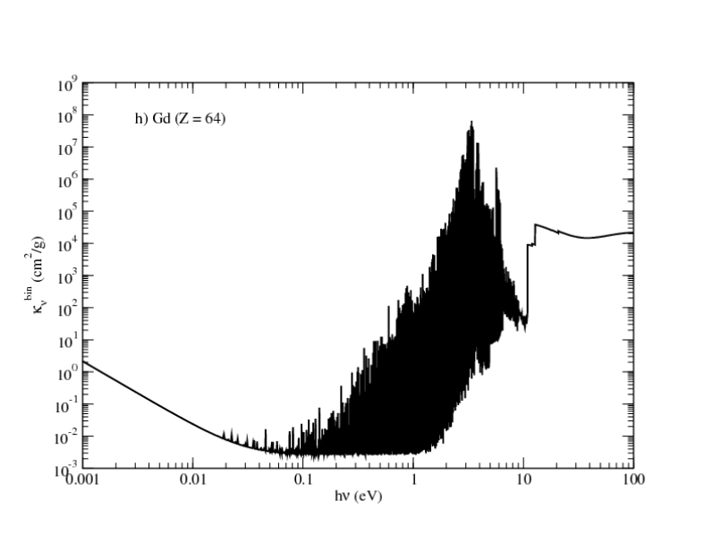
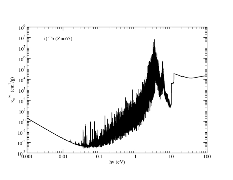
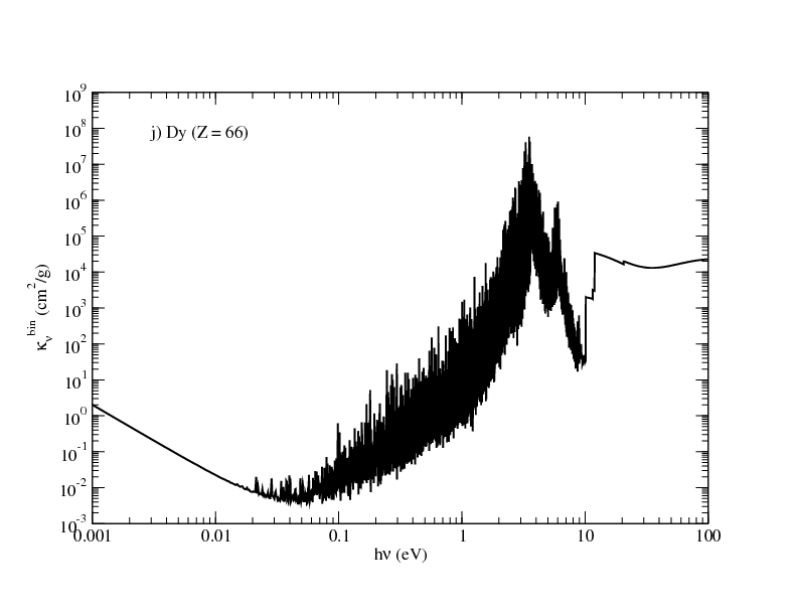
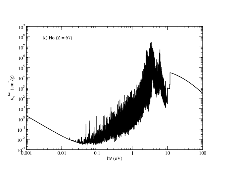
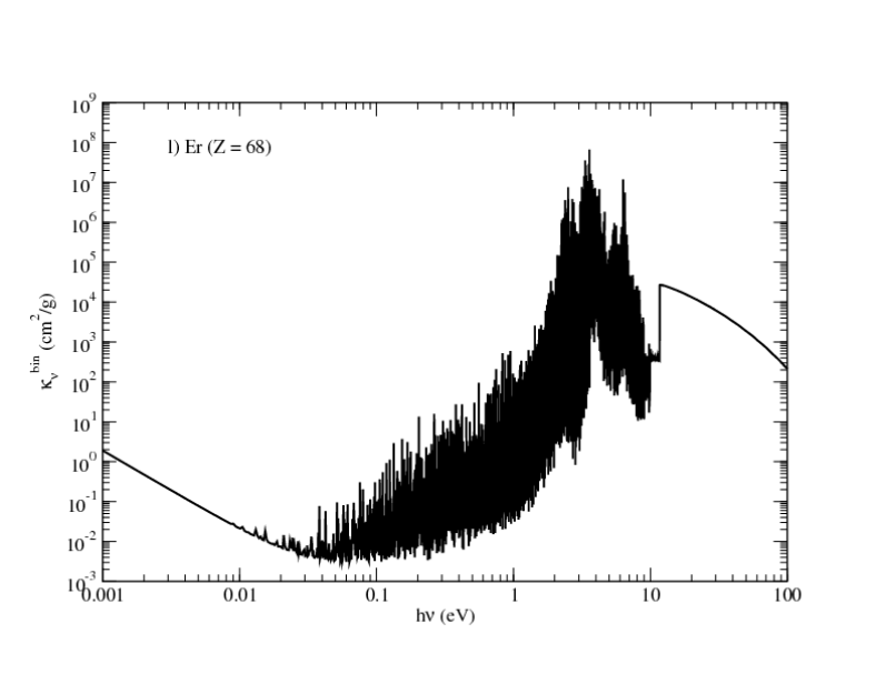
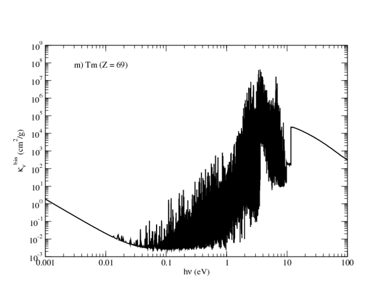
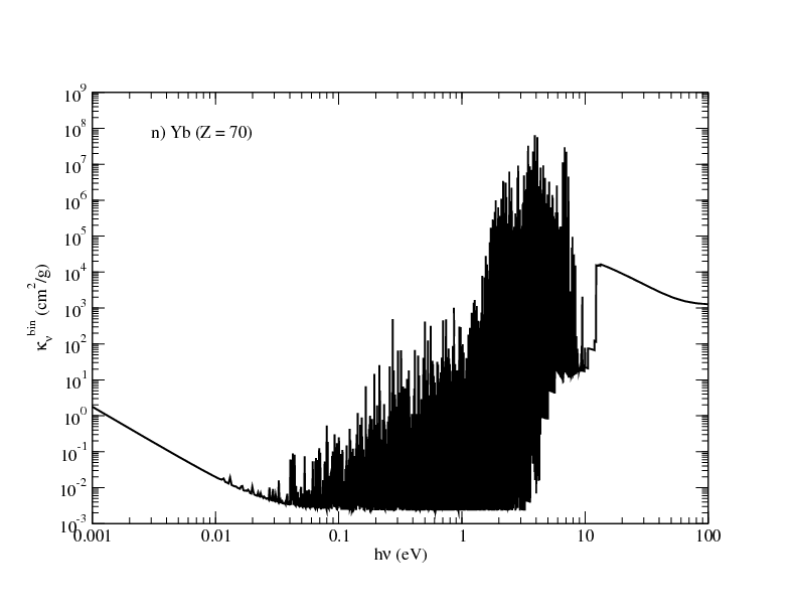
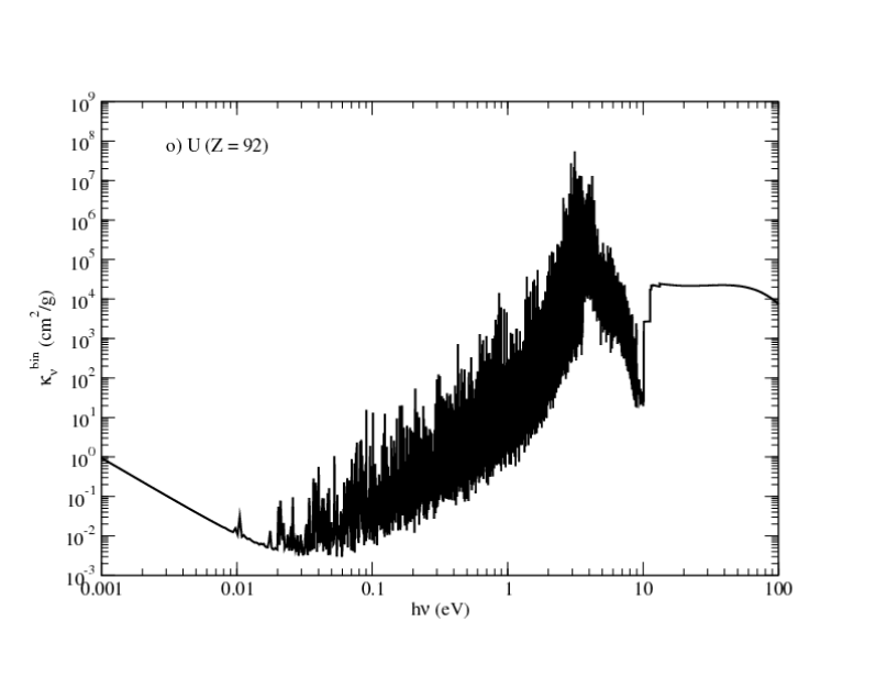
Figure 7: The LTE line-binned opacity for all 14 lanthanide elements, as well as uranium, at $T=0.3$ eV and $\rho=10^{-13}$ g/cm³. For these conditions, the bound-bound contribution to the opacity is dominated by the second, i.e. singly ionized, ion stage of each element. Panels a–n display results for $Z=$57–70, while panel o displays the uranium ($Z=92$) result.

Once again, a characteristic ejecta density of $\rho=10^{-13}$ g/cm³ was chosen for both figures. A temperature of $T=0.1$ eV was chosen in Figure 6 to highlight opacities with a b-b contribution that is dominated by the first, i.e. neutral, ion stage for all 15 elements. A higher temperature of $T=0.3$ eV was chosen in Figure 7 to compare opacities with a b-b contribution that is dominated by the second, i.e. singly ionized, ion stage of each element.

The qualitative trends in these two figures resemble those discussed above for Figures 4 and 5. For example, the opacity for all 15 elements in Figures 6 and 7 displays line-dominated absorption that increases with photon energy, peaking at an energy of about 2–3 eV. In Figure 6, the signature f-f and scattering contributions (see Figure 3) are absent because the underlying atomic proceseses of inverse bremsstrahlung and electron scattering, respectively, require the presence of free electrons. Since the charge state distribuion is dominated by the neutral ion stage in this case, $\overline{Z}\approx 0$ and the free electron density is relatively small. On the other hand, the f-f and scattering contributions are clearly present in Figure 7 for which the temperature, and free electron density, is higher.

In order to provide some qualitative analysis of the line-binned opacities for the 14 lanthanide elements displayed in Figures 6 and 7, we present Figures 8 and 9, respectively.

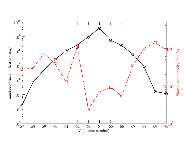
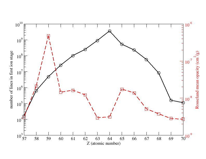
Figure 8: The number of lines in the first ion stage versus atomic number, $Z$ (see Table 4). The mean opacity associated with the line-binned opacities presented in Figure 6 is also plotted versus $Z$. Results are presented for all 14 lanthanide elements ($Z=57$–70). In both panels, the number of lines for the first ion stage is represented by the black solid curve (with circles). This curve is associated with the left-hand $y$ axis in each panel. The red dashed curves (with squares) are assocated with the right-hand $y$ axis in each panel, and represent the Planck mean opacity in the left panel and the Rosseland mean opacity in the right panel. The mean opacities were calculated at $T=0.1$ eV and $\rho=10^{-13}$ g/cm³, corresponding to the conditions used in Figure 6.

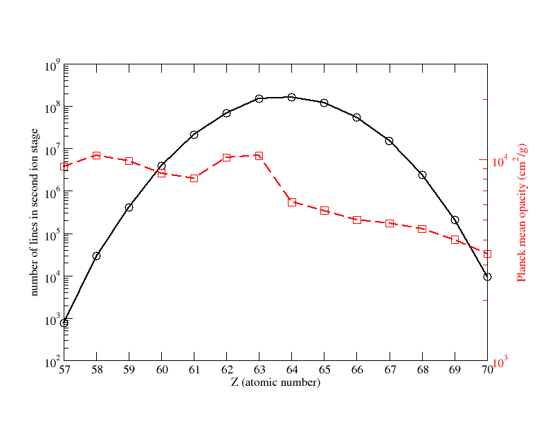
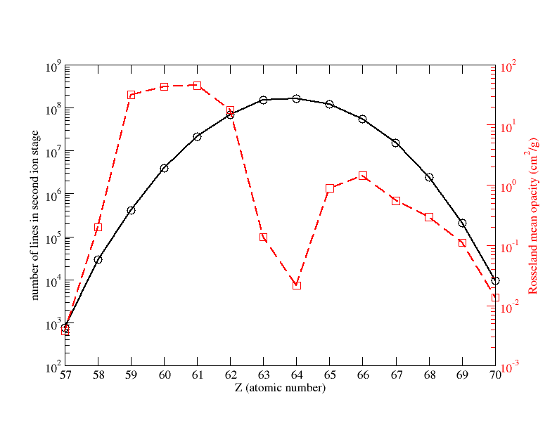
Figure 9: The number of lines in the second ion stage versus atomic number, $Z$ (see Table 4). The mean opacity associated with the line-binned opacities presented in Figure 7 is also plotted versus $Z$. Results are presented for all 14 lanthanide elements ($Z=57$–70). In both panels, the number of lines for the second ion stage is represented by the black solid curve (with circles). This curve is associated with the left-hand $y$ axis in each panel. The red dashed curves (with squares), assocated with the right-hand $y$ axis in each panel, represent the Planck mean opacity in the left panel and the Rosseland mean opacity in the right panel. The mean opacities were calculated at $T=0.3$ eV and $\rho=10^{-13}$ g/cm³, corresponding to the conditions used in Figure 7.

In each of the two panels in Figure 8, the solid black curve (with circles) represents the number of lines in the first ion stage, which is the dominant stage for these conditions, for each element. The number of lines for the various ion stages can also be found in Table 4. Superimposed on this black curve is a red dashed curve (with squares) that represents the mean opacity obtained from the frequency-dependent opacities in Figure 6. The red dashed curve in the left panel represents the Planck mean opacity displayed in Equation (4). The red dashed curve in the right panel represents the Rosseland mean opacity defined by the standard harmonically averaged expression

$$[\kappa^{\rm R}]^{-1}\equiv\int_{0}^{\infty}B_{\nu}^{\prime}(T)[\kappa_{\nu}]^{-1}\,d\nu\Big{/}\int_{0}^{\infty}B_{\nu}^{\prime}(T)\,d\nu\,,$$ (5)

where $B_{\nu}^{\prime}(T)$ is the partial derivative of the Planck function with respect to temperature.

As expected from basic atomic physics considerations, the number of lines in the first ion stage of the 14 lanthanide elements peaks at Gd $(Z=64)$, near the center of the range. The energy level structure of Gd is the most complicated due to the presence of the half-filled $4f^{7}$ subshell, as well as a $5d^{1}$ subshell, in the ground-state configuration. This combination of open subshells results in a maximum in the number of fine-structure levels that are allowed by quantum physics, i.e. according to the rules of angular momentum coupling of the bound electrons and the Pauli exclusion principle. This large number of levels corresponds to a maximum in the number of lines (or transitions) displayed in Figure 8. However, this peak in the number of lines corresponds to relatively low values in the Planck and Rosseland mean opacities. This is a counterintuitive result since the existence of more lines is expected to increase the chances of photon absorption, which corresponds to higher opacities. In addition, note that the adjacent element Eu $(Z=63)$, which also contains the $4f^{7}$ subshell in its ground configuration, similarly corresponds to relatively low values of the two mean opacities. This behavior can be understood from the fact that the half-filled $4f^{7}$ subshell is semi-stable with respect to energy, i.e. it takes more energy to excite an electron from this type of configuration than it does from the adjacent ground configurations that contain the $4f^{6}$ or $4f^{8}$ subshell. Thus, the energy-level structure associated with an element possessing a $4f^{7}$ subshell in its ground state can be somewhat different than the other lanthanides, and a significant fraction of the allowed radiative transitions can occur at higher energies than for the other lanthandides. For example, according to the NIST database (Kramida et al., 2018), the first excited state of Eu i occurs at an energy of $\sim 1.6$ eV. This value is a factor 2–60 higher than the first excited state in the neutral stage of most of the other lanthanides, indicating that the energy-level structure of Eu i is different. Consequently, the number of lines appearing in the Eu (panel g) and Gd (panel h) opacities displayed in Figure 6 is indeed higher than the number for the other elements, but a significant fraction of those lines occurs at relatively higher energies, above $\sim 1$ eV in this case. Since the Planck and Rosseland weighting functions peak at photon energies of $\sim 2.8\times T$ and $\sim 3.8\times T$, respectively, those higher energy lines do not contribute as much to the mean opacities. Similar trends are observed in Figure 7 for which the second ion stage is dominant. The maximum number of lines occurs for Gd, but the Rosseland mean value, represented by the red dashed curve in the right panel, is at a minimum. The Planck mean does not display such a definitive minimum value, but there is a significant drop at Gd when traversing the red dashed curve displayed in the left panel from lower to higher values of $Z$.

The above trends suggest that, counter to conventional wisdom, the elements in the middle of the lanthanide range might not produce the strongest contributions to the opacity of dynamical ejecta in kilonovae. We emphasize that the use of Planck and Rosseland mean values in the above analysis is for illustrative purposes and should be interpreted with a measure of caution. A study of the relative importance of the various lanthanide elements to the ejecta opacity could be investigated with kilonova simulations that employ the frequency-dependent opacities, which is beyond the scope of this work.

3.2 Line-smeared opacities

In previous work (Fontes et al., 2015a, 2017), we presented a preliminary attempt to generate tabular opacities that also preserved the integral of the monochromatic opacities over frequency. This effort employed a line-smeared approach to artificially broaden the lines in such a manner that they could be sufficiently resolved with a typical photon energy grid (see Section 3.4) employed in a tabular framework. These line-smeared opacities were also used in a detailed study of NSM light curves and spectra (Wollaeger et al., 2018). Thus, some commentary about how the line-smeared and line-binned opacities compare is provided here.

The present line-binned approach accomplishes the desired goal of preserving the area under the opacity curve without the concern of losing b-b opacity due to a lack of photon energy resolution. The use of a discrete sum in the line-binned approach, see Equation (2), ensures that the area will be conserved and, furthermore, allows fine-structure detail to be more easily captured in a tabular representation of the opacities. As a specific example, we present a comparison of the LTE Nd multigroup opacity, $\kappa^{\rm group}_{\lambda,{\rm g}}$, generated with the line-binned and line-smeared methods in Figure 10 for the characteristic conditions of $T=0.3$ eV and $\rho=10^{-13}$ g/cm³. The multigroup opacities were generated using the wavelength version of the frequency-group opacity displayed in Equation (3), with a group structure of 1,024 logarithmically spaced wavelength points (see Section 4.2 for details). As expected, the overall agreement between the two curves is good, but the line-binned curve clearly displays more fine-structure detail at higher wavelengths. This additional detail in the line-binned curve is a result of summing the unbroadened lines within a wavelength bin, rather than smearing the lines across a number of bins, in conjunction with the fact that the resolution of the groups are on par with the resolution of the bins at higher wavelengths. Despite these differences, the line-binned and line-smeared opacities yield similar kilonova spectra (see Section 4.2.2 and, specifically, Figure 14).

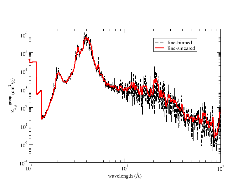
Figure 10: The LTE multigroup opacity of Nd at $T=0.3$ eV and $\rho=10^{-13}$ g/cm³. Results are presented for the line-binned (dashed black curve) and line-smeared (solid red curve) methods using 1,024 wavelength groups (see text for details).

3.3 Expansion opacities

In order to provide meaningful comparisons with other works, we also consider the more traditional approach of expansion opacities when modeling light curves and spectra in Section 4. Therefore, a brief overview of this approach is provided here. As mentioned previously, the expansion-opacity method (Sobolev, 1960; Castor, 1974; Karp et al., 1977) employed by Kasen et al. (2013); Barnes & Kasen (2013) to simulate kilonovae light curves applies to the bound-bound contribution to the opacity and involves a discrete sum over all lines. The approach relies on the assumption of a homologous expansion and is characterized by an expansion time, $t_{\rm exp}$. The relevant wavelength range is divided into bins denoted by index $j$, $\Delta\lambda_{j}$, and all lines within a bin are summed to obtain the opacity for that range. The expression for the opacity associated with bin (or group) $j$ is given by

$$\kappa^{\rm b-b}_{\rm exp}(\Delta\lambda_{j})=\frac{1}{\rho ct_{\rm exp}}\sum_{i\in\Delta\lambda_{j}}\frac{\lambda_{i}}{\Delta\lambda_{j}}(1-e^{-\tau_{i}})\,,$$ (6)

where $t_{\rm exp}$ is the time since mass ejection, the summation index $i$ extends over all bound-bound transitions that reside in bin $j$, $\lambda_{i}$ is the rest wavelength associated with transition $i$, and $\tau_{i}$ is the corresponding Sobolev optical depth, i.e.

$$\tau_{i}=\frac{\pi e^{2}}{m_{e}c}\,N_{i}\,|f_{i}|\,t_{\rm exp}\,\lambda_{i}\,,$$ (7)

which is the Doppler-corrected line optical depth. Due to the presence of $t_{\rm exp}$ in the exponential of Equation (6), it is not convenient to construct tables of the expansion opacities for kilonova modeling.

As a specific example, we present in Figure 11 the expansion opacity of Nd at $T=$ 4,000 K ($0.345$ eV) and $\rho=10^{-13}$ g/cm³, generated with the FR model.

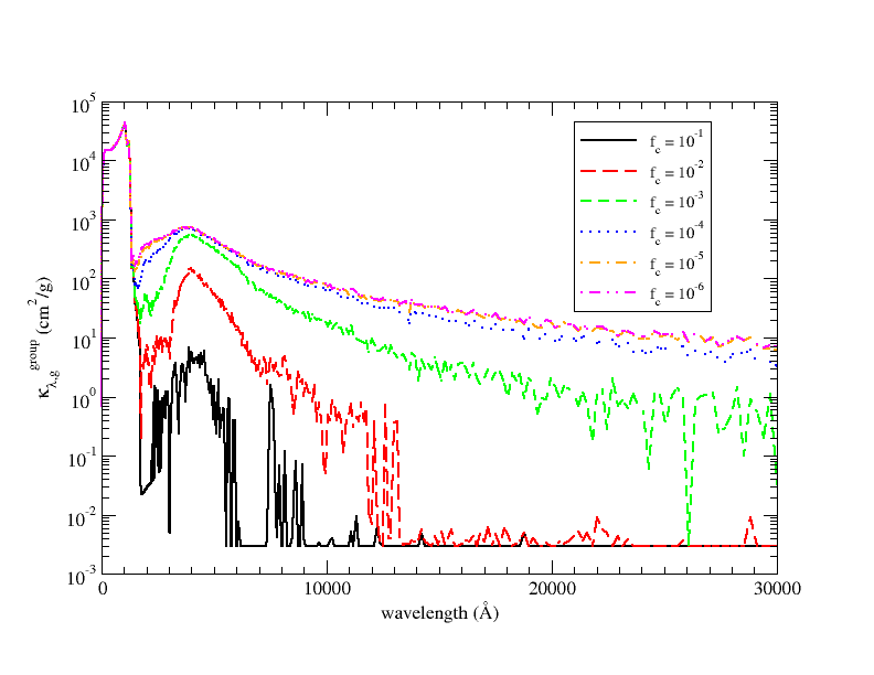
Figure 11: The LTE opacity of Nd at $T=4,000$ K ($0.345$ eV) and $\rho=10^{-13}$ g/cm³ using the expansion-opacity method. The time since ejection was chosen to be $t_{\rm exp}=1$ day, along with a wavelength group structure of $\Delta\lambda=0.01\lambda$. These specifications are the same as those considered in Figure 8 of Kasen et al. (2013). The various curves correspond to different values of the oscillator strength cutoff paramater, $f_{c}$, as follows: solid (black) curve represents $10^{-1}$, long-dashed (red) curve represents $10^{-2}$, short-dashed (green) curve represents $10^{-3}$, dotted (blue) curve represents $10^{-4}$, dash-dotted (orange) curve represents $10^{-5}$, and dash-double-dotted (magenta) curve represents $10^{-6}$. Convergence is obtained for a value of $f_{c}=10^{-6}$.

In this example, the opacity is plotted versus wavelength instead of energy, and the particular conditions were chosen in order to facilitate a direct comparison with Figure 8 of Kasen et al. (2013).

There are six curves displayed in Figure 11, corresponding to different values of the oscillator strength cutoff, $f_{c}=10^{-x}$, with $x=$ 1–6. Convergence is demonstrated for $f_{c}=10^{-6}$, which is the same value that we chose when constructing our tabular, line-binned opacities. (See Section 2.1.) The use of such tabular opacities is particularly convenient when exploring opacity models constructed with different line strength cutoff values. A sensitivity study of light-curve and spectral modeling to the value of $f_{c}$ is presented in Section 4.

A comparison of Figure 11 with Figure 8 of Kasen et al. (2013) allows a relatively direct comparison of the underlying opacity data employed in each investigation, in contrast to comparisons of spectral quantities resulting from radiation transport simulations that sample the opacity over a range of physical conditions. We note that the upper four curves in Figure 11 are qualitatively similar to the curves displayed in Figure 8 of Kasen et al. (2013), with the peak value of the b-b contribution occurring at $\sim$5,000 Å and monotonically decreasing at higher wavelengths. However, the peak value is about three times larger in the present case, providing a rough measure of the uncertainty in current opacity calculations as they pertain to kilonova conditions.

This discrepancy is somewhat surprising due to the fact that the same list of configurations, resulting in the same number of lines (see the Nd data listed in Table 4), was used in both cases. The differences are perhaps an indication of how difficult it is to perform accurate atomic structure calculations for such complicated atoms and ions. An alternative explanation is that the curves displayed in Figure 8 of Kasen et al. (2013) were generated with a less complete set of lines. This potential explanation is supported by the observation that the short-dashed (green) curve in Figure 11, which was generated with a value of $f_{c}=10^{-3}$, is in better agreement with Kasen et al. (2013) over the entire wavelength range. This improved agreement includes the large oscillatory behavior at high wavelengths, although our green curve is still a factor of two higher at the peak value occurring at $\sim$5,000 Å. Another qualitative difference occurs at higher wavelengths, where there appear to be more points in the curves of Kasen et al. (2013). We were able to obtain similar behavior (not shown) in the high-wavelength region by employing a linearly spaced wavelength grid, rather than the logarithmically spaced grid obtained from the prescription $\Delta\lambda=0.01\lambda$.

As a final opacity comparison, we present in Figure 12 the line-binned and expansion opacities of Nd at the same conditions used for Figure 11.

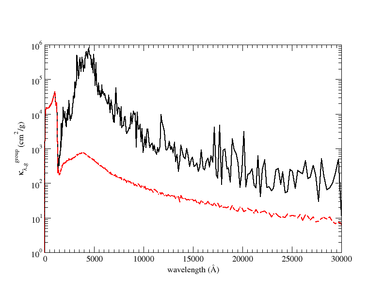
Figure 12: The LTE opacity of Nd at $T=4,000$ K ($0.345$ eV) and $\rho=10^{-13}$ g/cm³ using the line-binned (solid, black curve) and expansion-opacity (dashed, red curve) methods to obtain the b-b contribution. For the expansion-opacity calculation, the time since ejection was chosen to be $t_{\rm exp}=1$ day. In both cases, a wavelength group structure of $\Delta\lambda=0.01\lambda$ was chosen. These specifications are the same as those considered in Figure 8 of Kasen et al. (2013) and Figure 7 of Fontes et al. (2017).

There are two curves in the figure, one representing the bound-bound contribution obtained from the current line-binned approach, Equation (2), and the other from the expansion-opacity method, Equation (6). Both curves were generated with the FR model. (For completeness, we mention that the two corresponding curves generated with the SR model (not shown) are quantitatively similar to the two FR curves displayed in this figure.) We note that, for these conditions, the line-binned approach produces an opacity that is one or more orders of magnitude greater than the expansion method over much of the wavelength range. As expected, these trends are very similar to the behavior exhibited in the corresponding comparison of line-smeared versus expansion opacities in Figure 7 of Fontes et al. (2017). In general, the area-preserving opacities are expected to be equal to or greater than the expansion opacities based on a simple examination of the mathematical behavior of Equations (6) and (7) versus Equation (2). (Compare, also, Equation (8) to Equation (9) in the upcoming Section 4.1.) As a consequence, the luminosity is expected to be diminished when line-binned opacities, rather than expansion values, are used when simulating light curves. However, the deviation in the resulting light curves depends on a broad range of conditions that are relevant for a complete simulation, and can not be determined from a simple opacity comparison carried out at a specific set of conditions.

3.4 Opacity tables

In order to perform radiation-transport calculations in an efficient manner, opacity tables were generated for the 15 elements discussed above using prescribed temperature and density grids that span the range of conditions of interest. The temperature grid consists of 27 values (in eV): 0.01, 0.07, 0.1, 0.14, 0.17, 0.2, 0.22, 0.24, 0.27, 0.3, 0.34, 0.4, 0.5, 0.6, 0.7, 0.8, 0.9, 1.0, 1.2, 1.5, 2.0, 2.5, 3.0, 3.5, 4.0, 4.5, and 5.0. Specific temperature values are also indicated by circles in the ionization balance plot of Figure 2. The density grid contains 17 values ranging from 10^-20 to 10^-4 g/cm³, with one value per decade. Our photon energy grid is the same 14,900-point grid that is used in standard Los Alamos tabular opacity efforts, e.g. Colgan et al. 2016. The grid is actually a temperature-scaled $u=h\nu/kT$ grid with a non-uniform spacing that is designed to provide accurate Rosseland and Planck mean opacities. A description of this grid is available in Table 1 of Frey et al. 2013.

4 Motivation and Justification for Line-Binned Opacities

In this section, we provide motivation for a straightforward approach to numerical solutions of the thermal radiation transport equations in kilonovae. Specifically, we discuss how an approach involving straight discretization of opacity in the relevant phase space (i.e. space, time, angle and frequency) may be applicable to the kilonova scenario. Straight discretization is a traditional numerical approach that makes good sense when properties of the phase space are smooth on scales of an affordable discrete resolution. That said, bound-bound transitions dominate the opacity in Type Ia supernovae (SNe) and kilonovae, and their frequency distribution is generally not smooth for affordable energy resolutions. As a result, a different type of radiation transport scheme, taken from the Ia SNe literature, i.e. the expansion-opacity formalism, has provided the primary path, to date, for simulating emerging light curves and spectra from kilonova models (Kasen et al., 2013; Barnes & Kasen, 2013; Kasen et al., 2017; Tanaka et al., 2018). While both Ia SNe and kilonovae do have line-dominated opacities, as well as homologously expanding ejecta, we argue that there are key differences between their physical conditions that permit this alternative, straight-discretization numerical approach, i.e. Equation (2), to be considered in calculating the kilonova emergent light.

The expansion-opacity approach tracks the flow of energy through the iron- and lanthanide-rich expanding ejecta of the kilonova. This approach is aimed at capturing the spatial diffusion of radiation when the opacity is dominated by a thick forest of lines (bound-bound interactions). At deep optical depths within the kilonova ejecta, a thick forest of lines exists, but it is not obvious that the energy flow in this region is dominated by the diffusion of radiation. In particular, the expected magnitude of the net outward radiative flux should be diminished as a result of the uniform spatial heating in the kilonova ejecta, as compared to the centrally condensed heating source in a Ia SN.

Furthermore, the timescales for energy flow associated with the expansion motion of the ejecta (which is much higher in a kilonova) can be compared and is found to dominate over the timescale for radiation diffusion. The typical expansion velocity in a kilonova is $v_{\rm exp}/c\approx 0.1$–0.2, which translates to a relatively shallow radiative zone with optical depth $\tau<10$–20. As such, details of radiative transport at higher optical depths are not as crucial for computing observables. Indeed, the pre-existing radiation energy, which scales like $\sim T^{4}\sim t^{-4}$ (where $t$ represents the time since merger), is quickly decimated by the expansion and superseded by instantaneous nuclear heating, which behaves like $\sim t^{-1.3}$ (Korobkin et al., 2012; Grossman et al., 2014).

Given these arguments, capturing the accurate diffusion of radiation in the high optical depth regions may not be of paramount importance to accurately model kilonova emission. As alluded to above, this is an important point since relaxing this requirement would allow alternative transport methodologies to be valid. In the remainder of this section, we present a comparison of two approaches for determining the average opacity used in multigroup transport calculations: 1) the expansion-opacity formalism and 2) a straight discretization, or line-binned-opacity, formalism. In the limit of small optical depths, where radiation is expected to carry the flow of energy, both approaches reduce to the same result. (See the discussion following Equation (9).) In intermediate optical depth regimes, it is not obvious which approach is more physically valid, and the line-binned-opacity approach offers a reasonable, alternate bound on kilonovae opacity. This alternative approach brings with it some advantageous numerical properties that we enumerate, following a brief recap of each approach. This brief synopsis serves to cast these approaches from an optical depth perspective, which is often more intuitive than the opacity perspective presented in Section 2.

4.1 Review of optical depth formulae

Two different expressions for the optical depth are employed in the radiation transport simulations considered below. Each of the optical depths presented here involves a sum over lines (denoted by summation index $i$) within a wavelength bin, $\Delta\lambda_{j}$, which can be related to a spatial zone for a homologous flow. The optical depth that corresponds to the expansion opacity in Equation (6) is given by (Pinto & Eastman, 2000)

$$\tau^{\rm b-b}_{\rm exp}(\Delta\lambda_{j})=\sum_{i\in\Delta\lambda_{j}}(1-e^{-\tau_{i}})\,,$$ (8)

where, again, $\tau_{i}$ is the Sobolev optical depth of line $i$ given by Equation (7). This formulation has the property that it limits the total contribution to the optical depth from a single line to 1, but uses the full opacity for low optical depths per line.

The optical depth that corresponds to the line-binned opacity in Equation (2) is obtained by requiring the optical depth due to lines in a wavelength bin to be equal to the sum of the Sobolev optical depths of all the lines that fall within the wavelength bin. The result is

$$\tau^{\rm bin}_{\lambda,j}=\sum_{i\in\Delta\lambda_{j}}\tau_{i}\,.$$ (9)

For small values of $\tau_{i}$, it is straightforward to use a Taylor series expansion to show that Equation (8) reduces to Equation (9). For large values of $\tau_{i}\gg 1$, it is easy to see that Equation (9) is always greater than Equation (8).

An advantage of this line-binned approach is that the opacities can be pre-tabulated for any explosion scenario, as it does not include details of the expansion properties in its definition. There are also advantages in computational efficiency that come with the ability to pre-tabulate. The large line lists necessary for a converged opacity are taken into account only once during the creation of the table, and then all subsequent simulations amortize that cost. In addition, tabulated opacities are commonly used by radiation-hydrodynamic codes from fields outside of astrophysical light-curve applications (e.g. high energy density experimental physics at facilities like the Omega Laser at Laboratory for Laser Energetics, the Z-Machine at Sandia National Laboratory and the National Ignition Facility at LLNL). Thus, if a tabulated opacity approach can be shown to be valid for the modeling of kilonova light curves, then other mature code bases could be more easily brought to bear on kilonova light-curve challenges.

4.2 Tests of line-binned opacities for kilonova

In this section, we present light curves and spectra from simulations using line-binned or expansion opacities for a 1D model with semi-analytic ejecta and pure Nd, Ce, Sm, or U. These elements are meant to represent the composition of dynamical ejecta from the NSM. The problems have an ejecta mass of $1.4\times 10^{-2}$ M_⊙ and mean ejecta speed of 0.125$c$ (maximum speed of 0.25$c$). We simulate two forms of the problem: (1) a “simplified” version, which is more efficient to simulate with a direct Sobolev line treatment, is presented in Section 4.2.1 to motivate the utility of the line-binned opacity treatment and (2) a “full” version is presented in Section 4.2.2 to explore sensitivities to variations in the opacity data and photon energy grouping. All problems simulated here assume LTE, where opacities are calculated using a gas temperature and photon interaction with a line is purely absorbing and thermally redistributive. These approximations are the same ones that are made in traditional expansion-opacity kilonova simulations performed by other authors, e.g. Kasen et al. 2017; Tanaka et al. 2018. This option corresponds to the choice of $\epsilon=1$ in Equations (7) and (8), in conjunction with Equation (11), of Kasen et al. (2006).

To model the radiative transfer, we employ the Monte Carlo code SuperNu (Wollaeger & van Rossum, 2014), with some improvements to the accuracy of the discrete diffusion optimization (Wollaeger et al 2019, in prep). The span of wavelength simulated is 1,000 to 128,000 Å with 1,024 logarithmically spaced groups, unless otherwise noted. Consequently, the corresponding group spacings of $\Delta\lambda_{g}/\lambda_{g}=0.0047$ permit particles emitted anywhere to traverse multiple groups via redshift before escaping the ejecta. For the purpose of this study, the expansion-opacity formalism was also implemented in SuperNu. This capability allows for self-consistent comparisons to be performed between line-binned and expansion-opacity simulations, i.e. the same fundamental atomic physics data are used in both cases, thereby eliminating any uncertainty that might occur when comparing with works from other groups. The radiation-transport approximations associated with the expansion-opacity implementation are the same as those described at the end of the previous paragraph, i.e. we make the assumption of complete thermal redistribution $(\epsilon=1)$ after a photon is absorbed in a line. Thus, the only difference between expansion-opacity and line-binned simulations is whether one uses $1-\exp(-\tau_{i})$ or $\tau_{i}$ in Equation (8) of Kasen et al. (2006).

All of the opacity implementations examined here are summarized in Table 3, which includes definitions of the symbols that appear in the subsequent figure legends. Unless otherwise noted in those legends, the chosen element is Nd, the atomic data are taken from the semi-relativistic model, and the oscillator strength cutoff value is $f_{c}=10^{-6}$, i.e. only oscillator strengths that satisfy $f_{i}>f_{c}$ are included in the model. Variations on these default choices are explained in the table. Note that we use the term “line-binned” to refer to bound-bound opacities that are generated using both the fully tabulated approach described in Section 3.4, and an inline approach, internal to the SuperNu code, that explicitly solves the Saha-Boltzmann equation to obtain atomic level populations and construct the line opacities. In the tabular case, SuperNu interpolates on temperature and density to obtain the opacity at required conditions, while no such interpolation is required for the inline approach. We differentiate between these two approaches with distinct legend labels: “Binned-Tab” for tabulated and “Binned-Inl” for inline. The expansion opacity calculations, labeled “Expansion-Inl”, are always performed internally to SuperNu, since the expansion time must be used to perform the calculation. For the simulations with element labels, all opacities are fully tabulated and line-binned. The remaining bound-free, free-free, and scattering contributions to the opacity are always calculated from the tables. As explained in Section 3.4, the opacity tables employ a grid with 27 temperature points and 17 density points, ranging from 0.01 to 5 eV and logarithmically spaced from $10^{-20}$ to $10^{4}$ g/cm³, respectively.

Table 3: Legend symbols for various opacity implementations considered in this section, along with the figures in which they appear. The Smeared-Tab and Binned-Tab calculations employ pre-tabulated opacity data generated on the temperature and density grids described in Section 3.4. The Binned-Inl, Expansion-Inl and Sobolev calculations use explicitly generated line contributions to the opacity within the SuperNu code, without interpolation on temperature and density. SR stands for semi-relativistic atomic models and FR stands for fully relativistic atomic models. $f_{c}$ is the oscillator strength cutoff value used in the atomic models.

Symbols	Method	Variations	Figures
Sobolev	SuperNu-internal (inline) opacities using direct treatment of lines with the Sobolev approximation; see Section 4.2.1	(SR, $f_{c}=10^{-3}$)	13
Smeared-Tab	Tabulated opacities with smeared lines; see Section 3.2	(SR, $f_{c}=10^{-6}$)	14
Binned-Tab	Tabulated opacities with binned lines; see Equations (6), (3) and (9)	(SR, $f_{c}=10^{-6}$)	14,16
Binned-Inl	SuperNu-internal (inline) opacities with binned lines; see Equations (6) and (9)	(SR, $f_{c}\in\{10^{-1},10^{-3},10^{-4},10^{-6}\}$); (FR, SR, $f_{c}=10^{-6}$); (FR-SCR, FR-SCNR, $f_{c}=10^{-6}$)	13,17,18; 19; 20
Expansion-Inl	SuperNu-internal (inline) opacities with expansion line treatment; see Equation (8)	(SR, $f_{c}\in$$\{10^{-1},10^{-3},10^{-4},10^{-6}\}$); (FR, SR, $f_{c}=10^{-6}$); (FR-SCR, FR-SCNR, $f_{c}=10^{-6}$)	13, 17,18; 19; 20
Nd, Ce, Sm, U	Element symbols for tabulated, line-binned opacities	SR,FR	21

4.2.1 Simplified problem: a comparison of approximate methods with the fully resolved solution

In order to provide numerical justification for our line-binned opacities, we consider a simplified version of the test problem described above, and employ the direct Sobolev treatment of lines, following Kasen et al. (2006). In implementing this more precise line treatment, Equations (13) and (15) of Kasen et al. (2006) are used to determine when a photon comes into resonance with a line and, if so, whether an absorption occurs, respectively. In addition, we continue to make the assumption of complete thermal redistribution $(\epsilon=1)$ after a photon is absorbed. No attempt is made to take into account fluorescence or to use branching ratios to determine the fate of a photon after absorption occurs. A description of the implementation of this direct Sobolev method in the SuperNu code is provided in Appendix B.

This particular usage of the direct Sobolev treatment is different from its application in Kasen et al. (2006), in which it was employed to test the validity of the thermal redistribution approximation. Here, we assume that complete thermal redistribution is already valid, because that is a primary assumption of nearly everyone who does detailed-opacity kilonova simulations, and use the direct Sobolev line treatment to provide an exact solution to that approximate $(\epsilon=1)$ problem. This unconventional usage of the direct line treatment allows us to consider a test case that isolates the particular opacity method of interest, while all other physics choices remain the same. This characteristic is useful to investigate how the two approximate opacity methods perform, compared to the exact line treatment, for the complex range of conditions that are relevent for kilonova light-curve and spectral modeling.

This simplified version of the problem starts at 4 days post-merger, uses semi-relativistic oscillator strength data for Nd with a cutoff value of $f_{c}=10^{-3}$, and includes only bound-bound opacity. These features make the problem faster to solve on a moderate number of CPUs ($\sim$30), without discrete diffusion acceleration. Moreover, solving radiative transfer with only bound-bound contributions further isolates the potential source of discrepancy that can arise from the different opacity methods. We have provided a description of this simplifed problem in Appendix C so that other groups can use it as a test case to produce meaningful comparisons between their work and the present effort. While no test problem is perfect, we reiterate that the simplified one being proposed here has the advantage of exercising the different opacity implementations over a large range of conditions that occur in an actual kilonova simulation.

In Figure 13, we compare results obtained with the direct Sobolev treatment to line-binned and expansion-opacity simulations. In order to avoid confusion, we note that the Sobolev treatment is not the same as the expansion-opacity approach and, futhermore, is more accurate than the expansion-opacity approach. Light curves are displayed in the left panel and spectra in the middle and right panels of the figure. In the left panel, we see very good agreement between all three light curves, with the maximum differences occurring at the peak. The direct Sobolev (“Sobolev”) light curve displays the greatest peak value, which occurs at 6.3 days. The expansion-opacity (“Expansion-Inl”) simulation displays the next highest peak, and the line-binned (“Binned-Inl”) curve displays the lowest peak value. The three peak values are within 8% of each other. As expected, the expansion-opacity result is brighter than the line-binned result (see discussion in Section 4.1), but they differ by a maximum of only 5%, which occurs at the peak. While the direct Sobolev treatment is the most accurate of these three methods, it is computationally intractable for more realistic simulations. The expansion and line-binned approaches provide a measure of the uncertainty arising from different opacity implementations.

As far as the spectral examples are concerned, there are differences in the heights of several features. The spectra at the peak of the light curve (middle panel), occurring at 6.3 days, display an interesting trend: the Sobolev result is the highest curve above 0.3 Å, and the lowest curve below that wavelength. The two more approximate curves agree reasonably well across the entire wavelength range. On the other hand, at the later time of 15.88 days (right panel), our line-binned approach agrees better than the expansion-opacity approach with the more accurate Sobolev spectrum across much of the wavelength range. From a theoretical perspective, the lack of a clear trend of agreement when comparing the two approximate results to the direct Sobolev spectra suggests that neither one of the approximate methods provides an obviously better prediction of kilonova spectra, at least in the context of this simplified problem. The relatively good agreement between the three calculations provides additional support for our line-binned approach. From a practical perspective, these differences in feature heights are relatively small and are not sufficient to explain discrepancies between theory and observation. We also note that there is no redward shift in the peak emission of the line-binned curve when comparing the three methods. (See next section for a detailed discussion about redward shifts.) However, the simplified problem analyzed here offers only a partial investigation of the relevant parameter space and so we consider more physically complete models in the next section.

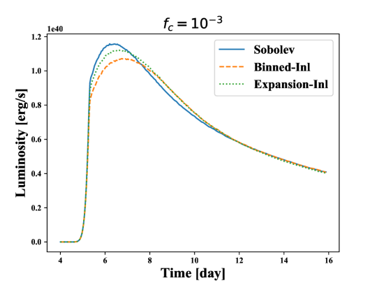
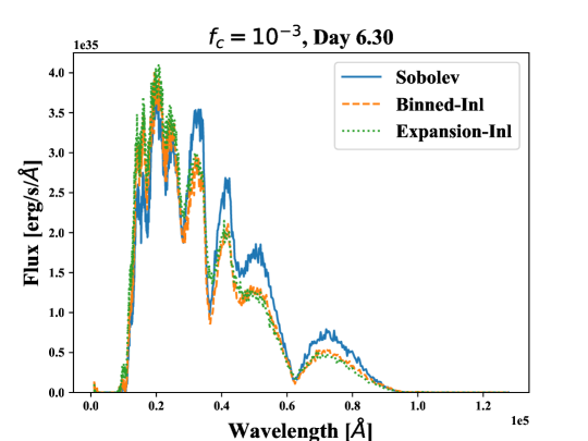
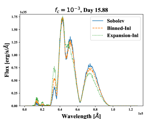
Figure 13: Bolometric luminosity (left panel) and radiative flux at 6.3 days (middle panel) and 15.88 days (right panel) for the simplified test problem described in the text. Results are shown for the continuous Monte Carlo Sobolev (solid blue), line-binned (dashed orange), and expansion-opacity (dotted green) methods. For consistency, these methods all employ line contributions to the opacity that were generated within the SuperNu code, rather than via the pre-tabulated approach. Also, an oscillator strength cutoff value of $f_{c}=10^{-3}$ was used in all cases.

4.2.2 Full problem: sensitivity studies

For the full problem, the time span is extended, ranging from $10^{4}$ seconds to 20 days in the comoving frame ($\sim 14$ observer days), with 400 logarithmically spaced time steps. All opacity contributions are included as well. We vary the parameters of this problem to examine how light curves and spectra are affected by changes to the opacity data and opacity discretization method. The variations include: group averaging methods (line-smeared versus line-binned versus expansion-opacity), number of photon energy groups, tabulated versus inline-generated opacities, oscillator strength cutoff value, atomic physics model (semi-relativistic versus fully relativitistic variants), and choice of element. As mentioned in the previous section, use of the direct Sobolev treatment is impractical in simulations of the full problem and therefore is not considered in the present analysis.

Figure 14 displays a comparison of the bolometric luminosity and spectra, at 5.45 days post-merger, calculated with line-binned and line-smeared opacities, both computed with the tabular approach. These results were calculated with 100 energy groups, which is the same resolution used in our detailed study of kilonovae light curves and spectra (Wollaeger et al., 2018). The good agreement between the two calculations indicates that the line-smeared approach used in that detailed study produces similar results to the currently proposed line-binned approach at this group resolution.

In Figure 15, we next present a group resolution study by displaying line-binned results computed with 100 and 1,024 groups. Once again, bolometric luminosities are presented in the left panel and spectra, at 5.45 days post-merger, are presented in the right panel. In this case, we see a difference of about 25% in the peak luminosity indicating that the higher number of groups is required to obtain better convergence. Significant differences are also observed in the spectra displayed in the right panel of this figure, providing further evidence that 100 groups is not generally sufficient to produce converged spectra. This lower group resolution is a deficiency of Wollaeger et al. 2018, but does not significantly impact the conclusions of that work. Firstly, the primary goal of that effort was to establish variations in the kilonova signal with respect to changes in morphology, composition, and $r$-process heating. The group resolution does not affect those trends. Additionally, the authors showed that 100 groups is virtually converged for the model with mixed dynamical ejecta composition (see Figure 7 in Wollaeger et al. 2018). That particular model was used in their section on detection prospects, and all dependent works. The 1,024 groups represent the standard resolution chosen for the test-problem simulations considered in this work and have been found to produce converged results. For completeness, we note that additional calculations with 4,096 groups were carried out (not shown) and the resulting light curves and spectra agreed well with those produced with 1,024 groups.

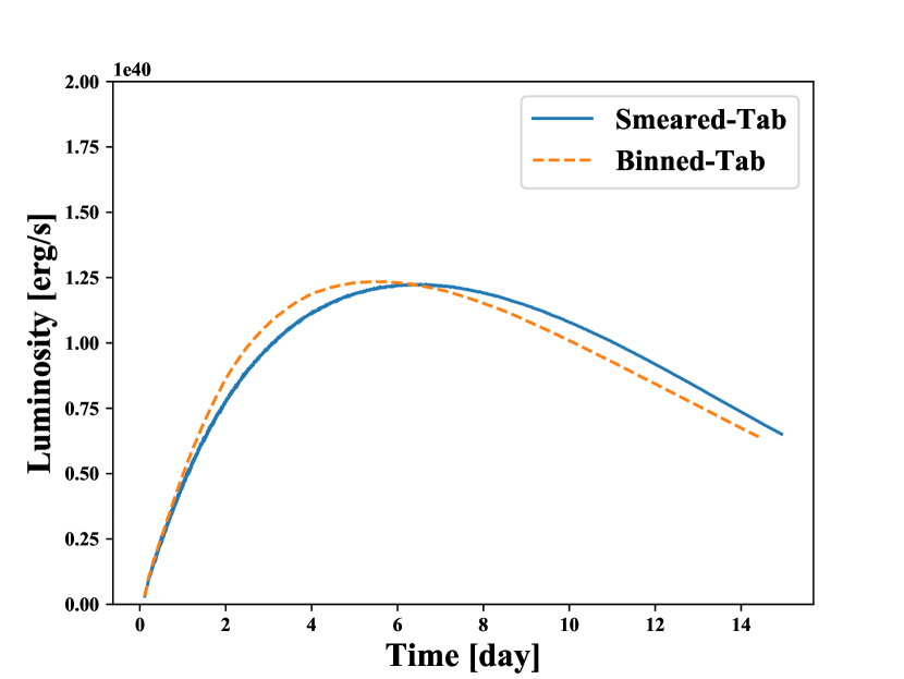
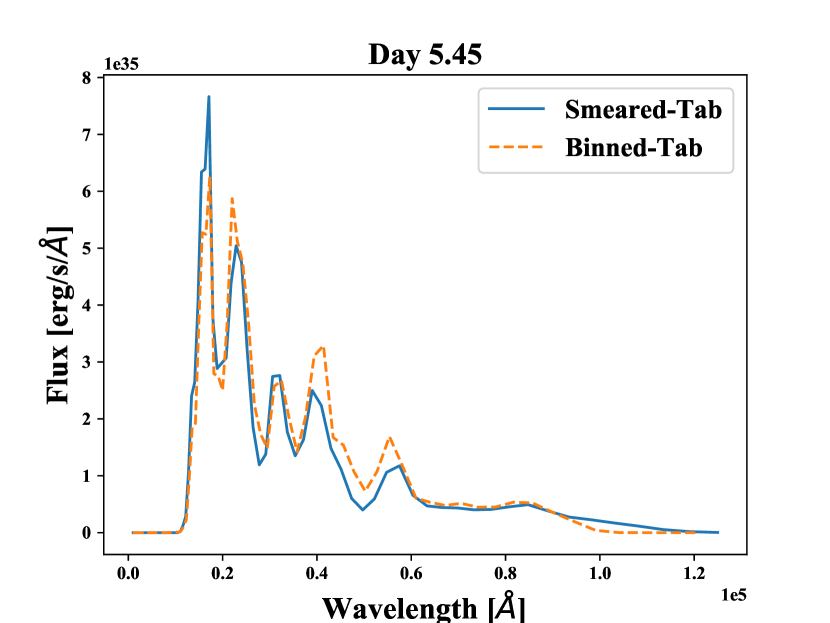
Figure 14: For the Nd ejecta test problem, a comparison of bolometric luminosities and spectra, at 5.45 days post-merger, computed with line-smeared (solid blue curve) and line-binned (dashed orange curve) opacities. These results were computed with 100 groups, consistent with the simulations of Wollaeger et al. 2018.

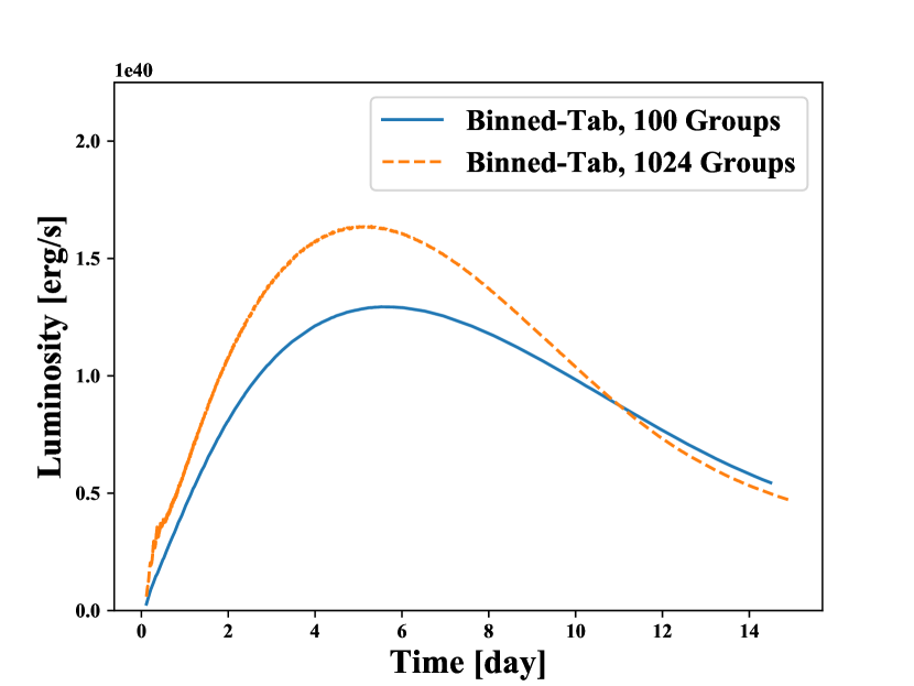
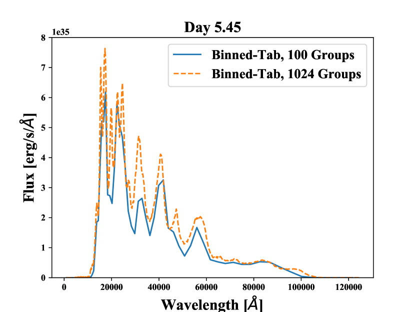
Figure 15: For the Nd ejecta test problem, a comparison of bolometric luminosities and spectra, at 5.45 days post-merger, computed with line-binned opacities. Results are presented for 100 (solid blue curve) and 1,024 (dashed orange curve) groups.

We have also compared the fully tabulated, line-binned approach to the corresponding inline multigroup implementation, which solves the Saha-Boltzmann equations using the actual ejecta temperatures and densities. As mentioned previously, in the fully tabulated approaches (both smeared and binned), the opacity is instead obtained within SuperNu by interpolation on a precomputed density-temperature table, which can introduce some inaccuracy. Figure 16 displays the bolometric luminosity and spectra for tabulated versus inline, line-binned calculations. The good agreement between these two sets of calculations indicates that potential errors arising from interpolation of the tabular bound-bound opacities are insignificant, and, furthermore, that the method for distributing the tabular, line-binned opacities across group boundaries (see Section 2.1) is adequate.

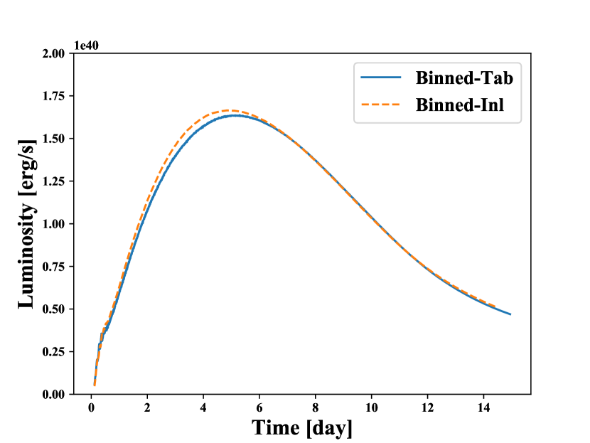
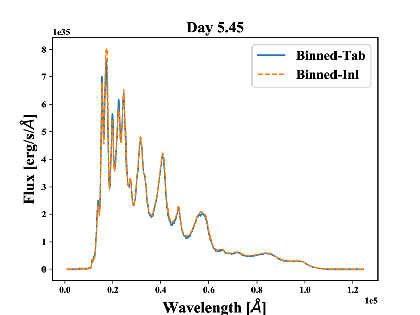
Figure 16: Comparison of tabulated (solid blue curve) and inline (dashed orange curve), line-binned opacity implementations. Figures 16 and 16 display luminosities and spectra, respectively. The good agreement between these two implementations indicates that our method for processing the tabular opacity data does not introduce any significant error in the simulations.

We next investigated the sensitivity of the emission to the oscillator strength cutoff value, $f_{c}$. Figures 17 and 18 display plots of light curves and spectra, respectively, for different oscillator strength cutoffs. Each panel contains two curves that were generated with the inline, line-binned and expansion-opacity methods. Results are shown for cutoff values of $f_{c}\in\{10^{-1},10^{-3},10^{-4},10^{-6}\}$. These four cutoffs correspond to including a total of 2,814, 1,225,925, 6,447,337, and 22,710,094 lines, respectively. These results indicate that the opacity changes significantly when lowering $f_{c}$ from $10^{-1}$ to $10^{-3}$, but the effect of including additional lines appears to level off at $10^{-4}$, which is consistent with the behavior exhibited by the opacity curves in the earlier Figure 11. We also note that the same convergence behavior is exhibited for both the line-binned and expansion-opacity methods, although the light curves and spectra display some quantitative differences, even for the most inclusive atomic model generated with $f_{c}=10^{-6}$. For example, there is about a 30% difference in the peak luminosity when comparing expansion-opacity and line-binned light curves for this full problem, versus only 5% mentioned in the previous section for the simplified problem. However, we again note that these disparities are not sufficient to explain discrepancies between theory and observation.

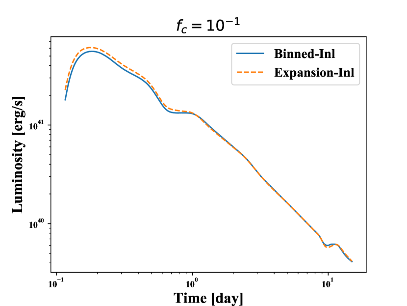
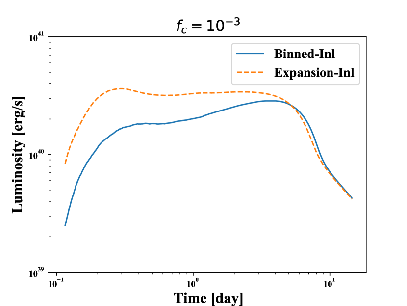
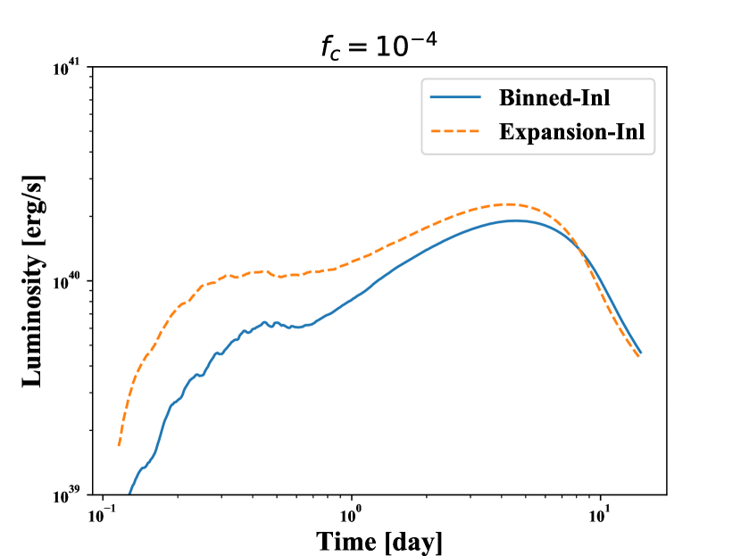
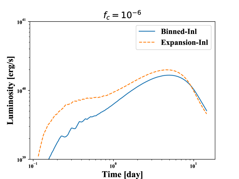
Figure 17: Bolometric luminosity for oscillator strength cutoff values of $f_{c}=10^{-1}$, $10^{-3}$, $10^{-4}$, and $10^{-6}$ in Figures 17, 17, 17 and 17, respectively. Results are presented for line-binned (solid blue curve) and expansion (dashed orange curve) inline opacities. There is a relatively strong dependence on $f_{c}$ down to a value of $10^{-4}$, below which the light curves do not change too much.

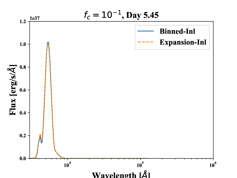
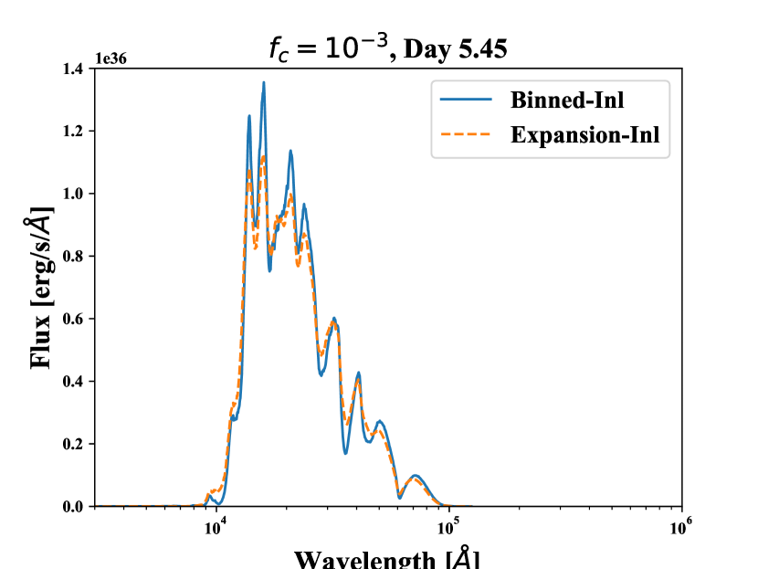
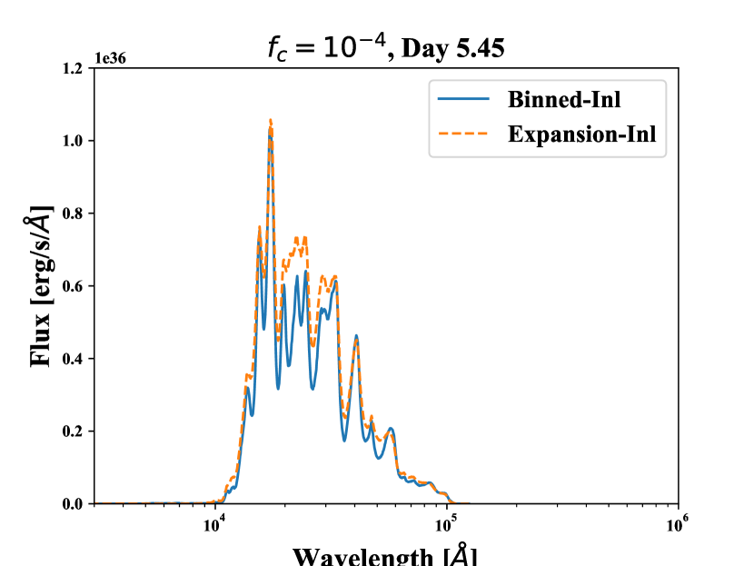
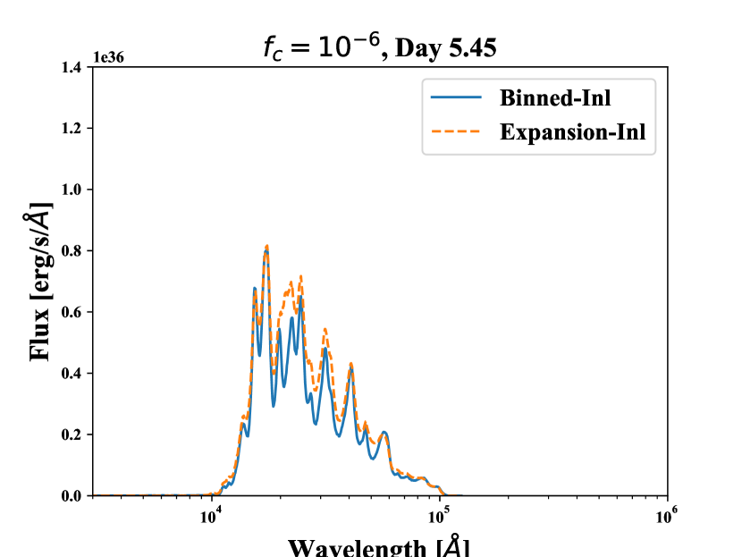
Figure 18: Spectra at day 5.45 for oscillator strength cutoff values of $f_{c}=10^{-1}$, $10^{-3}$, $10^{-4}$, and $10^{-6}$ in Figures 18, 18, 18 and 18, respectively. Results are presented for line-binned (solid blue curve) and expansion (dashed orange curve) inline opacities. There is a strong dependence on $f_{c}$ down to a value of $10^{-4}$, with significant differences still occurring in certain line features for the most complete model with $f_{c}=10^{-6}$.

In Figure 19, we compare light curves using either semi-relativistic (SR) or fully relativistic (FR) atomic data, and either the line-binned or expansion-opacity method. The bolometric luminosities (left panel) agree reasonably well between opacity discretization methods, but the spectra agree better between the two types of atomic data. Figure 20 displays light curves and spectra for the FR-SCR and FR-SCNR variants of the FR model, which have less fidelity, i.e. less configuration interaction, than the default FR model. Unlike the SR versus FR comparison in Figure 19, the bolometric luminosities do not group together according to the opacity discretization method, near peak luminosity. This behavior indicates a stronger sensitivity to the amount of fine-structure detail that is included in the atomic physics models, relative to a sensitivity to the discretization method. Additionally, the FR-SCNR light curves and spectra are more closely in agreement with those of the FR and SR models, which is consistent with theoretical expectations (see Section 2.3 and Table 2).

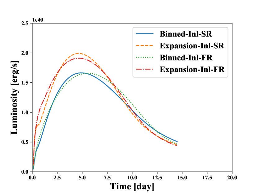
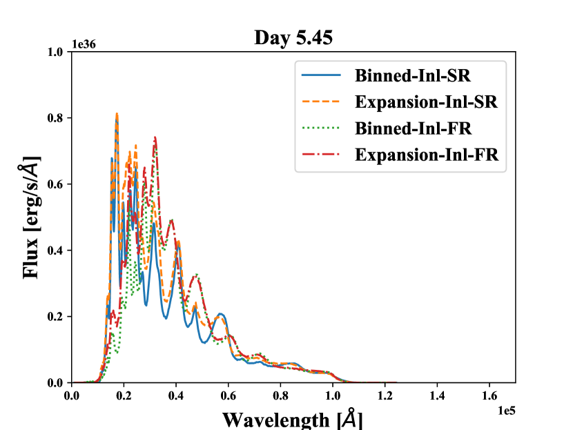
Figure 19: Comparison of line-binned and expansion-opacity results using semi-relativistic (SR) and fully relativistic (FR) atomic data to calculate opacities. Figures 19 and 19 display luminosities and spectra, respectively.

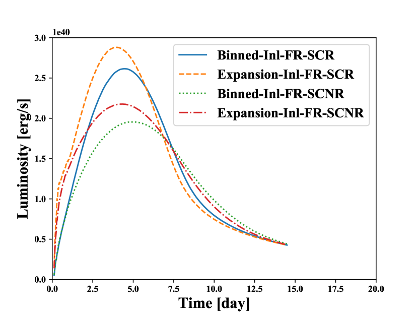
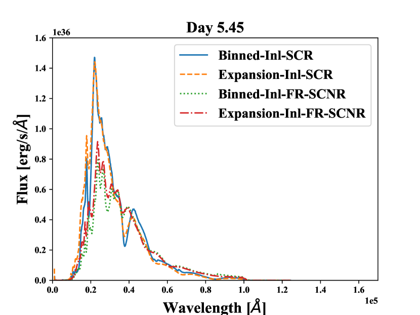
Figure 20: Comparison of line-binned and expansion opacity results using the different configuration-interaction variations of FR atomic data (SCR and SCNR) to calculate opacities. Figures 20 and 20 display luminosities and spectra, respectively.

It is interesting to note that the spectral responses to the above suite of parameter variations do not show significant shifts in the wavelength band at which peak emission occurs. This suggests that the area-preserving opacity technique, and these other numerical resolution choices employed in our earlier work (Wollaeger et al., 2018), do not appear to explain why the spectra presented therein is shifted toward red wavelengths, as compared to results produced by other authors who use the expansion-opacity treatment (e.g. Kasen et al. 2017; Tanaka et al. 2018). Clearly, the parameter study presented here is not exhaustive and further methodical, sensitivity studies of other key properties will be needed (e.g. ejecta characteristics such as density, elemental composition and velocity distributions, as well as details in the atomic data employed by each group). As discussed in Section 4.2.1, simplified test problems provide a valuable path to isolating the impact of various assumptions employed by the full kilonova modeling codes, and future work should attempt to define such tests.

It is also worth noting that there is a common assumption among all groups that the opacity contribution from the mixing of heavy elements present in the ejecta can be reasonably represented by a surrogate, single-element lanthanide (Nd is commonly assumed). By considering different elements here, we demonstrate that the choice of element can have a significant impact on the light curves and spectra as well. Figure 21 displays bolometric luminosity for line-binned opacity tables of Nd along with Sm, Ce, and U. Sm and Ce differ from Nd in atomic number by only +2 and -2, respectively, but produce significantly brighter light curves, by about a factor of two at 5.45 days post-merger. Moreover, Ce has a bright early transient for both SR and FR opacity, presumably due to its relatively low opacity that results from a smaller number of $4f$ electrons. Nd and U are homologues, i.e. they appear in the same column of the periodic table due to the similar electron structure (with the principal quantum number of their valence shells differing by one), but U displays a peak luminosity that is about five times brighter and appears earlier by about three days. The corresponding spectra for these four elements are presented in Figure 22. The peak emission varies in value by about a factor of 2.5 for the SR calculations and a factor of 4.3 for the FR calculations, and its wavelength location ranges from $\sim$10,000–30,000 Å. This type of sensitivity indicates that using a more complete set of lanthanide elements to simulate kilonovae, rather than a single representative element, may be appropriate.

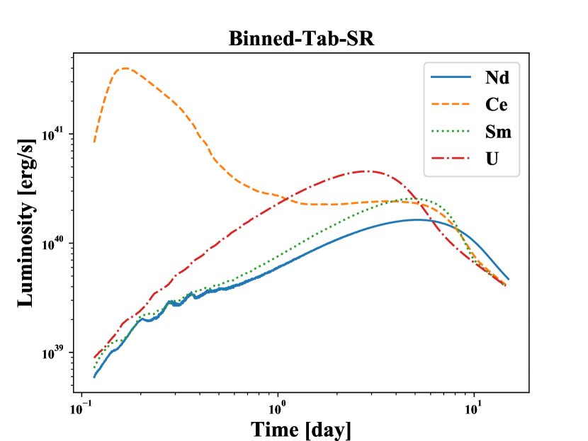
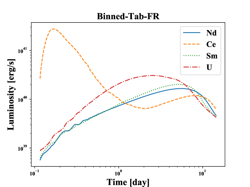
Figure 21: Bolometric luminosity for different elements: Nd (blue solid), Ce (orange dashed), Sm (green dotted), and U (red dot-dashed) using tabulated semi-relativistic (left panel) or fully relativistic (right panel) binned opacities.

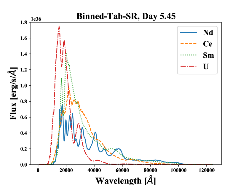
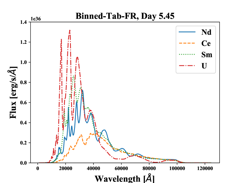
Figure 22: Spectra at 5.45 days for different elements: Nd (blue solid), Ce (orange dashed), Sm (green dotted), and U (red dot-dashed) using tabulated semi-relativistic (left panel) or fully relativistic (right panel) binned opacities.

Finally, we provide some basic timing information to demonstrate the efficiency of the tabular, line-binned opacity method compared to the corresponding inline approach, when simulating kilonovae emission. For the case of $f_{c}=10^{-6}$, SR atomic data and pure Nd, the total time, in seconds, spent in the opacity calculations per MPI rank is: 0.1162 for tabular line-binned (“Binned-Tab”), 167.001 for inline line-binned (“Binned-Inl”) and 284.538 for expansion-opacity (“Expansion-Inl”). (For reference, in our simulations the total mean time spent in the radiation transport logic, for $\sim 10^{6}$ particles per MPI rank, is 1060.51 s.) Thus, the tabular approach is approximately three orders of magnitude faster than the inline approach due to the amount of time required to obtain the atomic level populations and to construct the line-binned opacities for every required temperature-density. Also of note is the fact that the inline expansion-opacity calculation requires a factor of 1.7 more time than the corresponding line-binned calculation. The additional cost in the expansion-opacity method is due to the evaluation of the exponentials for each line.

5 Summary

We have proposed an area-preserving (line-binned), tabular approach for calculating opacities relevant to the modeling of kilonova light curves and spectra. The line-binned approach is superior to the previous line-smeared approach because the former is guaranteed to preserve the integral of the opacity. The area-preserving approach differs from the more widely employed expansion-opacity method in how the line contribution to the opacity is calculated. However, our alternative approach was demonstrated to produce similar emission results compared to both the expansion-opacity method and to the more accurate, direct implementation of Sobolev line transfer for a simplified problem (see Figure 13). In fact, light curves produced by the approximate line-binned and expansion-opacity methods were found to be lower than the direct Sobolev treatment by a maximum of 8% and 3%, respectively. As expected, our line-binned light curve is less than or equal to the expansion-opacity light curve, with a maximum difference of 5% occurring at peak for the simplified test case. The spectral features show greater variability in the level of agreement between the three opacity implementations, with our line-binned approach agreeing well with the direct line treatment at late times.

We considered a more complete (“full”) problem to study the errors associated with choices for the oscillator strength cutoff value, $f_{c}$, which determines the number of lines that are used in a particular simulation (see Figures 17, 18), as well as sensitivities to the use of variant FR and SR atomic models (see Figures 19, 20). We found that light curves are typically converged at a value of $f_{c}=10^{-4}$. Increasing the cutoff value by one order of magnitude, $f_{c}=10^{-3}$, results in a 50% error in the peak of the curve and a factor of three or so in the early-time behavior. For the converged light curves produced with this full problem, a larger difference of about 30% was obtained in the peak luminosity when comparing expansion-opacity and line-binned simulations. Obtaining convergence for all major spectral features typically required a lower tolerance of $f_{c}=10^{-6}$. As for SR versus FR models, the light curves were found to be relatively insensitive to this option, but certain spectral features displayed visible differences, and the FR calculation produced emission that is shifted toward slightly higher (redder) wavelengths.

The choice of element comprising the ejecta was also investigated and found to be a significant factor in predictions of the brightness and shape of the bolometric luminosity light curve, as well as the corresponding spectra, for single-element simulations. (see Figures 21 and 22). The peak luminosity varied by factors of 2–5 when considering lanthanides and an actinide with several $f$-shell valence electrons in the ground state of their neutral ion stages. The magnitude of the peak spectral emission differed by similar amounts, i.e. factors of 2.5–4.3. A study of the relative importance of various elements in multi-element light-curve and spectral simulations is reserved for future work.

From a practical, computational perspective, the tabular line-binned approach presented here is more efficient than the traditional expansion-opacity method because the opacities are independent of the particular type of expansion and can therefore be precomputed on a grid of temperatures and densities. It was found that the tabular approach requires three orders of magnitude less time than the expansion-opacity method to generate the relevant opacities for typical kilonova simulations. Tabular opacities for all 14 lanthanide elements, as well as for a representative actinide element, uranium, have been generated using the line-binned approach. These data are currently available, by request, from the corresponding author and we plan to make them publicly available via a new database developed in collaboration with NIST.

Appendix A List of configurations used in this work

Table 4 in this appendix contains a list of configurations that were used in calculating the energy levels and oscillator strengths for the 14 lanthanide elements and sole actinide (uranium) element considered in this work. Based on the relevant conditions of kilonova ejecta, only the first four ion stages were calculated for each element. The list of configurations was chosen to obtain a good representation of the lowest lying energy levels that are necessary to: (a) obtain converged atomic level populations via Saha-Boltzmann statistics and (b) calculate converged opacities with respect to the number of bound-bound transitions in the photon energy range of interest. The choice of configurations was based on the energy-level entries in the NIST database (Kramida et al., 2018) as well as ab initio atomic structure calculations.

Table 4: A list of configurations, number of fine-structure levels, and number of (electric dipole) absorption lines for the various ion stages considered in this work. A completely filled Xe core is assumed for the 14 lanthanide elements, while a filled Rn core is assumed for uranium. For the first two ion stages of ytterbium, Yb i and ii, the orbital angular momentum symbol $\ell$ represents the range of values $\ell=s,p,d,f$ and $g$.

Ion stage	Configurations	# of levels	# of lines
La i	$5d^{1}6s^{2}$, $5d^{2}6s^{1}$, $5d^{3}$, $5d^{1}6s^{1}6p^{1}$, $4f^{1}6s^{2}$, $6s^{2}6p^{1}$,	366	16,163
	$5d^{2}6p^{1}$, $4f^{1}5d^{1}6s^{1}$, $4f^{1}6s^{1}6p^{1}$, $4f^{1}5d^{2}$, $4f^{1}5d^{1}6p^{1}$
La ii	$5d^{2}$, $5d^{1}6s^{1}$, $4f^{1}6s^{1}$, $6s^{2}$, $4f^{1}5d^{1}$,	79	768
	$5d^{1}6p^{1}$, $6s^{1}6p^{1}$, $4f^{1}6p^{1}$, $4f^{2}$
La iii	$5d^{1}$, $4f^{1}$, $6s^{1}$, $6p^{1}$	7	8
La iv	$5p^{6}$, $5p^{5}4f^{1}$, $5p^{5}6s^{1}$, $5p^{5}5d^{1}$, $5p^{5}6p^{1}$	39	211
Ce i	$4f^{2}6s^{2}$, $4f^{1}5d^{1}6s^{2}$, $4f^{1}5d^{2}6s^{1}$, $4f^{1}5d^{1}6s^{1}6p^{1}$, $4f^{2}5d^{1}6s^{1}$,	2,546	626,112
	$4f^{2}6s^{1}6p^{1}$, $4f^{1}5d^{3}$, $4f^{1}6s^{2}6p^{1}$, $4f^{1}5d^{2}6p^{1}$, $4f^{2}5d^{2}$, $4f^{2}5d^{1}6p^{1}$
Ce ii	$4f^{2}6s^{1}$, $4f^{2}5d^{1}$, $4f^{2}6p^{1}$, $4f^{1}5d^{2}$, $4f^{1}6s^{2}$,	519	28,887
	$4f^{1}5d^{1}6s^{1}$, $4f^{1}5d^{1}6p^{1}$, $4f^{1}6s^{1}6p^{1}$, $5d^{3}$, $4f^{3}$
Ce iii	$4f^{2}$, $4f^{1}6s^{1}$, $4f^{1}5d^{1}$, $4f^{1}6p^{1}$, $5d^{2}$, $5d^{1}6s^{1}$	62	452
Ce iv	$4f^{1}$, $6s^{1}$, $5d^{1}$, $6p^{1}$	7	8
Pr i	$4f^{3}6s^{2}$, $4f^{2}5d^{1}6s^{2}$, $4f^{2}5d^{2}6s^{1}$, $4f^{3}5d^{1}6s^{1}$,	7,362	4,750,354
	$4f^{3}5d^{2}$, $4f^{2}5d^{1}6s^{1}6p^{1}$, $4f^{3}5d^{1}6p^{1}$, $4f^{3}6s^{1}6p^{1}$
Pr ii	$4f^{3}6s^{1}$, $4f^{3}5d^{1}$, $4f^{3}6p^{1}$, $4f^{2}5d^{2}$,	2,145	412,027
	$4f^{2}5d^{1}6s^{1}$, $4f^{2}5d^{1}6p^{1}$, $4f^{2}6s^{1}6p^{1}$
Pr iii	$4f^{3}$, $4f^{2}6s^{1}$, $4f^{2}5d^{1}$,	361	12,394
	$4f^{2}6p^{1}$, $4f^{1}5d^{2}$, $4f^{1}5d^{1}6s^{1}$
Pr iv	$4f^{2}$, $4f^{1}6s^{1}$, $4f^{1}5d^{1}$, $4f^{1}6p^{1}$	49	296
Nd i	$4f^{4}6s^{2}$, $4f^{3}5d^{1}6s^{2}$, $4f^{4}5d^{1}6s^{1}$, $4f^{4}5d^{2}$,	18,104	25,224,451
	$4f^{3}5d^{1}6s^{1}6p^{1}$, $4f^{4}5d^{1}6p^{1}$, $4f^{4}6s^{1}6p^{1}$
Nd ii	$4f^{4}6s^{1}$, $4f^{4}5d^{1}$, $4f^{4}6p^{1}$, $4f^{3}5d^{2}$,	6,888	3,958,977
	$4f^{3}5d^{1}6s^{1}$, $4f^{3}5d^{1}6p^{1}$, $4f^{3}6s^{1}6p^{1}$
Nd iii	$4f^{4}$, $4f^{3}6s^{1}$, $4f^{3}5d^{1}$, $4f^{3}6p^{1}$,	1,650	233,822
	$4f^{2}5d^{2}$, $4f^{2}5d^{1}6s^{1}$, $4f^{1}5d^{2}6s^{1}$
Nd iv	$4f^{3}$, $4f^{2}6s^{1}$, $4f^{2}5d^{1}$, $4f^{2}6p^{1}$	241	5,784
Pm i	$4f^{5}6s^{2}$, $4f^{4}5d^{1}6s^{2}$, $4f^{5}5d^{1}6s^{1}$, $4f^{5}5d^{2}$,	37,504	102,137,397
	$4f^{4}5d^{1}6s^{1}6p^{1}$, $4f^{5}5d^{1}6p^{1}$, $4f^{5}6s^{1}6p^{1}$
Pm ii	$4f^{5}6s^{1}$, $4f^{5}5d^{1}$, $4f^{5}6p^{1}$, $4f^{4}5d^{2}$,	16,595	21,306,571
	$4f^{4}5d^{1}6s^{1}$, $4f^{4}5d^{1}6p^{1}$, $4f^{4}6s^{1}6p^{1}$
Pm iii	$4f^{5}$, $4f^{4}6s^{1}$, $4f^{4}5d^{1}$, $4f^{4}6p^{1}$,	5,274	2,262,145
	$4f^{3}5d^{2}$, $4f^{3}5d^{1}6s^{1}$, $4f^{2}5d^{2}6s^{1}$
Pm iv	$4f^{4}$, $4f^{3}6s^{1}$, $4f^{3}5d^{1}$, $4f^{3}6p^{1}$	817	57,765
Sm i	$4f^{6}6s^{2}$, $4f^{5}5d^{1}6s^{2}$, $4f^{6}5d^{1}6s^{1}$, $4f^{6}5d^{2}$,	60,806	249,301,825
	$4f^{5}5d^{1}6s^{1}6p^{1}$, $4f^{6}5d^{1}6p^{1}$, $4f^{6}6s^{1}6p^{1}$
Sm ii	$4f^{6}6s^{1}$, $4f^{6}5d^{1}$, $4f^{6}6p^{1}$, $4f^{5}5d^{2}$,	29,970	67,743,385
	$4f^{5}5d^{1}6s^{1}$, $4f^{5}5d^{1}6p^{1}$, $4f^{5}6s^{1}6p^{1}$
Sm iii	$4f^{6}$, $4f^{5}6s^{1}$, $4f^{5}5d^{1}$, $4f^{5}6p^{1}$,	13,170	13,318,114
	$4f^{4}5d^{2}$, $4f^{4}5d^{1}6s^{1}$, $4f^{3}5d^{2}6s^{1}$
Sm iv	$4f^{5}$, $4f^{4}6s^{1}$, $4f^{4}5d^{1}$, $4f^{4}6p^{1}$	1,994	320,633
Eu i	$4f^{7}6s^{2}$, $4f^{6}5d^{1}6s^{2}$, $4f^{7}5d^{1}6s^{1}$, $4f^{7}5d^{2}$, $4f^{6}5d^{2}6s^{1}$, $4f^{6}5d^{1}6s^{1}6p^{1}$,	110,887	902,515,995
	$4f^{7}5d^{1}6p^{1}$, $4f^{7}6s^{1}6p^{1}$, $4f^{7}6s^{1}6d^{1}$, $4f^{7}6s^{1}7s^{1}$, $4f^{7}6s^{1}7p^{1}$
Eu ii	$4f^{7}6s^{1}$, $4f^{7}5d^{1}$, $4f^{7}6p^{1}$, $4f^{6}5d^{2}$, $4f^{6}5d^{1}6s^{1}$,	46,213	152,795,763
	$4f^{6}5d^{1}6p^{1}$, $4f^{6}6s^{1}6p^{1}$, $4f^{7}6d^{1}$, $4f^{7}7s^{1}$
Eu iii	$4f^{7}$, $4f^{6}6s^{1}$, $4f^{6}5d^{1}$,	17,058	13,844,004
	$4f^{6}6p^{1}$, $4f^{5}5d^{2}$, $4f^{5}5d^{1}6s^{1}$
Eu iv	$4f^{6}$, $4f^{5}6s^{1}$, $4f^{5}5d^{1}$, $4f^{5}6p^{1}$	3,737	1,045,697
Gd i	$4f^{8}6s^{2}$, $4f^{7}5d^{1}6s^{2}$, $4f^{7}5d^{2}6s^{1}$, $4f^{7}5d^{2}6p^{1}$, $4f^{7}6s^{2}6p^{1}$, $4f^{7}6s^{1}6p^{2}$,	228,048	3,583,266,975
	$4f^{7}5d^{3}$, $4f^{8}5d^{1}6s^{1}$, $4f^{8}5d^{2}$, $4f^{7}5d^{1}6s^{1}6p^{1}$, $4f^{8}5d^{1}6p^{1}$, $4f^{8}6s^{1}6p^{1}$
Gd ii	$4f^{8}6s^{1}$, $4f^{8}5d^{1}$, $4f^{8}6p^{1}$, $4f^{7}5d^{2}$, $4f^{7}6s^{2}$,	46,733	160,595,610
	$4f^{7}5d^{1}6s^{1}$, $4f^{7}5d^{1}6p^{1}$, $4f^{7}6s^{1}6p^{1}$
Gd iii	$4f^{8}$, $4f^{7}6s^{1}$, $4f^{7}5d^{1}$, $4f^{7}6p^{1}$,	39,324	113,346,746
	$4f^{6}5d^{2}$, $4f^{6}5d^{1}6s^{1}$, $4f^{5}5d^{2}6s^{1}$
Gd iv	$4f^{7}$, $4f^{6}6s^{1}$, $4f^{6}5d^{1}$, $4f^{6}6p^{1}$	5,323	2,073,701

Table 4: Continued…

Ion stage	Configurations	# of levels	# of lines
Tb i	$4f^{9}6s^{2}$, $4f^{8}5d^{1}6s^{2}$, $4f^{8}5d^{2}6s^{1}$, $4f^{8}6s^{2}6p^{1}$, $4f^{9}5d^{1}6s^{1}$,	84,779	530,258,427
	$4f^{9}5d^{2}$, $4f^{8}5d^{1}6s^{1}6p^{1}$, $4f^{9}5d^{1}6p^{1}$, $4f^{9}6s^{1}6p^{1}$
Tb ii	$4f^{9}6s^{1}$, $4f^{9}5d^{1}$, $4f^{9}6p^{1}$, $4f^{8}6s^{2}$, $4f^{8}5d^{2}$,	40,502	120,186,078
	$4f^{8}5d^{1}6s^{1}$, $4f^{8}5d^{1}6p^{1}$, $4f^{8}6s^{1}6p^{1}$
Tb iii	$4f^{9}$, $4f^{8}6s^{1}$, $4f^{8}5d^{1}$, $4f^{8}6p^{1}$,	48,048	166,697,126
	$4f^{7}5d^{2}$, $4f^{7}5d^{1}6s^{1}$, $4f^{6}5d^{2}6s^{1}$
Tb iv	$4f^{8}$, $4f^{7}6s^{1}$, $4f^{7}5d^{1}$, $4f^{7}6p^{1}$	5,983	2,545,968
Dy i	$4f^{10}6s^{2}$, $4f^{9}5d^{1}6s^{2}$, $4f^{9}5d^{1}6s^{1}6p^{1}$, $4f^{10}5d^{1}6s^{1}$, $4f^{10}6s^{1}6p^{1}$, $4f^{10}6s^{1}6d^{1}$,	55,116	229,181,735
	$4f^{10}6s^{1}7s^{1}$, $4f^{10}6s^{1}7p^{1}$, $4f^{9}6s^{2}6p^{1}$, $4f^{9}5d^{2}6s^{1}$, $4f^{10}6p^{2}$, $4f^{10}5d^{1}6p^{1}$
Dy ii	$4f^{10}6s^{1}$, $4f^{10}5d^{1}$, $4f^{10}6p^{1}$, $4f^{9}5d^{2}$, $4f^{9}6s^{2}$,	26,968	55,381,943
	$4f^{9}5d^{1}6s^{1}$, $4f^{9}5d^{1}6p^{1}$, $4f^{9}6s^{1}6p^{1}$
Dy iii	$4f^{10}$, $4f^{9}6s^{1}$, $4f^{9}5d^{1}$,	20,834	12,685,641
	$4f^{9}6p^{1}$, $4f^{8}5d^{2}$, $4f^{8}5d^{1}6s^{1}$
Dy iv	$4f^{9}$, $4f^{8}6s^{1}$, $4f^{8}5d^{1}$, $4f^{8}6p^{1}$	5,194	1,943,961
Ho i	$4f^{11}6s^{2}$, $4f^{10}5d^{1}6s^{2}$, $4f^{10}5d^{1}6s^{1}6p^{1}$, $4f^{11}5d^{1}6s^{1}$, $4f^{11}6s^{1}6p^{1}$, $4f^{11}6s^{1}6d^{1}$,	26,759	57,149,392
	$4f^{11}6s^{1}7s^{1}$, $4f^{11}6s^{1}7p^{1}$, $4f^{10}6s^{2}6p^{1}$, $4f^{10}5d^{2}6s^{1}$, $4f^{11}6p^{2}$, $4f^{11}5d^{1}6p^{1}$
Ho ii	$4f^{11}6s^{1}$, $4f^{11}5d^{1}$, $4f^{11}6p^{1}$, $4f^{10}5d^{2}$, $4f^{10}6s^{2}$,	13,970	15,323,035
	$4f^{10}5d^{1}6s^{1}$, $4f^{10}5d^{1}6p^{1}$, $4f^{10}6s^{1}6p^{1}$
Ho iii	$4f^{11}$, $4f^{10}6s^{1}$, $4f^{10}5d^{1}$, $4f^{10}6p^{1}$	1,837	259,812
Ho iv	$4f^{10}$, $4f^{9}6s^{1}$, $4f^{9}5d^{1}$, $4f^{9}6p^{1}$	3,549	915,339
Er i	$4f^{12}6s^{2}$, $4f^{11}5d^{1}6s^{2}$, $4f^{11}5d^{1}6s^{1}6p^{1}$, $4f^{12}5d^{1}6s^{1}$, $4f^{12}6s^{1}6p^{1}$, $4f^{12}6s^{1}6d^{1}$,	9,904	8,223,793
	$4f^{12}6s^{1}7s^{1}$, $4f^{12}6s^{1}7p^{1}$, $4f^{11}6s^{2}6p^{1}$, $4f^{11}5d^{2}6s^{1}$, $4f^{12}6p^{2}$, $4f^{12}5d^{1}6p^{1}$
Er ii	$4f^{12}6s^{1}$, $4f^{12}5d^{1}$, $4f^{12}6p^{1}$, $4f^{11}5d^{2}$, $4f^{11}6s^{2}$,	5,333	2,432,666
	$4f^{11}5d^{1}6s^{1}$, $4f^{11}5d^{1}6p^{1}$, $4f^{11}6s^{1}6p^{1}$
Er iii	$4f^{12}$, $4f^{11}6s^{1}$, $4f^{11}5d^{1}$, $4f^{11}6p^{1}$	723	42,671
Er iv	$4f^{11}$, $4f^{10}6s^{1}$, $4f^{10}5d^{1}$, $4f^{10}6p^{1}$	1,837	259,812
Tm i	$4f^{13}6s^{2}$, $4f^{12}5d^{1}6s^{2}$, $4f^{12}5d^{1}6s^{1}6p^{1}$, $4f^{13}5d^{1}6s^{1}$, $4f^{13}6s^{1}6p^{1}$,	1,684	155,754
	$4f^{13}6s^{1}6d^{1}$, $4f^{13}6s^{1}7s^{1}$, $4f^{13}6s^{1}7p^{1}$, $4f^{12}6s^{2}6p^{1}$, $4f^{13}6p^{2}$, $4f^{13}5d^{1}6p^{1}$
Tm ii	$4f^{13}6s^{1}$, $4f^{13}5d^{1}$, $4f^{13}6p^{1}$, $4f^{12}5d^{2}$, $4f^{12}6s^{2}$,	1,484	205,258
	$4f^{12}5d^{1}6s^{1}$, $4f^{12}5d^{1}6p^{1}$, $4f^{12}6s^{1}6p^{1}$
Tm iii	$4f^{13}$, $4f^{12}6s^{1}$, $4f^{12}5d^{1}$, $4f^{12}6p^{1}$	202	3,797
Tm iv	$4f^{12}$, $4f^{11}6s^{1}$, $4f^{11}5d^{1}$, $4f^{11}6p^{1}$	723	42,671
Yb i	$4f^{14}6s^{1}6\ell^{1}$, $4f^{14}6s^{1}7\ell^{1}$, $4f^{14}6s^{1}8\ell^{1}$, $4f^{14}6s^{1}9\ell^{1}$, $4f^{14}6s^{1}10\ell^{1}$, $4f^{14}6s^{1}11\ell^{1}$,	1,117	111,828
	$4f^{14}5d^{1}6s^{1}$, $4f^{14}5d^{1}6p^{1}$, $4f^{14}6s^{1}5f^{1}$, $4f^{14}6s^{1}5g^{1}$, $4f^{14}6p^{2}$, $4f^{14}5d^{2}$, $4f^{13}5d^{1}6s^{2}$,
	$4f^{13}5d^{2}6s^{1}$, $4f^{13}5d^{1}6s^{1}6p^{1}$, $4f^{13}6s^{2}6p^{1}$, $4f^{13}6s^{1}6p^{2}$, $4f^{13}6s^{2}6d^{1}$, $4f^{13}5d^{2}6p^{1}$
Yb ii	$4f^{14}6\ell^{1}$, $4f^{14}7\ell^{1}$, $4f^{14}8\ell^{1}$, $4f^{14}5d^{1}$, $4f^{14}5f^{1}$, $4f^{14}5g^{1}$,	292	9,673
	$4f^{13}5d^{2}$, $4f^{13}6s^{2}$, $4f^{13}5d^{1}6s^{1}$, $4f^{13}5d^{1}6p^{1}$, $4f^{13}6s^{1}6p^{1}$
Yb iii	$4f^{14}$, $4f^{13}6s^{1}$, $4f^{13}5d^{1}$, $4f^{13}6p^{1}$, $4f^{13}6d^{1}$, $4f^{13}6f^{1}$,	171	3,192
	$4f^{13}5f^{1}$, $4f^{13}7s^{1}$, $4f^{13}7p^{1}$, $4f^{13}7d^{1}$, $4f^{13}7f^{1}$
Yb iv	$4f^{13}$, $4f^{12}6s^{1}$, $4f^{12}5d^{1}$, $4f^{12}6p^{1}$	202	3,797
U i	$5f^{4}7s^{2}$, $5f^{3}6d^{1}7s^{2}$, $5f^{4}6d^{1}7s^{1}$,	16,882	20,948,831
	$5f^{4}6d^{2}$, $5f^{3}6d^{1}7s^{1}7p^{1}$, $5f^{4}6d^{1}7p^{1}$
U ii	$5f^{3}7s^{2}$, $5f^{4}7s^{1}$, $5f^{4}6d^{1}$, $5f^{4}7p^{1}$,	6,929	4,016,742
	$5f^{3}6d^{2}$, $5f^{3}6d^{1}7s^{1}$, $5f^{3}6d^{1}7p^{1}$, $5f^{3}7s^{1}7p^{1}$
U iii	$5f^{4}$, $5f^{3}7s^{1}$, $5f^{3}6d^{1}$, $5f^{3}7p^{1}$,	1,650	233,822
	$5f^{2}6d^{2}$, $5f^{2}6d^{1}7s^{1}$, $5f^{1}6d^{2}7s^{1}$
U iv	$5f^{3}$, $5f^{2}7s^{1}$, $5f^{2}6d^{1}$, $5f^{2}7p^{1}$	241	5,784

Appendix B Sobolev implementation in the SuperNu code

In this appendix, we discuss the implementation of a direct Sobolev treatment in the SuperNu code. To do so, we write down the equations and describe details of the algorithm.

The Sobolev method needs to be made compatible with Implicit Monte Carlo (IMC, Fleck & Cummings (1971)). Consequently, it is instructive to revisit the basic equations implemented in SuperNu, which like the SEDONA code, assumes the homologous approximation (Kasen et al., 2006),

$$\vec{v}=\frac{\vec{r}}{t}\;\;,$$ (10)

where $\vec{v}$ is velocity and $t$ is time. Incorporating Equation (10) into the $O(v/c)$ transport equation gives (see, for instance, Castor (2004))

$$\frac{1}{c}\frac{D\psi}{Dt}+\hat{\Omega}\cdot\nabla\psi+\frac{1}{ct}\lambda\frac{\partial\psi}{\partial\lambda}+\frac{3}{ct}\psi=j-\rho\kappa\psi\;,$$ (11)

where $\hat{\Omega}$ is the direction unit vector, $\lambda$ is wavelength, $\psi$ is angular intensity, $j$ is emissivity, and $\kappa$ is opacity. All quantities, except the spatial coordinate and time, are evaluated in the comoving frame. The corresponding IMC formulation requires an equation for the internal energy (or temperature of the matter). Assuming LTE, after performing a linear temporal expansion in $T^{4}$ of the Lagrangian internal energy equation (Fleck & Cummings, 1971), the IMC equations in SuperNu are

$$\frac{1}{c}\frac{D\psi}{Dt}+\hat{\Omega}\cdot\nabla\psi+\frac{1}{ct_{n}}\lambda\frac{\partial\psi}{\partial\lambda}+\frac{3}{ct_{n}}\psi=$$

$$\qquad\qquad f_{n}\rho_{n}\kappa_{n}B_{n}+\frac{b_{n}\kappa_{n}}{4\pi\kappa_{P,n}}(1-f_{n})$$

$$\qquad\qquad\times\int_{4\pi}d\Omega^{\prime}\int_{0}^{\infty}d\lambda^{\prime}\rho_{n}\kappa_{n}^{\prime}\psi^{\prime}-f_{n}\rho_{n}\kappa_{n}\psi\;,$$ (12a)

$$\rho_{n}c_{v,n}\frac{DT}{Dt}=\rho_{n}f_{n}\int_{4\pi}d\Omega\int_{0}^{\infty}d\lambda(\kappa_{n}\psi-\kappa_{n}B_{n})\;,$$ (12b)

$$f_{n}=\frac{1}{1+c\Delta t_{n}\kappa_{P,n}4acT_{n}^{3}/c_{v,n}}\;,$$ (12c)

where quantities subscripted with $n$ are evaluated at the beginning of time step $n$, $f_{n}$ is the Fleck factor, $B$ is the Planck function $b$ is the normalized Planck function, $\kappa_{P}$ is the Planck opacity, and $c_{v}$ is heat capacity. For simplicity, we have neglected contributions from $r$-process decay and Thomson scattering (though generally speaking, these are included in the simulations). It is worth noting that the Fleck factor introduces an “effective scattering” term into the transport equation (the second term on the right-hand side of Equation (12a)). Monte Carlo particles undergoing an effective scattering event are thermally redistributed in their wavelengths (the $b_{n}\kappa_{n}/\kappa_{P,n}$ coefficient is the redistribution kernel).

In SuperNu, the opacity is typically discretized into groups in wavelength; these groups are defined in the comoving frame (local to each fluid parcel). However, the wavelength for Monte Carlo particles is left continuous. Consequently, the first two equations in Equation (12) become

$$\frac{1}{c}\frac{D\psi}{Dt}+\hat{\Omega}\cdot\nabla\psi+\frac{1}{ct_{n}}\lambda\frac{\partial\psi}{\partial\lambda}+\frac{3}{ct_{n}}\psi=$$

$$\qquad\qquad f_{n}\rho_{n}\kappa_{g,n}B_{g,n}+\frac{b_{g,n}\kappa_{g,n}}{4\pi\kappa_{P,n}}(1-f_{n})$$

$$\qquad\qquad\times\int_{4\pi}d\Omega^{\prime}\sum_{g^{\prime}}\rho_{n}\kappa_{g^{\prime},n}^{\prime}\psi^{\prime}-f_{n}\rho_{n}\kappa_{g,n}\psi\;,$$ (13a)

$$\rho_{n}c_{v,n}\frac{DT}{Dt}=\rho_{n}f_{n}\int_{4\pi}d\Omega\sum_{g}\left(\int_{g}d\lambda\kappa_{g,n}\psi-\kappa_{g,n}B_{g,n}\Delta\lambda_{g}\right)\;,$$ (13b)

where subscript $g$ denotes a group-averaged quantity, $b_{g}=\int_{g}d\lambda\;b/\Delta\lambda_{g}$, and the Planck opacity is evaluated via a sum over groups, $\kappa_{P}=\sum_{g}\kappa_{g}b_{g}$. Since the particle wavelength is left continuous, the particles Doppler shift continuously across groups as they stream through space. This particle behavior corresponds to having left the third term on the left-hand side of Equation (13a) to remain continuous in wavelength.

Alternatively, we may keep some of the opacity continuous in wavelength. To obtain the Sobolev formulation of the IMC equations, we simply substitute

$$\kappa_{n}=\tilde{\kappa}_{g,n}+\kappa_{n}^{b-b}$$ (14)

for $\kappa_{g,n}$ in Equations (13), where $\tilde{\kappa}_{g,n}$ are all continuum contributions (discretized into groups) and $\kappa_{n}^{b-b}$ is a monochromatic superposition of Dirac delta distributions corresponding to the line contributions. For our Sobolev test problem, we neglect $\tilde{\kappa}_{g,n}$.

For fully discrete opacity, we also discretize the bound-bound contribution, $\kappa_{n}^{b-b}\rightarrow\kappa_{g,n}^{b-b}$. Using the formulae from the paper,

$$\kappa_{g,n}^{b-b}=\frac{1}{\rho_{n}ct_{n}}\frac{1}{\Delta\lambda_{g}}\sum_{i\in\Delta\lambda_{g}}\begin{cases}\lambda_{i}\tau_{i},\text{for binned}\;,\\ \lambda_{i}(1-e^{-\tau_{i}}),\text{for expansion}\;,\end{cases}$$ (15)

where $i$ is a line index and $\tau_{i}$ is the corresponding Sobolev optical depth. It is straightforward to see that the expansion opacity formula reduces to the binned opacity formula for $\tau_{i}\ll 1$. It is also straightforward to see that the line-binned formula is in fact a direct integral-average of the monochromatic opacity over wavelength under the assumption that the line profiles are Dirac delta distributions:

$$\kappa_{g,n}^{b-b} = \frac{1}{\rho_{n}ct_{n}}\frac{1}{\Delta\lambda_{g}}\sum_{i\in\Delta\lambda_{g}}\lambda_{i}\tau_{i}$$ (16)

$$= \frac{1}{\rho_{n}ct_{n}}\frac{1}{\Delta\lambda_{g}}\sum_{i\in\Delta\lambda_{g}}t_{n}\frac{\pi e^{2}}{m_{e}c}N_{i}|f_{i}|\lambda_{i}^{2}$$

$$= \frac{1}{\rho_{n}}\frac{1}{\Delta\lambda_{g}}\sum_{i\in\Delta\lambda_{g}}\frac{\pi e^{2}}{m_{e}c^{2}}N_{i}|f_{i}|\lambda_{i}^{2}\;,$$

where $N_{i}$ is the number density of the initial level for line $i$ and $f_{i}$ is the oscillator strength.

B.1 Monte Carlo Algorithm with Discrete Opacity

The algorithm for the system of equations with fully discretized opacity (Equations (13)) is as follows:

1. Store particles from time step $n-1$, sample source particles in time step $n$:

   1. integrate first term on right-hand side of Equation (13a) in $\Omega$, sum over groups, and integrate over the volume of a spatial cell, then partition the energy across the prescribed number of source particles for the cell,

   2. sample each particle’s position in the cell, in time step $n$, and direction ($\hat{\Omega}$),

   3. sample each particle’s wavelength ($\lambda$) by first sampling the group from a cumulative distribution function (CDF) generated by $b_{g,n}\kappa_{g,n}/\kappa_{P,n}$, then uniformly within the sampled group.

2. Transport the updated set of particles. For each particle:

   1. Calculate the set of velocity distances (Kasen et al., 2006) to stream to each possible next particle event:

      $$d_{\rm es}=-\frac{\ln(\xi)}{t_{n}(1-f_{n})\rho_{n}\kappa_{g,n}}\;,$$ (17a)

      $$d_{\rm red}=c(\lambda_{g+1/2}-\lambda)/\lambda\;,$$ (17b)

      $$d_{b}=|\vec{r}_{b}(\hat{\Omega})-\vec{r}|\;,$$ (17c)

      $$d_{\rm end}=c(t_{n+1}-t)/t_{n}\;,$$ (17d)

      where $d_{\rm es}$, $d_{\rm red}$, $d_{b}$, and $d_{\rm end}$ are distances to effective scattering, redshift out of the group edge, the cell boundary along $\hat{\Omega}$, and to the end of time step $n$. The quantity $\xi\in[0,1]$ is a uniformly sampled random number.

   2. Select the event from the minimum distance $d$, and update the particle’s properties via streaming:

      $$t^{\prime}=t+\frac{t_{n}d}{c}\;,$$ (18a)

      $$\vec{r}^{\prime}=\vec{r}+d\hat{\Omega}\;,$$ (18b)

      $$E^{\prime}=Ee^{-(1-f_{n})\rho_{n}\kappa_{g,n}t_{n}d}\;,$$ (18c)

      $$\lambda^{\prime}=\lambda\left(1+\frac{d}{c}\right)\;,$$ (18d)

      where, for simplicity, the update to the spatial position has been written in Cartesian coordinates.

   3. Add $E(1-e^{-(1-f_{n})\rho_{n}\kappa_{g,n}t_{n}d})$ to the tally of absorbed energy in the time step.

   4. If the particle effectively scatters, sample $\hat{\Omega}$ isotropically and resample $\lambda$ thermally from $b_{g,n}\kappa_{g,n}/\kappa_{P,n}$.

   5. If the particle redshifts out of the group, set $g$ to $g+1$ for the next round of distance calculations.

   6. If the particle crosses the cell boundary, use the adjacent cell’s properties for the next round of distance calculations. If the edge of the simulation grid is reached, tally the particle as escaping flux for the observables (light curves and spectra).

   7. If the particle reaches the end of the time step, stop transporting and store it for $n+1$.

3. Account for redshift on particle energy weights using operator-split equation (Abdikamalov et al., 2012),

   $$\frac{\partial\psi}{\partial t}+\frac{\psi}{t_{n}}=0\;,$$ (19)

   which has solution $E^{\prime\prime}=E^{\prime}e^{-\Delta t_{n}/t_{n}}$ for each particle energy weight.

4. With the energy absorption tallied during the transport of the particles, update the internal energy of the ejecta with Equation (13b) (the absorbed energy tally is represented by the term with $\psi$ on the right-hand side).

The above algorithm applies to both expansion and line-binned opacity treatements. The only difference between the approaches to treating line-binned and expansion opacity is in how the bound-bound contribution of $\kappa_{n,g}$ is calculated (in Equation (15)). Again, Equation (15) shows that the expansion and line-binned opacity methods approach one another when $\tau_{i}\ll 1$.

B.2 Monte Carlo Algorithm with Sobolev Line Treatment

The Sobolev algorithm is nearly the same, but with modifications to steps 1 and 2 resulting from incorporating Equation (14) into Equations (13). This algorithm is intended to be as close to that of Kasen et al. (2006) as possible, within the context of IMC and SuperNu. The Sobolev algorithm is as follows:

1. Store particles from time step $n-1$, sample source particles in time step $n$:

   1. integrate first term on the right-hand side of Equation (13a) in $\Omega$, sum over groups, and integrate over the volume of a spatial cell, then partition the energy across the prescribed number of source particles for the cell,

   2. sample each particle’s position in the cell, in time step $n$, and direction ($\hat{\Omega}$),

   3. sample each particle’s wavelength ($\lambda$) by first sampling the group from a CDF generated by $b_{g,n}\kappa_{g,n}/\kappa_{P,n}$, then

      1. uniformly within the sampled group if

         $$\xi<\frac{\tilde{\kappa}_{g,n}}{\kappa_{g,n}}\;\;,$$ (20)

         where $\xi\in[0,1]$ is a uniformly sampled random number, or

      2. at a line center $\lambda_{i}$, using a CDF constructed from $1-e^{-\tau_{i}}$ as the probability for line $i$.

   The expansion opacity formula (see Equation (15)) is used for $\kappa_{g,n}^{b-b}=\kappa_{g,n}-\tilde{\kappa}_{g,n}$.

2. For each particle,

   1. Calculate the set of velocity distances (Kasen et al., 2006) to stream to each possible next particle event:

      $$d_{\rm es}=-\frac{\ln(\xi)}{t_{n}(1-f_{n})\rho_{n}\tilde{\kappa}_{g,n}}\;,$$ (21a)

      $$d_{\rm red}=c(\lambda_{g+1/2}-\lambda)/\lambda\;,$$ (21b)

      $$d_{b}=|\vec{r}_{b}(\hat{\Omega})-\vec{r}|\;,$$ (21c)

      $$d_{\rm Sob}=c(\lambda_{i}-\lambda)/\lambda\;,$$ (21d)

      $$d_{\rm end}=c(t_{n+1}-t)/t_{n}\;,$$ (21e)

      where $d_{\rm es}$, $d_{\rm red}$, $d_{b}$, $d_{\rm Sob}$, and $d_{\rm end}$ are distances to effective scattering due to continuum opacity, redshift out of the group edge, the cell boundary along $\hat{\Omega}$, to resonance with line $i$, and to the end of time step $n$. The quantity $\xi\in[0,1]$ is a uniformly sampled random number.

   2. Select the event from the minimum distance $d$, and update the particle’s properties via streaming:

      $$t^{\prime}=t+\frac{t_{n}d}{c}\;,$$ (22a)

      $$\vec{r}^{\prime}=\vec{r}+d\hat{\Omega}\;,$$ (22b)

      $$E^{\prime}=Ee^{-(1-f_{n})\rho_{n}\tilde{\kappa}_{g,n}t_{n}d}\;,$$ (22c)

      $$\lambda^{\prime}=\lambda\left(1+\frac{d}{c}\right)\;,$$ (22d)

      where, for simplicity, the update to the spatial position has been written in Cartesian coordinates.

   3. Add $E(1-e^{-(1-f_{n})\rho_{n}\tilde{\kappa}_{g,n}t_{n}d})$ to the tally of absorbed energy in the time step.

   4. If the particle effectively scatters, sample $\hat{\Omega}$ isotropically and resample $\lambda$ thermally from $b_{g,n}\kappa_{g,n}/\kappa_{P,n}$.

   5. If the particle redshifts out of the group, set $g$ to $g+1$ for the next round of distance calculations.

   6. If the particle crosses the cell boundary, use the adjacent cell’s properties for the next round of distance calculations. If the edge of the simulation grid is reached, tally the particle as escaping flux for the observables (light curves and spectra).

   7. If the particle comes into resonance with line $i$, sample if interaction with the line occurs,

      $$\xi<1-e^{-(1-f_{n})\tau_{i}}\;,$$ (23)

      where $\xi\in[0,1]$ is again a uniformly sampled random number. Note that we have introduced an “effective line scattering”, to be consistent with the IMC formulation.

      1. If an interaction occurs, sample $\hat{\Omega}$ isotropically and resample $\lambda$ thermally from $b_{g,n}\kappa_{g,n}/\kappa_{P,n}$, where the line contribution to the discrete opacity is calculated with the expansion-opacity formula (following Kasen et al. (2006)). Within the span of the newly sampled group, $g^{\prime}$, sample whether the emission is from the continuum,

         $$\xi^{\prime}<\frac{\tilde{\kappa}_{g^{\prime},n}}{\kappa_{g^{\prime},n}}\;\;,$$ (24)

         where $\xi^{\prime}$ is another uniform random variable. If so, uniformly sample $\lambda$ in $g^{\prime}$. if not, sample $\lambda$ at one of the line centers in $g^{\prime}$ with a CDF constructed from $1-e^{-\tau_{i^{\prime}}}$ as the probability for each new line $i^{\prime}$.

      2. If $\xi\geq 1-e^{-(1-f_{n})\tau_{i}}$, lower the particle energy,

         $$E^{\prime}=Ee^{-f_{n}\tau_{i}}\;\;,$$ (25)

         and add $E(1-e^{-f_{n}\tau_{i}})$ to the absorption tally, but keep the particle’s direction $\hat{\Omega}$ and wavelength $\lambda=\lambda_{i}$ unchanged.

   8. If the particle reaches the end of the time step, stop transporting and store it for $n+1$.

3. Account for redshift on particle energy weights using operator-split equation (Abdikamalov et al., 2012),

   $$\frac{\partial\psi}{\partial t}+\frac{\psi}{t_{n}}=0\;\;,$$ (26)

   which has solution $E^{\prime\prime}=E^{\prime}e^{-\Delta t_{n}/t_{n}}$ for each particle energy weight.

4. With the energy absorption tallied during the transport of the particles, update the internal energy of the ejecta with Equation (13b) with Equation (14) substituted for $\kappa_{g,n}$ in the first term on the right-hand side (this term is solved for by the tally of absorbed energy).

B.3 Motivation for Sobolev Emission Method

Assuming $\psi$ represents the intensity of photons that have streamed to line $i$, the absorption rate in the Sobolev formulation is

$$\mathcal{A}_{i}=\psi(1-e^{-\tau_{i}})\;,$$ (27)

which is in units of erg/s/cm²/Hz/sr (as is $\psi$). In a Monte Carlo framework, Equation (27) corresponds to the sampling procedure in Equation (23) (with Equations (23) and (25), we have employed a variance reduction technique, implicit capture, which preserves the Equation (27) as the expectation value). To obtain an absorption rate density, Equation (27) can be multiplied by a spatial Dirac delta distribution over the particle path length,

$$\mathbb{A}_{i}=\mathcal{A}_{i}\delta(x-x_{i})=\psi(1-e^{-\tau_{i}})\delta(x-x_{i})\;,$$ (28)

where $x$ is the photon path length and $x_{i}$ is the path length at which the photon may interact with line $i$. Equation (28) is in units of erg/s/cm³/Hz/sr, consistent with the emissivity, $j$, in Equation (11). Using the identity,

$$\delta(x-x_{i})dx=\delta(\lambda-\lambda_{i})d\lambda\;\;,$$ (29)

where $dx$ and $d\lambda$ are infinitesimal path length and wavelength, and using

$$\frac{d\lambda}{dx}=\frac{\lambda}{ct}\;,$$ (30)

implied from Equation (11), the wavelength can be substituted for path length in the absorption rate density for line $i$,

$$\mathbb{A}_{i}=\psi(1-e^{-\tau_{i}})\delta(\lambda-\lambda_{i})\frac{\lambda}{ct}\;.$$ (31)

In full equilibrium,

$$\psi=B\;.$$ (32)

Requiring detailed balance, the emission rate density (or emissivity) for line $i$ is

$$j_{i}=\mathbb{A}_{i}=B(1-e^{-\tau_{i}})\delta(\lambda-\lambda_{i})\frac{\lambda}{ct}\;\;.$$ (33)

In the implementation, we have discretized the Planck function over group, but this is a subdominant error with our 1024 group structure. The total emissivity is

$$j=\sum_{i}j_{i}=\sum_{i}B(1-e^{-\tau_{i}})\delta(\lambda-\lambda_{i})\frac{\lambda}{ct}\;,$$ (34)

which, with the discretization of the Planck function over groups, can be refactored as

$$j=\sum_{g}B_{g}\sum_{i\in\Delta\lambda_{g}}(1-e^{-\tau_{i}})\delta(\lambda-\lambda_{i})\frac{\lambda}{ct}\;.$$ (35)

Equation (35) can be sampled exactly/analytically in two steps:

1. sample group wavelength interval $\lambda_{g}$ with a CDF generated by integrating $j$ over each group,

   $$\int_{g}d\lambda\;j=B_{g}\sum_{i\in\Delta\lambda_{g}}(1-e^{-\tau_{i}})\frac{\lambda_{i}}{ct}\;,$$ (36)

   which, when divided by $\int d\lambda\;j=\sum_{g^{\prime}}\int_{g^{\prime}}d\lambda\;j$, is the probability of being emitted in group $g$,

2. sample line $i\in\Delta\lambda_{g}$ with a CDF generated by integrating $j$ over intervals about each of the lines,

   $$\int_{i}d\lambda\;j=B_{g}(1-e^{-\tau_{i}})\frac{\lambda_{i}}{ct}\;,$$ (37)

   which, when divided by the right-hand side of Equation (36), gives the probability of getting emitted at line $i$ of group $g$.

Appendix C Description of simplified test case

In this appendix, we describe the ejecta and initial conditions of the simplified test problem that is employed in Section 4.2.1 to compare the line-binned and expansion-opacity discretizations to our direct Sobolev implementation. The equations for the state of the ejecta are (Wollaeger et al., 2018)

$$v(r,t)=\frac{r}{t}\;\;,$$ (38a)

$$\rho(r,t)=\rho_{0}\left(\frac{t}{t_{0}}\right)^{-3}\left(1-\frac{r^{2}}{(v_{\max}t)^{2}}\right)^{3}\;,$$ (38b)

$$T(r,t)=T_{0}\left(\frac{t}{t_{0}}\right)^{-1}\left(1-\frac{r^{2}}{(v_{\max}t)^{2}}\right)\;,$$ (38c)

where $r$ is the radius, $v$ is velocity, $\rho$ is density, $T$ is radiation temperature, $\rho_{0}$ is the initial maximum density, $t_{0}$ is the initial time, $v_{\max}$ is maximum ejecta velocity, and $T_{0}$ is the initial maximum temperature. We set $v_{\max}=0.25c$ and $t_{0}=4$ days. For an ejecta mass of $1.4\times 10^{-2}$ M_⊙, this gives $\rho_{0}=2.51\times 10^{-15}$ g/cm³.

The initial innermost temperature is $T_{0}=5.70\times 10^{3}$ K. The initial matter temperature is set to the initial radiation temperature.

For the source, we use (Korobkin et al., 2012)

$$\dot{\varepsilon}=\dot{\varepsilon}_{0}\left(\frac{t}{t_{0}}\right)^{-1.3}\;,$$ (39)

where $\dot{\varepsilon}$ and $\dot{\varepsilon}_{0}$ are the specific heating rate and initial specific heating rate. For $t_{0}=4$ days, $\dot{\varepsilon}_{0}=8.2\times 10^{8}$ erg/s/g.

The composition of the ejecta is assumed to be 100% Nd. We neglect bound-free, free-free, and Thomson scattering contributions to the opacity. We also neglect lines with $f_{c}<10^{-3}$.

The numerical resolutions are as follows:

• 64 uniform spatial cells from 0 to $0.25c$,

• 180 logarithmic time steps from day 4 to day 16,

• 1024 logarithmic wavlength groups from $10^{3}$ to $1.28\times 10^{5}$ Å,

• $2^{18}=262,144$ source particles generated per time step.

The mass per spatial cell is obtained by analytically integrating the density profile over volume and the temperature per cell is obtained by evaluating the temperature profile at radial cell centers.

We do not apply the observer-time correction to the simplified problem, which is (Lucy, 2005)

$$t_{\rm obs}=t\left(1-\frac{\mu v_{\max}}{c}\right)\;,$$ (40)

where $\mu$ is the dot product of the particle direction with the radial unit vector. Consequently, the time $t$ for each particle is not adjusted to $t_{\rm obs}$ when it is tallied as escaping flux. This choice permits the SuperNu code to print out flux for more time steps, and should not affect the comparison between methods.

References

- Abbott et al. (2017a) Abbott B. P., et al., 2017a, Physical Review Letters, 119, 161101
- Abbott et al. (2017b) Abbott B. P., et al., 2017b, ApJ, 848, L12
- Abdallah et al. (1988) Abdallah J., R.E.H. Clark R.D. Cowan 1988, Los Alamos Manual LA-11436-M, Vol. I
- Abdikamalov et al. (2012) Abdikamalov E., Burrows A., Ott C. D., Löffler F., O’Connor E., Dolence J. C., Schnetter E., 2012, ApJ, 755, 111
- Barnes & Kasen (2013) Barnes J., Kasen D., 2013, ApJ, 775, 18
- Barnes et al. (2016) Barnes J., Kasen D., Wu M.-R., Martínez-Pinedo G., 2016, ApJ, 829, 110
- Castor (1974) Castor J. L., 1974, MNRAS, 169, 279
- Castor (2004) Castor J. I., 2004, Radiation Hydrodynamics. Cambridge, UK: Cambridge University Press
- Colgan et al. (2016) Colgan J., et al., 2016, ApJ, 817, 116
- Côté et al. (2017) Côté B., et al., 2017, ApJ,
- Cowan (1981) Cowan R. D., 1981, The theory of atomic structure and spectra. Berkeley: University of California Press
- Cowperthwaite et al. (2017) Cowperthwaite P. S., et al., 2017, ApJ, 848, L17
- Fleck & Cummings (1971) Fleck J., Cummings J., 1971, Journal of Computational Physics, 8, 313
- Fontes et al. (2015a) Fontes C. J., Fryer C. L., Hungerford A. L., Hakel P., Colgan J., Kilcrease D. P., Sherrill M. E., 2015a, High Energy Density Physics, 16, 53
- Fontes et al. (2015b) Fontes C. J., et al., 2015b, Journal of Physics B Atomic Molecular Physics, 48, 144014
- Fontes et al. (2016) Fontes C. J., Colgan J., Abdallah Jr J., 2016, in Ralchenko Y., ed., , Modern Methods in Collisional-Radiative Modeling of Plasmas. New York: Springer, p. 17
- Fontes et al. (2017) Fontes C. J., Fryer C. L., Hungerford A. L., Wollaeger R. T., Rosswog S., Berger E., 2017, preprint, (arXiv:1702.02990)
- Frey et al. (2013) Frey L. H., Even W., Whalen D. J., Fryer C. L., Hungerford A. L., Fontes C. J., Colgan J., 2013, ApJS, 204, 16
- Grossman et al. (2014) Grossman D., Korobkin O., Rosswog S., Piran T., 2014, MNRAS, 439, 757
- Hakel & Kilcrease (2004) Hakel P., Kilcrease D. P., 2004, in Cohen J. S., Kilcrease D. P., Mazevet S., eds, American Institute of Physics Conference Series Vol. 730, American Institute of Physics Conference Series. p. 190, doi:10.1063/1.1824870
- Hakel et al. (2006) Hakel P., et al., 2006, J. Quant. Spectrosc. Radiative Transfer, 99, 265
- Huebner & Barfield (2014) Huebner W. F., Barfield W. D., 2014, Opacity. Astrophysics and Space Science Library Vol. 402, New York: Springer, doi:10.1007/978-1-4614-8797-5
- Just et al. (2015) Just O., Bauswein A., Pulpillo R. A., Goriely S., Janka H.-T., 2015, MNRAS, 448, 541
- Karp et al. (1977) Karp A. H., Lasher G., Chan K. L., Salpeter E. E., 1977, ApJ, 214, 161
- Kasen et al. (2006) Kasen D., Thomas R. C., Nugent P., 2006, ApJ, 651, 366
- Kasen et al. (2013) Kasen D., Badnell N. R., Barnes J., 2013, ApJ, 774, 25
- Kasen et al. (2017) Kasen D., Metzger B., Barnes J., Quataert E., Ramirez-Ruiz E., 2017, Nature, 551, 80
- Kohn & Sham (1965) Kohn W., Sham L. J., 1965, Physical Review, 140, 1133
- Korobkin et al. (2012) Korobkin O., Rosswog S., Arcones A., Winteler C., 2012, MNRAS, 426, 1940
- Kramida et al. (2018) Kramida A., Yu. Ralchenko Reader J., and NIST ASD Team 2018, NIST Atomic Spectra Database (ver. 5.6.1), [Online]. Available: https://physics.nist.gov/asd [2019, January 29]. National Institute of Standards and Technology, Gaithersburg, MD.
- Lucy (2005) Lucy L. B., 2005, A&A, 429, 19
- Magee et al. (2004) Magee N. H., et al., 2004, in Cohen J. S., Kilcrease D. P., Mazevet S., eds, American Institute of Physics Conference Series Vol. 730, American Institute of Physics Conference Series. New York: AIP, p. 168, doi:10.1063/1.1824868
- Metzger (2017) Metzger B. D., 2017, Living Reviews in Relativity, 20, 3
- Metzger & Berger (2012) Metzger B. D., Berger E., 2012, ApJ, 746, 48
- Narayan et al. (1992) Narayan R., Paczynski B., Piran T., 1992, ApJ, 395, L83
- Pian et al. (2017) Pian E., et al., 2017, Nature, 551, 67
- Pinto & Eastman (2000) Pinto P. A., Eastman R. G., 2000, ApJ, 530, 757
- Rosswog et al. (1999) Rosswog S., Liebendörfer M., Thielemann F.-K., Davies M. B., Benz W., Piran T., 1999, A&A, 341, 499
- Rosswog et al. (2014) Rosswog S., Korobkin O., Arcones A., Thielemann F.-K., Piran T., 2014, MNRAS, 439, 744
- Sampson et al. (2009) Sampson D. H., Zhang H. L., Fontes C. J., 2009, Phys. Rep., 477, 111
- Sobolev (1960) Sobolev V. V., 1960, Moving envelopes of stars. Cambridge: Harvard University Press
- Symbalisty & Schramm (1982) Symbalisty E., Schramm D. N., 1982, Astrophys. Lett., 22, 143
- Tanaka et al. (2018) Tanaka M., et al., 2018, ApJ, 852, 109
- Tanvir et al. (2017) Tanvir N. R., et al., 2017, ApJ, 848, L27
- Troja et al. (2017) Troja E., et al., 2017, Nature, 551, 71
- Wollaeger & van Rossum (2014) Wollaeger R. T., van Rossum D. R., 2014, ApJS, 214, 28
- Wollaeger et al. (2018) Wollaeger R. T., et al., 2018, MNRAS, 478, 3298