Power law error growth in multi-hierarchical chaotic systems – a dynamical mechanism for finite prediction horizon in weather forecasts

Abstract

We propose a dynamical mechanism for a scale dependent error growth rate, by the introduction of a class of hierarchical models. The coupling of time scales and length scales is motivated by atmospheric dynamics. This model class can be tuned to exhibit a scale dependent error growth rate in the form of a power law, which translates in power law error growth over time instead of exponential error growth as in conventional chaotic systems. The consequence is a strictly finite prediction horizon, since in the limit of infinitesimal errors of initial conditions, the error growth rate diverges and hence additional accuracy is not translated into longer prediction times. By re-analyzing data of the NCEP Global Forecast System published by Harlim et al.[13] we show that such a power law error growth rate can indeed be found in numerical weather forecast models.

Keywords:chaos, finite prediction horizon, atmospheric dynamics

1 Introduction

There is a long (but sparse) debate in the community of atmospheric physics and meteorology about the prediction horizon of weather forecasts. As it was prominently pointed out by Lorenz (1963)[1], the chaotic nature of the atmosphere when seen as a dynamical system has the consequence of sensitive dependence on initial conditions. Hence, even infinitesimal errors in the initial condition of a forecast model compared to the real atmospheric state grow exponentially fast in time and eventually reach macroscopic scales. Then the model forecast has no similarity to the real state anymore, and the forecast time after which this is the case is called the prediction horizon. As argued in [2], this horizon has been pushed forward by about 1 day/decade in the past 3-4 decades, and is now, with current observation technology including remote sensing, current data assimilation, nowadays physical understanding of the atmospheric processes, and computer power, at around 10 days. It is also argued in [2] that this progress will continue and that one day one might be able to perform multi-seasonal weather forecasts with high-resolution models.

Indeed, this assumption is compatible with the conventional idea of exponential error growth defined by positive Lyapunov exponents[3]: An initial perturbation of a state vector of size $E_{0}$ grows in time $t$ as $E(t)=E_{0}e^{\lambda t}$, where $\lambda>0$ is the largest Lyapunov exponent of the system. A reduction of $E_{0}$ by $1/e$ (by more accurate/ more complete observations of the current state) will extend the prediction horizon linearly by one Lyapunov time $1/\lambda$,

$$E(t)=E_{0}\rm{e}^{\lambda t},\;\;\;t_{\rm pred}=\frac{1}{\lambda}\left(\ln(E_{\infty})-\ln(E_{0})\right)\rightarrow\infty\;\mbox{ for }{E_{0}\to 0},$$ (1)

where $E_{\infty}$ is the diameter of the attractor, which is the saturation amplitude of any errors and which means complete loss of information about the true trajectory at time $t_{\rm pred}$, the prediction horizon. Even if it is commonly assumed that reducing initial errors by orders of magnitude for a linear gain in prediction horizon is infeasible, and hence this classical notion of chaos usually implies unpredictability in the long, at least in principle there is no limit to the prediction horizon.

Since long there have been warnings in the atmospheric physics literature that error growth might be dramatically different here, starting from Thompson[4] in 1957, Robinson[5] in 1967, and Lorenz[6] in 1969. In a recent paper Palmer et al. [7] coined the notion of the ’the real butterfly effect’ for a strictly finite prediction horizon. In Refs. [4, 6, 5, 8, 9] the authors investigated the Navier-Stokes equation or some similar empirical flow equation in two and three-dimensions, with and without dissipation and different energy spectra ranging from $E(k)\sim k^{-5/3}$ to $k^{-3}$. They all conclude that there exists a fundamental limit of predictability which is an intrinsic property of the investigated flow equation. Applying the results to the atmosphere by setting similar energy spectra and time and length scales the authors conclude that this fundamental limit of predictability of the atmosphere lies between 7 days [4], 10 days [5] and approx 14 days [6, 10]. The recent study of ECMWF [11] on weather forecast systems comes to an intrinsic limitation of 15 days.

Atmospheric dynamics takes place on a hierarchy of spatial and temporal scales which are coupled, see Figure1. Whereas synoptic scale structures of sizes of several 1000km (e.g., high and low pressure systems) live on time scales of several days, small scale structures such as clouds show dynamics on the scale of minutes to hours. It is plausible that along with these life-times, also error growth takes place on different time scales: the smaller the spatial extent of some structure, the faster it evolves, and hence its prediction might fail correspondingly earlier. This has given rise to the notion of scale dependent error growth: The conventional Lyapunov exponent should be replaced by a scale dependent quantity, e.g., a finite size Lyapunov exponent [12]. Indeed, in a study of scale dependent error growth in the Global Forecast System of the National Center for Environmental Prediction, Harlim et al. [13] have shown that there is a scale dependent error growth rate which becomes very large if the errors become small (see Figure 1 in [13]).

We propose that if the error growth rate with decreasing error magnitude grows sufficiently fast, then this will induce a finite prediction horizon. This behavior could naturally occur in systems which are described by partial differential equations PDEs (such as the Navier Stokes equations), and would require that the dynamics creates a hierarchy of spatial and temporal scales as it exists in the atmosphere. In the mathematical sense, this would imply a maximal Lyapunov exponent of $\lambda=\infty$, which, however, would be inaccessible in standard numerical simulations because of coarse graining of the continuum and thereby cut-offs in the spatial scale.

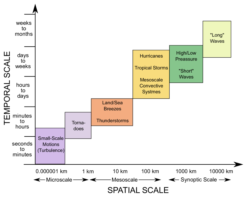
Figure 1: Typical meteorological graph about time and length scales in the atmosphere. Own reproduction.

In the remainder of this Letter, we will first introduce the idea of a power law dependence of the error growth rate on the error magnitude and show that this leads to a strictly finite prediction horizon. We then introduce a class of dynamical systems which shows exactly this behavior, and present as a specific example a hierarchy of coupled Lorenz96-1 models where numerical simulations validate a power law divergence of the error growth rate. Finally, we re-interprete data from the study by Harlim et al.[13] and show that what they observed is a power law divergence of error growth rates, which becomes evident in our new presentation of their data.

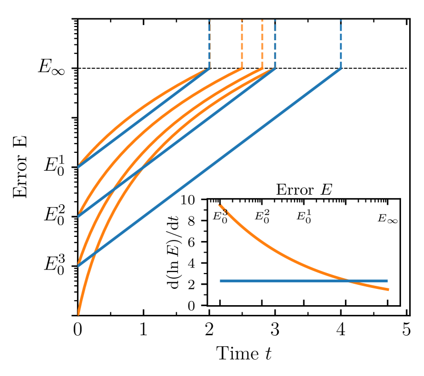
Figure 2: Exponential error growth in chaotic systems in blue, power law error growth according to (3), prediction horizons indicated by vertical dashed lines. The inset shows the divergence of scale dependent growth rate $\lambda(E)$ as opposed to a standard Lyapunov exponent.

2 Power law divergence of scale dependent error growth

Let us assume that the dynamics exhibits a scale dependent error growth rate $\lambda(E):=\frac{\mathrm{d}\ln(E(t))}{\mathrm{d}t}|_{E(t)=E}$ where the rate of growth is a power law with an exponent $-\beta$ and some coefficient $a>0$ and where $E$ is the magnitude of a perturbation:

$$\frac{\mathrm{d}\ln(E)}{\mathrm{d}t}=\frac{\dot{E}}{E}=aE^{-\beta}.$$ (2)

Integration by separation of variables leads to a power law growth of errors.

$$E(t)=(E_{0}^{\beta}+a\beta t)^{1/\beta}.$$ (3)

As for classical exponential error growth, Equation (3) becomes invalid for very large times $t$ when the error saturates at a value $E_{\infty}$ related to the finite extent of the attractor. What is strikingly different here is the diverging error growth rate for small $E_{0}$ and small $t$. The linear increment $\Delta t$ we gain in prediction time every time we cut the error $E_{0}$ into half becomes smaller and smaller (see Figure 2). The overall prediction time converges to a finite value - a maximum prediction horizon $t_{\rm{max}}$. If the tolerable maximal error is denoted by $E_{\rm tol}$ then $t_{\rm max}$ is given by

$$t_{\rm pred}=\frac{E_{\rm tol}^{\beta}-E_{0}^{\beta}}{a\beta}\rightarrow t_{\rm{max}}=\frac{E_{\rm tol}^{\beta}}{a\beta}<\infty\mbox{ for }{E_{0}\to 0}$$ (4)

This is a new and severe form of chaos, which we propose to exist in systems with an infinite dimensional phase space. While we assume that under certain conditions this will be exhibited by PDEs which intrinsically form cascades such as the Richardson cascade in turbulence, we present here a paradigmatic model class which is based on coupled low-dimensional systems with a hierarchy of scales imposed by our choice of parameters.

Given a chaotic $N$-dimensional dynamical system in terms of an ODE, $\dot{\vec{x}}=\vec{F}(\vec{x})$, we introduce a hierarchical coupling by defining a family of spatial scaling factors $\alpha_{i}$ decreasing in $i$ and of temporal scaling factors $\tau_{i}$ increasing in $i$. Here $i$ denotes the level of the hierarchy, where $i=1$ is the top level and $i=L$ the lowest. For the $i$-th level, we replace $\vec{x}$ by $\vec{x}_{i}/\alpha_{i}$ and $t$ by $\tau_{i}t$ and we obtain the equations of motion

$$\dot{\vec{x}}_{i}=\tau_{i}[\alpha_{i}\vec{F}(\vec{x}_{i}/\alpha_{i})+\vec{C}(\vec{x}_{i+1},\vec{x}_{i-1})]\;,$$ (5)

for $i=1,\ldots,L$. Here, $\vec{C}(\vec{a},\vec{b})$ denotes a weak coupling term which in the simplest case might be linear, $\vec{C}(\vec{a},\vec{b})=\vec{a}+\vec{b}$ (also weak global coupling is thinkable). For a finite number of levels $L$, the non-existing coupling inputs $\vec{x}_{0}$ and $\vec{x}_{L+1}$ are set to zero, and the system then has $NL$ degrees of freedom. Since coupling is weak and if the dynamics $\vec{F}$ generates just one positive Lyapunov exponent $\lambda$, the hierarchical system has $L$ positive Lyapunov exponents which are approximately $\lambda_{i}\approx\lambda\tau_{i}$. We chose the families of $\alpha_{i}$ and $\tau_{i}$ being monotonous in such a way that the top level hierarchy is slow but that the spatial extent of its attractor and the error saturation value $E_{\infty}$ is large, and that the lowest level is the fastest and its phase space range is the smallest.

For infinitesimal errors, the error growth is governed by the maximum Lyapunov exponent $\lambda\tau_{L}$ of the fastest time scale, but this error growth saturates at the scale $\alpha_{L}$ which is small. Then the second largest Lyapunov exponent of the second lowest level takes over, till also this error growth saturates at a scale of $\alpha_{L-1}$, and so on. This way we generate a scale dependent error growth rate, where the properties of this scale dependence are tunable.

One specific tuning which generates the proposed power-law-divergence of the error growth rate is to chose both families of scaling factors in a geometric way, i.e., $\tau_{i}=c^{i}$, and $\alpha_{i}=d^{i}$. As we will demonstrate by the help of the specific example below, the resulting power $\beta$ of the scaling of $\lambda(E)\propto E^{-\beta}$ is then $\beta=\ln c/\ln d$. Clearly, for finite $L$ this divergence is cut-off by a maximum rate of $\lambda(E)\leq\lambda\tau_{L}$.

3 Multi-hierarchical model L96-H

We specify now the general model class by choosing the model L96-1 introduced in Lorenz (1996)[14] for the dynamics $\vec{F}(\vec{x})$. Its governing equations, using the notation of [14], read

$$\dot{x}_{n}=x_{n-1}\left(x_{n+1}-x_{n-2}\right)-x_{n}+F$$ (6)

with $n=1\dots N$ , $x_{n}$ cyclic permutable with $x_{n\pm N}=x_{n}$, and $F$ a constant driving force. For $N>6$ and $F>8$ all instances behave chaotically with increasing positive largest Lyapunov exponent for increasing $N$ and $F$. Its equations of motion for some inner level $i$ read

$$\dot{x}_{n,i} = \tau_{i}\Big{[}\frac{1}{\alpha_{i}}x_{n-1,i}\left(x_{n+1,i}-x_{n-2,i}\right)-x_{n,i}$$ (8)

$$+\alpha_{i}F_{i}+x_{n,i+1}+\frac{\alpha_{i+1}}{\alpha_{i-1}}x_{n,i-1}\Big{]}\;.$$

The system is $LN$ dimensional and the state space can be divided into $L$ subspaces of dimension $N$ for each level of the hierarchy. We denote the state vector by $\vec{X}=\{\vec{x}_{1},\dots,\vec{x}_{L}\}$ with $\vec{x}_{i}\in{\rm I\!R}^{N}$. The coupling is bidirectional with upwards coupling from lower to higher level $x_{n,i+1}$ and with downwards coupling $\frac{\alpha_{i+1}}{\alpha_{i-1}}x_{n,i-1}$. The pre-factor $\frac{\alpha_{i+1}}{\alpha_{i-1}}$ is chosen such that the downwards coupling has the same magnitude as the upwards coupling. In the lowest level the undefined scale $\alpha_{L+1}$ is chosen as continuation of the sequence of $\alpha_{i}$. The term $\alpha_{i}F_{i}+x_{n,i+1}+\frac{\alpha_{i+1}}{\alpha_{i-1}}x_{n,i-1}$ can be considered as time dependent driving force $F_{i}(t)$. It is important to make sure that $F_{i}(t)>\alpha_{i}\cdot 8$ for all times to ensure that each level is chaotic.

In the following, we will present numerical results of this system for the parameters $N=7$, $F=15$ for which the single level dynamics (without coupling) is chaotic with a maximal Lyapunov exponent of $\lambda\approx 2.66$ and an error saturation value $E_{\infty}\approx 22$.

We define the error $E(t)$ as the ensemble average of the Euclidean distance between a reference trajectory and an initially randomly perturbed error trajectory with perturbation strength $E_{0}$. Thereby we distinguish between the error of the total system $\vec{X}$ denoted $E_{\rm{tot}}(t)$ and the error $E_{i}(t)$ regarding only the subspace of one single level $\vec{x}_{i}$. The scale dependent error growth rate is defined as the time derivative of the logarithm of the error $\frac{\mathrm{d}\ln E}{\mathrm{d}t}$ as a function of the error magnitude $E(t)$ at time $t$. Indeed, one can also study the propagation of the error from level to level by initial perturbations in selected levels only, which leads to interesting transient behaviors but eventually converges to error growth as for a global perturbation.

We study a hierarchy of $L=5$ levels with the scale factors $\tau_{i}=2^{i-5}$ and $\alpha_{i}=10^{5-i}$. The random initial perturbation has magnitude $E_{0}=10^{-2}$ while the saturation value is at $E_{\infty,1}\approx E_{\infty}\alpha_{1}=22\cdot 10^{4}$. In Figure 3 the error growth is shown on a double logarithmic plot. Both, the total error $E_{\rm tot}(t)$ (blue) and the error growth of the levels $E_{i}(t)$ show power-law behavior, where the errors measured in the sub-spaces of a certain level have additional features to be discussed elsewhere. For the resulting power law error growth, the interplay of level-$i$-Lyapunov exponents $\lambda\tau_{i}$ and of their saturation scales $E_{\infty,i}\approx E_{\infty}\alpha_{i}$ is crucial. The inset shows the numerically determined error growth rates as a function of error magnitude. The parameters $\tau_{i}$ and $\alpha_{i}$ are chosen such that the error growth rate decreases by a factor of $1/2$ every time the error becomes larger by a factor of $10$. This proportionality is shown by the bold dashed line with $\mathrm{d}(\ln E)/\mathrm{d}t\propto E^{-\ln(2)/\ln(10)}$.

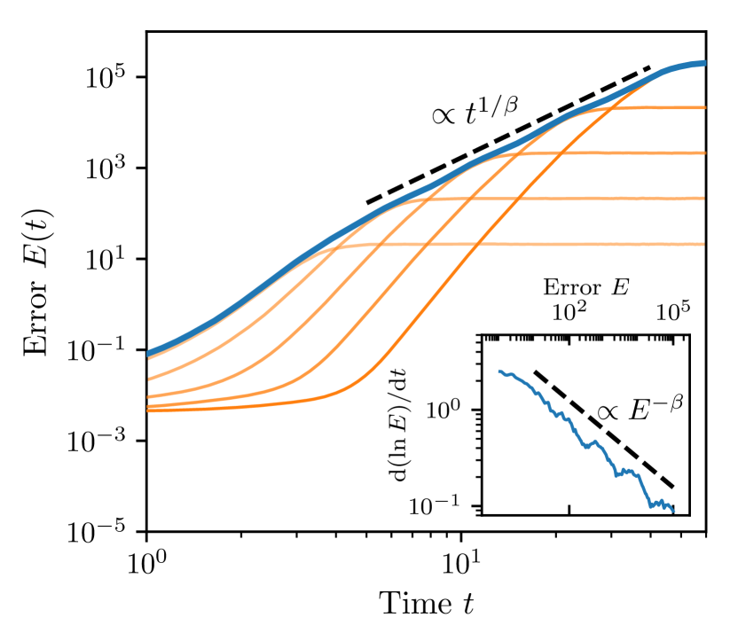
Figure 3: Power-law error growth of the model L96-H on a double-logarithmic plot

4 Re-analysis of the Harlim et al. results

We have presented evidence that a power law divergence of error growth rates can be realized by a dynamical system with properties which resemble the observed coupling of time and length scales in the atmosphere. Here, we want to strengthen this concept by a study of a numerical weather forecast system. Actually, since the authors of this article do neither have the skills nor the resources to do a study on real weather forecasts, we use published results to support our ideas. Harlim et al.[13] have performed extensive numerical experiments with the Global Forecast System of the National Center for Environmental Prediction (NCEP -GFS), focusing with their studies on mid-latitudes wind prediction (vorticity). We recall here some details from their original publication, for more see[13]. They applied perturbations to reference trajectories and measured numerically the rate of divergence of such two trajectories as a function of their Euclidian distance in phase space. The results are depicted in Figure 1 of [13] as a scatter plot of error growth rate versus error magnitude. We used the free software “WebPlotDigitizer” [15] to obtain the coordinates of an essential sub-set of the dots in this diagram. These data, in the same representation as the original figure (inset), and on a doubly logarithmic scale are shown in Figure 4. Evidently, the error growth rate in this system can be well described by a power law with divergence for small errors Equation (2), and the estimated power $\beta$ is about $0.63$. There is hence considerable evidence that a real weather forecast model does suffer not only from scale dependent error growth, but that this is indeed governed by a power law with a maximum prediction horizon of 15-16 days, when we use Equation (4), insert $E_{\infty}=1$ (which is the saturation value in the normalization of [13]), a time unit of days, and $a=0.1$ and $\beta=0.63$ as obtained by our fit.

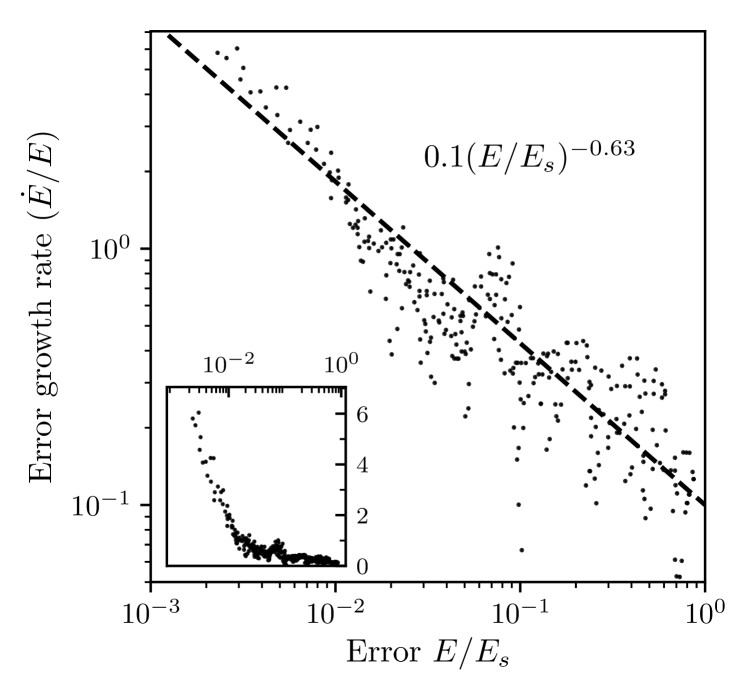
Figure 4: The dots are taken from Figure 1 of Harlim et al.[13] and denote error growth rate in units of 1/day as a function of error magnitude for a numerical weather model. The line is a power law fit with power $\beta=0.63$. The inset shows the scanned data in a representation as in the original publication and verifies that our recording of the plotted data is reasonable.

5 Conclusions

Based on the idea of scale dependent error growth, which is motivated by meteorological evidence, we proposed the possibility of deterministic dynamical systems with a strict prediction horizon, which is given if the error growth rate diverges for small error magnitudes like a power law. We proposed a class of chaotic dynamical systems which exhibit such a behavior and illustrated this by a model system. The system models the spatial and temporal hierarchies present in atmospheric dynamics. We then re-analyzed data produced in [13] in terms of a power law divergence of error growth rates and found thereby that indeed in this weather forecast system, this power law divergence is present and that the maximum forecast range is limited to 15 days. We find it plausible that the same holds for other weather forecast systems, as already also stated for the European IFS[11]. The dynamical origin of this phenomenon lies in the linkage of spatial and temporal scales of this multi-scale phenomenon, where the smallest scales are the fastest.

References

- [1] Lorenz, E. N. (1963), Deterministic Nonperiodic Flow. J. Atmos. Sci. 20, 130.
- [2] Bauer, P., Thorpe, A., and Brunet, G. (2015). The quiet revolution of numerical weather prediction. Nature, 525(7567):47–55.
- [3] Ott, E. (2002). Chaos in Dynamical Systems. Cambridge University Press, 2nd edition.
- [4] Thompson, P. D. (1957). Uncertainty of Initial State as a Factor in the Predictability of Large Scale Atmospheric Flow Patterns. Tellus, 9(3):275–295.
- [5] Robinson, G. D. (1967). Some current projects for global meteorological observation and experiment. Q. J. R. Meteorol. Soc., 93(398):409–418.
- [6] Lorenz, E. N. (1969). The predictability of a flow which possesses many scales of motion. Tellus, 21:289–307.
- [7] Palmer, T. N., Döring, A., and Seregin, G. (2014). The real butterfly effect. Nonlinearity, 27(9).
- [8] Robinson, G. D. (1971). The predictability of a dissipative flow. Q. J. R. Meteorol. Soc., 97(413):300–312.
- [9] Leith, C. E. and Kraichnan, R. H. (1972). Predictability of Turbulent Flows. J. Atmos. Sci. 29 1041-1058.
- [10] Smagorinsky, J. (1969). Problems and promises extended range forecasting. Bull. Amer. Meteor. Soc., 50, 286–312.
- [11] Zhang, F., Qiang Sun, Y., Magnusson, L., Buizza, R., Lin, S.-J., Chen, J.-H., and Emanuel, K. (2019). What is the Predictability Limit of Midlatitude Weather? J. Atmos. Sci. doi: 10.1175/JAS-D-18-0269.1, in press.
- [12] Cencini, M. and Vulpiani, A. (2013). Finite size Lyapunov exponent: review on applications. J. Phys. A Math. Theor. 46(25):254019.
- [13] Harlim, J., Oczkowski, M., Yorke, J. A., Kalnay, E., and Hunt, B. R. (2005). Convex error growth patterns in a global weather model. Phys. Rev. Lett. 94, 228501.
- [14] Lorenz, E. N. (1996). Predictability – a problem partly solved. Predict. Weather Clim., pages 40–58.
- [15] WebPlotDigitizer Version 4.1 by Ankit Rohatgi, https://automeris.io/WebPlotDigitizer/