Particle Filter on Episode

Abstract

Differently from animals, robots can record its experience correctly for long time. We propose a novel algorithm that runs a particle filter on the time sequence of the experience. It can be applied to some teach-and-replay tasks. In a task, the trainer controls a robot, and the robot records its sensor readings and its actions. We name the sequence of the record an episode, which is derived from the episodic memory of animals. After that, the robot executes the particle filter so as to find a similar situation with the current one from the episode. If the robot chooses the action taken in the similar situation, it can replay the taught behavior. We name this algorithm the particle filter on episode (PFoE). The robot with PFoE shows not only a simple replay of a behavior but also recovery motion from skids and interruption. In this paper, we evaluate the properties of PFoE with a small mobile robot.

1 Introduction

Animals are receiving vast amount of information from their sense organs. Their brains may discard most of the information. However, they can convert a part of information into abstract knowledge. For example, researchers in neuroscience have found that some special types of neurons in a mammal compose maps of its environment [1, 2]. With the maps, mammals recognize where they are and where/how they should go. Even if they forget their past experiences, they can recognize places.

Mobile robots can also build and utilize maps of their environments with SLAM (Simultaneous localization and mapping) software[3]. In the process of a SLAM algorithm, a robot periodically receives a set of data from its sensors and its odometry or dead reckoning module. A SLAM algorithm converts this data sequence into a map. Though the sequential order gives important information to the SLAM algorithm, it is not recorded in the map.

Though there are similarities in the process of map building between animals and robots, a difference also exists. When a robot is recording a data sequence on the main memory of its computer, it never disappears until it is explicitly erased. When a person must memorize a long sequence of numbers correctly, he/she feels difficulty. On the other hand, robots can memorize a long data sequence if they have a large amount of DRAM, and can recall each data in the sequence correctly. Since a raw data sequence for a map contains more information than the map, there is a possibility that we can devise some decision making algorithms which directly use the sequence. To make a robot use such an algorithm in real time, we must solve the problem of calculation amount.

This paper reports that a simple particle filter applied to data on a time sequence has the ability of real-time decision making in the real world. This particle filter is named PFoE (particle filter on episode). Particle filters[4] have been successfully applied to real-time mobile robot localization as the name Monte Carlo localization (MCL)[5, 6]. MCLs are mainly applied in the state space of a robot, while PFoE is applied in the time axis. This paper shows some experimental results. The robot performs some teach-and-replay tasks with PFoE in the experiments. The tasks are simple and could also be handled by some deep neural network (DNN) approaches[7, 8]. However, unlike DNN, the particle filter generates motions of robots without any learning phase for function approximation. Moreover, unlike MCL, it never estimates state variables directly. This phenomenon has never been reported.

The structure of this paper is as follows. Section 2 describes related works. Section 3 gives the problem that PFoE solves. The algorithm is explained and examined in Sections 4 and 5 respectively. We conclude this paper in Section 6.

A part of the work in this paper derives from our conference paper [9], and Japanese conference papers [10, 11]. We use a generalized definition in the explanation of the method in this paper. Moreover, we add experiments for quantitative evaluations and discussion.

2 Related works

PFoE uses a particle filter, which is frequently used for self-localization of a robot [5, 6]. Particle filters for self-localization are known by the name of Monte Carlo localization (MCL). MCL concentrates its particles in some areas where its owner may exist. The particles are candidates of the actual poses of the robot. Since the calculation amount is in proportion to the number of particles, MCL can work in a large environment. PFoE also utilizes this advantage of particle filters. Though MCL needs a map of the environment in which a robot works, PFoE does not need it.

Teach-and-replay for mobile robots is an attractive subject [12, 13, 14, 15, 16]. Its goal is to make a mobile robot autonomously behave as controlled by a trainer previously. To make a mobile robot work in an environment with a conventional way, we must prepare the map of the environment with a SLAM (simultaneous localization and mapping) method [3, 17], implement a self-localization method such as MCL, and write navigation codes. If teach-and-replay becomes possible, these labor hours disappear.

Teach-and-replay for mobile robots and autonomous vehicles has been studied in the context of vision-based feedback control [12, 13, 14, 16]. In a teaching phase, a sequence of images are recorded. After that, some feature points are extracted from the images. In the replay phase, the feature points in each image are compared to those of the current image. A robot is controlled as the both sets of feature points are matched. In [15], a two-dimensional laser scanner is used instead of a camera. In this study, a scan matching method is used for feedback control.

In [14, 16], teach-and-replay methods were applied to long-distance navigation tasks. These methods divide a path obtained in a teaching phase into segments. In a replay phase, the vehicle tries to move from the start to the end of each segment by comparison of images. Especially in [16], Nitsche et al. have used MCL for measuring the rate of progress in a segment. This MCL does not use a global coordinate system, and estimates the rate of progress with dead reckoning. There are some points of similarity between this method in [16] and PFoE. However, PFoE does not use the concept of self-localization, or absolute/relative positions in a coordinate system. Though PFoE has never been applied to long distance navigation, PFoE can generate various behaviors of a robot in spite of its primitive structure. Moreover, PFoE does not need any explicit implementation of feedback control. This is a major difference between PFoE and the others.

PFoE handles a decision making problem as a hidden Markov model (HMM). In an HMM [18, 19], a finite number of states are defined, and state transitions of the system are hidden from an observer. Instead, the observer can receive a sequence of observations. Many algorithms on HMMs have been proposed for pattern recognition problems[19]. Techniques for HMMs are also utilized for motion recognition or motion generation of robots [20, 21]. They have focused their attention on recognition of sequences of motion. To make a robot move in the real world with the recognition result, feedback control as researched in the above teach-and-replay methods will be required. In other research fields, combinations of an HMM model and a particle filter can be seen [22, 23]. Their purposes are also recognition.

In [24], we have proposed another PFoE as an algorithm for reinforcement learning. Possibly we will unify this PFoE and the PFoE in this paper in future. However, they are different with each other in this stage.

Differently from recurrent neural network (RNN)[25], long short-term memory (LSTM)[26, 27], and other neural network architectures, PFoE does not use back-propagation learning. This is a difference between PFoE and them. More than that, it is important that a particle filter has an ability of teach-and-replay. Though it can only be applied to some easy tasks at this time, the phenomena caused by PFoE should be reported as a new discovery. Combinations of the idea of PFoE and some state-of-art methods will be interesting topics in future.

3 Problem Definition

We want to teach an autonomous robot various motions or simple tasks without changing the software and its parameters on the robot. The robot is taught its motion by a trainer through a wireless game controller. Here we formulate this problem.

3.1 The system

We assume a time-invariant system with a state space $\mathcal{X}$. In the system, a sequence of discrete time steps are defined as $\mathcal{T}=\{\dots,t-2,t-1,t,t+1,t+2\dots\}$. The state of the system at $t$ is then written as $x_{t}\in\mathcal{X}$. There is a robot in this system. This robot does not have the knowledge on the system except that it is time-invariant.

The robot can periodically observe its surroundings and take an action. Here we define the symbols $z_{t}$ and $a_{t}$ which denote an observation at $t$ and an action at $t$ respectively. Though an observation and an action are abstract words, they correspond to a set of sensor readings and a move of actuators in the experiment section. Just after the robot finishes the action $a_{t}$, it obtains the observation $z_{t}$. After that, it chooses the next action $a_{t+1}$. We define an event $e_{t}=(a_{t},z_{t})$.

A state and an observation are related with a probability $P(z_{t}|x_{t})$. The state transition rule also exists as a probability $P(x_{t}|x_{t-1},a_{t})$. However, the robot does not know them.

3.2 Teaching (obtaining an episode)

To teach behavior, a trainer controls the robot from an initial state. We define the start time as $t=0$. During the control, the robot records an event $e_{t}=(a_{t},z_{t})$ at every time step. The recording starts from $t=1$. This procedure is named a teaching phase.

After a teaching phase, the robot memorizes the following sequence:

$$\mathcal{E}_{\text{teach}} =\{a_{1},z_{1},a_{2},z_{2},a_{3},\dots,a_{T},z_{T}\}$$

$$=\{e_{t}|t=1,2,\dots,T\},$$

where $T$ is the time step at which the trainer stopped teaching. We name the sequence $\mathcal{E}_{\text{teach}}$ the episode of this teaching phase.

Though the robot cannot observe the sequence of states in the teaching, we write it as

$$\mathcal{X}_{\text{teach}}=\{x_{0},x_{1},x_{2},\dots,x_{T}\}$$ (1)

for explanation. Since we use a mobile robot in the experiments, a sequence of states is called a path in this paper.

3.3 Replay (decision making with the episode)

After the teaching phase, we want to make the robot replay $\mathcal{X}_{\text{teach}}$ based on $\mathcal{E}_{\text{teach}}$. This phase is named a replay phase.

In this phase, the robot obtains an event $e_{\tau}=(a_{\tau},z_{\tau})$ at every time step. $\tau$ denotes the latest time step, at which the robot must decide and take an action $a_{\tau+1}$.

Our target is not a simple replay in which the robot has only to trace the sequence of actions $a_{1},a_{2},\dots,a_{T}$. The robot must give feedback to its motion so as to deal with motion errors and sensor noises. Then, it must resume the replay just after a sudden interruption.

Though it is merely a matter of form, we evaluate a path on a replay $\mathcal{X}_{\text{replay}}$ with

$$J(\mathcal{X}_{\text{teach}},\mathcal{X}_{\text{replay}})\in\Re.$$ (2)

Though we will use various evaluation criteria in Section 5, they can be defined with this form. From the standpoint of the optimal control theory, an evaluation function should be defined before the implementation of a controller. However, it is not fixed since the robot is given various tasks. Therefore, the optimality of PFoE cannot be discussed in this paper. Instead, we will show the versatility of PFoE.

4 Particle Filter on Episode

We propose a particle filter which searches similar events to the current event $e_{\tau}$ from an episode $\mathcal{E}_{\text{teach}}$. The robot takes an action by reference to the action(s) at the similar events. As a result, the robot replays the path on the teaching.

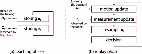
We show the flow of PFoE in Figure 1. The figure (a) illustrates the teaching phase explained in Section 3.2. Actions and observations are just recorded in this phase. In (b), the procedures motion update and measurement update are related to Section 4.2.1 and 4.2.2 respectively. Resampling are briefly written in the end of Section 4.2.2. Decision making is described in Section 4.3.

Figure 1: Flow charts of PFoE

4.1 A probability distribution on the episode and its approximation

We define a probability distribution $Bel_{\tau}$ which gives the probability

$$Bel_{\tau}(x_{t}) =P(x_{\tau}\approx x_{t}|e_{\tau},Bel_{\tau-1})$$

$$=P(x_{\tau}\approx x_{t}|a_{\tau},z_{\tau},Bel_{\tau-1})\quad(\forall x_{t}\in\mathcal{X}_{\text{teach}}).$$ (3)

$Bel_{\tau}$ is called the belief on PFoE. This belief quantifies the similarity between the current state $x_{\tau}$ and each $x_{t}\in\mathcal{X}_{\text{teach}}$. We should pay attention to that $x_{\tau}$ never becomes equal to $\forall x_{t}\in\mathcal{X}$ if $\mathcal{X}$ is not discrete. Therefore, we did not write as $x_{\tau}=x_{t}$ but wrote as $x_{\tau}\approx x_{t}$. The similarity is indirectly defined by a likelihood function, which is explained later. In Equation (3), we have assumed that the belief should be calculated from the previous belief and the latest event. $Bel_{\tau}$ fulfills $\sum_{t=0}^{T}Bel_{\tau}(x_{t})=1$.

In PFoE, the belief $Bel_{\tau}$ is approximated by a particle filter which has $N$ particles. Each of the particles is represented as

$$\xi_{\tau}^{(i)}=(t_{\tau}^{(i)},w_{\tau}^{(i)})\quad(i=1,2,\dots,N).$$ (4)

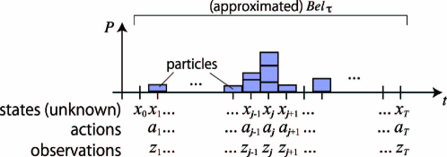
In this formulation, $i$ is the index of each particle, $t_{\tau}^{(i)}$ points a time step in the training phase, and $w_{\tau}^{(i)}$ denotes the weight of the particle. With these particles, each probability $Bel_{\tau}(x_{t})$ is represented by

$$Bel_{\tau}(x_{t}) =\sum_{i=1}^{N}\delta(x_{t}=x_{t_{\tau}^{(i)}})w_{\tau}^{(i)}\qquad(\delta(\text{true})=1\text{ and }\delta(\text{false})=0)\color[rgb]{0,0,1}.\color[rgb]{0,0,0}$$ (5)

Figure 2 explains this approximation. The height of each particle represents its weight. Equation (5) means that the value $Bel_{\tau}(x_{t})$ is equal to the summation of the heights of the particles at $x_{t}$. In this figure, $x_{j}$ is considered as the most similar state to $x_{\tau}$ because $x_{j}$ has the largest sum of the weights among the states.

Figure 2: Belief $Bel_{\tau}$ represented by the particles

4.2 State estimation on the episode

PFoE updates $Bel_{\tau-1}$ after an event $e_{\tau}=(a_{\tau},z_{\tau})$. At first, the action $a_{\tau}$ is reflected in the belief. This step makes the particles diffuse on the time axis, and the belief becomes uncertain. Next, $z_{\tau}$ is used for reducing the uncertainty.

4.2.1 Update with the latest action

After $a_{\tau}$, PFoE shifts the belief $Bel_{\tau-1}$ based on $P(x_{\tau}|x_{\tau-1},a_{\tau})$. This calculation conforms to the following equation of Markov chain:

$$\widehat{Bel}_{\tau}(x_{t}) =P(x_{\tau}\approx x_{t}|a_{\tau},Bel_{\tau-1})$$

$$=\sum_{t^{\prime}=0}^{T}P(x_{\tau}\approx x_{t}|x_{\tau-1}\approx x_{t^{\prime}},a_{\tau})Bel_{\tau-1}(x_{t^{\prime}}),$$ (6)

where $\widehat{Bel}_{\tau}$ is the belief in which $z_{\tau}$ is not reflected. Since this equation does not take care that the time axis ends at $T$, it should be cared on the implementation. The more important problem is that the state transition probability $P(x_{\tau}=x_{t}|x_{\tau-1}=x_{t^{\prime}},a_{\tau})$ is unknown. However, when the interval between $\tau-1$ and $\tau$ is short, the state transitions will not be largely different from those of the teaching phase. On the other hand, this optimistic assumption should be partially denied. We prepare a constant number $\Delta$ as the rate of denial of the assumption.

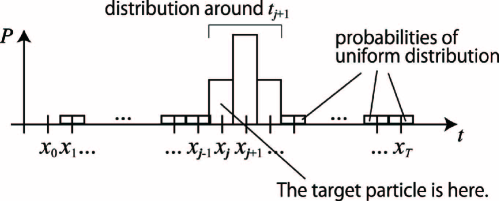
Based on this idea, PFoE updates the belief from $Bel_{\tau-1}$ to $\widehat{Bel}_{\tau}$ by a simple way. This procedure changes the time step $t_{\tau-1}^{(i)}$ of each particle to $\hat{t}_{\tau}^{(i)}$, which is chosen as

$$\hat{t}_{\tau}^{(i)} \sim P(t|t_{\tau-1}^{(i)})=(1-\Delta)\cdot P_{\alpha}(t|t_{\tau-1}^{(i)})+\Delta\cdot P_{\beta}(t).$$ (7)

$$\bullet\ P_{\alpha}:\text{a distribution around }t_{\tau-1}^{(i)}+1$$

$$\bullet\ P_{\beta}:\text{the uniform distribution on the time axis from $t=1$ to $t=T$}$$

The first term of the right side of Equation (7) means that the particle at the time step $t_{\tau-1}^{(i)}$ will go to a time step near $t_{\tau-1}^{(i)}+1$ with the probability $1-\Delta$. With the probability $\Delta$, the time step is chosen randomly with $P_{\beta}$. Figure 3 illustrates an example of the probability distribution $P(t|t_{\tau-1}^{(i)})$ when the particle before the update is at $t=t_{j}$.

Incidentally, when some particles go over the time axis, they are replaced randomly on the time axis. Then, any particle is not placed at $t=0$ because the procedure in Section 4.2.2 cannot handle particles at $t=0$.

Figure 3: The probability distribution for the update of a particle

4.2.2 Update with the latest observation

After an observation of $z_{t}$, the belief should be updated by the following Bayes’ theorem:

$$Bel_{\tau}(x_{t})=P(x_{t}|z_{\tau},\widehat{Bel}_{\tau}) =\dfrac{P(z_{\tau}|x_{t})\widehat{Bel}_{\tau}(x_{t})}{\sum_{t^{\prime}=1}^{T}P(z_{\tau}|x_{t^{\prime}})\widehat{Bel}_{\tau}(x_{t^{\prime}})}$$

$$=\mu P(z_{\tau}|x_{t})\widehat{Bel}_{\tau}(x_{t}),$$

where $\mu$ is the normalizing constant[3]. With a likelihood function $L(x_{t}|z_{\tau})\propto P(z_{\tau}|x_{t})$, the above equation is represented as

$$Bel_{\tau}(x_{t}) =\mu L(x_{t}|z_{\tau})\widehat{Bel}_{\tau}(x_{t}).$$

When we use MCL, a likelihood function is given as a previous knowledge of the robot. However, there is a problem that $L(x_{t}|z_{\tau})$ is unknown in the problem defined in Section 3.

Instead, PFoE uses $L(z_{t}|z_{\tau})$ as the likelihood function. Since $z_{t}$ is the only information directly related to $x_{t}$ in the episode, this substitution is the only way to measure the relation between $z_{\tau}$ and $x_{t}$.

With this likelihood function, PFoE updates the weight of each particle from $w_{\tau-1}^{(i)}$ to $w_{\tau}^{(i)}$ by the following substitution:

$$w_{\tau}^{(i)}=w_{\tau-1}^{(i)}L(z_{t_{\tau}^{(i)}}|z_{\tau}).$$ (8)

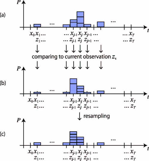
This procedure generates the set of particles ${\xi^{\prime}}_{\tau}^{(i)}=(\hat{t}_{\tau}^{(i)},w_{\tau}^{(i)})\ (i=1,2,\dots,N)$, which represents $Bel_{\tau}$. From Figure 4(a) to (b), this procedure is illustrated.

After that, a resampling method creates another set of particles $\xi_{\tau}^{(i)}=(t_{\tau}^{(i)},1/N)\ (i=1,2,\dots,N)$ that also represents $Bel_{\tau}$. This procedure eliminates the bias of weights. It is also used in MCL for the same purpose. From Figure 4(b) to (c), this procedure is illustrated. We assume that PFoE uses the systematic sampling, which is usually chosen for MCL[3].

Figure 4: Update after the observation

4.3 Decision making

The next action $a_{\tau+1}$ is chosen based on $Bel_{\tau}$. Formally, this decision making is written as

$$a_{\tau+1}=\Pi(Bel_{\tau}),$$

where $\Pi$ stands for a mapping from a probability distribution to an action. It is called a decision making policy.

While we cannot fix the one and only implementation of $\Pi$, we can formulate some types of policy. In Section 5, we try the following two policies.

The simplest one can be given as

$$\Pi_{\text{mode}}(Bel_{\tau}) =a_{\hat{t}+1},$$ (9)

$$\text{where}\quad\hat{t} =\mathop{\rm argmax}\limits_{t}Bel_{\tau}(x_{t}).$$

Here, $x_{\hat{t}}$ is the mode of $Bel_{\tau}$. Therefore, this policy chooses the action of the next time step of the mode. We name this policy the mode policy.

We can also define a policy that uses a mean value of actions weighted by $Bel_{\tau}$ if the calculation is possible. This policy is represented as

$$\Pi_{\text{mean}}(Bel_{\tau}) =\sum_{t=0}^{T-1}Bel_{\tau}(x_{t})a_{t+1}.$$ (10)

When the action can be represented as a vector with some real numbers, this calculation is possible. This policy is named the mean policy.

5 Experiments

We investigate what PFoE can and cannot do with a mobile robot. Other methods will not be tried in the experiments for comparison since they will need additional experimental assumptions or sensors as explained in Section 2. We will verify that PFoE can work on a small mobile robot with a small computer and cheap sensors, and observe various phenomena caused by PFoE.

We have never changed any parameter of PFoE for all of the experiments in this section. The setting of the parameters is described in Section 5.1.

5.1 Implementation to an actual robot

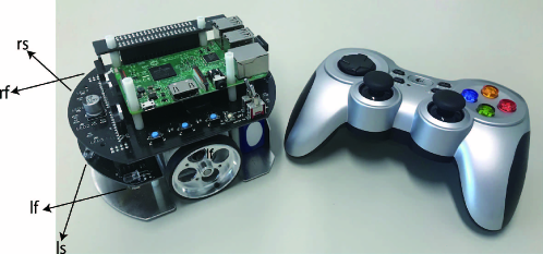
We implement PFoE to Raspberry Pi Mouse[28], which is a parallel two-wheel vehicle type mobile robot. As shown in Figure 5, it has two step motors and four range sensor units. As the name suggests, it has a Raspberry Pi 3, which is a well-known single-board computer. Since we will use this robot as a fully autonomous one in the later experiments, all software programs for this robot including PFoE work on the Raspberry Pi 3. The game controller in the figure is used for training.

5.1.1 Definition of action and observation

We define an action as

$$\boldsymbol{a}=(v_{\text{linear}},v_{\text{angular}}),$$

where $v_{\text{linear}}$ and $v_{\text{angular}}$ are the linear and angular velocities of the robot respectively. This definition is straightforwardly derived from the interface of a base ROS package (https://github.com/ryuichiueda/raspimouse_ros_2) of this robot. This package translates them to the revolution speeds of the step motors. Since an action becomes a vector in this case, we use the bold type $\boldsymbol{a}$ for representing an action.

In a training phase, we can give $v_{\text{linear}}=0.2$[m/s] to the robot with the up key. When the up key is not pushed, $v_{\text{linear}}=0$. We can also give $v_{\text{angular}}=\pm\pi/2$[rad/s] to it with the right and left keys. When these keys are not pushed, $v_{\text{angular}}=0$. These linear and angular velocities can be given simultaneously. Since the tires of Raspberry Pi Mouse are very slippy, these velocities easily decrease by the condition of the floor.

An observation is defined as

$$\boldsymbol{z}=(z_{\text{lf}},z_{\text{ls}},z_{\text{rs}},z_{\text{rf}}),$$

where the four variables denote the raw values from the “left forward (lf),” “left side (ls),” “right side (rs),” and “right forward (rf)” sensors respectively. Their names are written in Figure 5. Since $\boldsymbol{z}$ is a vector, we use the bold type.

Figure 5: Robot (left) and game controller (right)

Figure 6: Relation between distances from the wall and sensor values

The range sensors are not as accurate as recent laser range finders. Each of them is composed of an infrared LED and a light sensor. The LED emits infrared light, and the light sensor measures the intensity of the reflected light. Since the direction of each sensor can be changed by a touch, the measured values change easily. They are also exposed to vibration when the robot is running. Moreover, the values are also affected by the color and material of the wall that reflects the light.

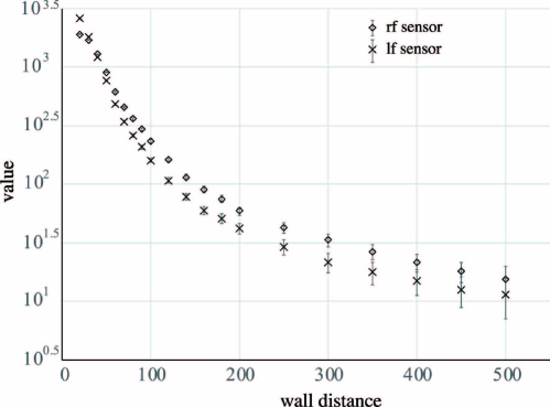
Figure 6 shows the character of the sensors in the case where the robot is not moving. In the experiment for this data, we placed the robot at right angle to the wall in the corridor used in Figures 7 and 16 later. We changed the distance, and recorded the values of the lf and rf sensors every second for one hour with each distance. Vertical bars on the data points represent the standard deviations. As shown in the difference between the data of lf and rf, each sensor has its own bias even on the logarithmic scale.

5.1.2 Update procedures

After an action, each particle goes to the next time step with $30$[%], moves two steps forward with $30$[%], does not move with a probability of $30$[%], or is replaced randomly with $10$[%]. It means that $\Delta=0.1$, and that $P_{\alpha}$ in Equation (7) is the following uniform distribution:

$$P_{\alpha}(t|t_{\tau-1}^{(i)})=\begin{cases}1/3&(t=t_{\tau-1}^{(i)},t_{\tau-1}^{(i)}+1,t_{\tau-1}^{(i)}+2)\\ 0&(\text{otherwise})\end{cases}.$$ (11)

After an observation, the weight of each particle is changed with the following likelihood function:

$$L(\boldsymbol{z}_{t}|\boldsymbol{z}_{\tau})=\prod_{j=\text{lf,ls,rs,rf}}\dfrac{1}{|\log_{10}z_{jt}-\log_{10}z_{j\tau}|+1},$$ (12)

where $z_{jt}$ denotes the value of the $j$ sensor in $\boldsymbol{z}_{t}$. The value of this function becomes one when $\boldsymbol{z}_{t}=\boldsymbol{z}_{\tau}$. We choose this function so as not to make PFoE sensitive to the difference when the sensor values are large.

5.1.3 Other conditions

Events of the first and last five seconds are removed from the episode since silent events at preparation and finishing may be contained in these parts. The number of particles $N$ is fixed to $1000$. At the start of a replay trial, particles are randomly placed on the episode $\mathcal{E}_{\text{teach}}$. The cycle of time steps is fixed to $100$[ms]. The trainer in all of the experiments is the first author, except that it is the third author in the person following task. They are accustomed to controlling the robot.

5.2 Counting task

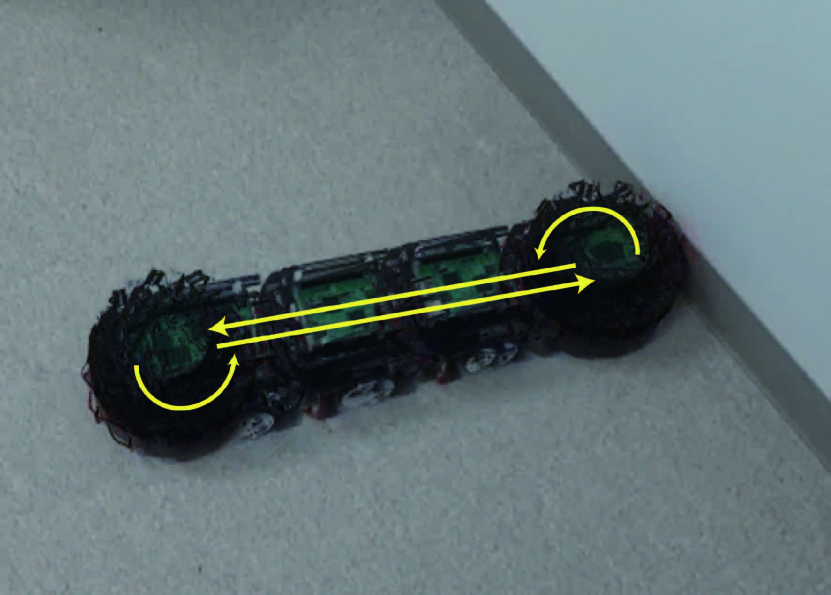
At first, we make the robot count a number by its motion. In this task, the trainer places $500$[mm] apart from the wall. After that, he makes the robot bump the wall, swing its nose right and left several times, and step back $500$[mm] as illustrated in Figure 7(a). The trainer repeats this motion several cycles without a break. The angle of the swinging is about $45$[deg] toward the wall. We define the number of counts $n$, which is incremented when the robot’s nose starts leaving the wall by a left or right swing. This number is taught to the robot by the control of the trainer. Figure 7(b) and (c) show the cases where $n=1$ and $n=2$ respectively.

Figure 7: The counting task

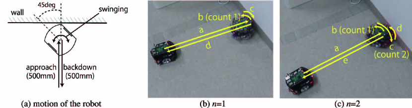
We use this task for evaluating how long PFoE can trace an episode. If the robot miscounts in a cycle of replay, we consider this cycle as a failure. The larger the value of $n$, the longer the robot must replay the sequence of actions. Miscounts will occur when the mode of the particles leaps from an event to another due to the random resampling, sensor noises, or motion errors. Moreover, the robot must approach the wall and back down from it with a right angle. If the robot crossly approaches the wall, the trace of the episode falls into disorder. Obviously, the robot must decide its action in consideration of the temporal context of this task. It is impossible by a decision making method that decides the robot’s action only based on the latest sensor values.

5.2.1 Result

For evaluation, we had five sets of teach-and-replay for each number of $n$ ($n=1,2,\dots,8$). In one set, we had three cycles of the motion at teaching, and conducted ten cycles of replay just after that. Each cycle at the replay is called a trial hereafter. In each trial, we recorded whether the robot counted $n$ correctly or not.

Table 5.2.1 shows the number of successful trials of each set. This result was obtained with the mode policy. The mean policy did not work well. It sometimes stopped the robot because Equation (10) offset the forward motion and the backward motion.

As shown in this table, the robot could count $n$ without any mistake when $n\leq 2$. Even when $n=6$, it kept a success rate of more than 80[%]. When $n=7$ and $8$, the percentages were at around half. In this table, we can see that the success counts of three sets are peculiarly smaller than the others on the same rows. It seems that their teaching phases had some problems. Practically, since we can discard bad teaching results, we can expect larger success rates than those on the table.

Numbers of success trials on the counting task (mode policy)   $n$ set 1 set 2 set 3 set 4 set 5 all 50 replays $1$ 10 10 10 10 10 50 (100[%]) $2$ 10 10 10 10 10 50 (100[%]) $3$ 6 9 9 10 10 44 (88[%]) $4$ 9 9 10 10 10 48 (96[%]) $5$ 9 9 4 9 10 41 (82[%]) $6$ 8 10 9 7 7 41 (82[%]) $7$ 7 6 0 8 5 26 (52[%]) $8$ 3 6 5 3 7 24 (48[%])  

Figure 8: Poses of the robot at the teaching and replay phases

5.2.2 Behavior of particles

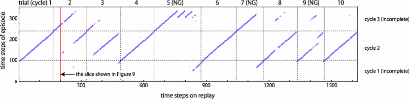
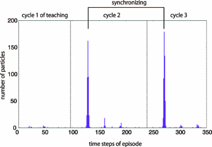
To investigate the behavior of particles in this task, we had another set of the teach-and-replay with $n=6$. Figure 9 shows where the mode of the belief existed at each time step of the trials. The horizontal and vertical coordinate values of each point are time steps at replay and teaching respectively. The horizontal and vertical dashed lines in the figure delimit the cycles (trials). We noticed that this episode contained only one complete cycle due to the five second cut of beginning and end. The first and last cycles in this episode started and ended in the process of counting respectively. However, the robot could count the number successfully seven times in the ten trials. Figure 10 shows the distribution of particles at the 200th step of the replay. We can find that this distribution is multi-modal. It has several modes. The highest one is the mode shown in Figure 9.

As shown in Figure 9, the mode of particles leaped frequently. This leap occurs when the highest mode in the distribution switches after an observation. When the highest mode changes to another at the same phase of another cycle, a mistake does not occur. However, a miscount happens when the phases are different. At the $200$th step, for example, the mode existed in the third cycle of the episode. After that, the mode arrived at the end of episode and disappeared. Instead, the second mode in the second cycle became the main mode. Since these modes pointed the same phase of counting, the robot could count correctly in this replay cycle. In the fifth, seventh, and ninth cycles, miscounts occurred since the phases were not synchronized. For this problem, loop closing techniques used in SLAM [29] will be helpful. Then we need to improve our implementation so as not to cut the start and end of an episode. Though these approaches are attractive as future works, they may complicate the software. What is important here is that particles in PFoE can trace several points in an episode, and change the mode with a degree of accuracy.

Figure 9: Transition of mode ($n=6$)

Figure 10: Distribution of particles at a time step on replay

5.3 Choice task

We have another task in which the robot must choose a path in a micromouse maze. The environment is shown in Figure 11. In the teaching phase, the trainer makes the robot run from the start point (“S” in the figure) to the end of a target pocket three times. The target pocket is chosen from A, B, or C in the figure, and fixed in the three runs. When the robot reaches the end in the first and second runs, the trainer replaces the robot at the start point. Recording of the episode is not stopped during the replacements.

Figure 11: The environment for the choice task

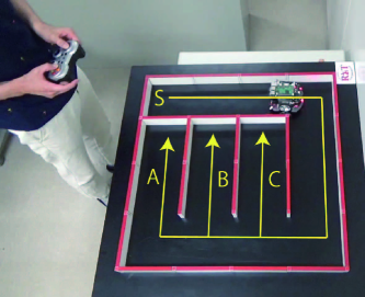
In the replay phase, we have ten trials. In a trial, the robot is placed at the start without any signal. It must start running autonomously, and must reach the target pocket. When the center of the robot enters in the target pocket, the trial is regarded as a successful one. The robot does not need to reach the end deeply. When the robot stops several seconds without entering a pocket, the trainer replaces the robot at the start point, and this trial is regarded as a did not finish (DNF) trial.

We had three sets of teach-and-replay with the mean policy for each target pocket (nine sets in total). Then, we had other nine sets with the mode policy. Incidentally, the trainer had two hours of practice before this experiment.

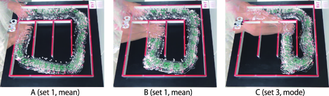
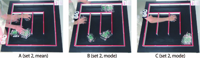
The results are illustrated in Table 5.3. The success rates were $83$[%] and $61$[%] with the mean policy and the mode one respectively. This percentages will change by the skill or concentration of the trainer. In five sets with the mean policy, the robot did not mistake. Even with the mode policy, the success rates were equal to or more than $90$[%] in five sets. If the trainer can teach appropriately, the robot can distinguish the three kinds of paths. Figures 13 shows composite pictures of the robot in three successful sets respectively. The paths in each set of ten trials are drawn in each of them.

Figure 13 shows composite pictures of three unsuccessful sets. In these pictures, the final poses of the ten trials are drawn respectively. As shown in the second and third pictures, the mode policy frequently made the robot stop before reaching a pocket. The robot mistook as it finished a trial frequently when it faced the wall. That is the reason why DNF trials of the mode policy were more than those of the mean one. The robot with the mean policy also stopped in the same situation. However, it escaped the situation in many cases since the mean policy did not make the robot stop completely. With a slight motion, the robot got a change of sensor readings, and it made a trigger of the escape.

Incidentally, the robot could stop its wheels when the trainer picked up it, and start just after the replacement in every trial. Though the explicit start and end of trials were never recorded in the episodes, the robot distinguished whether it was in the maze or not based on the sensor readings.

Numbers of success trials on the choice task   set pocket mean mode   set 1 A 10/10     9/10 B 10/10     3/10 C     7/10     9/10 set 2 A     4/10     5/10 B 10/10     0/10 C     9/10     1/10 set 3 A 10/10     9/10 B 10/10     9/10 C     5/10 10/10 success trials 75/90 (83[%]) 55/90 (61[%]) DNF trials 7/90   ( 8[%]) 31/90 (34[%]) mischoice trials 8/90   ( 9[%]) 4/90   ( 4[%]) success trials in finished trials 75/83 (90[%]) 55/59 (93[%])  

Figure 12: Paths of the robot on the best experimental set for each pocket

Figure 13: Final poses of the robot on the worst experimental set for each pocket

5.4 Wall following task

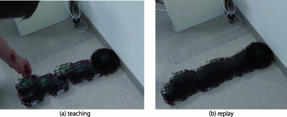
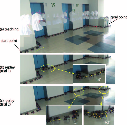
Next, we make the robot follow the indented wall of an elevator hall. In a training phase, the trainer controls the robot as shown in Figure 15(a) only once. At a replay trial, we make the robot run from the start point to the goal point behind the rightmost dustbox. If the robot can reach the goal point, it is regarded as a success. Though we do not evaluate the success rate in this task, we aim for five consecutive successful trials without failure after a training phase. We do not give the robot any start signal at the beginning of each trial.

In this task, the robot only has to react the latest sensor readings. Instead, the robot must maintain the follow of the wall after a skid or a bump against the wall by its feedback motion. A problem is that the ability of PFoE to trace an episode has the possibility to inhibit the feedback motion.

Figure 14: Wall following task

Figure 15: Change of mode in the wall following task

We spent about two hours to the experiment. In the two hours, successful sets of teach-and-replay increased progressively due to the habituation of the trainer. Though some troubles which were not related to PFoE occurred in replay trials, we obtained one successful teach-and-replay set with the mean policy and two successful sets with the mode policy.

Figures 15(b) and (c) show the first and second replay trials with the episode obtained by the teaching in Figure 15(a). The mode policy was used for these trials. In these trials and the other three trials, the robot successfully followed the wall with its feedback motion. In many cases where the robot largely got away from the wall, it returned to the wall with behaviors shown in the enlarged images (b)’ and (c)’. Though these kinds of large recovery motion were not directly taught in the teaching, they were generated by PFoE. Figure 15(c)” is an extreme case, where the robot ran around in circles at the corner after it lost the wall (to be more exact, the dustbox). Such a motion was never taught to the robot.

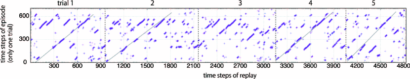
Figure 15 shows the transition of the mode in the five trials. As shown in this diagram, the mode leaped frequently. If these leaps were prohibited, the robot would not take appropriate feedback. Though tracing of an episode is the main feature of PFoE, it can also discard a trace quickly.

On the other hand, we can find in Figure 15 that the mode was synchronizing with the sequence of the training. Particles of the modes on the gray diagonal lines have the information of the progress of this task. Though this information was not required for this task, we could found that PFoE partially sustained the trace of the episode.

5.5 Wall following and corridor crossing task

Lastly, we prepare a task that requires not only the feedback motion as shown in the wall following but also the trace of an episode. In the task named the wall following and corridor crossing task, the robot runs on a rectangle path as shown in Figure 16(a). During the intervals B and D shown in (a), the trainer controls the robot as it follows the wall. The trainer makes the robot turn 90[deg] in the ends of B and D, and makes it go straight in A and C.

Figure 16: Teaching and replay phases on the wall following and corridor crossing task

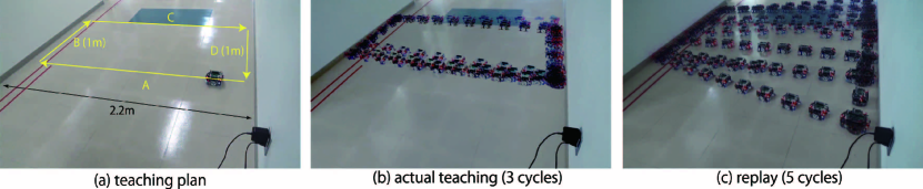
After three cycles of a teaching phase, we made the robot replay five cycles (trials) continuously. All of the cycles in the teaching and replay are shown in Figures 16(b) and (c) respectively. As shown in (c), the paths at the replay were cluttered since the lengths of the wall following varied.

In Table 5.5, we wrote out the amounts of time consumed in the intervals B and D. We can find that four values in the row of replay are smaller than the minimum value in the row of teaching.

Time for intervals B and D   $n$ cycle 1 cycle 2 cycle 3 cycle 4 cycle 5 interval B D B D B D B D B D avg. (std. dev.) teaching 5.0 5.3 4.3 4.8 3.4 5.3 - - - - 4.7 (0.7) replay 1.2 4.5 4.4 5.3 5.7 3.2 2.1 3.0 4.2 3.7 3.7 (1.6)  

Figure 17: Transition of mode in the set of the wall following and corridor crossing task

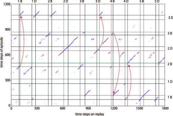
We can understand the reason with Figure 17. In the intervals that were finished in short time, the modes leaped too early to beginning time steps of the intervals A or C. Since leaps frequently occur in the wall following part as mentioned in Section 5.4, the information of the time is easily lost. This is a major problem of the current version of PFoE. Though we have already tried an idea for this problem in [30], it has never been matured.

Though we also tried the mean policy for this task, the motion of the robot was inaccurate. In this case, the angles when the robot left from a wall did not become 90[deg].

5.6 Discussion about the choice of policies

Equation (10) of the mean policy prevents the robot from moving when some clusters of particles suggest contradictory actions. This effect was shown in the counting task. Moreover, Equation (10) obscures the amount of displacement even when the robot must move accurately. This effect was observed in the wall following and corridor crossing task.

On the other hand, the mode policy is not the only option. It just utilizes one of feature amounts of $Bel$. We should consider a combination of several statistics of $Bel$ in future works.

5.7 Other behaviors

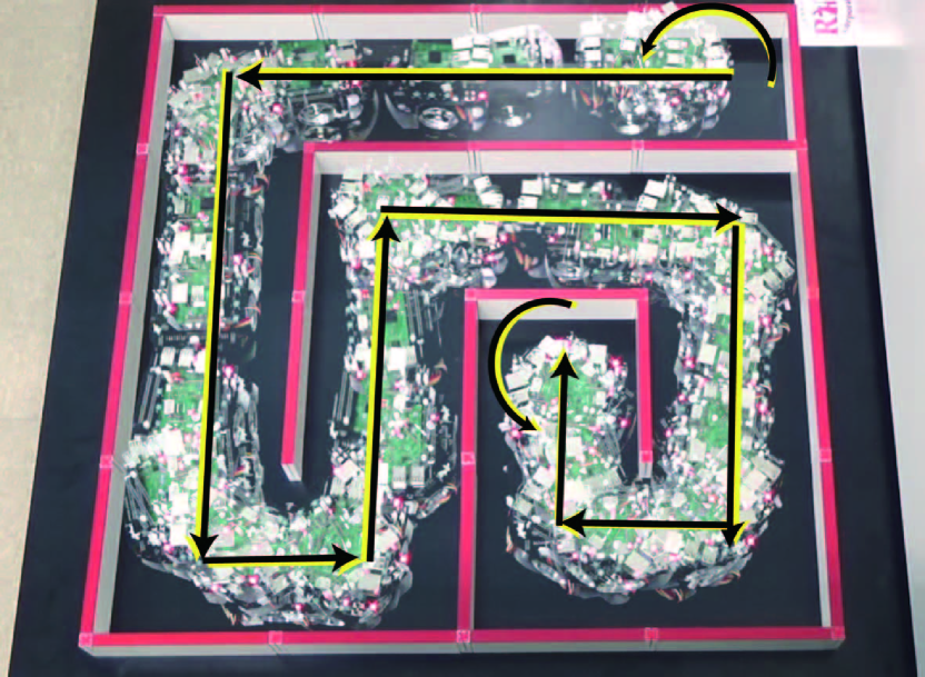
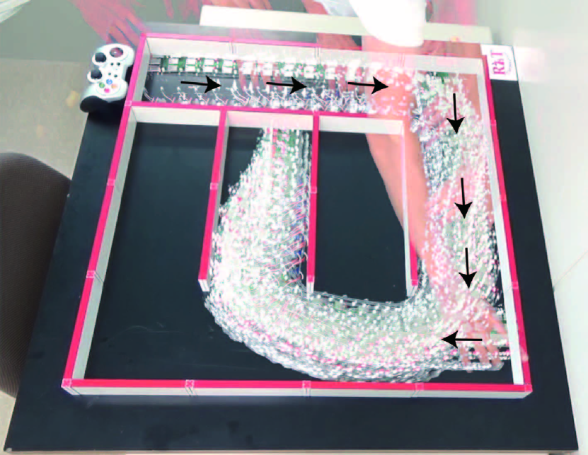
We have generated various behaviors of the robot with the same parameter set. Figure 19 illustrates a cycle of replay in a micromouse maze. Since the robot easily skids and hits the walls, feedback control is important for stable run. When we took the movie for this figure, we had three cycles of teaching and ten minute replay. We used the mode policy. In the replay, the robot ran the path without stopping, while the robot took irregular 180-degree turns twice. Though PFoE should be able to make the robot trace mazes which have several intersections, the success rates in the choice task are not enough for multiple choices. A high level teaching skill or a patchwork technique of episodes will be required.

In Figure 19, the robot had a 180-turn both at the front of wall and the farthest point from the wall. This is a modified version of the counting task.

Figure 18: Running in a maze

Figure 19: A behavior in front of the wall

Figure 20: Choice task from different start points

Figure 21: A part of trial of person following

In Figure 21, paths of seven consecutive replay trials are illustrated at the choice task. These paths start from the different points, which are indicated by arrows in the figure. The training was done with the same start point in Figure 11. The target pocket was B. The mean policy was used.

As shown in the figure, the robot repeatedly chose the target pocket in spite of the difference of the start points. This case was the best one, and the robot sometimes made mistakes in other sets. However, this result suggests that PFoE does not require strict start points in some tasks. In [9], we can see another case where PFoE shows the robustness. In this case, the counting task was interrupted and restarted from a different point. However, the robot could get the rhythm immediately.

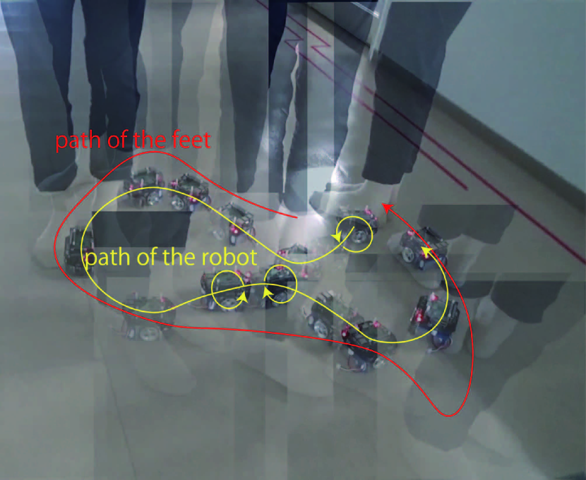
Figure 21 shows the paths of a person and the robot in a person following task. In the teaching phase, the trainer rotated the robot as a search behavior when the target person was far from it (farther than about 30[cm]). When the target was near, the trainer made the robot follow him. We spent 80[s] for this training. Figure 21 is a composite picture of some scenes in 80[s] replay. The three hoops on the path of the robot mean the points where the robot took the search behavior. Though this figure does not tell it, the robot could appropriately choose the search behavior and the following behavior as it taught in the teaching phase.

5.8 Calculation amount

Finally, we measured the time consumption of PFoE on Raspberry Pi 3, which has a ARM Cortex-A53 1.2 GHz processor. Though this processor has four CPU cores, our implementation of PFoE runs on a single thread.

In a measurement, $m$ cycles of the counting task were trained. Then we logged the time consumption of each procedure in PFoE at the replay phase. Since we did not use a real-time kernel, large delays unrelated to the calculation occurred once in about ten time steps. We chose five consecutive time steps that did not contain the delay from the log, and took the averages of them. We tried $m=3,10,20$.

The results are shown in Table 5.8. Since the time complexity of every procedure in PFoE is $O(N)$, the time length of each procedure never extends by the increase of the length of the episode.

Time for each step of PFoE on Raspberry Pi 3 (unit: millisecond)   lengths of teaching 3 cycles 10 cycles 20 cycles update with an action 1.51 1.56 1.55 update with an observation 4.47 4.52 4.46 resampling 1.27 1.29 1.28 decision making (mode policy) 0.72 0.72 0.72 total 7.97 8.09 8.01  

There is a problem that the calculation amount of the update with an observation is in proportion to the number of the sensors. As shown in the table, the update with an observation is the heaviest procedure in PFoE since four sensor values have to be reflected to the weight of every particle one by one. Since MCL and online SLAM have exactly the same problem, we will be able to utilize the techniques for MCL and online SLAM [3] for it. However, it is still a future work.

6 Conclusion

We have proposed PFoE, which uses a particle filter not for mobile robot localization but for making a robot recall and replay memory of the past. Our implementation of PFoE is extremely simple. The concepts of states, positions, and distances are not used in it. However, it can work on the actual robot.

In the experiments, we have obtained the following knowledge:

• PFoE can make the robot replay behaviors that have temporal contexts as shown in the counting task though the length is still limited.

• PFoE can also deal with tasks that have spatial contexts as shown in the wall following task.

• PFoE can also make the robot replay behaviors that have not only spatial contexts but temporal contexts as shown in the counting task. In the counting task, the robot could count six successfully more than 80[%] of the time.

• PFoE with the parameters mentioned in Section 5.1 generates various motions of the robot.

• A step of PFoE which uses 1,000 particles can be calculated in 8[ms] on a 1.2 GHz ARM processor regardless of the length of the episode.

We have also confirmed some problems of PFoE through the experiments. Since the mean and mode policies are only feature amounts of $Bel$, there is a room for improvement of policies. Moreover, for applying PFoE to long term tasks, unnecessary leaps of the mode should be reduced.

References

- [1] J. O’keefe and J. Dostrovsky, “The hippocampus as a spatial map. Preliminary evidence from unit activity in the freely-moving rat,” Brain Research, vol. 34, no. 1, pp. 171–175, 1971.
- [2] G. Buzsáki and E. I. Moser, “Memory, navigation and theta rhythm in the hippocampal-entorhinal system,” Nature Neuroscience, vol. 16, no. 2, pp. 130–138, 2013.
- [3] S. Thrun, W. Burgard, and D. Fox, Probabilistic ROBOTICS. MIT Press, 2005.
- [4] N. J. Gordon, D. J. Salmond, and A. F. M. Smith, “Novel approach to nonlinear/non-Gaussian Bayesian state estimation,” IEE Proceedings-F, vol. 140, no. 2, pp. 107–113, 1993.
- [5] F. Dellaert, D. Fox, W. Burgard, and S. Thrun, “Monte Carlo Localization for Mobile Robots,” in Proc. of IEEE International Conference on Robotics and Automation (ICRA99), 1999, pp. 1322–1328.
- [6] D. Fox, “Adapting the Sample Size in Particle Filters Through KLD-Sampling,” International Journal of Robotics Research, vol. 22, no. 12, pp. 985–1003, 2003.
- [7] N. Hirose, R. Tajima, and K. Sukigawa, “MPC policy learning using DNN for human following control without collision,” Advanced Robotics, vol. 32, no. 3, pp. 148–159, 2018.
- [8] H. A. Pierson and M. S. Gashler, “Deep learning in robotics: a review of recent research,” Advanced Robotics, vol. 31, no. 16, pp. 821–835, 2017.
- [9] R. Ueda, M. Kato, A. Saito, and R. Okazaki, “Teach-and-replay of mobile robot with particle filter on episode,” in Proc. of IEEE International Conference on Robotics and Automation, Brisbane, Australia, 2018, pp. 3475–3481.
- [10] R. Ueda, “Particle filter on episode for teaching,” in Proc. of the 35th Annual Conference of the Robotics Society of Japan, Kawagoe, Japan, 2017 (in Japanese).
- [11] M. Kato, R. Ueda, and R. Okazaki, “An application of Particle Filter on Episode for Teaching — Replay of Path Selection and Motion Control of a Mobile Robot by Humans,” in Proc. of the 35th Annual Conference of the Robotics Society of Japan, Kawagoe, Japan, 2017 (in Japanese).
- [12] Z. Chen and S. T. Birchfield, “Qualitative Vision-Based Mobile Robot Navigation,” in Proceedings of the 2006 IEEE International Conference on Robotics and Automation, 2006, pp. 2686–2692.
- [13] A. Cherubini, M. Colafrancesco, G. Oriolo, L. Freda, and F. Chaumette, “Comparing appearance-based controllers for nonholonomic navigation from a visual memory,” in ICRA 2009 Workshop on safe navigation in open and dynamic environments: application to autonomous vehicles, Kobe, Japan, 2009.
- [14] T. Krajník, J. Faigl, V. Vonśek, K. Košnar, and M. K. L. Přeučil, “Simple yet stable bearing‐only navigation,” Journal of Field Robotics, vol. 27, no. 5, pp. 511–533, 2010.
- [15] C. Sprunk, G. D. Tipaldi, A. Cherubini, and W. Burgard, “Lidar-based teach-and-repeat of mobile robot trajectories,” in In Proc. of IEEE/RSJ International Conference on Intelligent Robots and Systems (IROS), 2013.
- [16] M. Nitsche, T. Pire, T. Krajník, M. Kulich, and M. Mejail, “Monte Carlo Localization for Teach-and-Repeat Feature-Based Navigation,” in Advances in 15th Annual Conference on Autonomous Robotics Systems, 2014, pp. 13–24.
- [17] M. Montemerlo, FastSLAM: A Factored Solution to the Simultaneous Localization and Mapping Problem With Unknown Data Association. Carnegie Mellon University: Doctor Thesis, 2003.
- [18] L. E. Baum and T. Petrie, “Statistical Inference for Probabilistic Functions of Finite State Markov Chains,” The Annals of Mathematical Statistics, vol. 37, no. 6, pp. 1554–1563, 1966.
- [19] C. M. Bishop, Pattern Recognition and Machine Learning. Springer, 2006.
- [20] K. Sugiura, N. Iwahashi, H. Kashioka, and S. Nakamura, “Learning, Generation and Recognition of Motions by Reference-Point-Dependent Probabilistic Models,” Advanced Robotics, vol. 25, no. 6-7, pp. 825–848, 2011.
- [21] F. Dawood and C. K. Loo, “Humanoid Behaviour Learning through Visuomotor Association by Self-Imitation,” in 2014 Joint 7th International Conference on Soft Computing and Intelligent Systems (SCIS) and 15th International Symposium on Advanced Intelligent Systems (ISIS), 2014, pp. 922–929.
- [22] R. Baxter, N. M. Robertson, and D. Lane, “Probabilistic behaviour signatures: Feature-based behaviour recognition in data-scarce domains,” in Proc. of 13th International Conference on Information Fusion (Fusion 2010), 2010, pp. 1–8.
- [23] A. Mushtaq and C. Hui-Lee, “An integrated approach to feature compensation combining particle filters and hidden Markov models for robust speech recognition,” in Proc. of IEEE International Conference on Acoustics, Speech and Signal Processing (ICASSP), 2012, pp. 4757–4760.
- [24] R. Ueda, K. Mizuta, H. Yamakawa, and H. Okada, “Particle Filter on Episode for Learning Decision Making Rule,” in Proc. of The 14th International Conference on Intelligent Autonomous Systems (IAS-14), Shanghai, China, 2016.
- [25] H. Mayer, F. Gomez, D. Wierstra, I. Nagy, A. Knoll, and J. Schmidhuber, “A System for Robotic Heart Surgery that Learns to Tie Knots Using Recurrent Neural Networks,” in Proceedings of IEEE/RSJ International Conference on Intelligent Robots and Systems, 2006, pp. 543–548.
- [26] S. Hochreiter and J. Schmidhuber, “Long Short-Term Memory,” Neural Computation, vol. 9, no. 8, pp. 1735–1780, 1997.
- [27] A. Graves and J. Schmidhuber, “Framewise phoneme classification with bidirectional LSTM networks,” in Proceedings of IEEE International Joint Conference on Neural Networks, 2005, pp. 2047–2052.
- [28] R. Ueda, Learning ROS robot programming with Raspberry Pi. Nikkei BP, 2018.
- [29] A. Kawewong, N. Tongprasit, and O. Hasegawa, “A speeded-up online incremental vision-based loop-closure detection for long-term SLAM,” Advanced Robotics, vol. 17, no. 27, pp. 1325–1336, 2013.
- [30] A. Saito and R. Ueda, “Clustering of Memory Sequence for Particle Filter on Episode,” in Proceedings of the 2018 JSME Conference on Robotics and Mechatronics, Kitakyushu, Japan, 2018 (in Japanese), pp. 1A1–C13.