Jump Processes with Deterministic and Stochastic Controls

Abstract

We consider the dynamics of a 1D system evolving according to a deterministic drift and randomly forced by two types of jumps processes, one representing an external, uncontrolled forcing and the other one a control that instantaneously resets the system according to specified protocols (either deterministic or stochastic). We develop a general theory, which includes a different formulation of the master equation using antecedent and posterior jump states, and obtain an analytical solution for steady state. The relevance of the theory is illustrated with reference to stochastic irrigation to assess probabilistically crop-failure risk, a problem of interest for environmental geophysics.

I Introduction

Control theory applied to complex systems such as networks and small out-of-equilibrium devices has received increasing attention from the physics community Bechhoefer (2005); Liu and Barabási (2016); Aurell et al. (2011). Less attention has been devoted to systems characterized by random jumps, in spite of the fact that several physical systems experience abrupt, unpredictable transitions that are aptly described as random jumps (see e.g., Belousov et al. (2016); Bartlett and Porporato (2018) and references therein). In natural processes jumps are typically external, uncontrolled events; in managed systems, however, jumps also may represent an artificial control that returns the system state to a desired range. Ideally, the control (and representative jumps) should be deterministic, but often a stochastic representation is more appropriate to account for limited and imprecise controls.

Here, for a system with deterministic drift and two jumps processes, representing a natural external process and an artificial stochastic control, we pose a master equation using the recently developed Stratonovich formalism for jump processes Bartlett and Porporato (2018) along with a novel representation for the jump currents for the control jump process. The latter is especially convenient when the initial and final states of the jump are known (i.e., the set levels for the control). We then solve the master equation for the case of steady state. This class of solutions is general to any control process description; however, the class of solutions is specific to natural processes represented by a nonhomogeneous Poisson jump process forced by inputs with an exponential distribution.

In the second part of the paper we use the developed formalism to represent the soil moisture dynamics forced by random jumps of rainfall and controlled by a state-dependent stochastic irrigation input. We consider different deterministic as well as stochastic scenarios of the irrigation control. The theory can be easily extended to multiple stochastic controls used for redundancy, the details of which will be presented elsewhere. We use the solution also to derive the associated plant water stress that determines crop failure, an important problem in geophysics and environmental engineering Porporato et al. (2015). As shown by the irrigation example, the two different but interchangeable representations of the jump process and the general class of solutions highlight a framework for managing and assessing systems forced by multiple jump processes. Such type of problems also appear in nanoscale systems, in which fluctuations are rarely small and often appear in the form of sudden jumps Muratore-Ginanneschi et al. (2013); Brandner et al. (2015). Accordingly, several problems of control at the nanoscale may be tackled with the methods presented here.

II Theory

II.1 Master Equation

We consider a system described by a scalar variable $\chi$, evolving in time both deterministically, as described by the drift function $m(\chi,t)$, and randomly, as described by two jump processes. The first one represents an uncontrolled forcing, $\varphi(\chi,t)$, and the second one a controlled forcing, $\check{\varphi}(\chi,t)$, used to reset (via a jump) the variable from an antecedent state, $\chi^{-}$, to a posterior state, $\chi^{+}$, according to a specified protocol. The corresponding Langevin-type equation is

$$\frac{d\chi}{dt}=m(\chi,t)+\varphi(\chi,t)+\check{\varphi}(\chi,t),$$ (1)

and thus the term $\varphi(\chi,t)$ is the formal time derivative of a nonhomogeneous Poisson process with arrival rate, $\lambda(\chi,t)$, and state dependent marks, $b(\chi,z)$. The corresponding master equation for the probability density function (PDF), $p_{\chi}(\chi,t)$, is

$$\partial_{t}p_{\chi}(\chi,t)=-\partial_{\chi}\left(J_{m}(\chi,t)+J_{\varphi}(\chi,t)+J_{\check{\varphi}}(\chi,t)\right).$$ (2)

The drift current is

$$J_{m}(\chi,t)=m(\chi,t)p_{\chi}(\chi,t),$$ (3)

while the current for the uncontrolled jump process is conveniently represented using transition probabilities (Van Kampen, 2007; Bartlett and Porporato, 2018), i.e.,

$$\partial_{\chi}J_{\varphi}(\chi,t)=p_{\chi}(\chi,t)\int_{-\infty}^{\infty}W(u|\chi,t)du-\int_{-\infty}^{\chi}W_{S}(\chi|u,t)p_{\chi}(u,t)du,$$ (4)

where $W(\chi|u,t)$ is the transition PDF of jumping away from any prior (antecedent) state $u$ and transitioning to the (posterior) state $\chi$, while $W(u|\chi,t)$ is the transition PDF of jumping from the antecedent state $\chi$ and transitioning to any (posterior) state $u$. Moreover, $\int_{0}^{\infty}W(u|\chi,t)du=\lambda(\chi,t)$, is the frequency of jumps, while the second transition PDF is assumed here to be specific to the Stratonovich interpretation

$$W_{S}(\chi|u,t) =\frac{\lambda(u,t)p_{z}\left(\eta(\chi)-\eta(u)\right)}{|b(\chi)|},$$ (5)

where $\eta(\chi)=\int 1/b(\chi)d\chi$, and $p_{z}(z)$ is the distribution of forcing inputs, $z$. For the latter expression (5), the state $\chi$ is an intermediate value between the states before and after the jump according to the Stratonovich interpretation (Van Kampen, 2007; Suweis et al., 2011; Bartlett and Porporato, 2018).

For the control jump process, $\check{\varphi}(\chi,t)$, a description of the current based on (4) and (5) is not convenient. In fact, it would be preferable to have a description where the initial and final set points of the control are directly specified through their respective distributions. To the best of our knowledge, a representation of this type, as presented in the next section, has not yet been explicitly developed.

II.2 Characterization by antecedent and posterior PDFs

Our goal is to express the control jump current explicitly in terms of the distributions of initial and final set points, $\check{p}_{\chi^{-}}(\chi,t)$ and $\check{p}_{\chi^{+}}(\chi,t)$, respectively. To this purpose, we start from

$$\partial_{\chi}J_{\check{\varphi}}(\chi,t)=p_{\chi}(\chi,t)\int_{-\infty}^{\infty}\check{W}(u|\chi,t)du-\int_{-\infty}^{\chi}\check{W}_{S}(\chi|u,t)p_{\chi}(u,t)du,$$ (6)

where $\check{W}(u|\chi,t)$ and $\check{W}(\chi|u,t)$ are the transition PDFs of the control process. The first transition PDF, $\check{W}(u|\chi,t)$, represents the probability rate of jumping from the state $\chi$ to any state $u$. It is therefore linked to the Poisson jump frequency, as in (4),

$$\int_{-\infty}^{+\infty}\check{W}(u|\chi,t)du=\check{\lambda}(\chi,t).$$ (7)

Following (Bartlett et al., 2015; Daly and Porporato, 2007; Bartlett and Porporato, 2018), such a non-homogeneous Poisson arrival rate is linked to the antecedent PDF, $p_{\chi^{-}}(\chi,t)$, via the average rate of jumping of the control process, $\langle\check{\lambda}(t)\rangle$, as

$$p_{\chi^{-}}(\chi,t)=\frac{\check{\lambda}(\chi,t)p_{\chi}(\chi,t)}{\langle\check{\lambda}(t)\rangle}.$$ (8)

As for the second term on the right hand side of (6), the transition PDF can be expressed as the product of the jump frequency and the PDF of the increment in $\chi$,

$$\check{W}_{S}(x|u,t)=\check{\lambda}(u,t)\check{p}_{\Delta\chi|u}(\chi|u,t),$$ (9)

where $\chi^{+}=\chi^{-}+\Delta\chi$, and thus $\check{p}_{\Delta\chi|u}(\chi|u,t)$ may be interpreted as the conditional PDF $\check{p}_{\chi|u}(\chi|u,t)$. Accordingly, the posterior PDF is defined as

$$p_{\chi^{+}}(\chi,t)=\int_{-\infty}^{+\infty}\check{p}_{\Delta\chi|u}(\chi|u,t)p_{\chi^{-}}(u,t)du.$$ (10)

Combining (8), (9), and (10), one obtains

$$\int_{-\infty}^{\chi}\check{W}_{S}(\chi|u,t)p_{\chi}(u,t)du=\langle\check{\lambda}(t)\rangle p_{\chi^{+}}(\chi,t).$$ (11)

Substituting all the above relationships in (6) gives the sought expression for the control jump current

$$\partial_{\chi}\check{J}_{\varphi}(\chi,t)=-\langle\check{\lambda}(t)\rangle\left(\check{p}_{\chi^{+}}(\chi,t)-\check{p}_{\chi^{-}}(\chi,t)\right),$$ (12)

where the first term is related to the current from jumping from any prior (antecedent) state $u$ and arriving at the (posterior) state $\chi$, while the second component is related to the current from jumping away from the prior state $\chi$ to any posterior state $u$. Because the jump is directly prescribed by this formalism, we do not need to explicitly define the underlying jump process amplitude, $b(\chi,z)$, thus avoiding interpretation issues (e.g. the Itô-Stratonovich dilemma). In summary, the master equation (2) becomes

$$\partial_{t}p_{\chi}(\chi,t)=p_{\chi}(x,t)\int_{-\infty}^{\infty}W(u|\chi,t)du-\int_{-\infty}^{\chi}W_{S}(\chi|u,t)p_{\chi}(u,t)du-\langle\check{\lambda}(t)\rangle\left(\check{p}_{\chi^{+}}(\chi,t)-\check{p}_{\chi^{-}}(\chi,t)\right).$$ (13)

II.3 General Steady State Solution

For the master equation (13) in steady state and exponential PDF of the forcing term, $p_{z}(z)=\gamma e^{-\gamma z}$, a general solution can be obtained as (see Appendix A for details)

$$p_{\chi}(\chi)=-\frac{e^{-\int\left(\frac{\gamma}{b(\chi)}+\frac{\lambda\left(\chi\right)}{m\left(\chi\right)}\right)d\chi}}{m\left(\chi\right)}\left(N^{\prime}+\langle\check{\lambda}\rangle\int h(\chi)e^{\int\left(\frac{\gamma}{b(\chi)}+\frac{\lambda\left(\chi\right)}{m\left(\chi\right)}\right)d\chi}d\chi\right),$$ (14)

where $N^{\prime}$ is a normalization constant, $b(\chi)=d\chi/dy$ (see Appendix A Eq. (43)) and

$${h}(\chi)=\frac{\gamma}{b(\chi)}\left(\check{P}_{\chi^{-}}(\chi)-\check{P}_{\chi^{+}}(\chi)\right)+\check{p}_{\chi^{-}}(\chi)-\check{p}_{\chi^{+}}(\chi).$$ (15)

Note that $\check{P}_{\chi^{-}}(\chi)=\int_{-\infty}^{\chi}\check{p}_{\chi^{-}}(u)du$, and $\check{P}_{\chi^{+}}(\chi)=\int_{-\infty}^{\chi}\check{p}_{\chi^{+}}(u)du$ are the respective cumulative distribution functions (CDFs) of the antecedent and posterior PDFs.

Introducing the potential

$$\Phi(\chi)=\int\left(\frac{\gamma}{b(\chi)}+\frac{\lambda(\chi)}{m(\chi)}+\frac{\partial_{\chi}m(\chi)}{m(\chi)}\right)d\chi=\int\left(\frac{\gamma}{b(\chi)}+\frac{\lambda(\chi)}{m(\chi)}\right)d\chi+\ln\left|m(\chi)\right|$$ (16)

the solution may be written as

$$p_{\chi}(\chi)=-e^{-\Phi(\chi)}\left(N^{\prime}+\langle\check{\lambda}\rangle\int h(\chi)e^{\Phi(\chi)}d\chi\right).$$ (17)

Note that $\langle\check{\lambda}\rangle=0$ in the absence of control processes, in which case the solution of Eq. (17) reverts to the one found in Ref.Bartlett and Porporato (2018)

In lieu of $\langle\check{\lambda}\rangle$, one may consider the crossing frequency, $\upsilon(\xi)$, at the arbitrary level $\chi=\xi$, as defined by

$$\upsilon(\xi)=|m(\xi)|p_{\chi}(\xi).$$ (18)

For Eq. (18), note that the normalization constant of $p_{\chi}(\chi)$ also is a function of the average frequency, $\langle\check{\lambda}\rangle$, i.e.,

$$N^{\prime}=\frac{\langle\check{\lambda}\rangle\int_{\chi_{\min}}^{\chi_{\max}}e^{-\Phi(\chi)}\int h(u)e^{\Phi(u)}dud\chi-1}{\int_{\chi_{\min}}^{\chi_{\max}}e^{-\Phi(\chi)}d\chi}.$$ (19)

Thus, for an assumed value of $\upsilon(\xi)$, one may solve Eq. (18) for the average frequency, $\langle\check{\lambda}\rangle$.

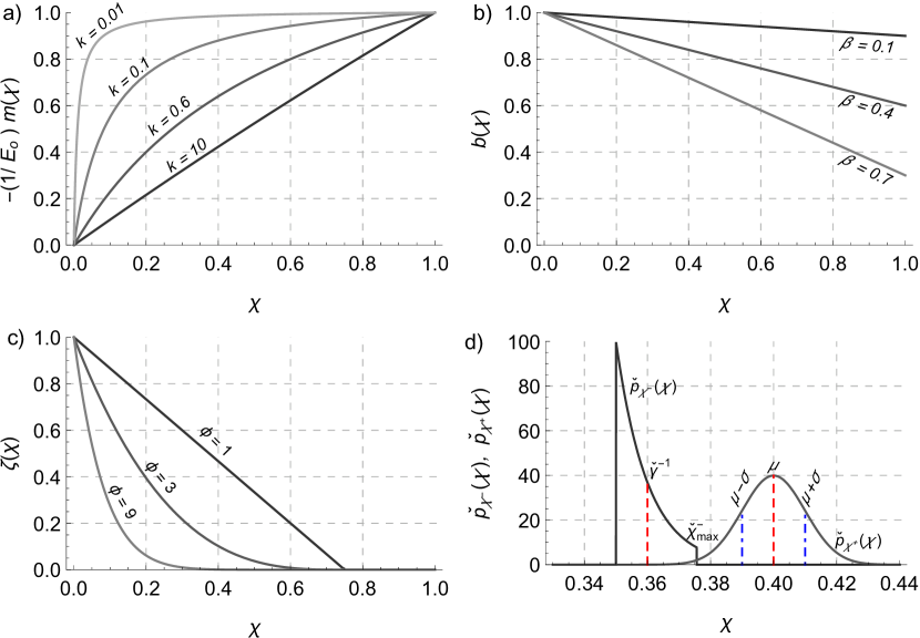
Figure 1: Examples of a) the function for evapotranspiration, $m(\chi)$, of Eq. (21) b) the function for water infiltration, $b(\chi)$, of Eq. (20), c) the function for active water stress, $\zeta(\chi)$, of Eq. (24), and d) the posterior PDF, $\check{p}_{\chi^{+}}(\chi)$, of Eq. (38), and antecedent PDF, $\check{p}_{\chi^{-}}(\chi)$, of Eq. (39), for which we have noted the $\chi$ values for $\check{\gamma}^{-1}$, $\mu$, $\mu\pm\sigma$, and the value at which the antecedent PDF is truncated, $\check{\chi}_{\max}^{-}$. Unless stated otherwise, $\chi_{\max}^{+}=1$, $\check{\chi}_{\min}=0.35$, $\check{\gamma}=100$, $\sigma=0.01$, $\mu=0.4$, $k=0.5$, $\beta=0.25$, and $f=0.9$.

III Application: Soil Moisture Dynamics with Irrigation Control

III.1 Soil Moisture and Plant Water Stress

We apply the previous theory to soil moisture dynamics, a fundamental driver of the terrestrial hydrologic cycles with feedbacks to climate and biogeochemistry (e.g., Rodríguez-Iturbe and Porporato (2004); Katul et al. (2007); Porporato et al. (2015) and references therein). The soil moisture $\chi$, defined as the relative degree of soil saturation, $0<\chi\leq 1$, jumps because of rainfall infiltration, modeled as a marked Poisson process with constant frequency $\lambda$, and rainfall marks $z$ exponentially distributed with parameter $\gamma=w_{0}/\alpha$, where $\alpha$ is the mean rainfall depth per event and $w_{0}$ is the soil water storage capacity. Following (Bartlett et al., 2015), the infiltration amount, $z\>b(\chi)$, is governed by the function

$$b(\chi)=1-\beta\chi,$$ (20)

where $\beta\chi$ represents runoff to the stream with $\chi$ interpreted in the Stratonovich sense.

During interstorm periods soil moisture decreases mostly because of plant evapotranspiration (ET), modeled as

$$m(\chi)=-E_{0}\frac{\chi(1+k)}{\chi+k},$$ (21)

where $E_{0}$ is potential evapotranspiration and the parameter $k$ adjusts $ET$ with declining soil moisture to account for different plant water use strategies (Fig. 1). Eq. (21) accounts for a variety of relationships between evapotranspiration and the soil moisture status (Mintz and Walker, 1993; Rodríguez-Iturbe and Porporato, 2004). As $k\rightarrow 0$, $m(\chi)\rightarrow E_{0}$; conversely, as $k\rightarrow\infty$, $m(\chi)$ becomes linear (see Fig. 1).

With these parameterizations, the potential function (16) is

$$\Phi(\chi)=\frac{\lambda(k\ln|\chi|+\chi)}{E_{0}(k+1)}-\frac{\gamma\ln|1-\beta\chi|}{\beta}.$$ (22)

As the soil moisture level declines, plants undergo water stress (Rodríguez-Iturbe and Porporato, 2004), modeled to occur when ET is a fraction $f$ of the potential value, $E_{0}$, at which point soil moisture is

$$\chi^{*}=\frac{fk}{f-k-1},$$ (23)

which varies with the plant water-use strategy through $k$. Below this level, $\chi^{*}$, water stress is assumed to increase as

$$\zeta(\chi)=\left(\frac{\chi^{*}-\chi}{\chi^{*}}\right)^{\phi}\quad\quad 0\leq\chi\leq\chi^{*},$$ (24)

while it is zero for $\chi>\chi^{*}$. The parameter $\phi$ accounts for the nonlinear relationship between the soil moisture deficit (from $\chi^{*}$) and water stress, and $\phi$ reflects plant water use strategies and sensitivity to drought. It is also useful to define

$$\langle\zeta^{\prime}\rangle=\frac{1}{P_{\chi}(\chi^{*})}\int_{0}^{1}\zeta\frac{\chi^{*}\zeta^{\frac{1-\phi}{\phi}}}{\phi}p_{\chi}(\chi^{*}-\chi^{*}\zeta^{\frac{1}{\phi}})d\zeta,$$ (25)

an average that only accounts for the continuous part of the PDF $p_{\zeta}(\zeta)$ and thus reflects the average over the typical duration of the stressed condition, $T_{\chi^{*}}=\frac{P_{\chi}(\chi^{*})}{|m(\chi^{*})|p_{\chi}(\chi^{*})}$. Finally, an effective stress for a growing season of duration $T_{s}$ may be defined as (Rodríguez-Iturbe and Porporato, 2004)

$$\theta=\left\{\begin{array}[]{l l}\left(\frac{\langle\zeta^{\prime}\rangle T_{\chi^{*}}}{\varpi T_{s}}\right)^{1/\sqrt{n_{\chi^{*}}}}&\quad\quad\langle\zeta^{\prime}\rangle T_{\chi^{*}}<\varpi T_{s}\\ \\ 1&\quad\quad\text{otherwise},\end{array}\right.$$ (29)

where $n_{\chi^{*}}=|m(\chi^{*})|p_{\chi}(\chi^{*})T_{s}$ is the average number of times the plant enters a stressed condition, and $\varpi$ represents an upper bound for stress prior to permanent plant damage.

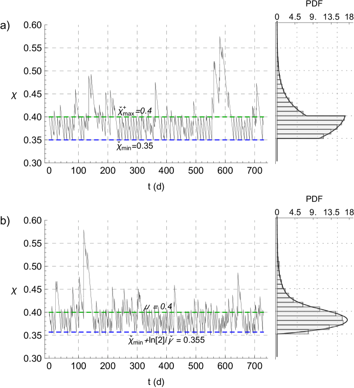
Figure 2: Examples of a) deterministic irrigation control and b) stochastic irrigation control soil moisture trajectories, simulation distribution (histogram bars), and the steady-state PDF (black lines). General parameter values are $\lambda=0.15$ d^-1, $\alpha=10$ mm, $w_{o}=450$ mm, $\gamma=w_{o}/\alpha$, $k=0.5$, $E_{0}=-4$ mm d^-1, $\beta=0.25$, $\chi_{\max}^{+}=1$, and $\check{\chi}_{\min}=0.035$. The stochastic control is based on the antecedent and posterior PDFs of Eqs. (38) and (39) for which $\sigma=0.01$, $\mu=0.4$, $\check{\gamma}=100$, and $\ln 2/\check{\gamma}$ is the median value of the antecedent PDF. In both cases, the crossing frequency is zero at $\check{\chi}_{\min}$, i.e., $\upsilon(\check{\chi}_{\min})=0$, and $\langle\check{\lambda}\rangle$ may be calculated from Eq. (18).

III.2 Irrigation

Irrigation inputs are introduced to avoid or reduce plant water stress Vico and Porporato (2011). These take place as a control in the form of instantaneous jumps, a Poisson process with rate obtainable from (8),

$$\check{\lambda}(\chi)=\langle\check{\lambda}\rangle\frac{\check{p}_{\chi^{-}}(\chi)}{p_{\chi}(\chi)}~{},$$ (30)

where $\check{p}_{\chi^{-}}(\chi)$ represents the distribution of the antecedent before irrigation initiates (see Fig. 3). The applied irrigation water, $\check{z}$, represents a forcing input that increases soil moisture by the infiltration amount given as

$$\Delta\chi=\eta^{-1}\left(\eta(u)+\check{z}\right)-u,$$ (31)

where following the Stratonovich jump interpretation of the amplitude function, $b(\chi)$, we assume that the infiltration amount decreases as the irrigation input increases based on $\eta(\chi)=\int 1/b(\chi)d\chi$. Following Eq. (31), the irrigation inputs, $\check{z}$, are greater than $\Delta\chi$ because of runoff losses implicit in the function $b(\chi)$ of Eq. (20). In turn, the applied irrigation water of Eq. (31) is part of a joint PDF for the variables governing the irrigation water amount, i.e.,

$$\check{p}_{\check{z}}(\check{z},\Delta\chi,u)=\delta\left(\check{z}-(\eta(\Delta\chi+u)-\eta(u))\right)\check{p}_{\Delta\chi|u}(\Delta\chi|u)\check{p}_{\chi^{-}}(u),$$ (32)

where the Dirac delta function, $\delta(\cdot)$, represents the PDF $\check{p}_{\check{z}|\Delta\chi u}(\check{z}|\Delta\chi,u)$, i.e., the probability density of applied irrigation, $\check{z}$, conditional on the infiltrated irrigation water, $\Delta\chi$, and the antecedent moisture state $u$. The Dirac delta function must be evaluated following the property discussed in Appendix A of (Bartlett et al., 2015). By integrating over the PDF of Eq. (32), we obtain the average depth of irrigation events,

$$\langle\check{z}\rangle=\int_{\Delta\chi_{\min}}^{\Delta\chi_{\max}}\int_{\chi_{\min}^{-}}^{\chi_{\max}^{-}}\int_{0}^{\infty}\check{z}\>\check{p}_{\check{z}}(\check{z},\Delta\chi,u)d\check{z}dud\Delta\chi.$$ (33)

Based on Eq. (33), the average volume of irrigation water required over a growing season of duration $T_{s}$ is

$$V=w_{0}\>T_{s}\langle\check{z}\rangle\langle\check{\lambda}\rangle,$$ (34)

using Eq. (33). This volume depends on the soil moisture dynamic described by the steady state PDF $p_{\chi}(\chi)$.

III.2.1 Deterministic Control

In an ideal situation of perfectly deterministic control (Vico and Porporato, 2011), irrigation initiates exactly at the intervention level $\chi=\check{\chi}_{\min}$ and brings the soil moisture to the level $\chi=\check{\chi}_{\max}^{+}$ (Fig. 2a), that is

$$\check{p}_{\chi^{-}}(\chi) =\delta(\chi-\check{\chi}_{\min})$$ (35)

$$\check{p}_{\chi^{+}}(\chi) =\delta(\chi-\check{\chi}_{\max}^{+}).$$ (36)

These and the respective CDFs (which are right continuous Heaviside step function) define a specific form of the function $h(\chi)$ of Eq. (15) The steady state PDF of soil moisture is given by Eq. (17) with substitutions for the potential of Eq. (22) and the control process average frequency, $\langle\check{\lambda}\rangle$, and setpoint function, $h(\chi)$, of Eq. (15). As a consequence of the deterministic description of the irrigation control, the solution PDF shows a sharp transition in the probability density at both the initiation level, $\check{\chi}_{\min}$, and the renewal level, $\check{\chi}_{\max}^{+}$ (Fig. 2a).

Irrigation occurs as a non-homogeneous marked Poisson process with a state dependent frequency, $\check{\lambda}(\chi)$, defined by Eq. (30) with substitutions for the steady state solution. In conjunction with $\check{\lambda}(\chi)$, the infiltrated irrigation water is distributed as

$$\check{p}_{\Delta\chi|u}(\Delta\chi|u) =\delta(\Delta\chi-(\check{\chi}_{\max}^{+}-u))$$ (37)

where irrigation events always increase soil moisture by a deterministic amount of water (per unit area) equal to $w_{0}(\check{\chi}_{\max}^{+}-\check{\chi}_{\min})$. The average depth of applied irrigation water is $\langle\check{z}\rangle=\left(\eta(\check{\chi}_{\max}^{+})-\eta(\check{\chi}_{\min})\right)$, which follows from Eqs. (32) and (33), both of which are specific to the Stratonovich interpretation of the jump transition. The overall volume of water for a growing season is given by Eq. (34).

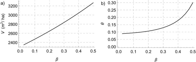
Figure 3: For deterministic irrigation controls over a growing season, $T_{s}$, and increasing $\beta$, i.e., increasing runoff, a) total volume of applied irrigation water and b) mean effective plant water stress. Parameter values are $\lambda=0.15$ d^-1, $\alpha=10$ mm, $w_{o}=450$ mm, $\gamma=w_{o}/\alpha$, $k=0.5$, $E_{0}=-4$ mm d^-1, $\beta=0.25$, $\check{\chi}_{\max}^{+}=0.4$, $\check{\chi}_{\min}=0.035$, $\varpi=0.5$, $T_{s}=$120 d, $\phi$=2, and $f=0.9$.

Unlike previous stochastic descriptions of irrigation (Vico and Porporato, 2010, 2011), here we account for runoff losses taking place below saturation (through the function $b(\chi)$ of Eq. (20)). A low value of $\beta$ could represent an overall efficient management of the agroecosystem that results in both less water losses to runoff, a smaller volume of required irrigation water (Fig. 3a), and less water stress. A larger $\beta$ is responsible for a sharp increase in plant water stress (Fig. 3b).

III.2.2 Stochastic Control

To account of imperfect control, a stochastic irrigation scheme is defined by $\check{p}_{\chi^{-}}(\chi)$ and $\check{p}_{\chi^{+}}(\chi)$, so that the control (on and off) setpoints are now random variables (Fig. 2b). Here, we represent the antecedent setpoint with an exponential PDF and the posterior setpoint with a normal PDF, both of which are truncated i.e.,

$$\check{p}_{\chi^{-}}(\chi) =\frac{\check{\gamma}e^{\check{\gamma}(\chi-\check{\chi}_{\min})}}{1-e^{-\check{\gamma}(\check{\chi}_{\max}^{-}-\check{\chi}_{\min})}}\quad\quad\quad\quad\quad\quad\quad\quad\quad\check{\chi}_{\min}\leq\chi\leq\check{\chi}_{\max}^{-}$$ (38)

$$\check{p}_{\chi^{+}}(\chi) =\frac{2\>e^{-\frac{(\chi-\mu)^{2}}{2\sigma^{2}}}}{\sqrt{2\pi}\sigma\>\text{erf}\left[\frac{\check{\chi}_{\min}-\mu}{\sqrt{2}\sigma},\frac{\check{\chi}_{\max}^{-}+\Delta\chi_{\max}-\mu}{\sqrt{2}\sigma}\right]}\quad\quad\quad\check{\chi}_{\min}\leq\chi\leq\check{\chi}_{\max}^{-}+\Delta\chi_{\max}$$ (39)

where erf[$\cdot$] is the error function, and $\mu$ and $\sigma$ respectively control the location and width of the normal PDF, while the exponential PDF scales with the parameter $\check{\gamma}$ (Fig 1d). The upper bound of the antecedent PDF, $\check{\chi}_{\max}$, is determined from irrigation distribution of soil moisture transitions, for which $\Delta\chi_{\max}$ is the maximum possible transition. We calculate $\langle\check{\lambda}\rangle$ from Eq. (18) by considering the crossing rate $\upsilon(\chi_{\max})=0$, which corresponds to the case of faultless irrigation for which soil moisture never goes below $\check{\chi}_{\min}$. Figure 2b shows the soil moisture trajectories and associated steady state PDF of Eq. (17) in this case. The stochastic control diverges from deterministic control according to the respective variances of the PDFs of Eqs. (38) and (39), i.e., $\check{\gamma}^{-2}$ and $\sigma^{2}$, respectively. As these variances decrease, the stochastic control approaches the previously discussed deterministic control.

The frequency of irrigation, $\check{\lambda}(\chi)$, approaches infinity as the state variable approaches the lower bound of the setpoint range, i.e., $\lim_{\chi\to\check{\chi}_{\min}^{+}}\check{\lambda}(\chi)=\infty$, where we assume $\check{\chi}_{\min}$ is approached from the right. Otherwise, if the irrigation control is not faultless, i.e., the crossing frequency is given by $\upsilon(\check{\chi}_{\min})\neq 0$, irrigation failures allow soil moisture levels to decline below $\check{\chi}_{\min}$.

The irrigation control is represented by the frequency $\check{\lambda}(\chi)$ in conjunction with the distribution of soil moisture transitions, $\check{p}_{\Delta\chi}(\Delta\chi$, as defined by Appendix B with the $\check{p}_{\chi^{+}}(\chi,t)$ given by Eq. (39), i.e.,

$$\check{p}_{\Delta\chi}(\Delta\chi)=\frac{e^{-\frac{(\Delta\chi+\check{\chi}_{\min}-\mu)^{2}}{2\sigma^{2}}}\left(\check{\gamma}\sigma^{2}-\Delta\chi-\check{\chi}_{\min}+\mu\right)\left(1-e^{-\check{\gamma}(\check{\chi}_{\max}^{-}-\check{\chi}_{\min})}\right)}{\check{\gamma}\sigma^{3}\sqrt{2\pi}\frac{1}{2}\text{erf}\left(\frac{\check{\chi}_{\min}-\mu}{\sqrt{2}\sigma},\frac{\check{\chi}_{\max}^{-}+\Delta\chi_{\max}-\mu}{\sqrt{2}\sigma}\right)}\quad\quad\quad 0\leq\Delta\chi\leq\Delta\chi_{\max},$$ (40)

where the maximum forcing input is

$$\Delta\chi_{\max}=\mu-\check{\chi}_{\min}+\check{\gamma}\sigma^{2},$$ (41)

which is based on $\check{p}_{\Delta\chi}(\Delta\chi_{\max})=0$. As previously mentioned with Eq. (38), the PDF $\check{p}_{\chi^{-}}(\chi)$ is truncated at an upper bound, $\check{\chi}_{\max}^{-}$. This upper bound, $\check{\chi}_{\max}^{-}$, is not known beforehand but is found from the normalization condition $\int_{0}^{\Delta\chi_{\max}}p_{\Delta\chi}(\Delta\chi)d\Delta\chi=1$ (see Appendix B). With the antecedent PDF of Eq. (38) and the PDF of soil moisture transitions of Eq. (40), we follow Eq. (33) and derive the average depth of irrigation water application, i.e.,

$$\langle\check{z}\rangle=\int_{0}^{\Delta\chi_{\max}}\int_{\check{\chi}_{\min}}^{\check{\chi}_{\max}^{-}}\left(\eta(\Delta\chi+u)-\eta(u)\right)\frac{e^{-\frac{(\Delta\chi+\check{\chi}_{\min}-\mu)^{2}}{2\sigma^{2}}}\left(\check{\gamma}\sigma^{2}-\Delta\chi-\check{\chi}_{\min}+\mu\right)}{\sigma^{3}\sqrt{2\pi}\frac{1}{2}\text{erf}\left(\frac{\check{\chi}_{\min}-\mu}{\sqrt{2}\sigma},\frac{\check{\chi}_{\max}^{-}+\Delta\chi_{\max}-\mu}{\sqrt{2}\sigma}\right)}e^{-\check{\gamma}(u-\check{\chi}_{\min})}dud\Delta\chi,$$ (42)

where $\Delta\chi_{\max}$ is the maximum forcing input of Eq. (41). From $\langle\check{z}\rangle$, we calculate the volume of irrigation for a growing season based on Eq. (34).

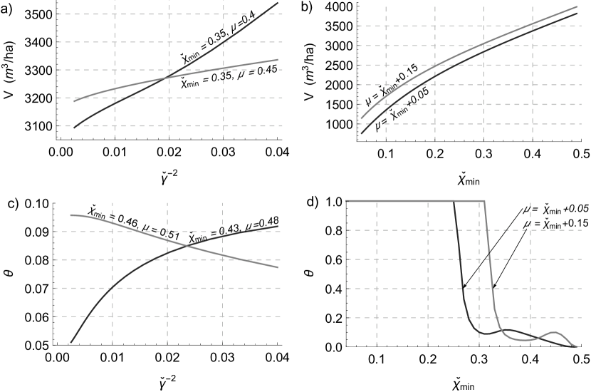
Figure 4: In the case of stochastic control, Eqs. (38) and (39), examples of a) the volume of irrigation water as a function of the process noise $\check{\gamma}^{-2}$ where $\sigma^{2}=0.75\>\check{\gamma}^{-2}$ b) the volume of irrigation water in terms of the irrigation noise setpoints represented by $\check{\chi}_{\min}$ and $\mu$. c) the effective water stress, $\Theta$, as a function of the process noise $\check{\gamma}^{-2}$ where $\sigma^{2}=0.75\>\check{\gamma}^{-2}$, and d) the effective stress as a function of the irrigation noise setpoints represented by $\check{\chi}_{\min}$ and $\mu$. Unless stated otherwise $\check{\chi}_{\min}=0.35$, $w_{o}=$ 450 mm, $k=$0.12, $E_{0}=-$4 mm/d, $\beta=0.25$, $\alpha=$10 mm, $\gamma=w_{o}/\alpha$, $\lambda=$0.15 d^-1, $\check{\gamma}=100$, $\mu=0.4$, $\sigma=0.015$, $\chi_{\max}^{+}=1$, $\varpi=0.5$, $T_{s}=$120 d, $\phi$=2, and $f=0.9$. In all instances, the crossing frequency is zero at $\check{\chi}_{\min}$, i.e., $\upsilon(\check{\chi}_{\min})=0$, and $\langle\check{\lambda}\rangle$ may be calculated from Eq. (18).

The volume of required irrigation water varies with both the control noise, as shown by the variances $\check{\gamma}^{-2}$ and $\sigma^{2}$ (Fig. 1d), and the range of the control setpoints. The range of the control setpoints approximately is indicated by $\check{\chi}_{\min}$, which represents the lower bound of the antecedent state (the ‘on’ setpoint) and $\mu$, which represents the average renewal state (the ‘off’ setpoint). As the noise increases, the average volume of irrigation water increases more for a smaller versus a larger on/off setpoint range, as roughly indicated by the difference between $\mu$ and $\check{\chi}_{\min}$ (Fig. 4a). As shown on Fig. 4a, beyond the noise (variance) of $\check{\gamma}^{-2}\approx 0.02$, the larger range of irrigation on/off setpoints proves more effective in reducing the volume of irrigation water. Such a behavior occurs because the smaller range of on/off setpoints results in a greater frequency of irrigation as the noise increases. Thus if the farmer or operator cannot precisely control irrigation, it may be more efficient (water wise) to base irrigation on a larger setpoint range with typically large water applications per irrigation event.

Not surprisingly, as the location of the on/off setpoint range increases, more irrigation water is required because the soil moisture is being maintained at values where evapotranspiration is greater (4b). The application of irrigation water must be balanced against the benefit it provides in reducing plant water stress, $\theta$, which is considered in terms of the control process noise. Depending on the on/off setpoint range, the control noise (i.e., the variances $\check{\gamma}^{-2}$ and $\sigma$) may either increase or decrease the effective plant stress (Fig. 4c). Both trends are observed because the effective stress has a minimum value with respect to the location of the on/off setpoints (Fig 4d). Naturally, the larger setpoint range and thus greater water application per irrigation event reduces the effective stress (black line, Fig 4d). Notice that the effective stress sharply decreases with the irrigation setpoint range (Fig 4d). Accordingly, an optimal irrigation control accounts for the inherent noise in the process (Figs. 4a,c) and provides a setpoint range that both minimizes the volume of irrigation water (Fig. 4c) and risk of crop failure as measured by the effective stress (Fig. 4d).

IV Conclusions

We have considered the problem of stochastic jumps with control based on setpoints. A novel formulation of the master equation, based on the mean frequency of jumps of the control process as well as the distributions of the initial and target set-points, permits constructing a master equation where the control appear more transparently than the common formulations with transition probabilities. The steady state solution is expressible in terms of a potential function and a setpoint function, which contains the properties of the control.

We have shown an application to the problem of irrigation, but similar applications can be carried out in other more complex settings also with multiple controls and redundancies. Such extensions will be presented elsewhere. We also plan to analyze the connections with stochastic thermodynamics of small systems where fluctuations appear as jumps and for which optimal stochastic controls may be especially interesting Muratore-Ginanneschi et al. (2013); Brandner et al. (2015).

Appendix A Master Equation Solution

For the master equation (13) with exponentially distributed input, $p_{z}(z)=\gamma e^{-\gamma z}$, we now derive the steady state solution $p_{\chi}(\chi)$. To this purpose, we perform a change of variables based on the Stratonovich jump prescription, i.e.:

$$y=\eta(\chi)=\int\frac{1}{b(\chi)}d\chi~{},~{}~{}\mbox{ so that }~{}~{}\chi=\eta^{-1}(y),$$ (43)

so that the corresponding transformed PDF is given by $p_{\chi}(\chi,t)=p_{y}(y,t)\left|\frac{dy}{d\chi}\right|$ and the master equation (2) takes the form

$${\partial_{t}}p_{y}(y,t)=\partial_{y}(J_{m}(y,t)+J_{\varphi}(y,t))+\langle\check{\lambda}\rangle(p_{y^{+}}(y,t)-p_{y^{-}}(y,t)).$$ (44)

We then expand Eq. (44) by substituting the probability current terms, i.e.,

$$\frac{\partial}{\partial t}p_{y}(y,t)=-\frac{\partial}{\partial y}\left[\frac{m\left(\eta^{-1}(y)\right)}{b(\eta^{-1}(y))}p_{y}(y,t)\right]-\lambda\left(\eta^{-1}(y),t\right)p_{y}(y,t)$$

$$+\int_{0}^{y}\lambda(\eta^{-1}(u),t)p_{z}\left(y-u\right)p_{y}(u,t)du$$

$$+\frac{d\chi}{dy}\delta\left(\eta^{-1}(y)-\chi_{\max}^{+}\right)\int_{\chi_{\min}}^{\chi_{\max}}\lambda(u,t)\int_{\eta(\chi_{\max}^{+})-\eta(u)-(\chi_{\max}^{+}-u)}^{\infty}p_{z}(1+q-u)p_{\chi}(u,t)dqdu$$

$$+\langle\check{\lambda}\rangle(\check{p}_{y^{+}}(y,t)-\check{p}_{y^{-}}(y,t)).$$ (45)

Assuming steady state conditions and exponential PDF of $z$, we multiply the equation by the integrating function $e^{\gamma y}$, and differentiate with respect to $y$, i.e.,

$$-e^{\gamma y}\frac{d^{2}}{dy^{2}}\left[\frac{m\left(\eta^{-1}(y)\right)}{b(\eta^{-1}(y))}p_{y}(y)\right]-e^{\gamma y}\gamma\frac{d}{dy}\left[\frac{m\left(\eta^{-1}(y)\right)}{b(\eta^{-1}(y))}p_{y}(y)\right]-e^{\gamma y}\frac{d}{dy}[\lambda\left(\eta^{-1}(y)\right)p_{y}(y)]$$

$$=e^{\gamma y}\langle\check{\lambda}\rangle\left(\gamma\check{p}_{y^{-}}(y)+\frac{d}{dy}\check{p}_{y^{-}}(y)-\gamma\check{p}_{y^{+}}(y)-\frac{d}{dy}\check{p}_{y^{+}}(y)\right).$$ (46)

Note that in steady state, the effect of an upper bound, i.e., the fourth term on the r.h.s. of Eq. (45), is accounted for in the normalization constant of the solution PDF Rodríguez-Iturbe and Porporato (2004). Dividing both sides of (46) by $e^{\gamma y}$ and integrating,

$$-\frac{d}{dy}\left[\frac{m\left(\eta^{-1}(y)\right)}{b(\eta^{-1}(y))}p_{y}(y)\right]-\frac{m\left(\eta^{-1}(y)\right)}{b(\eta^{-1}(y))}p_{y}(y,t)\left(\gamma+\lambda\left(\eta^{-1}(y)\right)\frac{b(\eta^{-1}(y))}{m\left(\eta^{-1}(y)\right)}\right)$$

$$=\langle\check{\lambda}\rangle\left(\gamma\int\check{p}_{y^{-}}(y)dy+\check{p}_{y^{-}}(y)-\gamma\int\check{p}_{y^{+}}(y)dy-\check{p}_{y^{+}}(y)\right).$$ (47)

Multiplying both sides by the integrating function

$$\exp{\int\left(\gamma+\lambda\left(\eta^{-1}(y)\right)\frac{b(\eta^{-1}(y))}{m\left(\eta^{-1}(y)\right)}\right)dy},$$

and integrating, after rearranging terms one obtains the desired solution in terms of the transformed variable,

$$p_{y}(y)=-\frac{b(\eta^{-1}(y))}{m\left(\eta^{-1}(y)\right)}e^{-\int\left(\gamma+\lambda\left(\eta^{-1}(y)\right)\frac{b(\eta^{-1}(y))}{m\left(\eta^{-1}(y)\right)}\right)dy}$$

$$\left(N+\langle\check{\lambda}\rangle\int\left(\gamma\int\check{p}_{y^{-}}(y)dy+\check{p}_{y^{-}}(y)-\gamma\int\check{p}_{y^{+}}(y)dy-\check{p}_{y^{+}}(y)\right)e^{\int\left(\gamma+\lambda\left(\eta^{-1}(y)\right)\frac{b(\eta^{-1}(y))}{m\left(\eta^{-1}(y)\right)}\right)dy}dy\right).$$ (48)

Changing variables again, the solution of Eq.(48) can be given in terms of $\chi$, as in (14).

Appendix B Jump Transition Determined for Exponential Antecedent PDF

For Eq. (10) based on $\check{p}_{\Delta\chi|u}(\Delta\chi,t)=\check{p}_{\Delta\chi}(\chi-u,t)$, we retrieve the PDF $\check{p}_{\Delta\chi}(\chi-u,t)$ when the antecedent PDF, $\check{p}_{\chi^{-}}(\chi,t)$, is based on a truncated exponential PDF, i.e.,

$$N\check{p}_{\chi^{+}}(\chi,t)=\int_{0}^{\chi}\check{p}_{\Delta\chi}(\chi-u,t)\frac{\check{\gamma}(t)e^{-\check{\gamma}(t)(u-\check{\chi}_{\min})}}{1-e^{-\check{\gamma}(t)(\check{\chi}_{\max}^{-}-\check{\chi}_{\min})}}\Theta(u-\check{\chi}_{\min})\Theta(\check{\chi}_{\max}^{-}-u)du,$$ (49)

where $\check{p}_{\chi^{-}}(u,t)$ now is defined by a truncated exponential distribution, and $N$ is the normalization constant such that

$$N=\frac{1}{\int_{\check{\chi}_{\min}+\Delta\chi_{\min}}^{\check{\chi}_{\max}^{-}+\Delta\chi_{\max}}\check{p}_{\chi^{+}}(\chi,t)d\chi},$$ (50)

for which $\Delta\chi_{\min}$ and $\Delta\chi_{\max}$ are the respective minimum and maximum jump transitions. We may pose Eq. (49) as

$$N\check{p}_{\chi^{+}}(\chi,t)=\int_{\check{\chi}_{\min}}^{\chi}\check{p}_{\Delta\chi}(\chi-u,t)\frac{\check{\gamma}(t)e^{-\check{\gamma}t)(u-\check{\chi}_{\min})}}{1-e^{-\check{\gamma}(t)(\check{\chi}_{\max}^{-}-\check{\chi}_{\min})}}du,$$ (51)

where the Heaviside step functions of Eq. (49) now are implicit in the both the integral limits and in the support of $p_{\chi^{+}}(\chi,t)$ over the range $\check{\chi}_{\min}+\Delta\chi_{\min}\leq\chi\leq\check{\chi}_{\max}^{-}+\Delta\chi_{\max}$ as indicated by the normalization constant. Following a substitution for $\chi=\Delta\chi+\check{\chi}_{\min}$ and then a change of variables based on $u=\Delta\chi+\check{\chi}_{\min}-\upsilon$ (Bendat and Piersol, 2011), Eq. (51) becomes

$$N\check{p}_{\chi^{+}}(\Delta\chi+\check{\chi}_{\min},t)=\int_{0}^{\Delta\chi}\check{p}_{\Delta\chi}(\upsilon,t)\frac{\check{\gamma}(t)e^{-\check{\gamma}(t)(\Delta\chi-\upsilon)}}{1-e^{-\check{\gamma}(t)(\check{\chi}_{\max}^{-}-\check{\chi}_{\min})}}d\upsilon.$$ (52)

After multiplying both sides of Eq. (52) by $e^{\check{\gamma}(t)\Delta\chi}$ and then differentiating with respect to $\Delta\chi$, we recover

$$\check{p}_{\Delta\chi}(\Delta\chi,t)=\frac{N\left(1-e^{-\check{\gamma}(t)(\check{\chi}_{\max}^{-}-\check{\chi}_{\min})}\right)\partial_{\Delta\chi}\left[\check{p}_{\chi^{+}}(\Delta\chi+\check{\chi}_{\min},t)e^{\check{\gamma}(t)\Delta\chi}\right]}{\check{\gamma}(t)e^{\check{\gamma}(t)\Delta\chi}},$$ (53)

where $\Delta\chi_{\min}\leq\Delta\chi\leq\Delta\chi_{\max}$ for which the limiting values of $\Delta\chi_{\min}$ and $\Delta\chi_{\max}$ respectively are found by solving $\check{p}_{\Delta\chi}(\Delta\chi_{\min})=0$ and $\check{p}_{\Delta\chi}(\Delta\chi_{\max})=0$.

We also consider the case where the PDF $\check{p}_{\Delta\chi}(\Delta\chi,t)$ and thus jump transition, $\Delta\chi$, are restricted to positive values, i.e., $\Delta\chi_{\min}=0$. Accordingly, for only positive transitions, we must restrict the maximum antecedent value, $\check{\chi}_{\max}^{-}$. The new restricted value of $\check{\chi}_{\max}^{-}$ must be consistent with the normalization condition, i.e., $\int_{0}^{\Delta\chi_{\max}}\check{p}_{\Delta\chi}(\Delta\chi)d\Delta\chi=1$. We pose the normalization condition as

$$\frac{\left(1-e^{-\check{\gamma}(t)(\check{\chi}_{\max}^{-}-\check{\chi}_{\min})}\right)}{\int_{\check{\chi}_{\min}}^{\check{\chi}_{\max}^{-}+\Delta\chi_{\max}}\check{p}_{\chi^{+}}(\chi,t)d\chi}=\frac{1}{\int_{0}^{\Delta\chi_{\max}}\frac{\partial_{\Delta\chi}\left[\check{p}_{\chi^{+}}(\Delta\chi+\check{\chi}_{\min},t)e^{\gamma(t)\Delta\chi}\right]}{\check{\gamma}(t)e^{\check{\gamma}(t)\Delta\chi}}d\Delta\chi}$$ (54)

and then find the maximum permissible value of $\check{\chi}_{\max}^{-}$ for which both sides of the equation are equal.