Random coefficient autoregressive processes describe Brownian yet non-Gaussian diffusion in heterogeneous systems

Abstract

Many studies on biological and soft matter systems report the joint presence of a linear mean-squared displacement and a non-Gaussian probability density exhibiting, for instance, exponential or stretched-Gaussian tails. This phenomenon is ascribed to the heterogeneity of the medium and is captured by random parameter models such as "superstatistics" or "diffusing diffusivity". Independently, scientists working in the area of time series analysis and statistics have studied a class of discrete-time processes with similar properties, namely, random coefficient autoregressive models. In this work we try to reconcile these two approaches and thus provide a bridge between physical stochastic processes and autoregressive models. We start from the basic Langevin equation of motion with time-varying damping or diffusion coefficients and establish the link to random coefficient autoregressive processes. By exploring that link we gain access to efficient statistical methods which can help to identify data exhibiting Brownian yet non-Gaussian diffusion.

1 Introduction

Brownian motion, one of the most fundamental processes in non-equilibrium statistical physics, describes the motion of a passive colloidal particle in a thermal fluid environment. It was observed even in ancient times, for instance, by Roman philosopher Lucretius [1]. The modern scientific interest was started by botanist Robert Brown [2]; it was later studied theoretically by Einstein, Sutherland, Smoluchowski, and Langevin between 1905 and 1908 [3, 4, 5, 6]. Two fundamental properties are typically associated with Brownian motion, namely, the linear growth

$$\delta_{X}^{2}(t)\mathrel{\mathop{:}}=\mathbb{E}[X(t)^{2}]=2Dt$$ (1)

in time of the mean-squared displacement (MSD) with the diffusion coefficient $D$, and the Gaussian probability density function (PDF)

$$p_{X}(x;t)=\frac{1}{\sqrt{4\pi Dt}}\exp\mathopen{}\mathclose{{}\left(-\frac{x^{2}}{4Dt}}\right).$$ (2)

Alternatively to the MSD (1) Brownian motion is characterised by a $1/f^{2}$ frequency dependence of the associated ensemble and single trajectory power spectra [7, 8].

Deviations from the linear time dependence (1) of the MSD are observed routinely in a large variety of systems, in particular, in the power-law form

$$\delta_{X}^{2}(t)\sim D_{\alpha}t^{\alpha}$$ (3)

with the anomalous diffusion coefficient $D_{\alpha}$ [9, 10, 11]. In biological cells or other complex liquids both subdiffusion with $0<\alpha<1$ [12, 13, 14, 15, 16, 17] and superdiffusion with $1<\alpha<2$ [18, 19, 20] are measured, see the recent reviews [21, 22]. Anomalous diffusion are effected when the increments of the stochastic process are no longer independent, when the variance of the step length or the mean-step time diverges, as well as due to the tortuosity of the embedding space. The associated PDF of these processes may have both Gaussian and non-Gaussian shapes [9, 10, 11].

Of late, a new class of diffusive dynamics has come into focus, following numerous reports in soft matter, biological and other complex systems: in these systems the MSD is normal of the form (1) with invariable coefficient $D$, however, the PDF is non-Gaussian and often found to be of the distinct exponential shape ("Laplace distribution")

$$p_{X}(x;t)=\frac{1}{\sqrt{2Dt}}\exp\mathopen{}\mathclose{{}\left(-\sqrt{\frac{2}{Dt}}|x|}\right),$$ (4)

see [23, 24, 25, 26, 27] as well as the extensive list of references in [28]. These "Brownian yet non-Gaussian" processes along with a more general class of non-Gaussian PDFs, discussed in more detail below, are in the focus of this study.

Our goal here is, however, different from the previous modelling approaches. Namely, here we try to establish a direct connection of the physical models for Brownian yet non-Gaussian diffusion and a class of processes ubiquitously used in time series analysis, the so-called autoregressive models with random coefficients [29, 30, 31].

Thus, we introduce the time series methods to the modeling of non-Gaussian diffusion, which enables us to provide information about the distribution of the process, showing the influence of some effective properties of the heterogeneous medium. In particular it allows to distinguish between locally homogeneous (”superstastics” type) and rapidly varying (”diffusing diffusivity” type) environments (see, e.g. figure 2). It also makes it possible to show how the heterogeneity of the original Langevin model induces the non-linear memory structure of the studied process, which is visible in the simulated data.

The work is structured as follows: in section 2 we provide more information on the process of Brownian yet non-Gaussian diffusion along with a primer to autoregressive models. Section 3 then introduces an intuitive physical derivation of the autoregressive model. The situation when the correlation times of the random diffusion coefficients is comparatively short is then considered in detail in section 4. In section 5 we show how the statistical methods of time series can be used to qualify and quantify the non-Gaussianity. There, we also use the analytical formulas for moments to detect the non-linear memory structure specific to the considered model. We summarise our results and discuss their utility in section 6. The paper closes with an appendix, in which the derivation of the moments is presented.

2 Physical stochastic modelling and autoregressive models

2.1 Brownian yet non-Gaussian diffusion

In the original works on Brownian yet non-Gaussian diffusion the linear MSD (1) was observed along with the Laplace shape (4) of the PDF. Other findings suggest the presence of more general stretched Gaussian tails

$$p_{X}(x;t)\propto\exp\mathopen{}\mathclose{{}\left(-\mathopen{}\mathclose{{}\left(\frac{|x|}{ct^{\alpha/2}}}\right)^{\delta}}\right),$$ (5)

with the stretching parameter $\delta\neq 2$. PDFs of this type describe diffusion that can be normal ($\alpha=1$) or anomalous of the form (3) with $\alpha\neq 1$. It was found that $\delta=1$ and $\alpha$ between 0.75 and 0.25 for tracer diffusion in living bacteria and eukaryotic cells [32]. Similarly, in simulations of crowded membranes it was shown that $\delta$ is between 1.3 and 1.6, and $\alpha$ below 1 [33].

This behaviour can be explained by the fact that the considered medium is spatially or temporally heterogeneous [23, 24, 28, 35, 36, 37]. In such a system the thermal fluctuations are still Gaussian but the observed displacements are mixtures of these Gaussian contributions with random weights, effecting the non-Gaussian outcome. In practice, this is commonly realised by two classes of diffusion models, namely by so-called "superstatistics" and "diffusing diffusivity" models.

Superstatistics is a term proposed by Cohen and Beck [38, 39, 40] and stands for superposition of statistics. It refers to a model with random parameters, that are fixed for each trajectory. This is a form of hierarchical or multilevel modelling [41], which is also close to the Bayesian inference method. The distributions which arise this way are called compound or mixture [42]. In the context of diffusion this mixture approach can be explained in the following way: each observed trajectory either moves in its own neighbourhood, that has distinct properties affecting the motion. These features are supposed to not vary significantly at temporal and spatial scales specific to the observed trajectories. If the motion is not confined, this assumption must be viewed as a short-time approximation. Another possible origin is the situation when the diffusion characteristics of the observed particles vary from one to another, for instance, the radius of different tracer beads. In this case the compound distributions are observed at long times, as well, but this possibility can be excluded for experiments in which the type of the diffusing object is precisely controlled.

The simplest type of a mixture model is Brownian diffusion with a randomised, but global diffusion coefficient $D$. In it, the infinitesimal increments of the position process are given by

$$\mathrm{d}X(t)=\sqrt{D}\mathrm{d}B(t),\quad$$ (6)

where $B$ represents standard Brownian motion. If we assume that $D$ has an exponential distribution, the emerging process is characterised by the Laplace PDF (4). Similarly, a stretched exponential PDF of $D$ leads to relation (5). The randomness of $D$ was confirmed in many experiments [26, 32, 37] and also in numerical studies [33]. Since there is no fundamental reason to pinpoint the diffusion coefficient as the only heterogeneous property of the system, other parameters can also be made superstatistical. For example, a random viscosity or memory kernel in the Langevin equation also lead to non-Gaussian PDFs and generally non-linear MSD [43]. It must be stressed that by introducing a parameter which is random and fixed trajectory-wise, we break not only homogeneity, but also locality and independence. By sharing the same random parameter, the memory structure of the process becomes non-linear and non-Gaussian [43]. This dependence is strong enough to render the resulting motion non-ergodic.

This non-ergodic property is not always desired and can be avoided when the system parameters are allowed to be both random and time-dependent, as in the diffusing diffusivity model. Fixed, deterministic values are replaced by a stochastic variation of the parameter, and for this reason the resulting models are called doubly stochastic [44]. If the introduced parameter evolution is ergodic, the resulting model will be ergodic, but still non-Gaussian. For example, one can consider a time-varying diffusion coefficient leading to the diffusing diffusivity approach proposed by Chubinsky and Slater [45]. In this model small Brownian displacements $\mathrm{d}B(t)$ are assumed to be randomly rescaled by random $D(t)$, such that the resulting motion is described by the stochastic equation

$$\mathrm{d}X(t)=\sqrt{D(t)}\mathrm{d}B(t)\quad\text{or equivalently}\quad X(t)=\int_{0}^{t}\sqrt{D(s)}\mathrm{d}B(s).$$ (7)

Further details of the process depend on the specific choice of $D(t)$—the analysis is often complicated. However, an important case was solved by Cox, Ingerson and Ross [49] who proposed a stochastic differential equation with suitable mean-reverting property that leads to $D(t)$ with exponential type of memory. Their work was motivated by financial applications and was expressed in the language of option prices and volatility modelling. More recently, this approach was applied to physically relevant quantities in [28, 35, 50, 51, 52], in particular, for non-stationary initial conditions [34].

2.2 Autoregressive models

In contrast to models originating from physics, autoregressive models have their roots in filtering, optimal control theory, and economics [29]. In this context the measured sequence of observations $V_{k}$ is assumed to be an output of a system, which is linked linearly to the white Gaussian noise input sequence $Z_{k}$. The classical autoregressive moving average (ARMA) processes [30, 31] are defined by the recursive relation

$$V_{k}-\phi^{1}V_{k-1}+\phi^{2}V_{k-2}+\ldots\phi^{p}V_{k-p}=Z_{k}+\theta^{1}Z_{k-1}+\theta^{2}Z_{k-2}+\ldots+\theta^{q}Z_{k-q}.$$ (8)

This process is denoted by ARMA$(p,q)$ and thus explicitly contains the range parameters $p$ and $q$. The term autoregressive AR($p$) reflects the linear dependence of the observed $V_{k}$ on $p$ past values $V_{k-1},\ldots,V_{k-p}$, and the moving average MA($q$) represents a linear combination of the last value of the noise $Z_{k}$ and $q$ previous values $Z_{k-1},\ldots,Z_{k-q}$. The admissible coefficients $\phi^{i}$ and $\theta^{j}$ are chosen such that the sequence $V_{k}$ is stationary, resembling the physical velocity process (hence the choice of notation "$V$") or highly confined motion.

In most of the literature the model (8) was not meant to explain the behaviour of the system. Rather, the philosophy was concentrated on controlling the data. This can be achieved by finding a reasonably small set of $\phi^{i}$ and $\theta^{j}$ that sufficiently well describe the observed memory structure in the data. The procedure typically employs methods based on mean-square optimisation and information theory [30, 31]. Given the estimates of the $\phi^{i}$ and $\theta^{j}$ the future behaviour can be predicted (in the sense of the least square error or similar), which is a crucial element, for instance, in financial forecasting. Additionally, by inverting relation (8), the $Z_{k}$ can be estimated from the $V_{k}$, therefore various white noise tests can be used to verify the goodness of fit of the model [31].

It is in fact remarkable how many concepts of non-equilibrium and biological physics have their independent counterparts in time series analysis. For example, the study of anomalous diffusion and long-range dependence can be performed by using autoregressive fractionally integrated (ARFIMA) models where the white noise sequence $Z_{k}$ is replaced by the fractional noise $Z_{k}^{d}$ [53, 54] with a power-law covariance structure determined by the parameter $d$, $\mathbb{E}[Z_{k}^{d}Z_{k+j}^{d}]\propto j^{2d-1}$ (one can think of $d$ as Hurst exponent minus 1/2). It can be explicitly defined as the result of the power-law filter applied to $Z_{k}$,

$$Z_{k}^{d}=\sum_{j=1}^{\infty}\frac{\Gamma(j+d)}{\Gamma(d)\Gamma(j+1)}Z_{k-j}.$$ (9)

For ARMA processes, the left hand side of (8)—the AR part— is responsible for modelling an exponential decay of the covariance, whereas the MA part introduces short, finite time corrections. Additional filtering of the white noise presented in (9) extends the ARMA model to the ARFIMA with power-law memory, which was very successfully applied to various anomalous diffusion phenomena encoded in biological data [55]. An analogue of Lévy flights and diffusion with a power-law PDF is the ARMA model with stable noise, where the Gaussian $Z_{k}$ are replaced by non-Gaussian stable random variables [56]. Similarly, fractional Lévy stable motion corresponds to ARFIMA with stable noise [57, 54].

Another line of development in time series analysis, originating from Box-Jenkins models, are non-linear generalisations, mainly the so-called autoregressive conditional heteroscedasticity (ARCH) [58] and generalised ARCH (GARCH) models [59]. These allow for the parameterisation and prediction of a non-constant variance and proved to be very useful for financial time series; their invention prompted the bestowal of the Nobel Memorial Prize in Economic Sciences in 2003 to Granger and Engle. When integrated ARCH-type processes exhibit non-Gaussian distributions for short times along with a linear time dependence of the MSD. Precisely this observation leads us to pursue the question whether there is a fundamental connection between the two worlds of time series analysis using autoregressive methods and physical models of Brownian yet non-Gaussian type.

The aforementioned notion of heteroscedasticity is related to the time-dependence of the conditional variance [60, 61]. The basic ARCH$(q$) model is defined as

$$V_{k}=\Sigma_{k}Z_{k},\quad\Sigma_{k}^{2}=\alpha_{0}+\alpha_{1}V_{k-1}^{2}+\alpha_{2}V_{k-2}^{2}+\ldots+\alpha_{q}V_{k-q}^{2}.$$ (10)

If an ARMA model is assumed for the noise variance, the model becomes a GARCH$(p,q)$ model,

$$V_{k}=\Sigma_{k}Z_{k},\quad\Sigma_{k}^{2}=\alpha_{0}+\sum_{i=1}^{q}\alpha_{i}V_{k-i}^{2}+\sum_{j=1}^{p}\beta_{j}\Sigma_{k-j}^{2}.$$ (11)

A GARCH model has an ARMA-type representation, so that many of its properties are similar to those of ARMA models, for instance, we can estimate the GARCH parameters by the same technique as for ARMA processes [29]. In most applications it is enough to consider the order of the model as $(1,1)$. ARFIMA combined with GARCH describes both power-law decay of the correlation function with finite-lag effects (ARFIMA part) and varying diffusion parameter (GARCH part) [62]. For example, it can describe inhomogeneous diffusion in the cell membrane [63] or solar X-ray variability [64]. While the resemblance to diffusing diffusivity models (7) is indisputable: $V_{k}$ models velocity and $\Sigma_{k}$ models the evolving diffusion coefficient, there is to date no physical derivation of relations (10) and (11).

Another approach related to heteroscedasticity, non-Gaussianity and linear MSD is the main point of interest in this work: we assume that the linear coefficients $\phi^{i}$ and $\theta^{j}$ in the definition of ARMA (8) are replaced by random variables $\Phi_{k}^{i}$ and $\Theta_{k}^{j}$ that are independent of the noise $Z_{k}$:

$$V_{k}-\Phi_{k}^{1}V_{k-1}+\Phi_{k}^{2}V_{k-2}+\ldots\Phi_{k}^{p}V_{k-p}=\Theta_{k}^{0}Z_{k}+\Theta_{k}^{1}Z_{k-1}+\Theta_{k}^{2}Z_{k-2}+\ldots+\Theta_{k}^{q}Z_{k-q}.$$ (12)

This is the class of doubly stochastic models, random coefficient ARMA (rcARMA) [65, 66].

3 Physical derivation of the autoregressive model

Let us start with the classical Langevin equation for the velocity of a diffusing particle,

$$m\frac{\mathrm{d}V(t)}{\mathrm{d}t}=-\beta V(t)+F(t),$$ (13)

which is Newton’s second law with the Stokes dissipative force $-\beta V$ and the stochastic force $F$. In the classical setting $F$ is given by white Gaussian noise with amplitude $k_{B}T\beta$ determined by the fluctuation-dissipation relation [67, 68]. Heterogeneity of the medium can be modelled by making the parameters of equation (13) time-dependent and random—then they describe the local state of the environment of the diffusing particle. All possible correlation effects caused by the particle repeatedly visiting the same areas of the phase space are assumed to be reflected by the memory structure of random functions modelling these local parameters. Starting from the next section we will neglect this dependence entirely, which corresponds to an annealed picture that is also inherent in the current physical diffusing diffusivity models.This assumption can be also justified when the environment changes continuously. The resulting equation can then be written in the form

$$\mathrm{d}V(t)=-\Lambda(t)V(t)\mathrm{d}t+\sqrt{D(t)}\mathrm{d}B(t).$$ (14)

We do not provide any more fundamental derivation behind this formula, for us $\Lambda(t)$ and $D(t)$ are effective parameters whose physical meaning is determined by equation (14) alone: $D(t)$ describes the local effective amplitude of velocity gains and $\Lambda(t)$ the local effective linear damping or relaxation of the velocity. In financial language these parameters would be called stochastic return rate and stochastic volatility. Take note this class of models differs from the superstatistical approach of Beck and Cohen [38], who assume the Langevin dynamics and stochasticity of environement can be considered separately. In (30) we consider a particular case leading to superstatistics.

Formula (14) resembles the rcARMA. Indeed, in the standard Euler scheme of numerical simulations, one fixes a time delay $\Delta t$ between observations, denotes $V_{k}=V(k\Delta t)$ and approximates $\mathrm{d}V(t)\approx V_{k}-V_{k-1}$, which results in

$$V_{k}-(1-\Lambda_{k}\Delta t)V_{k-1}=\sqrt{D_{k}}\Delta B_{k}.$$ (15)

This is an rcAR(1) process with AR coefficient $1-\Lambda_{k}\Delta t$. It is easy to see that the same reasoning applies to any linear stochastic differential equation and thus the classical schemes of discrete-time simulations return rcARMA processes approximating the continuous-time solutions.

In fact, the connections between rcARMA and models of diffusing diffusivity reach deeper than that. Classical results from the theory of time series analysis establish that there is an exact correspondence between ARMA and solutions of linear stochastic equations with constant coefficients—no approximation is needed [69]. The classical Langevin equation for a position of a particle confined in an harmonic potential,

$$m\frac{\mathrm{d}^{2}X(t)}{\mathrm{d}t^{2}}=-\kappa X(t)-\beta\frac{\mathrm{d}X(t)}{\mathrm{d}t}+F(t)$$ (16)

fits into this category. The resulting discrete motion is the ARMA(2,1) process

$$X_{k}-\phi^{1}X_{k-1}-\phi^{2}X_{k-2}=Z_{k}+\theta Z_{k-1}$$ (17)

with AR(2) coefficients

$$\phi^{1} =\rme^{-\Delta t\frac{\beta}{2m}}\mathopen{}\mathclose{{}\left(\rme^{\Delta t\sqrt{\mathopen{}\mathclose{{}\left(\frac{\beta}{2m}}\right)^{2}-\frac{\kappa}{m}}}+\rme^{-\Delta t\sqrt{\mathopen{}\mathclose{{}\left(\frac{\beta}{2m}}\right)^{2}-\frac{\kappa}{m}}}}\right),$$

$$\phi^{2} =-\rme^{-\Delta t\frac{\beta}{m}}.$$ (18)

The MA(1) coefficient $\theta$ can be easily calculated numerically or expressed by a somewhat complicated but elementary formula [70]. This class of relations has direct application to the statistical analysis of the data and can be used, for instance, to calculate the exact discrete-time power spectral density (the spectrum given by the Fourier series of $X_{k}$) without the need of the commonly used approximation $\sum_{k}f(X_{k})\Delta t\approx\int f(X(t))\mathrm{d}t$ [71].

The core of the physical interpretation we propose in this work is that the derivation used to obtain (16) and (17) can be generalised for the case of linear equations with time-dependent coefficients. Namely, we multiply (14) by the integrating factor $\exp(\int\Lambda(t)\mathrm{d}t)$ and integrate from $(k-1)\Delta t$ to $k\Delta t$, obtaining

$$\rme^{\int_{0}^{k\Delta t}\Lambda(s)\mathrm{d}s}V_{k}-\rme^{\int_{0}^{(k-1)\Delta t}\Lambda(s)\mathrm{d}s}V_{k-1}=\int_{(k-1)\Delta t}^{k\Delta t}\rme^{\int_{0}^{s}\Lambda(s^{\prime})\mathrm{d}s^{\prime}}\sqrt{D(s)}\mathrm{d}B(s).$$ (19)

After some rearrangement it takes the sleek form

$$V_{k}-\Phi_{k}V_{k-1}=Z_{k}$$ (20)

with

$$\Phi_{k}\mathrel{\mathop{:}}=\rme^{-\int_{(k-1)\Delta t}^{k\Delta t}\Lambda(s)\mathrm{d}s},\quad Z_{k}\mathrel{\mathop{:}}=\int_{(k-1)\Delta t}^{k\Delta t}\rme^{-\int_{s}^{k\Delta t}\Lambda(s^{\prime})\mathrm{d}s^{\prime}}\sqrt{D(s)}\mathrm{d}B(s).$$ (21)

The random coefficient AR form of the left hand side is clearly present, but it is not immediately clear what is the structure of $Z_{k}$ on the right. Different $Z_{k}$ use increments $\mathrm{d}B(s)$ from disjoint intervals $[(k-1)\Delta t,k\Delta t]$. The Gaussian increments $\mathrm{d}B(s)$ are stationary and do not depend on $k$ but they are rescaled by $D(t)$ and the exponent of $\Lambda(t)$, which makes their conditional variances a sequence of random variables,

$$\mathbb{E}[Z_{k}^{2}|\Lambda,D] =\int_{(k-1)\Delta t}^{k\Delta t}\mathopen{}\mathclose{{}\left(\rme^{-\int_{s}^{k\Delta t}\Lambda(s^{\prime})\mathrm{d}s^{\prime}}\sqrt{D(s)}}\right)^{2}\mathrm{d}s$$

$$=\int_{(k-1)\Delta t}^{k\Delta t}\rme^{-2\int_{s}^{k\Delta t}\Lambda(s^{\prime})\mathrm{d}s^{\prime}}D(s)\mathrm{d}s.$$ (22)

Conditioned on $\Lambda$ and $D$ the variables $Z_{k}$ are Gaussian, independent, and have the variance specified above. Thus the $Z_{k}$ can be decomposed as $Z_{k}=\Theta_{k}W_{k}$ for a Gaussian white noise $W_{k}$ and coefficients $\Theta_{k}=\sqrt{\mathbb{E}\mathopen{}\mathclose{{}\left[Z_{k}^{2}|\Lambda,D}\right]}$, which is a function of random $\Lambda(t)$ and $D(t)$. This is but exactly the rcARMA

$$V_{k}-\Phi_{k}V_{k-1}=\Theta_{k}W_{k},$$ (23)

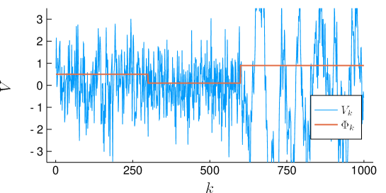
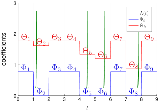
in which the regressive coefficients $0\leq\Phi_{k}\leq 1$ model the local return or relaxation rates, and the amplitude coefficients $\Theta_{k}\geq 0$ describe the heteroscedasticity of fluctuations, that is the variability of the fluctuations’ dispersion. An illustration how the changes of $\Phi_{k}$ are visible in the data can be seen in figure 1.

Figure 1: Trajectory $V_{k}$ in which $\Phi_{k}$ changes in 3 intervals from $0.5$, to $0.1$, and finally $0.9$, while $\Theta_{k}=1$ is kept constant. For small $\Phi_{k}$ the motion resembles white noise, larger values result in longer Brownian excursions away from $0$. Note that for better visibility very long excursion are cut off.

Each $\Phi_{k}$ is a decreasing functional of the values $\Lambda(t)$ from the interval $[(k-1)\Delta t,k\Delta t]$. Similarly $\Theta_{k}$ is increasing with $D(t)$ and decreasing with $\Lambda(t)$. Therefore $\Phi_{k}$ and $\Theta_{k}$ are two sequences which should mirror the memory structure of $\Lambda(t)$ and $D(t)$. They are dependent, because they both are functionals of the same range of values $\Lambda(t)$. In general the form of this dependence is highly non-linear. When the parameters can be assumed to not vary significantly in the interval $\Delta t$, $\Lambda(t)\approx\Lambda_{k}$ and $D(t)\approx D_{k}$, the approximate relation reads

$$\Phi_{k}\approx\rme^{-\Delta t\Lambda_{k}},\quad\Theta_{k}\approx\sqrt{\frac{D_{k}}{2\Lambda_{k}}}\sqrt{1-\rme^{-2\Delta t\Lambda_{k}}}\approx\sqrt{\frac{\Delta tD_{k}}{-2\ln(\Phi_{k})}}\sqrt{1-\Phi_{k}^{2}}.$$ (24)

In practical applications this formula can be further simplified. Namely, the function $(1-x^{2})/(-\ln(x))$ is approximately linear on the interval $[0,1]$, thus a reasonable approximation is $\Theta_{k}\approx\sqrt{D_{k}\Phi_{k}}$.

No matter what is the distribution of the $\Phi_{k}$ and $\Theta_{k}$, the solution of (23) itself can be expressed in a simple manner. Repeating the recursive relation between $V_{k}$ and $V_{k-1}$ we can write the explicit formula linking $V_{k}$ and $V_{k-n}$ for any $n$ in the form

$$V_{k} =\Phi_{k}\Phi_{k-1}\cdots\Phi_{k-n+1}V_{k-n}+\Theta_{k}W_{k}+\Phi_{k}\Theta_{k-1}W_{k-1}+\Phi_{k}\Phi_{k-1}\Theta_{k-2}W_{k-2}+\ldots$$

$$+\Phi_{k}\cdots\Phi_{k-n+2}\Theta_{k-n+1}W_{k-n+1}.$$ (25)

Away from the degenerate case $\Lambda(t)\equiv 0$ it is true that $\Phi_{k}<1$, therefore when $n\to\infty$ the series converges towards

$$V_{k}=\sum_{i=0}^{\infty}\Big{(}\prod_{j=0}^{i-1}\Phi_{k-j}\Big{)}\Theta_{k-i}W_{k-i}.$$ (26)

We see that each $V_{k}$ is a mixture of Gaussian variables $W_{k}$ with random weights. The result is not Gaussian, but can be characterised as conditionally Gaussian $\mathcal{N}(0,S^{2})$ with conditional variance

$$S^{2}\mathrel{\mathop{:}}=\mathbb{E}\mathopen{}\mathclose{{}\left[V_{k}^{2}|\Phi,\Theta}\right]=\sum_{i=0}^{\infty}\Big{(}\prod_{j=0}^{i-1}\Phi_{k-j}^{2}\Big{)}\Theta_{k-i}^{2}.$$ (27)

The distribution of $S^{2}$ determines the non-Gaussianity: the more spread out $S^{2}$ is, the more the PDFs of the velocity and displacement differ from the Gaussian shape. This property can be expressed in terms of the excess kurtosis, which is directly related to the relative standard deviation (RSD) of $S^{2}$. Namely,

$$\kappa_{V}\mathrel{\mathop{:}}=\frac{\mathbb{E}\mathopen{}\mathclose{{}\left[V_{k}^{4}}\right]}{\mathbb{E}\mathopen{}\mathclose{{}\left[V_{k}^{2}}\right]^{2}}-3=3\frac{\mathbb{E}\mathopen{}\mathclose{{}\left[(S^{2}-\mathbb{E}\mathopen{}\mathclose{{}\left[S^{2}}\right])^{2}}\right]}{\mathbb{E}\mathopen{}\mathclose{{}\left[S^{2}}\right]^{2}}$$ (28)

is three times the RSD squared. Different variants of the excess kurtosis or the RSD of $S^{2}$ are sometimes called "non-Gaussianity parameter" [72, 73], but here we will use more precise terminology. Because both are positive, the distribution of $V$ is always leptokurtic, that is, it has tails thicker than a Gaussian. It is worth stressing that the kurtosis is only one of many possible measures of non-Gaussianity, but it is a convenient one because of the easy estimation.

The distribution of $S^{2}$ is, in general, hard to analyse even for simple models of $\Phi$ and $\Theta$. One exception is encountered when the coefficients stay constant for long intervals of time $T_{\alpha}$ (precisely, $\mathbb{E}\mathopen{}\mathclose{{}\left[T_{\alpha}}\right]$ larger than the mean relaxation time $1/\mathbb{E}\mathopen{}\mathclose{{}\left[\Phi}\right]$). In such a situation $S^{2}$ spends short times transitioning between these periods and therefore in the majority they attain an equilibrium value obtained from taking the coefficients in (27) constant,

$$S^{2}_{\alpha}=\frac{\Theta^{2}_{\alpha}}{1-\Phi_{\alpha}^{2}},$$ (29)

where $\alpha$ is an identification of the interval. The resulting distribution of $S^{2}$ is thus

$$S^{2}\approx\frac{\widetilde{\Theta}^{2}}{1-\widetilde{\Phi}^{2}},$$ (30)

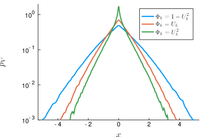
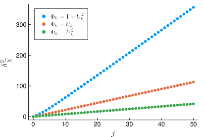
with $\widetilde{\Theta}$ and $\widetilde{\Phi}$ being random variables constructed from the values $\Theta_{\alpha},\Phi_{\alpha},\Theta_{\beta},\Phi_{\beta},\Theta_{\gamma},$ $\Phi_{\gamma},\ldots$ with probabilities weighted by the relative mean lengths of the intervals $T_{\alpha},T_{\beta},T_{\gamma},...$. In this approximation one trajectory is effectively the same as an ensemble of equal-length trajectories, each with its own $\widetilde{\Theta},\widetilde{\Phi}$, which are glued together at the ends, merging into a single trajectory. (This is essentially a form of superstatistics.) For a simple demonstration see figure 2. There one of the limiting cases are long periods of constant coefficients, as in (30), but one can also observe the second limit of rapidly varying coefficients. This is the subject of the next section.

Figure 2: PDF of the rcAR process $V$ with random periods $T_{\alpha}$ of constant coefficients $\Phi_{\alpha}$ and $\Theta_{\alpha}=1$. The dashed lines represent rcAR simulations, the solid lines correspond to theoretical predictions for the limiting cases. The distribution was chosen to be the simple geometric distribution $\mathcal{G}eo(q))$, $\mathrm{P}(\mathcal{G}eo(q))=k)=q^{k}$, and the two types of periods are chosen as $\mathrm{P}(\Phi_{\alpha}=0.1,T_{\alpha}\overset{d}{=}\mathcal{G}eo(q))=1/2$ and $\mathrm{P}(\Phi_{\alpha}=0.9,T_{\alpha}\overset{d}{=}\mathcal{G}eo(q))+\mathcal{G}eo(q))=1/2$. The periods of $\Phi_{\alpha}=0.9$ are on average twice longer, thus the effective distribution is $\mathrm{P}(\widetilde{\Phi}=0.1)=1/3$, and $\mathrm{P}(\widetilde{\Phi}=0.9)=2/3$. The prediction $q\to 1$ from (27) with independent coefficients distributed like $\widetilde{\Phi}$. The prediction $q\to 0$ comes from (30), in the latter case the PDF is just a superposition of two Gaussians.

4 Short memory random coefficient AR(1)

When the correlation time of $\Lambda(t)$ and $D(t)$ is much smaller than the observation time, $t_{c}\ll\Delta t$, the integrals defining $\Phi_{k},\Phi_{k+1}$ and $\Theta_{k},\Theta_{k+1}$ contain only the ratio $t_{c}/\Delta t$ of the total mass corresponding to dependent values of $\Lambda(t),D(t)$. Thus, $\Phi_{k}$ and $\Theta_{k}$ can be assumed to be sequences of independent and identically distributed (i.i.d.) variables. Note that for fixed $k$ the pair $\Phi_{k},\Theta_{k}$ may, and generally will be dependent. Averaging (27) yields

$$\mathbb{E}\mathopen{}\mathclose{{}\left[V_{k}^{2}}\right]=\mathbb{E}\mathopen{}\mathclose{{}\left[S^{2}}\right]=\frac{\mathbb{E}\mathopen{}\mathclose{{}\left[\Theta_{k}^{2}}\right]}{1-\mathbb{E}\mathopen{}\mathclose{{}\left[\Phi_{k}^{2}}\right]}.$$ (31)

Similarly, $\mathbb{E}\mathopen{}\mathclose{{}\left[S^{4}}\right]$ can be calculated, as detailed in the appendix. The moments $\mathbb{E}\mathopen{}\mathclose{{}\left[S^{2}}\right]$ and $\mathbb{E}\mathopen{}\mathclose{{}\left[S^{4}}\right]$ together determine the kurtosis of $V$. Accordingly, the motion is again non-Gaussian. The covariance also has a simple form: from the recursive formula (3) we can easily derive the geometric decay

$$r_{V}(j)\mathrel{\mathop{:}}=\mathbb{E}\mathopen{}\mathclose{{}\left[V_{k}V_{k+j}}\right]=\mathbb{E}\mathopen{}\mathclose{{}\left[S^{2}}\right]\varphi^{j},\quad\varphi\mathrel{\mathop{:}}=\mathbb{E}\mathopen{}\mathclose{{}\left[\Phi_{k}}\right].$$ (32)

The form of the covariance also determines the MSD: for the velocity it converges exponentially to a constant $\delta^{2}_{V}(j)=2(1-r_{V}(j))$ and for the position $X_{k}\mathrel{\mathop{:}}=\int_{0}^{k\Delta t}V(\tau)\mathrm{d}\tau$ it is linear for $j\gg 1$,

$$\delta_{X}^{2}(j)=\frac{c^{2}}{-\ln\varphi}j+\frac{c^{2}}{\ln\varphi^{2}}\mathopen{}\mathclose{{}\left(\varphi^{j}-1}\right),\quad c^{2}\mathrel{\mathop{:}}=2\Delta t^{2}\mathbb{E}\mathopen{}\mathclose{{}\left[S^{2}}\right].$$ (33)

A similar formula can be obtained if one tries to recreate displacements given $V_{k}$: then $\widetilde{X}_{k}\mathrel{\mathop{:}}=\Delta t\sum_{i=1}^{k}V_{i}$ leads to the formula

$$\delta_{\widetilde{X}}^{2}(j)=\frac{c^{2}}{2}\frac{(1+\varphi)}{1-\varphi}j-c^{2}\varphi\frac{1-\varphi^{j}}{(1-\varphi)^{2}}.$$ (34)

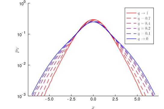
A small error in determining the slope of the true $X(t)$ is made in this procedure, but the general behaviour of the MSD is the same. Note that the shapes of all the above functions depend only on the mean value of $\Phi_{k}$, this is a diffusion with covariance and MSD (up to a scaling factor) as if the system were homogenised—however, at the same time it is non-Gaussian, see figure 3.

Figure 3: PDF and MSD estimated from the rcAR process $V$. Here $U_{k}$ are independent and uniformly distributed, $\mathcal{U}(0,1)$, and $\Theta_{k}=\sqrt{\Phi_{k}}$. Different transformations of $U_{k}$ correspond to different power laws of $\Phi_{k}$ around $0^{+}$ and $1^{-}$.

As a concrete example of a physical model which leads to this type of process let us assume that the diffusivity is constant (with no loss of generality we take $D(t)=1$). Then we consider a diffusing particle interacting with high viscosity traps distributed in a Poissonian manner, that is, the waiting time between subsequent trapping events have the exponential distribution $\mathcal{E}(\rho)$. By a high-viscosity trap we mean a short-time interval when $\Lambda(t)=\infty$, which immediately kills the momentum of the particle—this is a form of stochastic resetting [74]. Outside of these events the damping rate is constant $\Lambda(t)=\lambda$. The probability that the particle does not meet any traps between times $(k-1)\Delta t$ and $k\Delta t$ is $\exp(-\rho\Delta t)$: in this case $\Phi_{k}=\exp(-\lambda\Delta t)$ and $\Theta_{k}=\sqrt{(1-\exp(-2\lambda\Delta t))/(2\lambda)}$. The probability that the particle meets at least one trap in an interval $[(k-1)\Delta t,k\Delta t]$ is of probability $1-\exp(-\rho\Delta t)$, and the corresponding AR(1) coefficient $\Phi_{k}$ becomes 0. The discrete noise $Z_{k}$ for this $k$ has a more complex structure. All Gaussian fluctuations before the last trapping event are erased, which is visible from (21). However the remaining fluctuations still count. Denoting by $T_{k}$ the difference between the last trapping event and $k\Delta t$ we obtain the formula for $\Theta_{k}^{\prime}$ corresponding to the event $\Phi_{k}=0$,

$$\Theta_{k}^{\prime}=\sqrt{\int_{k\Delta t-T_{k}}^{k\Delta t}\rme^{-2\lambda(k\Delta t-s)}\mathrm{d}s}=\sqrt{\frac{1-\rme^{-2\lambda T_{k}}}{2\lambda}}\approx\sqrt{T_{k}}.$$ (35)

This corresponds to a small correction $\mathcal{O}(\Delta t)$, which makes the resulting PDF smooth (otherwise the trapping events would be visible as a Dirac delta at $x=0$). The approximation on the right holds for $\lambda\Delta t\ll 1$. The relation between $\Lambda(t)$ and $\Phi_{k},\Theta_{k}$ is shown in figure 4 using an exemplary trajectory.

Figure 4: Damping rate $\Lambda(t)$ and corresponding $\Phi_{k},\Theta_{k}$. Here $\Delta t=1$ and, outside of the short impulses, $\Lambda(t)=1/4$. To better highlight different values of the coefficients, the diffusion coefficient was taken to be $D(t)=4$.

Variables $T_{k}$ which determine $\Theta_{k}$ have the distribution of an exponential variable conditioned by the requirement that it has value lower than $\Delta t$ (that is, the trapping event occurred in the considered interval). It has the PDF

$$p_{T_{k}}(t)=\frac{\rho}{1-\rme^{-\rho\Delta t}}\rme^{-\rho t},\quad 0\leq t\leq\Delta t.$$ (36)

As we determined the exact distribution of $\Phi_{k}$ and $\Theta_{k}$, the formula for the covariance (32) can be made completely explicit, namely

$$r_{V}(j)=\mathbb{E}\mathopen{}\mathclose{{}\left[S^{2}}\right]\rme^{-j(\rho+\lambda)\Delta t},\quad\mathbb{E}\mathopen{}\mathclose{{}\left[S^{2}}\right]=\frac{1}{2\lambda}\frac{1+\rme^{-\rho\Delta t}-2\frac{\rho+\lambda}{\rho+2\lambda}\rme^{-(\rho+2\lambda)\Delta t}}{1-\rme^{-(\rho+2\lambda)\Delta t}}.$$ (37)

The variance $\mathbb{E}\mathopen{}\mathclose{{}\left[S^{2}}\right]$ has a complicated form, but the geometric decay rate is given by $(\rho+\lambda)\Delta t$. It is an intuitive result: meeting a trap erases the momentum of the particle, which thus loses all connection to its history at a frequency proportional to the density of traps.

Studying the distribution of $V_{k}$ in general is hard, even for i.i.d. coefficients, because the conditional variance (27) is given by an infinite sum with terms which are dependent, as the same $\Phi_{k-i}$ reappear in them. In the studied example the situation is specific and simpler, because the sum is actually finite. The coefficients $\Phi_{k-i}$ are a series of Bernoulli trials—after a series of $j-1$ non-zero ones appearing with probability $\exp(-\rho\Delta t)^{j}$ the first zero occurs with probability $1-\exp(-\rho\Delta t)$ and the summation stops. Conditioned by this event the first $j-1$ values $\Theta_{k-i}$ are deterministic, but the last term in the sum, $\Theta_{k-j}^{\prime}$ has the conditional distribution (35). This leads to the formula for characteristic function,

$$\widehat{p}_{V}(\theta) =\mathbb{E}\mathopen{}\mathclose{{}\left[\exp\mathopen{}\mathclose{{}\left(-\frac{\theta^{2}}{2}S^{2}}\right)}\right]$$ (38)

$$=\sum_{j=0}^{\infty}\mathbb{E}\mathopen{}\mathclose{{}\left[\exp\mathopen{}\mathclose{{}\left(-\frac{\theta^{2}}{2}\mathopen{}\mathclose{{}\left(\sum_{i=0}^{j-1}\rme^{-2i\lambda\Delta t}\Theta_{k-i}^{2}+\rme^{-2j\lambda\Delta t}\Theta_{k-j}^{\prime 2}}\right)}\right)}\right]$$

$$\times\rme^{-j\rho\Delta t}\mathopen{}\mathclose{{}\left(1-\rme^{-\rho\Delta t}}\right)$$

$$=\mathopen{}\mathclose{{}\left(1-\rme^{-\rho\Delta t}}\right)\rme^{-\frac{\theta^{2}}{4\lambda}}\sum_{j=1}^{\infty}\exp\mathopen{}\mathclose{{}\left(\frac{\theta^{2}}{4\lambda}\rme^{-2j\lambda\Delta t}}\right)\rme^{-j\rho\Delta t}\mathbb{E}\mathopen{}\mathclose{{}\left[\exp\mathopen{}\mathclose{{}\left(-\frac{\theta^{2}}{2}\rme^{-2j\lambda\Delta t}\Theta_{k-j}^{\prime 2}}\right)}\right].$$ (39)

Here the Laplace transform of the conditional $\Theta_{k-j}^{\prime}\overset{d}{=}\Theta_{k-j}|\{\Phi_{k-j}=0\}$ is given by

$$\mathbb{E}\mathopen{}\mathclose{{}\left[\rme^{-s\Theta_{k-j}^{2}}|\Phi_{k-j}=0}\right] =\rho\frac{\rme^{-\frac{s}{2\lambda}}}{1-\rme^{-\rho\Delta t}}\int_{0}^{\Delta t}\rme^{\frac{s}{2\lambda}\rme^{-2\lambda t}}\rme^{-\rho t}\mathrm{d}t$$

$$=\frac{\rho}{2\lambda}\mathopen{}\mathclose{{}\left(\frac{2\lambda}{s}}\right)^{\frac{\rho}{2\lambda}}\frac{\rme^{-\frac{s}{2\lambda}}}{1-\rme^{-\rho\Delta t}}(-i)^{\frac{\rho}{\lambda}}\mathopen{}\mathclose{{}\left(\Gamma\mathopen{}\mathclose{{}\left(\frac{\rho}{2\lambda},-\frac{s}{2\lambda}}\right)}\right.$$

$$\mathopen{}\mathclose{{}\left.-\Gamma\mathopen{}\mathclose{{}\left(\frac{\rho}{2\lambda},-\frac{s}{2\lambda}\rme^{-2\lambda\Delta t}}\right)}\right)$$

$$=\rho\frac{\rme^{-\frac{s}{2\lambda}}}{1-\rme^{-\rho\Delta t}}\sum_{j=0}^{\infty}\frac{1}{j!}\mathopen{}\mathclose{{}\left(\frac{s}{2\lambda}}\right)^{j}\frac{1-\rme^{-(2j\lambda+\rho)\Delta t}}{2j\lambda+\rho}\approx\frac{\rho}{s+\rho}\frac{1-\rme^{-(s+\rho)\Delta t}}{1-\rme^{-\rho\Delta t}},$$ (40)

The last approximation works for $\lambda\Delta t\ll 1$ which follows from (35). The limiting case $\lambda\Delta t\approx 0$ is also interesting: then $\Phi_{k}$ are i.i.d. variables with Bernoulli distribution $\mathrm{P}(\Phi_{k}=1)=\exp(-\rho\Delta t)=1-\mathrm{P}(\Phi_{k}=0)$, as usual $\Theta_{k}=\sqrt{\Phi_{k}}$—for simplicity we may neglect the fluctuations counted in the next interval after the trapping events. Directly from $(\ref{eq:S2})$ we see that $S^{2}$ has a geometric distribution. Any such variable can be expressed as an integer part of some exponentially distributed variable, $E$ say, and therefore it has values between $E$ and $E-1$. As mentioned in the introduction, the mixture of Gaussian variables with variance $E$ has exponential tails [75], so this is the case for $S^{2}$, as well. This also provides an intuitive argument for the presence of the tails with thickness between Gaussian and Laplace in the general case considered in this section (see figure 3). As the $\Phi_{k}$ are bounded by $1$, the tails of $S^{2}$ correspond to long stretches of $\Phi_{k}$ close to $1$, and as they are i.i.d. the probability of such an event decays geometrically with the number of $\Phi_{k}$.

5 Statistical analysis

We now address the statistical procedures in the context of stochastic processes with random coefficients.

5.1 Memory

In (32) we showed that the covariance of i.i.d. rcAR(1) is, up to a scale factor, the same as for the AR(1) with coefficient $\phi=\mathbb{E}\mathopen{}\mathclose{{}\left[\Phi_{k}}\right]$. The same is also true for general i.i.d. rcARMA, it can be demonstrated by multiplying both sides of the equation by past values of the process and deriving the recursive formulas for the covariance (these are called Yule-Walker equations)—they differ from the non-random coefficient case only by the single equation which determines the variance [76]. On the one hand it makes the additional randomness harder to detect, but on the other hand it allows to use powerful ARMA based methods of analysis. As we mentioned in section 2.2, AR (thus also rcAR) have a covariance function that is a mixture of exponentials, and the MA part is responsible for short time corrections. For the continuous-time processes the only option of statistical verification would seem to be fitting the estimated covariance function and checking the validity of the result. For rcARMA a more intuitive tool is available: the partial autocorrelation function. Given a stationary time series $X_{k}$ it measures the linear dependence between $X_{k}$ and $X_{k-j}$ when an in-between set of variables $\mathcal{I}_{k,j}\mathrel{\mathop{:}}=X_{k-1},X_{k_{2}},\ldots X_{k-j+1}$ is removed. Denoting the least-squares projection operator by $\mathcal{P}$ it can be defined as

$$\alpha_{X}(j)\mathrel{\mathop{:}}=\mathbb{E}\mathopen{}\mathclose{{}\left[X_{k}^{2}}\right]^{-1}\mathbb{E}\mathopen{}\mathclose{{}\left[(X_{k}-\mathcal{P}_{\mathcal{I}_{k,j}}X_{k})(X_{k-j}-\mathcal{P}_{\mathcal{I}_{k,j}}X_{k-j})}\right].$$ (41)

The partial autocorrelation can be effectively estimated using standard methods implemented in the popular statistical packages (such as Python Statsmodels, R tseries, Julia StatsBase, or Matlab Econometrics Toolbox)—the usual command is the standard abbreviation pacf. It is intuitively clear that $\alpha_{X}$ measures the "direct" dependence between $X_{k}$ and $X_{k-j}$ which for AR(p) and rcAR(p), given their recursive definition, should be non-zero for the first $p$ values and zero further on. For the MA part one can reverse the definition and express the noise $Z_{k}$ as the geometrical sum of $X_{k}$, hence, the partial autocorrelation decays geometrically [30, 31]. For the full ARMA model the two effects are additive.

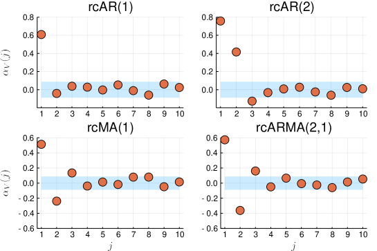
For the i.i.d. rcAR(1) the statistical procedure becomes very simple: just estimate $\alpha_{X}$ and check if it has a significant non-zero value only for $j=1$. This value is simply $\alpha_{X}(1)=\mathbb{E}\mathopen{}\mathclose{{}\left[\Phi_{k}}\right]$. For an illustration see figure 5. For higher order AR processes there are also exact equations linking the values of partial autocorrelation, covariance and coefficients of the model [30, 31].

Figure 5: Partial autocorrelation estimated from i.i.d. rcAR(1) with $\Phi_{k}\overset{d}{=}\mathcal{U}(0,1)$, rcAR(2) with $\Phi^{1}_{k}\overset{d}{=}\mathcal{U}(0,1),\Phi^{2}_{k}\overset{d}{=}\mathcal{U}(0,3/4)$, rcMA(1) with $\Theta_{k}\overset{d}{=}\mathcal{U}(0,2)$, and rcARMA(2,1) with $\Phi^{1}_{k}\overset{d}{=}\mathcal{U}(0,1)$, $\Phi^{2}_{k}\overset{d}{=}\mathcal{U}(-1/2,0)$, $\Theta_{k}\overset{d}{=}\mathcal{U}(0,2)$. Blue areas are 95% confidence intervals around 0. The memory function nicely fits the predictions, in particular one can easily distinguish the simplest rcAR(1) model. The choice of the presented rcARMA(2,1) was motivated by the Langevin equation (16). Here we used a 500 point trajectory—to observe only the characteristic rcAR(1) behaviour even shorter, 200-300 point trajectories are sufficient.

We now proceed to show that there actually is a way to detect differences between the dependence structure of ARMA and rcARMA. First, we estimate the mean rcAR(1) coefficient $\varphi=\mathbb{E}\mathopen{}\mathclose{{}\left[\Phi_{k}}\right]$, for instance, by using the partial autocorrelation. Next, the typical method of statistical verification for AR processes is to consider

$$\widetilde{Z}_{k}\mathrel{\mathop{:}}=V_{k}-\varphi V_{k-1}.$$ (42)

For the AR(1) with deterministic coefficient $\phi=\varphi$ this would be an estimate of the noise $Z_{k}$. Therefore, one could then use many of the testing methods if the series is i.i.d. However, for the rcAR(1),

$$\widetilde{Z}_{k}=(\Phi_{k}-\varphi)V_{k-1}+Z_{k}.$$ (43)

As $\mathbb{E}\mathopen{}\mathclose{{}\left[\Phi_{k}-\varphi}\right]=0$ the series is still uncorrelated, $\mathbb{E}[\widetilde{Z}_{k}\widetilde{Z}_{k+1}]=0$. It is a natural consequence of the applied procedure, which fits the system by removing the linear dependence. But the series $\widetilde{Z}_{k}$ remains non-linearly dependent. The value $\widetilde{Z}_{k}$ still depends on $V_{k-1}$ and consequently also on $\Phi_{k-1}$ appearing in the expression for $\widetilde{Z}_{k-1}$. This purely non-linear dependence can be detected only using non-linear measures of memory. The codifference function (see [77] for a detailed discussion) is one possible choice. It was proposed as a tool to study $\alpha$-stable variables, because it is finite even for variables with no second, or even lower, moments [78]—however its usefulness is by no means limited to this class. One of the few possible close definitions is the formula

$$\tau_{X}^{\theta}(j)\mathrel{\mathop{:}}=\frac{1}{\theta^{2}}\ln\frac{\mathbb{E}\mathopen{}\mathclose{{}\left[\rme^{\mathrm{i}\theta(X_{j}-X_{0})}}\right]}{\mathbb{E}\mathopen{}\mathclose{{}\left[\rme^{\mathrm{i}\theta X_{j}}}\right]\mathbb{E}\mathopen{}\mathclose{{}\left[\rme^{-\mathrm{i}\theta X_{0}}}\right]}.$$ (44)

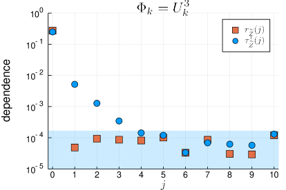
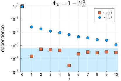
For any Gaussian process the codifference equals the covariance, so the difference between the two indicate any non-Gaussianity of the PDF and, what is important here, of the memory structure. For i.i.d. rcAR it can be expressed as a function of coefficients, and it can be analytically approximated, see (51) and the derivation below. As a simple example let us take the uniformly distributed $\Phi_{k}\overset{d}{=}\mathcal{U}(0,1)$ and $\Theta_{k}=\sqrt{D_{k}\Phi_{k}},D_{k}\overset{d}{=}\mathcal{U}(0,1)$. The covariance is zero as $\mathbb{E}[\widetilde{Z}_{k}\widetilde{Z}_{+1}]=0$, but the simulation yields $\tau_{\widetilde{Z}}^{1}(1)\approx 0.0023$, in good agreement with the analytic approximation is close $412/170535=0.0024$. Two more examples of rcAR(1) with higher dispersion of i.i.d. coefficients and even more prominent non-linear memory are shown in figure 6.

Figure 6: Comparison of the covariance and codifference for the series $\widetilde{Z}_{k}=V_{k}-\mathbb{E}\mathopen{}\mathclose{{}\left[\Phi_{k}}\right]V_{k-1}$ generated with two different i.i.d. $\Phi_{k}$ obtained from $U_{k}\overset{d}{=}\mathcal{U}(0,1)$ and $\Theta_{k}=\sqrt{\Phi_{k}}$. Blue areas are 95% confidence intervals around 0. The covariance is statistically zero for $j>0$, the codifference exhibits an exponential decay. We used two extremely long $10^{7}$-point trajectories in order to present a long range of $j$ and very weak dependence (statistically significant even around $10^{-3}$). Much shorter trajectories are sufficient for less extreme cases, the requirements in general are similar to those for the covariance estimation.

5.2 Non-Gaussianity

One possible approach of visualising the non-Gaussian behaviour of a diffusive process is to quantify the non-Gaussian nature of its dispersion in a manner similar to how we quantified non-Gaussian memory in the last section. We propose to use the non-linear measure of dispersion [77]

$$\zeta^{\theta}_{X}(j)\mathrel{\mathop{:}}=-\frac{2}{\theta^{2}}\ln\mathopen{}\mathclose{{}\left(\mathbb{E}\mathopen{}\mathclose{{}\left[\cos(\theta X_{j})}\right]}\right),$$ (45)

which is called log-characteristic function (LCF). It has the property that if the process is Gaussian it equals the MSD for any $\theta$. Therefore estimating it and plotting it together with the MSD reveals the non-Gaussian nature of the observed process. As the MSD averages over squares of the data, small values become even smaller and larger values become even more emphasised. Thus the MSD gives a large importance to the spread of extremal values. Conversely, for the LCF large values are translated into rapid oscillations of the cosine function and cancel each other, the LCF measures mainly the spread of the bulk.

For the classical case of non-Gaussian normal diffusion (4) the LCF is linear for small times, but logarithmic for large times, so it gets dominated by the linear MSD. This insight is more general. Random coefficient models discussed in this work can only describe diffusion processes with tails thicker than Gaussian. This means that compared to Gaussian diffusion with the same MSD more mass is located in the tails than in the bulk, and the LCF must be smaller than the MSD.

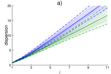
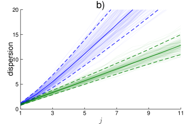
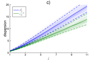
To use the LCF in practice one needs to fix the parameter $\theta$. For too small values the LCF converges to the MSD because $\cos(\theta x)\approx 1-\frac{1}{2}\theta^{2}x^{2}$, for too large values the estimation becomes challenging, because $\ln(0)$ diverges. In a typical case reasonable values are those for which $\theta\mathbb{E}\mathopen{}\mathclose{{}\left[|X(t)|}\right]\approx\pi$ so that $X(t)$ explores mainly the first period of the cosine function. In figure 7 we show a practical application of this technique performed using a relatively small sample of 500 integrated rcAR trajectories.

Figure 7: LCF and MSD calculated from 500 samples of the integrated rcAR processes. Semi-transparent lines are the individual estimated LCFs and MSDs, solid lines are the averaged ones, dashed lines denote $90\%$ confidence intervals. Case a) is $\Phi_{k}\overset{d}{=}\mathcal{U}(0,1),\Theta_{k}=\sqrt{\Phi_{k}}$; case b) is $\mathrm{P}(\Phi_{k}=0)=1/2=\mathrm{P}(\Phi_{k}=1),\Theta_{k}=\sqrt{\Phi_{k}}$; case c) is $\Phi_{k}=1/2,\Theta_{k}\overset{d}{=}1/2\times\mathcal{E}(1)$, where $\mathcal{E}$ is an exponential distribution. Cases a) and b) are based on variants of i.i.d. rcAR considered before, case c) is an example of a motion with varying diffusivity strongly concentrated at 0.

For rigorous statistical testing of the Gaussianity we propose to use the standard Jarque-Bera (JB) test [79]. It is a goodness of fit test of whether sample data have skewness and kurtosis that match a normal distribution. For the sample $\{x_{1},\ldots,x_{n}\}$ of observation the JB statistic is defined as

$$J=\frac{n}{6}\mathopen{}\mathclose{{}\left(\bar{s}^{2}+\frac{\bar{\kappa}^{2}}{4}}\right),$$ (46)

where $\bar{s}$ is the sample skewness and $\bar{\kappa}$ is the sample excess kurtosis. Samples from a normal distribution have an expected skewness of $0$ and an expected kurtosis of $3$ (excess kurtosis 0). Any deviation from this increases the JB statistic. The test is considered as standard and is implemented in various numerical packages, such as R tseries, Python SciPy.stats, Julia HypothesisTests, or Matlab.

This test is considered as one of the most powerful tests on normality but, if non-Gaussianity is detected, it does provide information on the origins of this behaviour. However, the idea of observing the kurtosis leads to an algorithm to distinguish between Gaussian and non-Gaussian (in particular, Lévy stable) distributions [80]. It is based on the empirical cumulative excess kurtosis (ECEK) which is defined as follows,

$$K(k)=\frac{\frac{1}{k}\sum_{i=1}^{k}(x_{i}-\bar{x})^{4}}{\mathopen{}\mathclose{{}\left(\frac{1}{k}\sum_{i=1}^{k}(x_{i}-\bar{x})^{2}}\right)^{2}}-3,$$ (47)

where $\bar{x}$ is an arithmetic mean of the random sample. This simple statistic serves as an indicator for whether there is a noticeable difference between Gaussian and non-Gaussian distributions. For the Gaussian case, for large numbers of observations it converges to the theoretical excess kurtosis 0, while for the non-Gaussian case the ECEK does not tend to 0 with increasing number $k$ of observations and, moreover, for distributions that do not have a finite forth moment it does not converge at all and behaves chaotically [80].

To distinguish between Gaussian and non-Gaussian distributions we also advocate the application of the discrimination algorithm based on examining the rate of convergence to the Gaussian law by means of the central limit theorem [81]. The idea of the algorithm is to analyse the convergence of the estimated index $\alpha$ of stability for sequential bootstrapped samples from the analysed data. If the estimated values converge to 2, then the data are light-tailed and belong to the domain of attraction of the Gaussian law. In particular, if the data are Gaussian, the estimated values should be equal to 2 for most of the cases. If the data belong to the domain of attraction of a non-Gaussian Lévy stable law, then the values should converge to a constant less than 2.

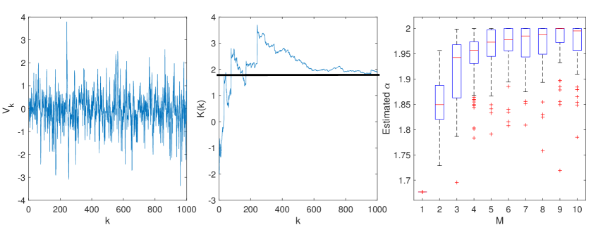
To illustrate the usefulness of the above statistical tools we consider an rcAR process for which the $\Phi_{k}$ are independent uniformly distributed on the interval $(0,0.95)$ and $\Theta_{k}=\sqrt{\Phi_{k}}$. In the left panel of figure 8 we can see a simulated trajectory of $V_{k}$ of length 1000 points. In the middle panel we display a plot of the ECEK for the simulated trajectory. We can see that the function converges to a constant close to 2 which clearly indicates a non-Gaussian behaviour and a finite positive excess kurtosis of the underlying distribution (a leptokurtic distribution). We also calculated analytically the exact value of the excess kurtosis (equations (28) and (50)) and obtained the value $1.83$, which coincides with the final values of the ECEK function. Finally, in the right panel of figure 8 we show the estimated values of the stability index $\alpha$, for different non-overlapping consecutive blocks of length $M$. For the first sample ($M=1$; corresponding to the whole trajectory), the value is significantly lower than 2, but for the other $M$ the values increase and tend to 2. This suggests that the simulated trajectory exhibits a non-Gaussian behaviour but its distribution belongs to the normal domain of attraction. The obtained results clearly suggest that the simulated trajectory exhibits a non-Gaussian behaviour and the underlying distribution is heavier-tailed than Gaussian (is leptokurtic) but belongs to the normal domain of attraction. The non-Gaussianity is also confirmed by the JB test which returns a $p$-value less than $0.001$.

Figure 8: Left: Trajectory of $V_{k}$ for which $\Phi_{k}\overset{d}{=}\mathcal{U}(0,0.95)$ and $\Theta_{k}=\sqrt{\Phi_{k}}$. Middle: Empirical cumulative excess kurtosis for the simulated trajectory. The solid black line represents the true kurtosis value which is equal to $1.83$. Right: Estimated values of the index of stability $\alpha$. The boxplots (for block lengths $M\in[1,10]$) constructed from 100 bootstrapped samples each of length 1000. The obtained results clearly suggest that the simulated trajectory exhibits a non-Gaussian behaviour and its distribution is leptokurtic but belongs to the normal domain of attraction.

5.3 Parameter estimation for rcAR processes

Finding reliable estimators of the parameters of the rcARMA models is a very important challenge. In this section we present preliminary ideas for some special cases of the models.

For an rcAR process with $\Phi$ being a simple function one can estimate its parameters either by extracting the constant periods of $\Phi$ and applying classical fitting techniques for the autoregressive processes to the extracted parts, or to consider a method which directly incorporates the information on switching between different autoregressive processes.

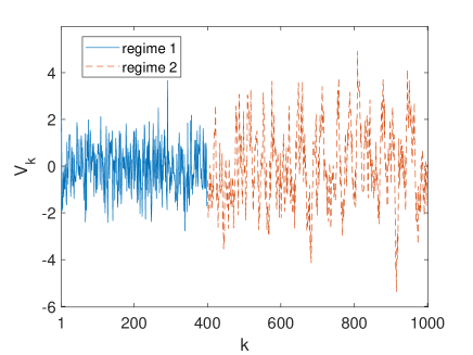
We now follow the latter idea and apply an algorithm based on hidden Markov Models (HMMs) [64, 82, 83]. This algorithm assumes that the trajectories switch among discrete diffusive states according to a stochastic (Markov) process. We consider a modification of the classical HMM, where the Markov regime switching is combined with AR$(1)$ processes [84]. To show the usefulness of this technique we take into account a two-regime parameter switching model, that is, a model with both regimes driven by AR$(1)$ processes with the autoregressive parameters $\phi_{1}$ and $\phi_{2}$. In figure 9 we present a simulated trajectory of $V_{k}$ of length 1000 for which $\Phi_{\alpha}$ changes from 0.2 to 0.8 at point 400. The estimated regime switching point is $399$ which is very close to the true value, and the estimated $\phi_{1}$ and $\phi_{2}$ coefficients are $0.17$, $0.79$ which confirms the usefulness of the procedure.

Figure 9: Two regimes identified by Hidden Markov Model methodology for a trajectory of $V_{k}$ for which $\Phi_{\alpha}$ changes from 0.2 to 0.8 at point 400. The estimated regime switching point is $399$ which is very close to the true value.

6 Discussion

As modern experiments such as single particle tracking routinely produce large amounts of data for the thermally and actively driven motion of test particles, the extraction of physical information from the garnered data becomes ever more important. On the one hand, this is met by the analysis of a growing number of complementary observables such as time averaged MSD [85, 86], higher order moments or mean maximal statistics [87], p-variation methods [88], first-passage methods [89], or single trajectory power spectra [8, 90]. On the other hand objective methods such as maximum likelihood approaches [91, 92, 93, 94] or machine learning [95] are being recognised as useful tools. Here the goal is to identify the physical model giving rise to the observed motion and estimate the involved parameters.

An alternative method, well established in financial market studies, is time series analysis. The latter seemingly does not share a lot with the physical approach of modelling. It puts the emphasis not on explaining the observed systems, but instead concentrates on fitting and prediction. Given a class of discrete linear filters suited to describe the general features of the data (for us the non-Gaussianity and linear MSD) it offers a wide choice of powerful methods for finding the optimal model and validating it. In other words by design it concentrates on the phenomenological description.

While a pure time series analysis approach initially may be discouraging for physically-minded researchers, the undeniable effectiveness of the time series methods make any connections to the framework of physics interesting and important. As noted in section 3 the correspondence between the Gaussian Langevin equation and the ARMA process is known (in fact, it was established as early as in 1959 [96]), but it never seemed to have gained a widespread appeal in the physical or biological physics community. Nevertheless, some recent progress was made, especially in topics related to the identification of fractional dynamics [63, 97] and accounting for the distortions made by measurement devices [71, 98].

This paper continues this line of research and aims at promoting to sample the best of both worlds. This is hard to achieve on a general level, but we study here important cases when a fruitful compromise can be made, and new information provided in the challenging analysis of non-Gaussian diffusion. Omitting the dynamics at time scales significantly shorter than what is available from observation (shorter than the sampling time $\Delta t$) leads to conceptually simple autoregressive models. These are straightforward and quick to simulate (using a medium class computer we were generating ten million values in under 2 seconds) and they provide a wide choice of statistical methods. Some of those, such as the partial autocorrelation, are intrinsically linked to discrete dynamics and have no continuous-time counterpart. Others, such as the kurtosis and codifference, profit from the analytic methods available for discrete variables.

In section 5 we illustrated important properties of the rcARMA processes and provided a list of statistical tools that can be useful in their identification and validation. In particular we showed that the codifference function can be used to distinguish between ARMA and rcARMA processes. To illustrate the non-Gaussianity of the rcARMA models we considered a non-linear measure of dispersion, namely the log-characteristic function and the empirical cumulative excess kurtosis, and studied the domain of attraction of the underlying distribution. Finally, we presented a hidden Markov model methodology which can be useful in fitting the process parameters. We also stress that the presented tools can be successfully applied for quite moderate lengths of the trajectories.

Our considerations are general and not limited to any particular system, as we discuss for related models based on random coefficient autoregression, which stem from a widely used form of the Langevin equation and reasonable models of heterogeneous environment. Thus, the provided methods are also universal. We hope that this study will promote the use of autoregressive models in modern data analysis, as well as prompt further studies into the physical meaning of these models.

Appendix A Appendix: Moments of $S$ and the approximation of codifference

Here we show the calculation of $\mathbb{E}\mathopen{}\mathclose{{}\left[S^{4}}\right]$ and the approximation of the codifference for an rcAR with i.i.d. coefficients. Starting with (27) we write

$$\mathbb{E}\mathopen{}\mathclose{{}\left[S^{4}}\right]=\mathbb{E}\mathopen{}\mathclose{{}\left[\mathopen{}\mathclose{{}\left(\Theta_{k}^{2}+\Phi_{k}^{2}\Theta_{k-1}^{2}+\Phi_{k}^{2}\Phi_{k-1}^{2}\Theta_{k-2}^{2}+\Phi_{k}^{2}\Phi_{k-1}^{2}\Phi_{k-1}^{2}\Theta_{k-3}^{2}+\ldots}\right)^{2}}\right].$$ (48)

We express this square as the sum of the elements squared plus twice the sum of each element multiplied by all elements to the right of it. The sum of squares is simply $\mathbb{E}\mathopen{}\mathclose{{}\left[\Theta_{k}^{4}}\right]/(1-\mathbb{E}\mathopen{}\mathclose{{}\left[\Phi_{k}^{4}}\right])$. As for the rest, in each element a factor of type $\mathbb{E}\mathopen{}\mathclose{{}\left[\Phi_{k-i}^{2}\Theta_{k-i}^{2}}\right]\mathbb{E}\mathopen{}\mathclose{{}\left[\Theta_{k-j}^{2}}\right]=\mathbb{E}\mathopen{}\mathclose{{}\left[\Phi_{k}^{2}\Theta_{k}^{2}}\right]\mathbb{E}\mathopen{}\mathclose{{}\left[\Theta_{k}^{2}}\right]$ appears. Note that it does not necessarily decouple, because in general $\Phi_{k}$ and $\Theta_{k}$ for fixed $k$ may be dependent. The remaining factor is

$$1 + \mathbb{E}\mathopen{}\mathclose{{}\left[\Phi_{k}^{2}}\right] + (\mathbb{E}\mathopen{}\mathclose{{}\left[\Phi_{k}^{2}}\right])^{2} + (\mathbb{E}\mathopen{}\mathclose{{}\left[\Phi_{k}^{2}}\right])^{3} + \ldots$$

$$\mathbb{E}\mathopen{}\mathclose{{}\left[\Phi_{k}^{4}}\right] + \mathbb{E}\mathopen{}\mathclose{{}\left[\Phi_{k}^{4}}\right]\mathbb{E}\mathopen{}\mathclose{{}\left[\Phi_{k}^{2}}\right] + \mathbb{E}\mathopen{}\mathclose{{}\left[\Phi_{k}^{4}}\right](\mathbb{E}\mathopen{}\mathclose{{}\left[\Phi_{k}^{2}}\right])^{2} + \mathbb{E}\mathopen{}\mathclose{{}\left[\Phi_{k}^{4}}\right](\mathbb{E}\mathopen{}\mathclose{{}\left[\Phi_{k}^{2}}\right])^{3} + \ldots$$

$$(\mathbb{E}\mathopen{}\mathclose{{}\left[\Phi_{k}^{4}}\right])^{2} + (\mathbb{E}\mathopen{}\mathclose{{}\left[\Phi_{k}^{4}}\right])^{2}\mathbb{E}\mathopen{}\mathclose{{}\left[\Phi_{k}^{2}}\right] + (\mathbb{E}\mathopen{}\mathclose{{}\left[\Phi_{k}^{4}}\right])^{2}(\mathbb{E}\mathopen{}\mathclose{{}\left[\Phi_{k}^{2}}\right])^{2} + (\mathbb{E}\mathopen{}\mathclose{{}\left[\Phi_{k}^{4}}\right])^{2}(\mathbb{E}\mathopen{}\mathclose{{}\left[\Phi_{k}^{2}}\right])^{3} + \ldots$$

$$(\mathbb{E}\mathopen{}\mathclose{{}\left[\Phi_{k}^{4}}\right])^{3} + (\mathbb{E}\mathopen{}\mathclose{{}\left[\Phi_{k}^{4}}\right])^{3}\mathbb{E}\mathopen{}\mathclose{{}\left[\Phi_{k}^{2}}\right] + (\mathbb{E}\mathopen{}\mathclose{{}\left[\Phi_{k}^{4}}\right])^{3}(\mathbb{E}\mathopen{}\mathclose{{}\left[\Phi_{k}^{2}}\right])^{2} + (\mathbb{E}\mathopen{}\mathclose{{}\left[\Phi_{k}^{4}}\right])^{3}(\mathbb{E}\mathopen{}\mathclose{{}\left[\Phi_{k}^{2}}\right])^{3} + \ldots$$

$$\quad\vdots$$ (49)

We recognise the product of two geometric series in the above. Finally, the fourth moment becomes

$$\mathbb{E}\mathopen{}\mathclose{{}\left[S^{4}}\right]=\frac{\mathbb{E}\mathopen{}\mathclose{{}\left[\Theta_{k}^{4}}\right]}{1-\mathbb{E}\mathopen{}\mathclose{{}\left[\Phi_{k}^{4}}\right]}+2\mathbb{E}\mathopen{}\mathclose{{}\left[\Phi_{k}^{2}\Theta_{k}^{2}}\right]\mathbb{E}\mathopen{}\mathclose{{}\left[\Theta_{k}^{2}}\right]\frac{1}{1-\mathbb{E}\mathopen{}\mathclose{{}\left[\Phi_{k}^{4}}\right]}\frac{1}{1-\mathbb{E}\mathopen{}\mathclose{{}\left[\Phi_{k}^{2}}\right]}.$$ (50)

Given these moments, one can easily calculate the kurtosis. It also makes it possible to obtain an analytic approximation of the codifference of the estimated noise $\widetilde{Z}_{k}\mathrel{\mathop{:}}=V_{k}-\varphi V_{k-1},\varphi=\mathbb{E}\mathopen{}\mathclose{{}\left[\Phi_{k}}\right]$. We show the procedure for $\tau_{\widetilde{Z}}^{\theta}(1)$. The method for other $\tau_{\widetilde{Z}}^{\theta}(j),j>1$ would be the same. We denote $\widetilde{\Phi}_{k}\mathrel{\mathop{:}}=\Phi_{k}-\varphi$ and start with a straightforward conditioning which yields

$$\tau_{\widetilde{Z}}^{\theta}(1)=\frac{1}{\theta^{2}}\ln\frac{\mathbb{E}\mathopen{}\mathclose{{}\left[\exp\mathopen{}\mathclose{{}\left(-\frac{\theta^{2}}{2}\mathopen{}\mathclose{{}\left((\widetilde{\Phi}_{k}\Phi_{k-1}-\widetilde{\Phi}_{k-1})^{2}S^{2}+(\widetilde{\Phi}_{k}-1)^{2}\Theta_{k-1}^{2}+\Theta_{k}^{2}}\right)}\right)}\right]}{\mathbb{E}\mathopen{}\mathclose{{}\left[\exp\mathopen{}\mathclose{{}\left(-\frac{\theta^{2}}{2}\mathopen{}\mathclose{{}\left(\widetilde{\Phi}_{k}^{2}S^{2}+\Theta_{k}^{2}}\right)}\right)}\right]^{2}},$$ (51)

where $S^{2}$ is assumed to have the distribution as in (27) and be independent from $\Phi_{k},\Theta_{k},\Phi_{k-1},\Theta_{k-1}$. Expanding the exponents in a Taylor series yields an approximation for the codifference which depends only on the moments of $\Phi_{k}$ and $\Theta_{k}$. Expansion up to first order, $\rme^{-x}\approx 1-x$, is equivalent to calculating the covariance, so it is zero. The second order, $\rme^{-x}\approx 1-x+x^{2}/2$ in general already provides quite good non-zero estimate. For the numerator it is

$$\approx 1-\frac{\theta^{2}}{2}\mathopen{}\mathclose{{}\left(\mathbb{E}\mathopen{}\mathclose{{}\left[\mathopen{}\mathclose{{}\left(\widetilde{\Phi}_{k}\Phi_{k-1}-\widetilde{\Phi}_{k-1}}\right)^{2}}\right]\mathbb{E}\mathopen{}\mathclose{{}\left[S^{2}}\right]+\mathbb{E}\mathopen{}\mathclose{{}\left[(\widetilde{\Phi}_{k}-1)^{2}\Theta^{2}_{k-1}+\Theta_{k}^{2}}\right]}\right)$$

$$+\frac{\theta^{4}}{8}\mathopen{}\mathclose{{}\left(\mathbb{E}\mathopen{}\mathclose{{}\left[\mathopen{}\mathclose{{}\left(\widetilde{\Phi}_{k}\Phi_{k-1}-\widetilde{\Phi}_{k-1}}\right)^{4}}\right]\mathbb{E}\mathopen{}\mathclose{{}\left[S^{4}}\right]}\right.$$

$$+2\mathbb{E}\mathopen{}\mathclose{{}\left[\mathopen{}\mathclose{{}\left(\widetilde{\Phi}_{k}\Phi_{k-1}-\widetilde{\Phi}_{k-1}}\right)^{2}\mathopen{}\mathclose{{}\left((\widetilde{\Phi}_{k}-1)^{2}\Theta^{2}_{k-1}+\Theta_{k}^{2}}\right)}\right]\mathbb{E}\mathopen{}\mathclose{{}\left[S^{2}}\right]$$

$$+\mathopen{}\mathclose{{}\left.\mathbb{E}\mathopen{}\mathclose{{}\left[\mathopen{}\mathclose{{}\left((\widetilde{\Phi}_{k}-1)^{2}\Theta^{2}_{k-1}+\Theta_{k}^{2}}\right)^{2}}\right]}\right).$$ (52)

The corresponding denominator is expanded into

$$\approx 1-{\theta^{2}}\mathopen{}\mathclose{{}\left(\mathbb{E}\big{[}\widetilde{\Phi}_{k}^{2}\big{]}\mathbb{E}\mathopen{}\mathclose{{}\left[S^{2}}\right]+\mathbb{E}[\Theta_{k}^{2}]}\right)+\frac{\theta^{4}}{4}\Bigg{(}\mathopen{}\mathclose{{}\left(\mathbb{E}\big{[}\widetilde{\Phi}_{k}^{2}\big{]}\mathbb{E}\mathopen{}\mathclose{{}\left[S^{2}}\right]+\mathbb{E}\mathopen{}\mathclose{{}\left[\Theta_{k}^{2}}\right]}\right)^{2}$$

$$+\mathopen{}\mathclose{{}\left(\mathbb{E}\big{[}\widetilde{\Phi}_{k}^{4}\big{]}\mathbb{E}\mathopen{}\mathclose{{}\left[S^{4}}\right]+2\mathbb{E}\big{[}\widetilde{\Phi}_{k}^{2}\Theta_{k}^{2}\big{]}\mathbb{E}\mathopen{}\mathclose{{}\left[S^{2}}\right]+\mathbb{E}\mathopen{}\mathclose{{}\left[\Theta^{4}_{k}}\right]}\right)\Bigg{)}.$$ (53)

The expected values that appear in this formulas are just linear combinations of the first four moments of $\Phi_{k},\Theta_{k}$ and their products. For variables generated as powers of a uniform distribution these are just integrals over polynomials. Also, without significant change the logarithm can be replaced by the fraction $\ln(x)\approx x-1$, which leads to a formula being a fraction of coefficient moments up to the fourth order.

References

- [1] T. Lucretius “De rerum natura. (On the Nature of the Universe)” (Oxford University Press, Oxford, UK, 2008).
- [2] R. Brown, “A brief account of microscopical observations made on the particles contained in the pollen of plants”, Phil. Mag. 4, 161 (1828).
- [3] A. Einstein, “Über die von der molekularkinetischen Theorie der Wärme geforderte Bewegung von in ruhenden Flüssigkeiten suspendierten Teilchen”, Ann. Physik (Leipzig) 322, 549 (1905).
- [4] W. Sutherland, “A dynamical theory of diffusion for non-electrolytes and the molecular mass of albumin”, Philos. Mag. 9, 781 (1905).
- [5] M. von Smoluchowski, “Zur kinetischen Theorie der Brownschen Molekularbewegung und der Suspensionen”, Ann. Phys. (Leipzig) 21, 756 (1906).
- [6] P. Langevin, “Sur la théorie de movement brownien [On the theory of Brownian motion]”, C. R. Acad. Sci. Paris 146, 530 (1908).
- [7] M. P. Norton and D. G. Karczub, “Fundamentals of noise and vibration analysis for engineers” (Cambridge University Press, Cambridge, UK, 2003).
- [8] D. Krapf, E. Marinari, R. Metzler, G. Oshanin, A. Squarcini, and X. Xu, “Power spectral density of a single Brownian trajectory: What one can and cannot learn from it”, New J. Phys. 20, 023029 (2018).
- [9] J.-P. Bouchaud and A. Georges, “Anomalous diffusion in disordered media: statistical mechanisms, models and physical applications”, Phys. Rep. 195, 127 (1990).
- [10] R. Metzler and J. Klafter, “The random walk’s guide to anomalous diffusion: a fractional dynamics approach”, Phys. Rep. 339, 1 (2000).
- [11] R. Metzler, J.-H. Jeon, A. G. Cherstvy, E. Barkai, “Anomalous diffusion models and their properties: non-stationarity, non-ergodicity, and ageing at the centenary of single particle tracking”, Phys. Chem. Chem. Phys. 16 24128 (2014).
- [12] I. Golding and E. C. Cox, “Physical nature of bacterial cytoplasm”, Phys. Rev. Lett. 96, 098102 (2006).
- [13] E. Kepten, A. Weron, I. Bronstein, K. Burnecki, and Y. Garini, “Uniform Contraction-Expansion Description of Relative Centromere and Telomere Motion”, Biophys. J. 109, 1454 (2015).
- [14] J.-H. Jeon, V. Tejedor, S. Burov, E. Barkai, C. Selhuber-Unkel, K. Berg-Sørensen, L. Oddershede, and R. Metzler, “In vivo anomalous diffusion and weak ergodicity breaking of lipid granules”, Phys. Rev. Lett. 106, 048103 (2011).
- [15] A. V. Weigel, B. Simon, M. M. Tamkun, and D. Krapf, “Ergodic and nonergodic processes coexist in the plasma membrane as observed by single-molecule tracking”, Proc. Nat. Acad. Sci. USA 108, 6438 (2011).
- [16] J.-H. Jeon, N. Leijnse, L. B. Oddershede, and R. Metzler, “Anomalous diffusion and power-law relaxation of the time averaged mean squared displacement in worm-like micellar solutions”, New J. Phys. 15, 045011 (2013).
- [17] J. Szymanski and M. Weiss, “Elucidating the origin of anomalous diffusion in crowded fluids”, Phys. Rev. Lett. 103, 038102 (2009).
- [18] A. Caspi, R. Granek, and M. Elbaum, “Enhanced diffusion in active intracellular transport”, Phys. Rev. Lett. 85, 5655 (2000).
- [19] J. F. Reverey, J.-H. Jeon, M. Leippe, R. Metzler, and C. Selhuber-Unkel, “Superdiffusion dominates intracellular particle motion in the supercrowded cytoplasm of pathogenic Acanthamoeba castellanii”, Sci. Rep. 5, 11690 (2015).
- [20] D. Robert, T. H. Nguyen, F. Gallet, and C. Wilhelm, “In vivo determination of fluctuating forces during endosome trafficking using a combination of active and passive microrheology”, PLoS ONE 4, e10046 (2010).
- [21] F. Höfling and T. Franosch, “Anomalous transport in the crowded world of biological cells”, Rep. Progr. Phys. 76, 046602 (2013).
- [22] K. Nørregaard, R. Metzler, C. Ritter, K. Berg-Sørensen, and L. Oddershede, “Manipulation and motion of organelles and single molecules in living cells”, Chem. Rev. 117, 4342 (2017).
- [23] B. Wang, S. M. Anthony, S. C. Bae, and S. Granick, “Anomalous yet Brownian”, Proc. Natl. Acad. Sci. U.S.A. 106, 15160 (2009).
- [24] B. Wang, J. Kuo, S. C. Bae, and S. Granick, “When Brownian diffusion is not Gaussian”, Nat. Mat. 11, 481 (2012).
- [25] S. Bhattacharya, D. Sharma, S. Saurabh, S. De, A. Sain, A. Nandi, and A. Chowdhury, “Plasticization of poly(vinylpyrrolidone) thin films under ambient humidity: Insight from single-molecule tracer diffusion dynamics”, J. Phys. Chem. B 117, 7771 (2013).
- [26] S. Hapca, J. W. Crawford, and I. M. Young, “Anomalous diffusion of heterogeneous populations characterized by normal diffusion at the individual level’, J. Roy. Soc. Interface 6, 111 (2009).
- [27] A. G. Cherstvy, O. Nagel, C. Beta, and R. Metzler,“Non-Gaussianity, population heterogeneity, and transient superdiffusion in the spreading dynamics of amoeboid cells”, Phys. Chem. Chem. Phys., 20, 23034 (2018).
- [28] A. Chechkin, F. Seno, R. Metzler, and I. Sokolov, “Brownian yet non-Gaussian diffusion: From superstatistics to subordination of diffusing diffusivities”, Phys. Rev. X 7, 021002 (2017).
- [29] R. S. Tsay, “Time series and forecasting: Brief history and future research”, J. Am. Stat. Assoc. 95, 638 (2000).
- [30] J. Box, G. Jenkins, and G. C. Reinsel, “Time Series Analysis: Forecasting and Control” (Wiley, New York, NY, 2008).
- [31] P. Brockwell and R. Davis, “Time Series: Theory and Methods”, (Springer-Verlag, Berlin, 2006).
- [32] T. J. Lampo, S. Stylianidou, M. P. Backlund, P. A. Wiggins, and A. J. Spakowitz, “Cytoplasmic RNA-protein particles exhibit non-Gaussian subdiffusive behavior”, Biophys. J. 112, 532 (2017).
- [33] J.-H. Jeon, M. Javanainen, H. Martinez-Seara, R. Metzler, and I. Vattulainen, “Protein crowding in lipid bilayers gives rise to non-Gaussian anomalous lateral diffusion of phospholipids and proteins”, Phys. Rev. X 6, 021006 (2016).
- [34] V. Sposini, A. V. Chechkin, F. Seno, G. Pagnini, and R. Metzler, “Random diffusivity from stochastic equations: comparison of two models for Brownian yet non-Gaussian diffusion”, New J. Phys. 20, 043044 (2018).
- [35] Y. Lanoiselée, N. Moutal, and D. S. Grebenkov, “Diffusion-limited reactions in dynamic heterogeneous media”, Nature Comm. 9, 4398 (2018).
- [36] R. Metzler, “Gaussianity fair: The riddle of anomalous yet non-Gaussian diffusion”, Biophys. J. 112 413 (2017).
- [37] W. He, H. Song, Y. Su, L. Geng, B. J. Ackerson, H. B. Peng, and P. Tong, “Dynamic heterogeneity and non-Gaussian statistics for acetylcholine receptors on live cell membrane”, Nature Comm. 7, 11701 (2016).
- [38] C. Beck and E. G. Cohen, “Superstatistics”, Physica A 322, 267 (2003).
- [39] C. Beck, “Superstatistical Brownian motion”, Prog. Theor. Phys. 162, 29 (2006).
- [40] C. Beck, “Generalized statistical mechanics for superstatistical systems”, Philos. Trans. Roy. Soc. A 369, 453 (2011).
- [41] H. Goldstein, "Multilevel Statistical Models" (Wiley, New York, NY, 2011).
- [42] B. G. Lindsay, “Mixture models: Theory, geometry and applications”, NSF-CBMS Reg. Conf. Ser. in Prob. Stat. 5 1 (1995).
- [43] J. Ślęzak, R. Metzler, and M. Magdziarz, “Superstatistical generalised Langevin equation: non-Gaussian viscoelastic anomalous diffusion”, New J. Phys. 20, 023026 (2018).
- [44] D. Tjøstheim, “Some doubly stochastic time series models”, J. Time Ser. Anal. 7, 51 (1986).
- [45] M. V. Chubynsky and G. W. Slater, “Diffusing diffusivity: A model for anomalous, yet Brownian, diffusion”, Phys. Rev. Lett. 113, 098302 (2014).
- [46] B. Øksendal, “Stochastic differential equations”, (Springer-Verlag, Berlin, 1995).
- [47] V. Tejedor and R. Metzler, “Anomalous diffusion in correlated continuous time random walks”, J. Phys. A 43, 082002 (2010).
- [48] M. Magdziarz, R. Metzler, W. Szczotka, and P. Zebrowski, “Correlated Continuous Time Random Walks in External Force Fields”, Phys. Rev. E 85, 051103 (2012).
- [49] J. Cox, J. Ingersoll, and S. Ross, “A theory of the term structure of interest rates”, Econometrica 53, 385 (1985).
- [50] A. Cherstvy and R. Metzler, “Anomalous diffusion in time-fluctuating non-stationary diffusivity landscapes”, Phys. Chem. Chem. Phys. 18, 23840 (2016).
- [51] R. Jain and K. Sebastian, “Diffusion in a crowded, rearranging environment”, J. Phys. Chem. B 120, 3988 (2016).
- [52] N. Tyagi and B. J. Cherayil, “Non-Gaussian Brownian Diffusion in Dynamically Disordered Thermal Environments”, J. Phys. Chem. B 121, 7204 (2017).
- [53] J. Beran, “Statistics for Long-Memory Processes”, (Chapman & Hall, New York, NY, 1994).
- [54] K. Burnecki and A. Weron, “Algorithms for testing of fractional dynamics: a practical guide to ARFIMA modelling”, J. Stat. Mech. 2014, P10036 (2014).
- [55] K. Burnecki, G. Sikora, and A. Weron, “Fractional process as a unified model for subdiffusive dynamics in experimental data”, Phys. Rev. E 86, 041912 (2012).
- [56] P. S. Kokoszka and M. S. Taqqu, “Infinite variance stable ARMA processes”, J. Time Ser. Anal. 15, 203 (1994).
- [57] P. S. Kokoszka and M. S. Taqqu, “Fractional ARIMA with stable innovations”, Stoch. Proc. Appl. 60, 19 (1995).
- [58] R. F. Engle, “Autoregressive conditional heteroscedasticity with estimates of the variance of United Kingdom inflation”, Econometrica 50, 987 (1982).
- [59] T. Bollerslev, “Generalized autoregressive conditional heteroskedasticity”, J. Econom. 31, 307 (1986).
- [60] T. Breusch and A. Pagan, “A simple test for heteroscedasticity and random coefficient variation”, Econometrica 47, 1287 (1979).
- [61] D. B. Nelson, “Conditional heteroskedasticity in asset returns: A new approach”, Econometrica 59, 347 (1991).
- [62] R. T. Baillie, C.-F. Chung, and M. A. Tieslau, “Analysing inflation by the fractionally integrated ARFIMA-GARCH model”, J. Appl. Econ. 11, 23 (1996).
- [63] M. Balcerek, H. Loch-Olszewska, J. A. Torreno-Pina, M. F. García-Parajo, A. Weron, C. Manzo, and K. Burnecki, “Inhomogeneous membrane receptor diffusion explained by a fractional heteroscedastic time series model”, Phys. Chem. Chem. Phys. 21, 3114 (2019).
- [64] A. A. Stanislavsky, A. Weron, J. Janczura, K. Niczyj, and K. Burnecki, “Solar X-ray variability in terms of a fractional heteroskedastic time series model”, Mon. Notices Royal Astron. Soc. 2019.
- [65] D. Nicholls and B. Quinn, “Random Coefficient Autoregressive Models: An Introduction” (Lecture Notes in Statistics, Springer, New York, NY, 2012).
- [66] S. R. Sugata and B. Sankha, “Rate of convergence to normality of estimators in a random coefficient ARMA(p,q) model”, Commun. Stat. Theory Meth. 40, 1081 (2011).
- [67] R. Zwanzig “Nonequlibrium Statistical Mechanics” (Oxford University Press, Oxford, UK, 2001).
- [68] W. T. Coffey, Y. P. Kalmykov, and J. T. Waldron, “The Langevin Equation” (Word Scientific, Singapore, 1996).
- [69] P. Brockwell, R. Davis, and Y. Yang, “Continuous-time Gaussian autoregression”, Stat. Sinica 17, 63 (2007).
- [70] J. Ślęzak and A. Weron, “From physical linear systems to discrete-time series. A guide for analysis of the sampled experimental data”, Phys. Rev. E 91, 053302 (2015).
- [71] S. Drobczyński and J. Ślęzak, “Time-series methods in analysis of the optical tweezers recordings”, Appl. Opt. 54, 7106 (2015).
- [72] D. Ernst, J Köhler, and M. Weiss, “Probing the type of anomalous diffusion with single-particle tracking”, Phys. Chem. Chem. Phys. 16, 7686 (2014).
- [73] Y. Lanoiselée and D. S. Grebenkov, “A model of non-Gaussian diffusion in heterogeneous media”, J. Phys. A 51, 145602 (2018).
- [74] M. R. Evans and S. N. Majumdar, “Diffusion with stochastic resetting”, Phys. Rev. Lett. 106, 160601 (2011).
- [75] S. Kotz, T. J. Kozubowski, and K. Podgórski, “The Laplace Distribution and Generalizations” (Birkhäuser, Boston, MA, 2001).
- [76] Y. Liang, A. Thavaneswaran, and N. Ravishanker, “RCA models: Joint prediction of mean and volatility”, Stat. & Prob. Lett. 83, 527 (2013).
- [77] J. Ślęzak, R. Metzler, and M. Magdziarz, “Codifference can detect ergodicity breaking and non-Gaussianity”, New J. Phys. 21, 053008 (2019).
- [78] G. Samorodnitsky and M. Taqqu, “Stable Non-Gaussian Random Processes” (Chapman & Hall, London, 1994).
- [79] C. M. Jarque and A. K. Bera, “A test for normality of observations and regression residuals”, Int. Stat. Rev. 55, 163 (1987).
- [80] K. Burnecki, A. Wyłomańska, A. Beletskii, V. Gonchar, and A. Chechkin, “Recognition of stable distribution with Lévy index close to 2”, Phys. Rev. E 85, 056711 (2012).
- [81] K. Burnecki, A. Wyłomańska, and A. Chechkin, “Discriminating between light-and heavy-tailed distributions with limit theorem”, PLoS ONE 10, e0145604 (2015).
- [82] L. E. Baum and T. Petrie, “Statistical inference for probabilistic functions of finite state markov chains”, Ann. Math. Statist. 37, 1554 (1966).
- [83] T. Sungkaworn, M.-L. Jobin, K. Burnecki, A. Weron, M. J. Lohse, and D. Calebiro, “Single-molecule imaging reveals receptor-G protein interactions at cell surface hot spots”, Nature 550, 543 (2017).
- [84] J. Janczura and R. Weron, “Efficient estimation of Markov regime-switching models: An application to electricity spot prices”, AStA Advances in Statistical Analysis 96, 385 (2012).
- [85] Y. He, S. Burov, R. Metzler, and E. Barkai, “Random Time-Scale Invariant Diffusion and Transport Coefficients”, Phys. Rev. Lett. 101, 058101 (2008).
- [86] J. H. P. Schulz, E. Barkai, and R. Metzler, “Aging renewal theory and application to random walks”, Phys. Rev. X 4, 011028 (2014).
- [87] V. Tejedor, O. Bénichou, R. Voituriez, R. Jungmann, F. Simmel, C. Selhuber-Unkel, L. Oddershede, and R. Metzler, “Quantitative analysis of single particle trajectories: Mean maximal excursion method”, Biophys. J. 98, 1364 (2010).
- [88] M. Magdziarz, A. Weron, K. Burnecki, and J. Klafter, “Fractional Brownian Motion Versus the Continuous-Time Random Walk: A Simple Test for Subdiffusive Dynamics”, Phys. Rev. Lett. 103, 180602 (2009).
- [89] S. Condamin, V. Tejedor, R. Voituriez, O. Bénichou, and J. Klafter, “Probing microscopic origins of confined subdiffusion by first-passage observables”, Proc. Natl. Acad. Sci. USA 105, 5675 (2008).
- [90] D. Krapf, N. Lukat, E. Marinari, R. Metzler, G. Oshanin, C. Selhuber-Unkel, A. Squarcini, L. Stadler, M. Weiss, and X. Xu, “Spectral Content of a Single Non-Brownian Trajectory”, Phys. Rev. X 9, 011019 (2019).
- [91] F. Persson, M. Linden, C. Unoson, and J. Elf, “Extracting intracellular diffusive states and transition rates from single-molecule tracking data”, Nature Meth. 10, 265 (2013).
- [92] M. A. Lomholt and J. Krog, “Bayesian inference with information content model check for Langevin equation”, Phys. Rev. E 96, 062106 (2017).
- [93] S. Thapa, M. A. Lomholt, J. Krog, A. G. Cherstvy, and R. Metzler, “Bayesian nested sampling analysis of single particle tracking data: maximum likelihood model selection applied to stochastic diffusivity data”, Phys. Chem. Chem. Phys. 20, 29018 (2018).
- [94] A. G. Cherstvy, S. Thapa, C. E. Wagner, and R. Metzler, “Non-Gaussian, non-ergodic, and non-Fickian diffusion of tracers in mucin hydrogels”, Soft Matter 15, 2526 (2019).
- [95] G. Muñoz-Gil, M. A. Garcia-March, C. Manzo, J. D. Martín-Guerrero, and M. Lewenstein, “Machine learning method for single trajectory characterization”, E-print arXiv:1903.02850.
- [96] A. W. Phillips, “The estimation of parameters in systems of stochastic differential equations”, Biometrika 46, 67 (1959).
- [97] K. Burnecki, G. Sikora, A. Weron, M. M. Tamkun, and D. Krapf, “Identifying diffusive motions in single-particle trajectories on the plasma membrane via fractional time-series models”, Phys. Rev. E 99, 012101 (2019).
- [98] G. Sikora, E. Kepten, A. Weron, M. Balcerek, and K. Burnecki, “An efficient algorithm for extracting the magnitude of the measurement error for fractional dynamics”, Phys. Chem. Chem. Phys. 19, 26566 (2017).