Optimal gauge for the multimode Rabi model in circuit QED

Abstract

In circuit QED, a Rabi model can be derived by truncating the Hilbert space of the anharmonic qubit coupled to a linear, reactive environment. This truncation breaks the gauge invariance present in the full Hamiltonian. We analyze the determination of an optimal gauge such that the differences between the truncated and the full Hamiltonian are minimized. Here, we derive a simple criterion for the optimal gauge. We find that it is determined by the ratio of the anharmonicity of the qubit to an averaged environmental frequency. We demonstrate that the usual choices of flux and charge gauge are not necessarily the preferred options in the case of multiple resonator modes.

Circuit QED Blais et al. (2004); Wallraff et al. (2004) is a central subject of quantum information science that has deepened our understanding of light-matter interaction Schmidt and Koch (2013); Devoret and Schoelkopf (2013); Wendin (2017). Most implementations consist of a two-level system (qubit) that is coupled to a linear environment. The qubit is formed by the two lowest energy levels of an anharmonic multilevel-system. For the physics of interest only the qubit subspace is important. The Schrieffer-Wolff (SW) transformation Schrieffer and Wolff (1966); Bravyi et al. (2011) is the standard method to perturbatively derive an effective Hamiltonian description within this subspace. For most purposes, it is sufficient to consider the effective Hamiltonian only to first order, yielding the well known quantum Rabi model (QRM). However, since the Hamiltonian of the non-truncated system is unique only up to a unitary transformation, the effective description is gauge dependent to every finite order Lamb (1952); Yang (1976). This gauge ambiguity becomes particularly important in the (ultra) strong coupling regime. It has been found that the QRM derived in a gauge where the qubit-resonator coupling is mediated by the flux variables leads to different predictions than the one where the coupling is mediated by the charge variables De Bernardis et al. (2018a, b); Di Stefano et al. (2018).

In this work, we look at the issue from a different perspective. We use the gauge degree of freedom to find an optimal gauge such that the results of the effective model are as close as possible to full model. Importantly, we take account of the need for a multimode description Nigg et al. (2012); Solgun et al. (2014); Parra-Rodriguez et al. (2018); Hassler et al. (2019) in the quest for achieving the ultra-strong coupling regime Gely et al. (2017); Bosman et al. (2017); Manucharyan et al. (2017); Frisk Kockum et al. (2019). To increase the flexibility, we not only consider the extremal cases of purely flux or charge mediated coupling but perform a general gauge transformation that smoothly interpolates between the two. A similar transformation has been used in Stokes and Nazir (2019) to extend the Jaynes-Cummings model into the ultra-strong coupling regime.

We find that already the second order term of the effective Hamiltonian within the SW method is a good indicator of the validity of the QRM. Based on this observation, we derive a simple analytical criterion for the optimal gauge and benchmark it against numerical simulations of the full problem.

Figure 1: (a) Circuit diagram of a qubit with potential $U(\phi_{\rm q})$, capacitance $C_{\rm q}$, and inductance $L_{\rm q}$ that is coupled to a general reactive environment. In the Forster form, the latter is represented by $N$ resonators with capacitances $C_{k}$ and inductances $L_{k}$ ($k=1,\dots,N$). (b) Fluxonium qubit (consisting of a Josephson junction with energy $E_{\text{J}}$ in parallel to the capacitance $C_{\rm q}$ and a large inductance $L_{\rm q}$), capacitively coupled to two resonators with inductances $L_{r_{k}}$ and capacitances $C_{r_{k}}$ ($k=1,2$). In the text, the example of a single resonator (dashed box) is treated separately.

For a qubit coupled to a single-mode resonator, the flux gauge is always the best gauge De Bernardis et al. (2018a, b); Manucharyan et al. (2017). This serves as an analogue of the dipole gauge in quantum optics Cohen‐Tannoudji et al. (1999). Considering more than one mode drastically changes this simple picture. The optimal gauge may now deviate from the pure flux gauge as can be demonstrated with two resonator modes. We show that this already has implications for weak to moderate coupling.

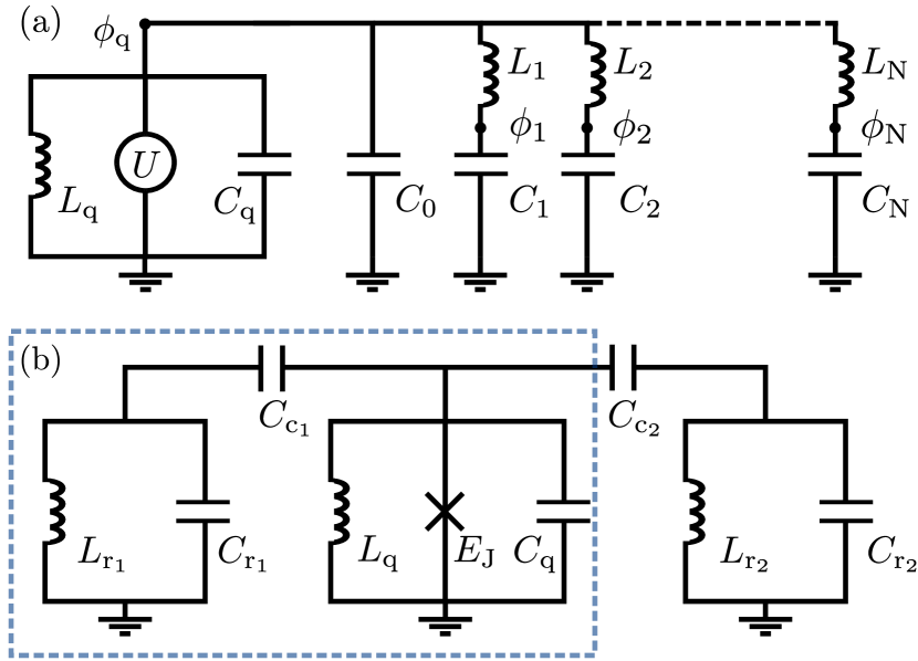
General case.—Consider a qubit consisting of an LC-oscillator in parallel with a symmetric potential $U(\phi_{\rm q})$ that is coupled to a linear, reactive environment, cf. Fig. 1(a). We denote the qubit Hamiltonian $H_{\rm q}$ and the resonator Hamiltonian $H_{\rm r}$. They are coupled via the interaction $V$ such that the total Hamiltonian is given by $H=H_{\rm q}+H_{\rm r}+V$. Using the unitary freedom of the Hamiltonian formalism, we introduce a gauge parameter $\eta\in[0,1]$ that linearly interpolates between a qubit-resonator interaction mediated by the flux variables $\phi_{k}$ (for $\eta=0$) and the charge variables $Q_{k}$ (for $\eta=1$) Sup . We will refer to these extremal cases as the flux and the charge gauge, respectively. For a general gauge, the interaction reads

$$V(\eta) =-\sum_{k=1}^{N}\left[\frac{(1-\eta)\phi_{\rm q}\phi_{k}}{L_{k}}+\frac{\eta\,Q_{\rm q}Q_{k}}{C_{\Sigma}}\right]$$ (1)

$$\quad\quad\quad+(1-\eta)^{2}\sum_{k=1}^{N}\frac{\phi_{\rm q}^{2}}{2L_{k}}+\eta^{2}\frac{\Bigl{(}\sum_{k=1}^{N}Q_{k}\Bigr{)}^{2}}{2C_{\Sigma}}\,;$$

here, $C_{\Sigma}=C_{\rm q}+C_{0}$ denotes the total capacitance of the qubit to ground. The first term of Eq. (1) is the analogue of the paramagnetic coupling. The second part is a diamagnetic term that renormalizes qubit and the resonator frequencies and ensures the gauge invariance of the full Hamiltonian Sup ; Malekakhlagh and Türeci (2016).

For most quantum information applications, we are interested in projecting $H_{\rm q}$ onto a subspace $S=\{\ket{0},\ket{1}\}$ spanned by the two lowest eigenstates. To obtain an effective Hamiltonian, we apply the SW method resulting in $H_{\rm eff}=\sum_{j=0}^{K}H_{j}$ to $K$-th order. The first order result $H_{0}+H_{1}$ corresponds to the projection of $H$ onto $S$. It is equivalent to the generalized QRM Sup ; not

$$H_{\rm QRM}(\eta)=-\frac{\hbar\omega_{10}^{\rm q}}{2}\sigma^{z}+\sum_{k=1}^{N}\hbar\omega_{k}a_{k}^{\dagger}a_{k}$$ (2)

$$\quad\quad+\hbar\sum_{k=1}^{N}\Bigl{[}(1-\eta)g_{k}^{\phi}\sigma^{x}(a_{k}+a^{\dagger}_{k})+\eta g^{Q}_{k}\sigma^{y}(a_{k}-a_{k}^{\dagger})\Bigr{]}\,,$$

where $\hbar\omega_{nm}^{\rm q}$ is the energy difference between the $n$-th and the $m$-th eigenstate of $H_{\rm q}$ and $\sigma^{j}$ ($j=x,y,z$) denote the Pauli operators. In Eq. (2), we have rewritten the variables of the $k$-th resonator mode with frequency $\omega_{k}$ in terms of bosonic creation operators $a^{\dagger}_{k}$ and annihilation operators $a_{k}$. The coupling between the qubit and the $k$-th resonator mode is given by $g_{k}^{\phi}=\matrixelement{1}{\phi_{\rm q}}{0}\sqrt{Z_{k}/2\hbar L_{k}^{2}}$ and $g_{k}^{Q}=\matrixelement{1}{Q_{\rm q}}{0}/\sqrt{2\hbar Z_{k}C_{\Sigma}^{2}}$, where $Z_{k}$ is the characteristic impedance of the $k$-th mode. In deriving Eq. (2), we neglected the diamagnetic shift due to the second term present in Eq. (1) for simplicity. For weak coupling, the diamagnetic shift is irrelevant. In general, it can be accounted for using symplectic diagonalization Idel et al. (2016); Simon et al. (1999).

Restricting the perturbative series of $H_{\rm eff}$ to any finite order necessarily results in a gauge dependent model. The source of the gauge dependence of the QRM is that the coupling between the subspace $S$ and its orthogonal complement $S^{\bot}$ is not properly taken into account in the projection. Increasing the order $K$ weakens the gauge dependence Cederbaum et al. (1989); Aharonov and Au (1979) at the expense of introducing a dressed basis that results in a model that strays quite far from the natural interpretation of the QRM. In this respect, the lowest order approximation provided by the QRM is an appealing model as it yields a low-energy description without rotating the basis. In the simple effective model Eq. (2), choosing a gauge such that the QRM accurately captures the physics of the full Hamiltonian is crucial. We are thus concerned with the task of finding an optimal gauge parameter $\eta_{*}$ such that the differences between the QRM and the full Hamiltonian are minimized.

A criterion for the optimal gauge.—To address this issue, we note that the validity of the QRM is directly proportional to the coupling strength between $S$ and $S^{\bot}$. The higher order SW terms $H_{j}$ ($j>1$) can therefore be used as an estimator for the difference between the full model and its effective description as a QRM. Based on this observation, we derive an analytic criterion for the optimal gauge.

In particular, we focus on the second order term $H_{2}$, which will provide the largest corrections to $H_{\rm QRM}$ for weak coupling. $H_{2}$ is proportional to matrix elements $V_{nm}=\matrixelement{n}{V}{m}$ of the interaction, where $\ket{n}\in S$ and $\ket{m}\in S^{\bot}$. Motivated by Eq. (1), we define the paramagnetic flux coupling operator $G^{\phi}_{k}=\phi_{{\rm q}}\phi_{k}^{\rm zp}/\hbar L_{k}$ and the charge coupling operator $G^{Q}_{k}=Q_{\rm q}Q_{k}^{\rm zp}/\hbar C_{\Sigma}$ cou . Here, we have approximated the resonator matrix elements by their zero point fluctuations $\phi_{k}^{\rm zp}\simeq\sqrt{\hbar Z_{k}}$ and $Q_{k}^{\rm zp}\simeq\sqrt{\hbar/Z_{k}}$, respectively. In order to estimate the relevance of the flux versus the charge coupling (for the transition $m\mapsto n$), we introduce the ratio $f_{nm}=\bigl{[}\sum_{k}(G^{\phi}_{k})_{nm}\bigr{]}/\bigl{[}\sum_{k}(G^{Q}_{k})_{nm}\bigr{]}$. Using the fact that $(Q_{{\rm q}})_{nm}=i\omega_{nm}^{\rm q}C_{\Sigma}(\phi_{{\rm q}})_{nm}$, it can be compactly rewritten as

$$\absolutevalue{f_{nm}}=\frac{\sum_{k}p_{k}\omega_{k}}{\omega^{\rm q}_{nm}}=\frac{\bar{\omega}}{\omega^{\rm q}_{nm}}\,,$$ (3)

where $\bar{\omega}$ is the average of the resonator frequencies $\omega_{k}$ with the weights $p_{k}=Z_{k}^{-1/2}/\bigl{(}\sum_{l}Z_{l}^{-1/2}\bigr{)}$.

The interpretation of Eq. (3) is as follows: if $\absolutevalue{f_{nm}}\ll 1$, the coupling between $S$ and $S^{\bot}$ in the flux gauge is much smaller than the coupling in the charge gauge. The QRM with $\eta\approx 0$ is therefore a good approximation of the full model, making the flux gauge the preferred choice. But, if $\absolutevalue{f_{nm}}\gg 1$, the coupling of the qubit subspace to higher levels is small in the charge gauge which thus is the optimal gauge. In the intermediate regime, where $\absolutevalue{f_{nm}}\simeq 1$, both, flux and charge variables contribute similarly to the coupling between $S$ and $S^{\bot}$. Consequently, we expect the optimal gauge to be neither the pure charge nor the flux gauge but a mixed gauge with $\eta\neq 0,1$.

For weak qubit-resonator interactions, the dominant contribution to $H_{2}$ will be due to the coupling of the first and second excited level of the qubit. The character of the coupling of the optimal gauge is therefore mostly determined by the ratio of the anharmonicity of the qubit to an effective frequency of the linear environment. We conclude that $f_{21}$ of Eq. (3) provides a simple estimation of the optimal coupling. It requires only knowledge of the qubit anharmonicity and the frequency and impedances of the linear environment. We illustrate these findings with two specific examples in the following.

Single resonator.—First, we consider a qubit coupled to a single resonator ($N=1$). Note that in this case the average frequency $\bar{\omega}$ in Eq. (3) is equal to $\omega_{1}$. For the interaction between the qubit and the resonator mode to be appreciable, we assume that $\omega_{1}\simeq\omega^{\rm q}_{\rm 10}$. Consequently, Eq. (3) yields $\absolutevalue{f_{21}}\simeq\omega^{\rm q}_{10}/\omega^{\rm q}_{21}$ and the optimal gauge is solely determined by the properties of the qubit. To reach strong coupling, the qubit has to be anharmonic with $\omega_{10}^{\rm q}\ll\omega_{\rm 21}^{\rm q}$ Manucharyan et al. (2017). This implies $\absolutevalue{f_{21}}\ll 1$, so we find that the flux gauge is always the optimal gauge for this case.

To demonstrate this result, we numerically study the fluxonium qubit with $E_{\rm L}=(\phi_{0}/2\pi)^{2}/L_{\rm q}\lesssim E_{\rm J}$ and $U(\phi_{\rm q})=-E_{\rm J}\cos[2\pi(\phi_{\rm q}-\phi_{\rm ext})/\phi_{0}]$ Manucharyan et al. (2009);

Figure 2: Spectrum of the full Hamiltonian $H$ (solid lines) and the Rabi model Hamiltonian $H_{\rm QRM}$ (dashed lines) for a fluxonium qubit coupled to a single resonator (a) and to two resonators (b). The qubit parameters are $(E_{\rm J},E_{C},E_{L})=\hbar(12.5,3.75,0.5)\,\rm GHz$, where $E_{C}=e^{2}/2C_{\Sigma}$ and $E_{\rm L}=(\phi_{0}/2\pi)^{2}/L_{\rm q}$. The resulting qubit frequency is $\omega_{\rm 10}^{\rm q}=0.5\,\rm GHz$ and $\omega_{21}^{\rm q}=13\,\rm GHz$. Furthermore, $\omega_{1}=\omega_{10}^{q}$ and $g^{\phi}_{1}/\omega_{1}=0.07$. In (b) the parameters of the second resonator are $C_{\rm r_{2}}=C_{\rm r_{1}}$, $C_{\rm c_{2}}=C_{\rm c_{1}}$ and $\omega_{2}\approx\omega_{12}^{\rm q}$ such that $\bar{\omega}=10.7\,\rm GHz$. The value $\eta_{*}$ that minimizes $\lVert H_{2}\rVert_{*}$ is shown as a vertical dashed line.

here, $E_{\rm J}$ is the Josephson energy, $\phi_{0}=h/2e$ is the superconducting flux quantum, and $\phi_{\rm ext}$ is an external magnetic flux threading the superconducting loop. We set the external flux to the degeneracy point $\phi_{\rm ext}=\tfrac{1}{2}\phi_{0}$ which results in a symmetric potential. The qubit parameters are chosen such that the qubit is strongly anharmonic with $\omega_{21}^{\rm q}/\omega^{\rm q}_{\rm 10}\approx 25$ (see Fig. 2 for details). The fluxonium qubit is coupled to a parallel combination of a capacitor $C_{\rm r_{1}}$ and inductance $L_{\rm r_{1}}$ which together form a resonator with a frequency $\omega_{1}=\omega_{10}^{\rm q}$, cf. Fig. 1(b) (dashed box). The setup can be mapped to the canonical Foster circuit with $N=1$ shown in Fig. 1(a) Sup .

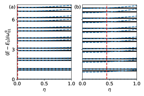
Figure 2(a) shows the spectrum of the full Hamiltonian (solid) compared to the spectrum of $H_{\rm QRM}$ (dotted) as a function of $\eta$. The spectra agree well in the flux gauge ($\eta=0$). For increasing values of $\eta$, that is for more charge-like gauges, the spectral agreement between truncated and full model decreases. The disagreement is more pronounced in levels with higher energy as they are closer to the energy of the second excited level of the qubit. We observe that $f_{21}$ of Eq. (3) is suitable for estimating the overall tendency for being charge or flux-like. A more quantitative estimate of the optimal coupling $\eta_{*}$ can be obtained by calculating the norm of $H_{2}$. Based on the discussion surrounding Eq. (3), we expect that $\eta_{*}$ is approximately the $\eta$ for which the norm $\lVert H_{2}\rVert_{*}$ Nor is minimized. For the parameters in Fig. 2(a), the minimum of $\lVert H_{2}\rVert_{*}$ is at $\eta=0$, which is shown in red (dotted) and agrees well with the visual impression conveyed by the spectrum. A quantitative analysis can be found in Ref. Sup .

Two resonators.— As a second example, we treat the case where there are two relevant modes ($N=2$). As before, the first mode is close to resonance with the qubit frequency. The second mode with frequency $\omega_{2}$ can be interpreted as a parasitic mode. Since the average frequency $\bar{\omega}$ in Eq. (3) is a function of all modes coupled to the qubit, the optimal gauge is now also dependent on the parasitic mode. This is true even for strongly off-resonant modes, as the coupling to higher modes in the flux gauge increases $\propto(\omega_{2})^{2}$ at fixed impedance, see Eq. (1). As a result, for large detuning with $\omega_{2}\gg\omega_{21}^{\rm q}$, the charge gauge becomes more favorable. In contrast to the single-mode case, the optimal gauge for two resonators is not determined by the properties of the qubit alone but depends on the parameters of the whole circuit.

To show this effect, we perform numerical simulations of the circuit in Fig. 1(b). The fluxonium is capacitively coupled to two parallel LC oscillators via the capacitances $C_{\rm c_{1}}$ and $C_{\rm c_{2}}$. This circuit can be mapped to the canonical Foster circuit depicted in Fig. 1(a) Sup . Figure 2(b) shows the spectrum of the full Hamiltonian (black, solid) and the QRM (dashed, blue) as a function of $\eta$. The parameters of the qubit and the first resonator are the same as in Fig. 2(a). The frequency of the second resonator, however, is significantly larger such that $\bar{\omega}\approx\omega_{12}^{\rm q}$. In contrast to the single-resonator case, the spectral lines of $H$ and $H_{\rm QRM}$ do not cross at $\eta\approx 0$ but rather around $\eta\approx 0.5$, suggesting the optimal gauge does not coincide with the usual ad-hoc choices of the flux or charge gauge. This is in agreement with the prediction based on the minimization of $\lVert H_{2}\rVert_{*}$ which yields $\eta_{*}=0.45$ (shown as a dashed vertical line).

The deviation between $H$ and $H_{\rm QRM}$ is state dependent for finite qubit anharmonicities, a fact that we have neglected so far. As a result, the intersection of the spectral lines of $H$ and $H_{\rm QRM}$ in Fig. 2(b) is shifted towards smaller values of $\eta$ for increasing energy of the levels. In the intermediate regime where $\omega_{\rm q}^{21}\simeq\bar{\omega}$ ($f_{21}\simeq 1$), the optimal gauge is thus always a compromise which minimizes the differences of $H$ and $H_{\rm QRM}$ in the relevant spectral range.

To demonstrate the dependence of the optimal gauge on $\bar{\omega}$, we keep the frequency $\omega_{1}$ of the first mode in resonance with the qubit while varying $\bar{\omega}$. To simulate an experimentally feasible scenario, we choose the inductance $L_{r_{2}}$ of the second resonator as the parameter that we vary Castellanos-Beltran et al. (2008). Decreasing $L_{\rm r_{2}}$ while keeping all other parameters constant increases the frequency $\omega_{2}$ of the parasitic mode while simultaneously decreasing its impedance. Since $\bar{\omega}$ decreases with the square root of $Z_{2}$ but increases linearly with $\omega_{2}$, the average frequency $\bar{\omega}$ grows with decreasing $L_{r_{2}}$. To quantify the agreement between the full Hamiltonian and the QRM, we use the standard deviation $\sigma=\bigl{[}\sum_{i=0}^{M}(E_{i}-e_{i})^{2}/M\bigr{]}^{1/2}$ between the energies $E_{i}$ of the full Hamiltonian and the energies $e_{i}$ of the QRM (measured from the respective ground-state energy). We denote the value of $\eta$ for which $\sigma$ is minimized by $\eta_{\sigma}$.

Figure 3: (a) Deviation $\sigma$ of the energy eigenvalues of the full model from the energy eigenvalues of the QRM as function of $\eta$ and $\bar{\omega}$. The qubit parameters and the parameters of the first resonator are the same as in Fig. 2. The coupling capacitances to both resonators are equal $C_{c_{1}}=C_{c_{2}}=C_{c}$. The average frequency $\bar{\omega}$ is varied by changing the inductance of the second resonator $L_{\rm r_{2}}$. The value $\eta_{\sigma}$ for which $\sigma$ is minimized is shown in as a solid line. The value of $\eta_{*}$ for which $\lVert H_{2}\rVert_{*}$ is minimized is shown as a dashed line. (b) Coupling strength between qubit levels $n$ and $m$ (see legend) as a function of $\bar{\omega}$.

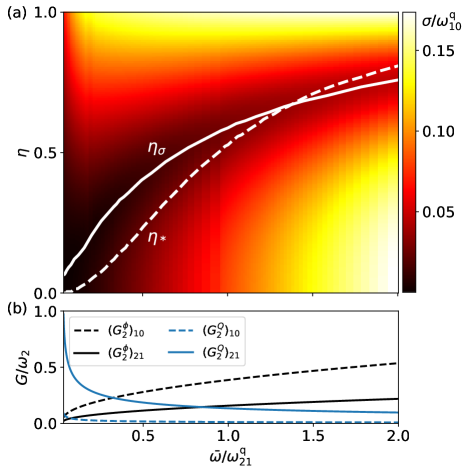
Figure 3(a) shows $\sigma$ as a function of $\bar{\omega}$ and $\eta$ for the first 15 energy levels. We see that $\eta_{\sigma}\approx 0$ (flux gauge) for $\bar{\omega}\ll\omega_{10}^{\rm q}$. Increasing the average frequency $\bar{\omega}$, the optimal gauge moves towards the charge gauge. Furthermore, we note that although the minimal value of $\sigma$ increases with increasing $\bar{\omega}$, the overall deviation between the full model and the QRM at $\eta_{\sigma}$ is only a few percent. The value $\eta_{*}$ which minimizes $\lVert H_{2}\rVert_{*}$ is shown as a dashed line. It can be observed that $\eta_{*}$ behaves similarly to $\eta_{\sigma}$.

To support our discussion surrounding Eq. (3), we analyze the coupling between $S$ and $S^{\bot}$. Figure 3(b) shows $(G^{\phi}_{2})_{nm}$ (black) and $(G^{Q}_{2})_{nm}$ (blue) for the parameters of Fig. 3(a). In general, the charge coupling $G^{Q}$ decreases while the flux coupling $G^{\phi}$ increases with increasing $\bar{\omega}$. For small values of $\bar{\omega}$, the dominant quantity is $(G^{Q}_{2})_{21}$. This results in a large coupling between $S$ and $S^{\bot}$ in the charge gauge, making the flux gauge the preferred choice. As $\bar{\omega}$ increases, the coupling to the higher qubit levels in the charge variables decreases and eventually becomes comparable to the coupling in the flux variables, making the choice of the optimal gauge less trivial.

Conclusion.— We have analyzed the gauge dependence of the effective description of an anharmonic system coupled to a general linear environment. Using a SW transformation, we have derived a simple, analytic criterion that predicts the optimal gauge where the physics of the non-truncated Hamiltonian is accurately captured by the QRM. We have demonstrated that the optimal gauge for a qubit resonantly coupled to a single resonator is completely determined by the qubit parameters and is in the flux-like regime for strongly anharmonic qubits. We have seen that coupling a qubit to more than one mode can result in an optimal gauge that is neither the charge nor the flux gauge but a non-trivial combination of the two. This is especially relevant with the increasing interest in the ultra-strong coupling regime which raises the need for multimode descriptions.

Supplement

I Gauge transformation

In this chapter, we introduce the gauge transformation discussed in the main text on a Lagrangian level. The Lagrangian $\mathcal{L}(\boldsymbol{\phi},\dot{\boldsymbol{\phi}})$ of a qubit in potential $U$ coupled to a general linear environment is a function of the fluxes $\boldsymbol{\phi}=\left(\phi_{\rm q},\phi_{1},\dots,\phi_{\rm N}\right)^{T}$ and the voltages proportional to $\dot{\boldsymbol{\phi}}$. Here, the dot denotes the time derivative. Using the capacitance matrix $C$ and the inverse of the inductance matrix $M=L^{-1}$, it can be written as

$$\mathcal{L}(\boldsymbol{\phi},\dot{\boldsymbol{\phi}})=\frac{1}{2}\dot{\boldsymbol{\phi}}^{T}C\dot{\boldsymbol{\phi}}-\frac{1}{2}\boldsymbol{\phi}^{T}M\boldsymbol{\phi}-U(\phi_{\rm q})\,.$$ (S1)

The Euler-Lagrange equations are invariant under coordinate transformations. The choice of coordinates corresponds to choosing a specific gauge in electromagnetic field theory. In Eq. (S1), the flux variable $\phi_{\rm q}$ is distinguished from the rest by the presence of the potential $U(\phi_{\rm q})$. We thus consider coordinate transformations $\phi=T\phi^{\prime}$ that preserve this structure and leave the variable $\phi_{\rm q}$ invariant. In its most general form, such a transformation is given by

$$T=\begin{pmatrix}1&{\bf 0}\\ \bf{t}&R\end{pmatrix}\,,$$ (S2)

where $R$ is an invertible matrix and $\bf{t}$ is an $N$-dimensional vector.

In general, both $C$ and $M$ provide a qubit-resonator coupling. In the following, we show that it is not possible to decouple the qubit from the resonator with a transformation of the form of Eq. (S2). To demonstrate this, we write $C$ and $M$ in the same block structure as Eq. (S2)

$$C=\begin{pmatrix}\kappa&{\bf c}^{T}\\ \bf{c}&C_{\rm r}\end{pmatrix}\,,\quad M=\begin{pmatrix}\mu&{\bf m}^{T}\\ \bf{m}&M_{\rm r}\end{pmatrix}\,.$$ (S3)

Here, $\kappa$ is the qubit capacitance and $\mu$ is the qubit inductance. Moreover, $C_{\rm r}$ and $M_{\rm r}$ are the capacitance and inverse inductance matrices of the resonators. The vectors $\bf{c}$ and $\bf{m}$ couple the flux and voltage variables of the qubit and the resonators. Under the transformation Eq. (S2), $C$ and $M$ transform as $C^{\prime}=T^{T}CT$ and $M^{\prime}=T^{T}MT$ which yields the transformed off-diagonal blocks ${\bf c^{\prime}}=R{\bf c}+RC_{\rm r}{\bf t}$ and ${\bf m^{\prime}}=R{\bf m}+RM_{\rm r}{\bf t}$. Therefore, in order for ${\bf c^{\prime}}$ and ${\bf m^{\prime}}$ to vanish at the same time, the following equations have to be satisfied

$${\bf m}-M_{\rm r}C_{\rm r}^{-1}{\bf c} =0\,,$$ (S4)

$${\bf c}-C_{\rm r}M^{-1}_{\rm r}{\bf m} =0\,.$$ (S5)

These equations can only be satisfied simultaneously if the qubit and the resonators are uncoupled. Nevertheless, one can choose coordinates such that the qubit is coupled to the resonator only through the capacitance or the inverse inductance matrix, respectively. In the following, we fix ${\bf t}$ and introduce a gauge parameter $\eta$ that linearly interpolates between these two extreme cases

$${\bf t}=-\left[(1-\eta)C_{\rm r}^{-1}{\bf c}+\eta M_{\rm r}^{-1}{\bf m}\right]\,.$$ (S6)

One can easily verify that $\eta=0$ results in a block-diagonal capacitance matrix $C^{\prime}$. The coupling is then completely inductive and we call the corresponding gauge flux gauge. On the other hand, $\eta=1$ block-diagonalizes $M^{\prime}$ which results in a purely capacitive coupling. We call the corresponding gauge charge gauge.

II Full Hamiltonian

Figure 1(a) in the main text shows a qubit in a potential $U$ coupled to a general admittance modelled by a series of LC oscillators. Choosing the flux gauge to represent the circuit (determined by the choice of ground node Devoret (1995)), the Lagrangian is given by

$$\mathcal{L}(\boldsymbol{\phi},\dot{\boldsymbol{\phi}})=\frac{C_{\Sigma}\dot{\phi}_{\rm q}^{2}}{2}-\frac{\phi_{\rm q}^{2}}{2L_{\rm q}}-U(\phi_{\rm q})+\sum_{k=1}^{N}\left[\frac{C_{k}\dot{\phi}_{k}^{2}}{2}-\frac{\left(\phi_{k}-\phi_{\rm q}\right)^{2}}{2L_{k}}\right]\,.$$ (S7)

Here, $C_{\Sigma}=C_{\rm q}+C_{0}$ is the total capacitance of the qubit to ground. We introduce a gauge parameter $\eta$ by performing the variable transformation Eq. (S2) discussed in the previous section. We use the specific ${\bf t}$ from Eq. (S6). For the Lagrangian in Eq. (S7) the coupling vectors read ${\bf c}={\bf 0}$ and ${\bf m}=(-L^{-1}_{1},-L^{-1}_{2},\dots,-L^{-1}_{\rm N})^{T}$. The capacitance and inductance matrices of the resonators are diagonal. They are given by $C_{\rm r}=\text{diag}(C_{1},C_{2},\dots,C_{\rm N})$ and $M_{\rm r}=\text{diag}(L^{-1}_{1},L^{-1}_{2},\dots,L^{-1}_{\rm N})$. Performing the transformation yields

$$\mathcal{L}^{\prime}(\boldsymbol{\phi}^{\prime},\dot{\boldsymbol{\phi}}^{\prime})=\frac{C_{\Sigma}\dot{\phi}_{\rm q}^{\prime 2}}{2}-\frac{\phi_{\rm q}^{\prime 2}}{2L_{\rm q}}-U(\phi_{\rm q}^{\prime})+\sum_{k=1}^{N}\left[\frac{C_{k}\left(\dot{\phi}_{k}^{\prime}+\eta\dot{\phi}_{\rm q}^{\prime}\right)^{2}}{2}-\frac{\left(\phi_{k}^{\prime}-\left(1-\eta\right)\phi_{\rm q}^{\prime}\right)^{2}}{2L_{k}}\right]\,,$$ (S8)

where, $\boldsymbol{\phi}=T\boldsymbol{\phi}^{\prime}$. We define the conjugate momenta $Q_{i}^{\prime}=\partialderivative{\mathcal{L^{\prime}}}{\phi_{i}^{\prime}}$ of the flux variables $\boldsymbol{\phi}^{\prime}$, and perform a Legendre transformation which yields the Hamiltonian $H=\sum_{i}Q^{\prime}_{i}\dot{\phi}^{\prime}_{i}-\mathcal{L^{\prime}}$. To obtain a quantum mechanical description, we promote the canonical variables to operators $\phi^{\prime}_{i}\rightarrow\hat{\phi}_{i}$ and $Q_{i}^{\prime}\rightarrow\hat{Q}_{i}$, and impose the canonical commutation relation $\commutator{\hat{\phi}_{i}}{\hat{Q}_{j}}=i\hbar\delta_{ij}$, where $\delta_{ij}$ is the Kronecker delta. The total Hamiltonian $H(\eta)=H_{\rm q}+H_{\rm r}+V(\eta)$ can then be split into a qubit Hamiltonian $H_{\rm q}$, a resonator Hamiltonian $H_{\rm r}$ and the interaction $V$ with

$$H_{\rm q} =\frac{\hat{Q}_{\rm q}^{2}}{2C_{\Sigma}}+\frac{\hat{\phi}_{\rm q}^{2}}{2L_{\rm q}}+U(\hat{\phi}_{\rm q})\,,\qquad H_{\rm r}=\sum_{k=1}^{N}\frac{\hat{Q}_{k}^{2}}{2C_{k}}+\frac{\hat{\phi}_{k}^{2}}{2L_{k}}\,,$$ (S9a)

$$V(\eta) =-\sum_{k=1}^{N}\left[\frac{(1-\eta)\hat{\phi}_{\rm q}\hat{\phi}_{k}}{L_{k}}+\frac{\eta\hat{Q}_{\rm q}\hat{Q}_{k}}{C_{\Sigma}}\right]+(1-\eta)^{2}\sum_{k=1}^{N}\frac{\hat{\phi}_{\rm q}^{2}}{2L_{k}}+\eta^{2}\frac{\left(\sum_{k=1}^{N}\hat{Q}_{k}\right)^{2}}{2C_{\Sigma}}\,.$$ (S9b)

The interaction $V$ in Eq. (S9b) is given in Eq. (1) of the main text where the hats over the operators have been omitted. Note that the Hamiltonian $H(\eta)$ is related to the Hamiltonian $H(\eta^{\prime})$ through the unitary transformation $R=\exp[-i(\eta^{\prime}-\eta)\hat{\phi}_{\rm q}\sum_{k}\hat{Q}_{k}/\hbar]$ such that $R^{\dagger}H(\eta)R=H(\eta^{\prime})$. The difference of $H(\eta)-H(0)$ corresponds to a pseudopertubation of Ref. Aharonov and Au (1979).

III Schrieffer-Wolff transformation

In this section, we perform a SW transformation to derive the QRM Eq. (2). Similar to the main text, we define the low energy subspace of the qubit $S=\left\{\ket{0},\ket{1}\right\}$ and its orthogonal complement $S^{\bot}$. Furthermore, we define the projector $P=\outerproduct{0}{0}+\outerproduct{1}{1}$ onto $S$. The projector onto $S^{\bot}$ is then given by $Q=1-P$. The coupling between the subspaces $S$ and $S^{\bot}$ is provided by $PVQ$. Performing a SW transformation to block-diagonalize $H$ with respect to $S$ and $S^{\bot}$ results in an effective Hamiltonian $H_{\rm eff}=\sum_{j=0}^{K}H_{j}$ Winkler (2003). The zeroth order is given by the projection of the uncoupled Hamiltonian onto $S$

$$H_{0}=PH_{\rm q}P+H_{\rm r}=-\hbar\frac{\omega_{10}^{\rm q}}{2}\sigma^{z}+\hbar\sum_{k=1}^{N}\omega_{k}a^{\dagger}_{k}a_{k}\,.$$ (S10)

Here, $\hbar\omega_{10}^{\rm q}$ is the energy difference between the ground state and the first excited state of the qubit. Furthermore, we have defined the frequencies $\omega_{k}=1/\sqrt{L_{k}C_{k}}$ and the bosonic raising and lowering operators of the $k$-th mode

$$\hat{\phi}_{n} =\sqrt{\frac{\hbar Z_{k}}{2}}\left(a^{\dagger}_{k}+a_{k}\right)\,,$$ (S11)

$$\hat{Q}_{k} =i\sqrt{\frac{\hbar}{2Z_{k}}}\left(a^{\dagger}_{k}-a_{k}\right)\,,$$ (S12)

where $Z_{k}=\sqrt{L_{k}/C_{k}}$ is the characteristic impedance of the $k$-th mode. The next order is given by the projection of the interaction $V$ onto $S$

$$H_{1}=PV(\eta)P=\hbar\sum_{k=1}^{N}\Bigl{[}(1-\eta)g_{k}^{\phi}\sigma^{x}(a_{k}+a^{\dagger}_{k})+\eta g^{Q}_{k}\sigma^{y}(a_{k}-a_{k}^{\dagger})\Bigr{]}-\frac{\left(1-\eta\right)\alpha}{2}\sigma^{z}-\frac{\eta^{2}\hbar}{2C_{\Sigma}}\left(\sum_{k=1}^{N}\frac{a^{\dagger}_{k}-a_{k}}{\sqrt{Z_{k}}}\right)^{2}\,,$$ (S13)

where $g_{k}^{\phi}=\matrixelement{1}{\phi_{\rm q}}{0}\sqrt{Z_{k}/2\hbar L_{k}^{2}}$ and $g_{k}^{Q}=\matrixelement{1}{Q_{\rm q}}{0}/\sqrt{2\hbar Z_{k}C_{\Sigma}^{2}}$. Furthermore, $\alpha=(\matrixelement{1}{\phi_{\rm q}^{2}}{1}-\matrixelement{0}{\phi_{\rm q}^{2}}{0})\sum_{n}1/L_{n}$. The last two terms in Eq. (S13) are diamagnetic renormalizations of the qubit and resonator frequencies. If these terms are omitted, the first order effective Hamiltonian $H_{0}+H_{1}$ is equal to the QRM Eq. (2) in the main text. For weak qubit-resonator coupling this is a reasonable assumption.

IV Foster Representation

The circuit shown in Fig. 1(b) can be mapped onto the general Foster form of Fig. 1(a). Assuming a symmetric coupling $C_{c_{1}}=C_{c_{2}}=C_{c}$, the capacitances and inductances are given by the following substitutions

$$C_{k}=\frac{C_{c}^{2}}{C_{c}+C_{r_{k}}}\,\qquad L_{k}=\frac{L_{r_{k}}(C_{c}+C_{r_{i}})^{2}}{C_{c}^{2}}\,,$$ (S14)

with

$$C_{0}=\frac{C_{c}C_{r_{1}}}{C_{c}+C_{1}}\,,$$ (S15)

for the one-mode setup (dashed box) and

$$C_{0}=C_{c}\left(\frac{C_{r_{1}}}{C_{c}+C_{r_{1}}}+\frac{C_{r_{2}}}{C_{c}+C_{r_{2}}}\right)\,,$$ (S16)

for the two-mode setup.

V Single Resonator results, detailed

Figure S1: Standard deviation $\sigma$ of the full spectrum and the effective Hamiltonian $H_{\rm eff}$ to $K$-th order. The QRM corresponds to $K=1$ (blue). Moreover $K=2$ (red), $K=3$ (green) and the exact SW transformed Hamiltonian $K=\infty$ (purple) are shown. Additionally, the norm $\lVert H_{2}\rVert_{*}$ of the first perturbative correction to $H_{\rm QRM}$ is shown (black, dashed). The parameters are the same as in Fig. 2 in the main text.

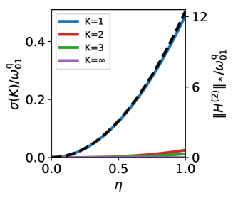
In this section, we show supporting data for one qubit coupled to one resonator. Figure S1 shows the standard deviation $\sigma(K)=\sqrt{(1/M)\sum_{i=0}^{M}(E_{i}-e_{i}(K))^{2}}$ for the first $15$ states. Note that here $e_{i}(K)$ denote the eigenvalues of the SW transformed Hamiltonian $H_{\rm eff}$ to $K$-th order. In Fig. S1, the parameters are the same as in Fig. 2 in the main text. For all finite values of $K$, the minimum of $\sigma$ is at $\eta\approx 0$ demonstrating that the flux gauge is optimal in this case.

Furthermore, we see that adding higher order terms to the Rabi Hamiltonian mitigates the effect of the broken gauge invariance. The deviation between full and effective model becomes less sensitive to variations in $\eta$ with increasing order in the SW method. The exact SW transformation Cederbaum et al. (1989) (purple) results in a gauge invariant two-level description. Additionally, the norm of $H_{2}$ is shown(black, dashed). We observe a non-linear increase towards charge-like gauges as expected from the previous discussion. For $K=1$ (blue, solid), we see a strikingly similar functional dependence on $\eta$ as in $\lVert{H_{2}}\rVert_{*}$, indicating that a large part of the corrections to $H_{\rm QRM}$ are already captured by $H_{2}$.

References

- Blais et al. (2004) Alexandre Blais, Ren-Shou Huang, Andreas Wallraff, S. M. Girvin, and R. J. Schoelkopf, “Cavity quantum electrodynamics for superconducting electrical circuits: An architecture for quantum computation,” Phys. Rev. A 69, 062320 (2004).
- Wallraff et al. (2004) A Wallraff, D I Schuster, A Blais, L Frunzio, R.-S Huang, J Majer, S Kumar, S M Girvin, and R J Schoelkopf, “Strong coupling of a single photon to a superconducting qubit using circuit quantum electrodynamics,” Nature 431 (2004).
- Schmidt and Koch (2013) Sebastian Schmidt and Jens Koch, “Circuit qed lattices: Towards quantum simulation with superconducting circuits,” Ann. Phys. 525, 395–412 (2013).
- Devoret and Schoelkopf (2013) M. H. Devoret and R. J. Schoelkopf, “Superconducting circuits for quantum information: An outlook,” Science 339, 1169–1174 (2013).
- Wendin (2017) G Wendin, “Quantum information processing with superconducting circuits: a review,” Rep. Prog. Phys. 80, 106001 (2017).
- Schrieffer and Wolff (1966) J. R. Schrieffer and P. A. Wolff, “Relation between the anderson and kondo hamiltonians,” Phys. Rev. 149, 491–492 (1966).
- Bravyi et al. (2011) Sergey Bravyi, David P. DiVincenzo, and Daniel Loss, “Schrieffer–wolff transformation for quantum many-body systems,” Ann. Phys. 326, 2793 – 2826 (2011).
- Lamb (1952) Willis E. Lamb, “Fine structure of the hydrogen atom. iii,” Phys. Rev. 85, 259–276 (1952).
- Yang (1976) Kuo-Ho Yang, “Gauge transformations and quantum mechanics i. gauge invariant interpretation of quantum mechanics,” Ann. Phys. 101, 62 – 96 (1976).
- De Bernardis et al. (2018a) Daniele De Bernardis, Philipp Pilar, Tuomas Jaako, Simone De Liberato, and Peter Rabl, “Breakdown of gauge invariance in ultrastrong-coupling cavity qed,” Phys. Rev. A 98, 053819 (2018a).
- De Bernardis et al. (2018b) Daniele De Bernardis, Tuomas Jaako, and Peter Rabl, “Cavity quantum electrodynamics in the nonperturbative regime,” Phys. Rev. A 97, 043820 (2018b).
- Di Stefano et al. (2018) O. Di Stefano, A. Settineri, V. Macrì, L. Garziano, R. Stassi, S. Savasta, and F. Nori, “Resolution of gauge ambiguities in ultrastrong-coupling cavity qed,” arXiv:1809.08749 (2018).
- Nigg et al. (2012) Simon E. Nigg, Hanhee Paik, Brian Vlastakis, Gerhard Kirchmair, S. Shankar, Luigi Frunzio, M. H. Devoret, R. J. Schoelkopf, and S. M. Girvin, “Black-box superconducting circuit quantization,” Phys. Rev. Lett. 108, 240502 (2012).
- Solgun et al. (2014) Firat Solgun, David W. Abraham, and David P. DiVincenzo, “Blackbox quantization of superconducting circuits using exact impedance synthesis,” Phys. Rev. B 90, 134504 (2014).
- Parra-Rodriguez et al. (2018) A Parra-Rodriguez, E Rico, E Solano, and I L Egusquiza, “Quantum networks in divergence-free circuit QED,” Quantum Sci. Technol. 3, 024012 (2018).
- Hassler et al. (2019) Fabian Hassler, Jakob Stubenrauch, and Alessandro Ciani, “Equation of motion approach to black-box quantization: Taming the multimode jaynes-cummings model,” Phys. Rev. B 99, 014515 (2019).
- Gely et al. (2017) Mario F. Gely, Adrian Parra-Rodriguez, Daniel Bothner, Ya. M. Blanter, Sal J. Bosman, Enrique Solano, and Gary A. Steele, “Convergence of the multimode quantum rabi model of circuit quantum electrodynamics,” Phys. Rev. B 95, 245115 (2017).
- Bosman et al. (2017) Sal J Bosman, Mario F Gely, Vibhor Singh, Alessandro Bruno, Daniel Bothner, and Gary A Steele, “Multi-mode ultra-strong coupling in circuit quantum electrodynamics,” npj Quantum Inf. 3, 46 (2017).
- Manucharyan et al. (2017) Vladimir E Manucharyan, Alexandre Baksic, and Cristiano Ciuti, “Resilience of the quantum rabi model in circuit QED,” J. Phys. A 50, 294001 (2017).
- Frisk Kockum et al. (2019) Anton Frisk Kockum, Adam Miranowicz, Simone De Liberato, Salvatore Savasta, and Franco Nori, “Ultrastrong coupling between light and matter,” Nat. Rev. Phys. 1, 19–40 (2019).
- Stokes and Nazir (2019) Adam Stokes and Ahsan Nazir, “Gauge ambiguities imply Jaynes-Cummings physics remains valid in ultrastrong coupling QED,” Nat. Comm. 10, 499 (2019).
- Cohen‐Tannoudji et al. (1999) Claude Cohen‐Tannoudji, Jacques Dupont‐Roc, and Gilbert Grynberg, Photons and Atoms (Wiley-VCH, Weinheim, 1999).
- (23) See supplementary material for details on the gauge transformation, the full Hamiltonian, the SWT, and additional numerics for the one-mode case.
- Malekakhlagh and Türeci (2016) Moein Malekakhlagh and Hakan E. Türeci, “Origin and implications of an -like contribution in the quantization of circuit-qed systems,” Phys. Rev. A 93, 012120 (2016).
- (25) Here, the parity symmetry is important for giving the selection rules .
- Idel et al. (2016) Martin Idel, Sebatian Soto Gaona, and Michael M. Wolf, “Perturbation Bounds for Williamson’s Symplectic Normal Form,” arXiv:1609.01338 (2016).
- Simon et al. (1999) R. Simon, S. Chaturvedi, and V. Srinivasan, “Congruences and canonical forms for a positive matrix: Application to the schweinler–wigner extremum principle,” J. Math. Phys. 40, 3632–3642 (1999).
- Cederbaum et al. (1989) L S Cederbaum, J Schirmer, and H D Meyer, “Block diagonalisation of hermitian matrices,” J. Phys. A 22, 2427–2439 (1989).
- Aharonov and Au (1979) Y. Aharonov and C. K. Au, “Gauge invariance and pseudoperturbations,” Phys. Rev. A 20, 1553–1562 (1979).
- (30) Note that the couplings and are generalizations of the couplings introduced in Eq. (2) such that and .
- Manucharyan et al. (2009) Vladimir E. Manucharyan, Jens Koch, Leonid I. Glazman, and Michel H. Devoret, “Fluxonium: Single cooper-pair circuit free of charge offsets,” Science 326, 113–116 (2009).
- (32) In Figs. 2 and 3 we have used the trace norm for an Hermitian operator with eigenvalues . Since we are only interested in the value of that minimizes the norm of , other norms can be used as well.
- Castellanos-Beltran et al. (2008) M A Castellanos-Beltran, K D Irwin, G C Hilton, L R Vale, and K W Lehnert, Nat. Phys. 4, 929 (2008).
- Devoret (1995) M.H. Devoret, “Quantum fluctuations in electrical circuits,” in Proceedings of the Les Houches Summer School, Session LXIII (Elsevier Science B. V, New York, 1995).
- Winkler (2003) Roland Winkler, Spin-Orbit Coupling Effects in Two-Dimensional Electron and Hole System (Springer Berlin Heidelberg, 2003) pp. 201–205.