Spot evolution on LQ Hya during 2006–2017: temperature maps based on SOFIN and FIES data
Abstract
Context. LQ Hya is one of the most frequently studied young solar analogue stars. Recently, it has been observed to show intriguing behaviour by analysing long-term photometry: during 2003–2009, a coherent spot structure migrating in the rotational frame has been reported by various authors, but since that time the star has entered a chaotic state where coherent structures seem to have disappeared and rapid phase jumps of the photometric minima occur irregularly over time.
Aims. LQ Hya is one of the stars included in the SOFIN/FIES long-term monitoring campaign extending over 25 years. Here we publish new temperature maps for the star during 2006–2017, covering the chaotic state of the star.
Methods. We use a Doppler imaging technique to derive surface temperature maps from high-resolution spectra.
Results. From the mean temperatures of the Doppler maps we see a weak but systematic increase in the surface temperature of the star. This is consistent with the simultaneously increasing photometric magnitude. During nearly all observing seasons we see a high-latitude spot structure which is clearly nonaxisymmetric. The phase behaviour of this structure is very chaotic but agrees reasonably well with the photometry. Equatorial spots are also frequently seen, but many of them we interpret to be artefacts due to the poor to moderate phase coverage.
Conclusions. Even during the chaotic phase of the star, the spot topology has remained very similar to the higher activity epochs with more coherent and long-lived spot structures: we see high-latitude and equatorial spot activity, the mid latitude range still being most often void of spots. We interpret the erratic jumps and drifts in phase of the photometric minima to be caused by changes in the high-latitude spot structure rather than the equatorial spots.
Key Words.:
stars: activity – stars: imaging – starspots1 Introduction
LQ Hya (HD 82558, GL 355) is a rapidly rotating single K2V star in the thin disk population (Fekel et al., 1986; Montes et al., 2001; Hinkel et al., 2017). LQ Hya has an estimated mass of (Kovári et al., 2004; Tetzlaff et al., 2011), an effective temperature of about 5000 K (Donati, 1999; Kovári et al., 2004; Hinkel et al., 2017), an estimated age from Lithium abundance of Myr (Tetzlaff et al., 2011), and a measured rotation period of days (Fekel et al., 1986; Jetsu, 1993; Strassmeier et al., 1997; Berdyugina et al., 2002; Kovári et al., 2004; Lehtinen et al., 2012; Olspert et al., 2015). Based on the spectral class and age, LQ Hya is a young solar analogue and thus can provide insight into the dynamos of young solar-like stars.
Rapidly rotating convective stars are expected to generate magnetic fields through a dynamo process (e.g., Berdyugina, 2005). The magnetic activity of LQ Hya manifests as changes in the photometric light curve and chromospheric line emission. Variations in photometry of about 0.1 magnitudes and strong Ca II H&K emission lines indicative of chromospheric activity have been measured by Fekel et al. (1986), who classified LQ Hya as a BY-Draconis-type star as defined by Bopp & Evans (1973). The changes in magnitude are thought to be due to starspots rotating across the line of sight with the stellar surface. These starspots are thought as analogues to sunspots, but generally large enough to decrease the stellar irradiance, unlike solar activity which is correlated with an increase in irradiance (e.g., Yeo et al., 2014). These variations in stellar brightness and chromospheric emission are roughly cyclical, similar to the well-known 11-year cycle seen in the sunspot number.
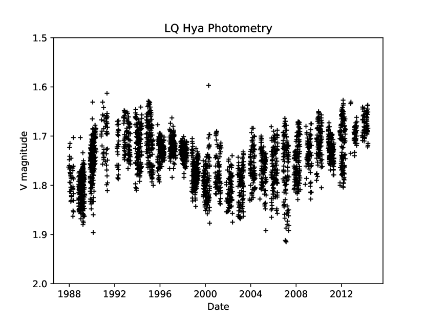
Photometric studies spanning decades can be used to examine the periodicities in the light curve of LQ Hya utilising time series analysis techniques. Jetsu (1993) used a decade of photometry and found an overall cycle period of 6.2 years for the mean brightness. Changes in magnitude also correlated with changes in the observed effective temperature based on the mean colour index. Strassmeier et al. (1997) found a similar cycle fit of about 7 years. With a longer timespan of photometric observations, multiple cycles of 11.4, 6.8, and 2.8 years were observed by Oláh et al. (2000) and cycles of 15 and 7.7 years were reported by Berdyugina et al. (2002). However, the longer the baseline of observations used, the less certain these cycles become as the activity appears to be somewhat chaotic. Only weak indications of a 13 year cycle were detected by Lehtinen et al. (2012) and a weak indication for a 6.9 year cycle was found by Olspert et al. (2015). Lehtinen et al. (2016) suggested a long and seemingly non-stationary cycle with a period somewhere between 14.5 and 18 years as well as some indication for 2 to 3 year oscillatons that could not be demonstrated to be periodic. Oláh et al. (2009) revisited the photometric observations of their previous paper but with a longer dataset and found a 7 year cycle that steadily increased to 12.4 years when a longer timespan of photometry was used. From Figure 1, we can see that cycle periods are difficult to estimate from the limited dataset because the longer cycle estimates are still a significant fraction of the total timespan of data.
Another phenomenon of interest that can be obtained from light curves is the existence of active longitudes, or the tendency of starspots to occur at the same longitude for several years. These active longitudes may sometimes suddenly switch by about , commonly referred to as a flip-flop (Jetsu et al., 1993). Berdyugina et al. (2002) found two active longitudes approximately apart for the duration of their photometric data with a phase drift of about yr-1 in the rotation frame. Lehtinen et al. (2012) detected only one stable active longitude between 2003 and 2009 from their dataset while any other active longitudes were only stable for half a year. This is supported by the carrier fit analysis of Olspert et al. (2015) which finds the rotation periods of spots with linear trends between the epochs 1990–1994, and again for 2003–2009. Lehtinen et al. (2012) found possible flip-flops in late 1988, 1994, 1999, 2000, and 2010. Olspert et al. (2015) found agreement with the 1988, 1999, and 2010 flip-flops and an additional possible flip-flop in late 1997.
Photometry mainly contains longitudinal and stellar magnitude information and can only barely distinguish between high and low latitudes for good datasets (e.g., Berdyugina et al., 2002). In order to study the spot latitudes, inversion methods must be applied to stellar spectra. The Doppler imaging technique (hereafter DI) provides both latitudinal and longitudinal information for cool spots. Using this technique for LQ Hya, Strassmeier et al. (1993) found spotted regions mainly near the pole and equator with larger spot structures extending to mid-latitudes during 1991. Rice & Strassmeier (1998) found similar results from their maps, although the near-polar spots were weaker during 1993 and 1995. Kovári et al. (2004) recovered spots at low- to mid-latitudes for observations during 1996 and 2000 and found the spot evolution to be rapid. They speculated this to be the result of changes in the emergence rate of magnetic flux and not spot migration. Cole et al. (2014) found some evidence for a bimodal structure with spots either at high or low latitudes for seven observing seasons spanning from 1998–2002. Flores Soriano & Strassmeier (2017) reconstructed temperature maps from late 2011 to mid-2012 and found two large near-polar spots and one low-latitude spot that migrated equatorward over the course of the observations.
The Zeeman Doppler imaging technique (hereafter ZDI) yields similar results of bimodal structure with spots either at very low or very high latitudes. Spot occupancy maps from 1991–2002 from Donati (1999) and Donati et al. (2003b) reveal near-polar spots for some observing seasons and spots between the equator and latitudes corresponding to the radial and azimuthal magnetic field components with components measuring as high as 900 G and a mean quadratic magnetic field flux between 30–100 G. Furthermore, they found that the assumed relationship of Berdyugina et al. (2002) between dark, low latitude spots and photometric minima to not be upheld by the ZDI results, but rather, dependent on multiple phenomena such as the nonaxissymetric polar features. Donati et al. (2003b) also observed that the spot evolution is not the result of equatorward drift of spots from high to low latitudes, but rather seems to the result of some other mechanism that causes high and low latitude spots to form at varying strengths over time.
The surface differential rotation of LQ Hya appears to be small. Estimates from photometry range from – where and is the rotation rate at the equator and is the rotation rate at the poles (Jetsu, 1993; You, 2007; Olspert et al., 2015). Berdyugina et al. (2002) tracked active longitudes and estimated a differential rotation rate of based on the period differences. Estimates from DI give a similarly small differential rotation rate of (Kovári et al., 2004), and Donati et al. (2003a) find from ZDI maps that the measured differential rotation switches between almost solid body rotation () and weak differential rotation () . Thus, the differential rotation measurements are not conclusive, but all reported results point to a small -value. Hence, in this study we do not include differential rotation into the inversion procedure.
Evidently, the star seems highly variable in its spot activity, with periods of long-lived spot structure and periods of chaotic and rapid spot evolution. As Lehtinen et al. (2016) note, from the photometry alone it becomes apparent that while LQ Hya was cyclical for earlier epochs, it seems now to be steadily increasing in surface brightness with no overt signs of stopping (see Figure 1). The only exception to this upward trend is a slight dip in the curve downward between 2009–2011. Such a trend would indicate an increase in the magnetic activity level of the star. This paper aims to examine the spot topology of LQ Hya from 2006–2017 using the DI technique during this period of decreasing activity level.
2 Data
| Instrument | Date | HJD | S/N | Instrument | Date | HJD | S/N | ||
| (dd/m/yyyy) | -2 400 000 | (dd/m/yyyy) | -2 400 000 | ||||||
| SOFIN | 02/12/2006 | 54071.7383 | 0.548 | 168 | SOFIN | 13/12/2011 | 55908.7461 | 0.863 | 418 |
| SOFIN | 03/12/2006 | 54072.7578 | 0.185 | 289 | SOFIN | 14/12/2011 | 55909.6992 | 0.458 | 434 |
| SOFIN | 04/12/2006 | 54073.7617 | 0.812 | 185 | SOFIN | 15/12/2011 | 55910.7305 | 0.102 | 224 |
| SOFIN | 05/12/2006 | 54074.7422 | 0.424 | 221 | SOFIN | 23/11/2012 | 56254.7461 | 0.960 | 360 |
| SOFIN | 06/12/2006 | 54075.7461 | 0.051 | 214 | SOFIN | 28/11/2012 | 56259.7539 | 0.087 | 298 |
| SOFIN | 23/11/2007 | 54427.7695 | 0.909 | 215 | SOFIN | 04/12/2012 | 56265.7500 | 0.832 | 333 |
| SOFIN | 27/11/2007 | 54431.7695 | 0.408 | 179 | SOFIN | 05/12/2012 | 56266.7539 | 0.459 | 369 |
| SOFIN | 28/11/2007 | 54432.7734 | 0.035 | 272 | SOFIN | 15/11/2013 | 56611.7461 | 0.926 | 229 |
| SOFIN | 01/12/2007 | 54435.7695 | 0.906 | 217 | SOFIN | 20/11/2013 | 56616.7695 | 0.064 | 196 |
| SOFIN | 02/12/2007 | 54436.7695 | 0.530 | 268 | SOFIN | 21/11/2013 | 56617.7656 | 0.686 | 336 |
| SOFIN | 03/12/2007 | 54437.7773 | 0.160 | 217 | SOFIN | 22/11/2013 | 56618.7656 | 0.310 | 362 |
| SOFIN | 09/12/2008 | 54809.7031 | 0.449 | 422 | FIES | 03/12/2014 | 56994.7070 | 0.107 | 280 |
| SOFIN | 10/12/2008 | 54810.7383 | 0.095 | 205 | FIES | 05/12/2014 | 56996.6563 | 0.325 | 290 |
| SOFIN | 11/12/2008 | 54811.6992 | 0.695 | 297 | FIES | 07/12/2014 | 56998.7070 | 0.605 | 215 |
| SOFIN | 12/12/2008 | 54812.7148 | 0.330 | 251 | FIES | 08/12/2014 | 56999.7148 | 0.235 | 210 |
| SOFIN | 15/12/2008 | 54815.7578 | 0.230 | 67 | FIES | 26/11/2015 | 57352.7656 | 0.735 | 60 |
| SOFIN | 27/12/2009 | 55192.6953 | 0.649 | 316 | FIES | 27/11/2015 | 57353.7227 | 0.333 | 180 |
| SOFIN | 30/12/2009 | 55195.6914 | 0.520 | 317 | FIES | 28/11/2015 | 57354.7227 | 0.957 | 190 |
| SOFIN | 31/12/2009 | 55196.6758 | 0.135 | 223 | FIES | 30/11/2015 | 57356.7227 | 0.206 | 180 |
| SOFIN | 01/01/2010 | 55197.6836 | 0.764 | 373 | FIES | 03/12/2015 | 57359.6914 | 0.061 | 240 |
| SOFIN | 05/01/2010 | 55201.6328 | 0.231 | 304 | FIES | 19/12/2017 | 58106.6914 | 0.604 | 170 |
| SOFIN | 14/12/2010 | 55544.6797 | 0.483 | 330 | FIES | 20/12/2017 | 58107.5547 | 0.143 | 210 |
| SOFIN | 23/12/2010 | 55553.7461 | 0.146 | 376 | FIES | 20/12/2017 | 58107.7734 | 0.280 | 240 |
| SOFIN | 24/12/2010 | 55554.7305 | 0.760 | 405 | FIES | 21/12/2017 | 58108.6953 | 0.856 | 220 |
| SOFIN | 25/12/2010 | 55555.7461 | 0.395 | 351 | FIES | 22/12/2017 | 58109.5859 | 0.412 | 120 |
| SOFIN | 26/12/2010 | 55556.7656 | 0.031 | 283 | FIES | 22/12/2017 | 58109.7148 | 0.493 | 180 |
| SOFIN | 09/12/2011 | 55904.7305 | 0.355 | 363 | FIES | 23/12/2017 | 58110.5977 | 0.044 | 240 |
| SOFIN | 11/12/2011 | 55906.7188 | 0.597 | 251 | FIES | 23/12/2017 | 58110.7383 | 0.132 | 290 |
| SOFIN | 12/12/2011 | 55907.7422 | 0.236 | 293 |
We have collected 11 sets of winter-season spectra, covering the time interval 2006–17, with the 2.56 m Nordic Optical Telescope at La Palma, Spain. The details of the observations are given in Table 1 and the season summaries in Table 2. For the years 2006–2013 we used the SOFIN instrument, which is a high-resolution échelle spectrograph mounted in the Cassegrain focus, while for the years 2014–2017 we used FIES, which is a fiber-fed échelle spectrograph. The former has also a spectropolarimetric mode available, but in this paper we only analyse the unpolarised spectroscopy obtained with the two instruments, the aim being to monitor the behaviour of starspots in terms of temperature anomalies on the stellar surface. The SOFIN observations were reduced with the new SDS tool, which is described in some detail in Willamo et al. (2019). The FIES observations were reduced with the standard FIEStool pipeline (Telting et al., 2014). The spectral resolutions of SOFIN and FIES data sets are 70 000 and 67 000, respectively. The observations have mostly poor to moderate phase coverage of 39–68%, while the signal-to-noise ratio (hereafter S/N) is reasonably good with mean values exceeding 200 for all but one season.
For phasing the observations, we used the rotation period and the ephemeris from Jetsu (1993),
| (1) |
where corresponds to the zero phase. Other stellar parameters adopted, listed in Table 3, closely follow those of Cole et al. (2015), except for the surface gravity and microturbulence values. For the former, we used a more standardly reported value of (Tsantaki et al., 2014), while for latter, we adopted a somewhat higher value of = 1.5 km s-1, found by fitting the mean spectral lines from all seasons of our data to a model calculated for an unspotted surface.
The spectral regions 6438.4–6439.8 Å, 6461.8–6463.5 Å, and 6471.0–6472.4 Å were used for SOFIN observations, while for FIES, three additional spectral regions of 6410.9–6412.4 Å, 6419.3–6422.0 Å, and 6430.2–6431.5 Å were used. The FIES spectral regions overlap both with those used by Cole et al. (2015) and the SOFIN observations in this paper.
| Time | Instrument | S/N | [%] | [%] | |
| Dec 2006 | SOFIN | 5 | 215 | 50 | 0.542 |
| Dec 2007 | SOFIN | 6 | 228 | 53 | 0.491 |
| Dec 2008 | SOFIN | 5 | 248 | 50 | 0.936 |
| Dec 2009 | SOFIN | 5 | 306 | 50 | 0.388 |
| Dec 2010 | SOFIN | 5 | 344 | 49 | 0.412 |
| Dec 2011 | SOFIN | 6 | 268 | 60 | 0.448 |
| Dec 2012 | SOFIN | 4 | 340 | 40 | 0.380 |
| Nov 2013 | SOFIN | 4 | 281 | 40 | 0.496 |
| Dec 2014 | FIES | 4 | 249 | 39 | 0.425 |
| Dec 2015 | FIES | 5 | 170 | 50 | 0.637 |
| Dec 2017 | FIES | 8 | 209 | 68 | 0.549 |
3 Doppler imaging
| Parameter | Value |
|---|---|
| Effective temperature | = 5000 K |
| (unspotted) | |
| Gravity | log = 4.5 |
| Inclination | = 65∘ |
| Rotational velocity | = 26.5 km s-1 |
| Rotation period | = 1601136 |
| Metallicity | log[M/H] = 0 |
| Microturbulence | = 1.5 km s-1 |
| Macroturbulence | = 1.5 km s-1 |
To invert the observed spectroscopic line profiles into a surface temperature distribution on the stellar surface, we used the DI code INVERS7DR (see e.g. Willamo et al., 2019), that uses Tikhonov regularisation for the ill-posed inversion problem (Piskunov et al., 1990). The regularisation technique minimises temperature gradients in the solution and hence tends to damp small-scale features.
To construct a model spectrum for the star, we retrieved the spectral parameters from the Vienna Atomic Line Database (Kupka et al., 1999; Ryabchikova et al., 2015), using effective temperatures of 5000 K and 4000 K for the unspotted and spotted stellar surface, respectively. We used a total of 114 lines for the SOFIN spectral regions, and 221 lines for the FIES spectral regions for the computation of the synthetic spectra. Line profiles were calculated using plane-parallel stellar atmosphere models taken from the MARCS database (Gustafsson et al., 2008). The lines used for inversions are Fe I and Ca I lines. We assume solar metallicity and adjust individual spectral lines to fit the mean observations. The stellar lines used and their original and adopted parameters are listed in Table 4. The Ca I lines are susceptible to non-local thermal equilibrium (NLTE) effects in the temperature range of LQ Hya, but a simple test excluding these lines from the inversion procedure did not alter the results significantly. The NLTE effects were likely mitigated by our use of a higher value for . The models covered the temperature range 3500–6000 K.
| Line [Å] | ||
|---|---|---|
| Fe I | ||
| Fe I | ||
| Fe I | ||
| Fe I | ||
| Ca I | ||
| Fe I | ||
| Ca I |
The surface grid resolution used for the inversion was in latitude and longitude, respectively. The inversion was run with the regularisation parameter for 100 iterations, at which point a sufficient convergence was reached. The final deviation between the inversion solution and the observations is indicated in the sixth column in Table 2. We constrained the inversion process by imposing lower and upper temperature limits of 3500 K and 5500 K, respectively. This was necessary because our observations generally have only a modest phase coverage and the inversions tend to produce features with very high temperatures as a result. Such features are not likely to be physically real for a cool star such as LQ Hya and so we adopted the upper temperature limit. The temperature constraint was done by adding a penalty function to the minimisation procedure as described in Hackman et al. (2001). In all cases this procedure was not observed to change the overall topology of the solution.
4 Results
4.1 Temperature maps from SOFIN observations, 2006–2013
We use the DI technique and solve for the surface temperature for each of the observing season. Our S/N is good for all but two of the individual observations, but all observations within a season are weighted based on their S/N so that noisier observations have less of an impact on the final map. Despite the good S/N, our results still need to be treated with some reservation because we have poor to moderate phase coverage for most of our seasons. From Table 2 we can see that the best seasons are Dec.2011 and Dec.2017 with a of 60% and 68% respectively, where was calculated by assuming a phase range of for each observation. All other seasons have a of 53% or less and thus interpretation of the maps should be treated carefully. This will be addressed further in Section 5.
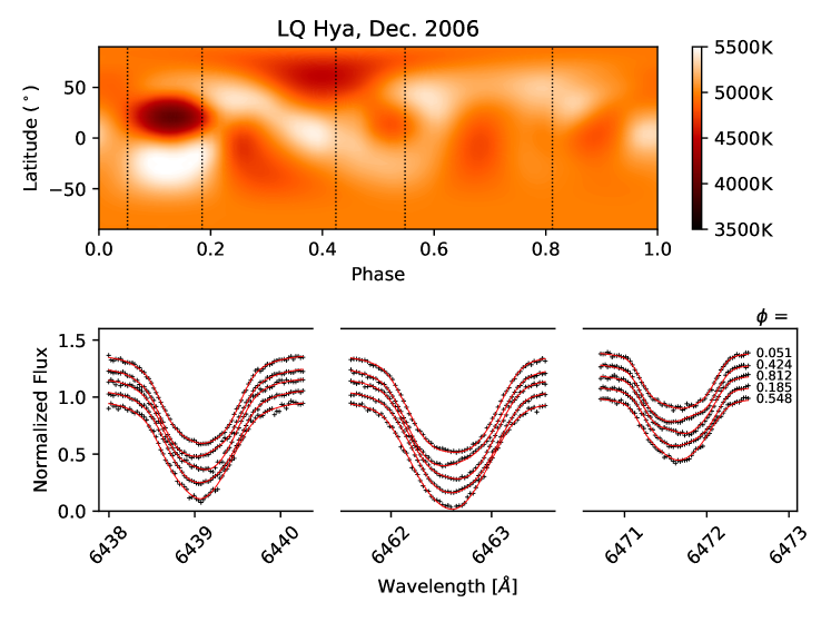
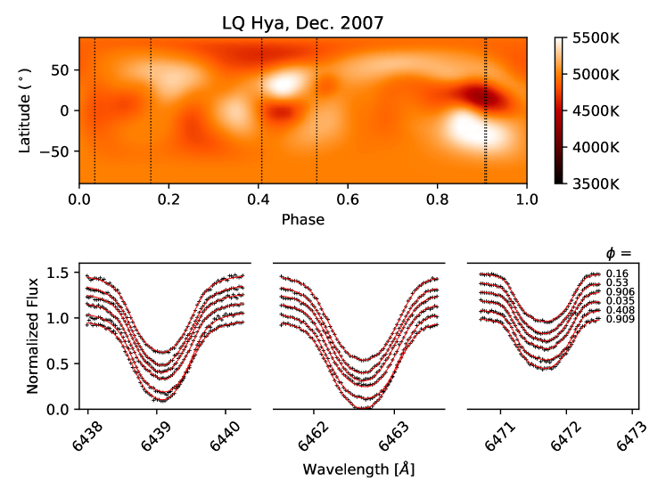
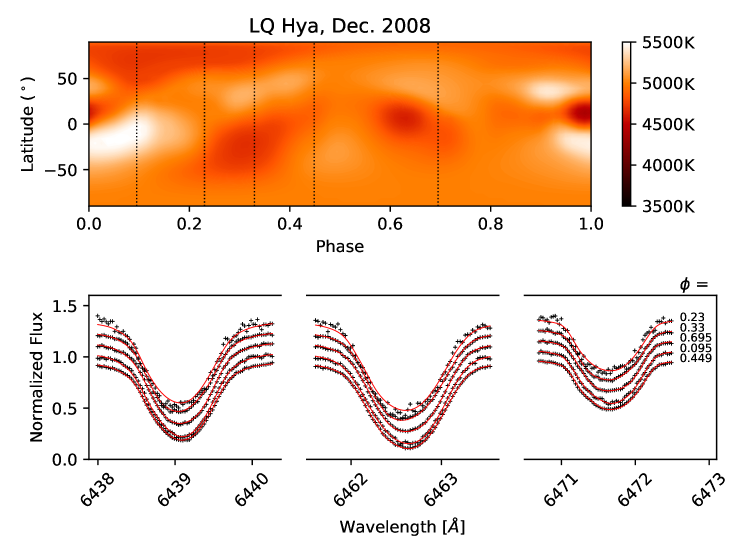
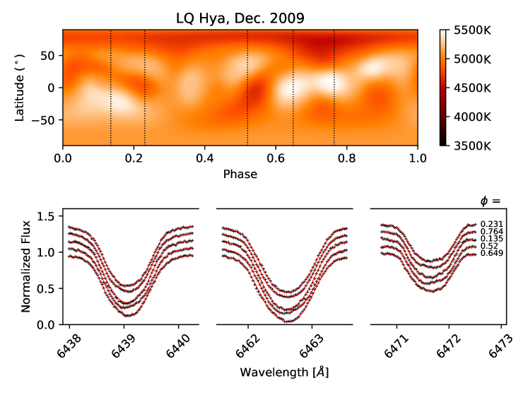
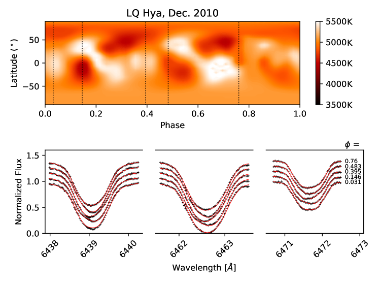
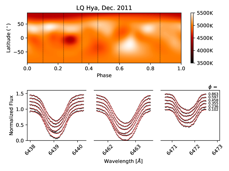
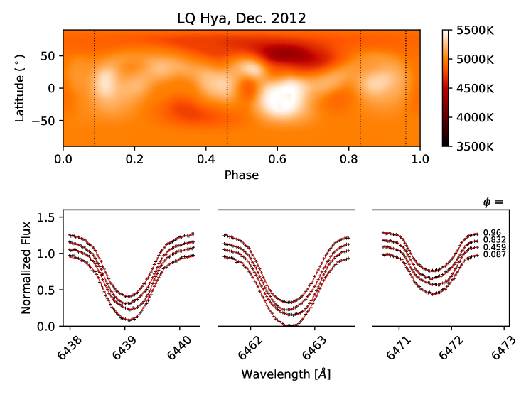
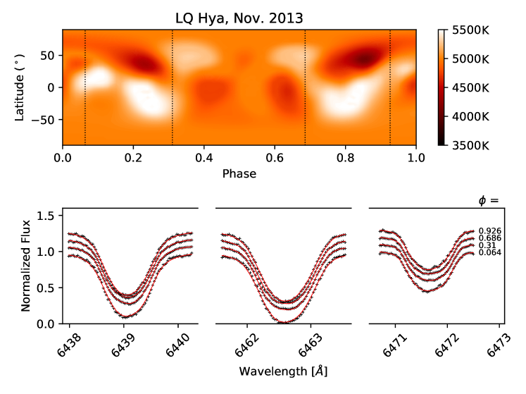
Temperature maps for the SOFIN observations are presented in Figure 2.
-
•
The Dec.2006 observing season has a 50% phase coverage. The cool spot near phase 0.12 is latitudinally paired with a hot spot, which are likely artefacts. There is evidence of a cool spot at high latitudes at phase around 0.4, but no evidence of a secondary high-latitude spot structure at phase 0.8, which agrees with the photometric results of Olspert et al. (2015): during 2006–2010, the spot evolution was primarily dominated by one spot that showed rather chaotic phase behaviour.
-
•
The Dec.2007 observations have a phase coverage of 53% and exhibit some artefacts in the area of the large phase gap of . We again find evidence for a large high-latitude spot around phase 0.4, hence the primary spot structure seems to still appear at the same longitude as during the previous year, which is not in good agreement with photometry of Olspert et al. (2015), which indicates primary spot structure at around phase 0.9 and a secondary spot at phase 0.4. There are also two low-latitude cool spots paired with hot spots at the same phase, but these might be artefacts.
-
•
The Dec.2008 observations show cool spots both near the equator and near the poles but the phase coverage is 50% and the observation at is noisy. This may cause the inversion program to produce artificial spots near that particular phase. The primary high-latitude spot structure now appears close to phase 0, which agrees better with the photometry of Olspert et al. (2015). Of the equatorial spots the ones close to phase 0.4 and 0.6 seem realistic, although there are weak hot shadows paired with them at higher latitudes.
-
•
In Dec.2009, with a phase coverage of 50%, we get a very strong high-latitude spot structure with a temperature minimum around the phase 0.75. The structure is elongated in phase, almost forming an asymmetric cool polar cap. The location of the temperature minimum matches well with photometry of Olspert et al. (2015). Again, lower latitude features are abundant, but paired hot shadows at the same phase accompany most of them. In between phases 0.6 and 1.0 we see a 4-leaf clover structure of two of these features, cool-hot and hot-cool pair adjacent to each other. Such a feature can be caused by a spot close to the visible southern limb, but can also be an artefact.
-
•
The observations for Dec.2010 have a phase coverage of 49% and the map seems to be dominated by artefacts with no evidence of high-latitude activity. We see a checkerboard pattern around the equator at all phases, most likely resulting from the combination of poor phase coverage with a long observation period during which the star may have changed. Just by inspecting the line profiles, one sees strong spot variability, but it is impossible to judge which of the features in the map itself are real and which are artefacts. Photometry indicates again one primary spot structure around phase 0.6, where no spectroscopy is available. After this season, the star appears to enter a very chaotic state, characterised by frequent phase jumps, which were classified as flip-flops by Olspert et al. (2015).
-
•
Dec.2011 is our best SOFIN season with a 60% phase coverage. The inverted map shows both cool spots at equatorial and high latitudes with middle latitudes devoid of spots. The strongest temperature minimum occurs at around phase 0.1, but the high-latitude spot structure is again very elongated, possibly forming an asymmetric cool polar cap on the star.
-
•
The Dec.2012 season has a phase coverage of 40% and the single cool spot at mid-latitudes appears in the largest gap between observed phases and may thus be an artefact. The typical high-latitude structures seem not to be present any longer.
-
•
The Nov.2013 map shows again a checkerboard pattern and the phase coverage is only 40%. Cool spots in this map appear at mid-latitudes and are paired with warmer spots that are probably artefacts. Again, high-latitude structures are absent.
4.2 Temperature maps from FIES observations, 2014, 2015, and 2017
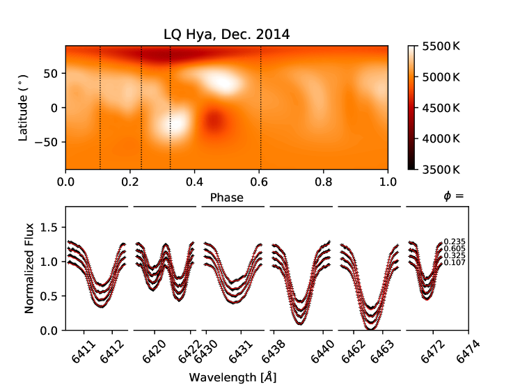
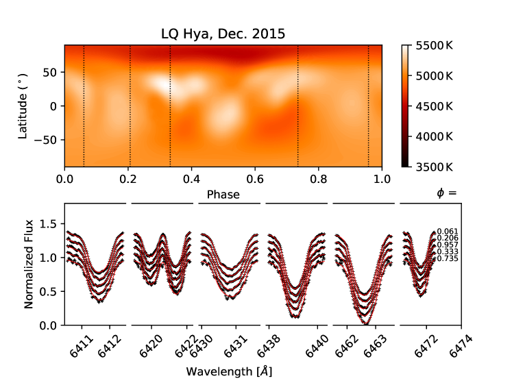
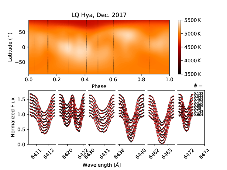
Figure 3 shows the FIES maps where three additional Fe I lines were selected to overlap with those used by Cole et al. (2015).
-
•
Phase coverage for Dec.2014 is again poor, with of only 39%. After several years of absence of high-latitude activity, we now recover an extended high-latitude spot structure with a temperature minimum around the phase 0.3. Even though the phase coverage is poor, this structure coincides with the observed phases and is most likely real. Whether it would extend even more in phase is, however, unclear due to the large phase gap from 0.6–1.1. An equatorial spot is also retrieved, but as it is paired with a hot spot, it could be an artefact.
-
•
Dec.2015 has a slightly better phase coverage of 50%, but the observations at are noisy. There is again evidence of a cool spot near the pole. The temperature minimum of the retrieved structure occurs in a relatively large phase gap, hence the real longitudinal extent and the exact location of the temperature minimum remain uncertain.
-
•
Dec.2017 is considered our best map, with eight observations and a phase coverage of 68%. This map shows a cool spot near the polar region, the temperature minimum occurring at around phase 0.4, and no spots near the equatorial region.
4.3 Overall behaviour and comparison to earlier works
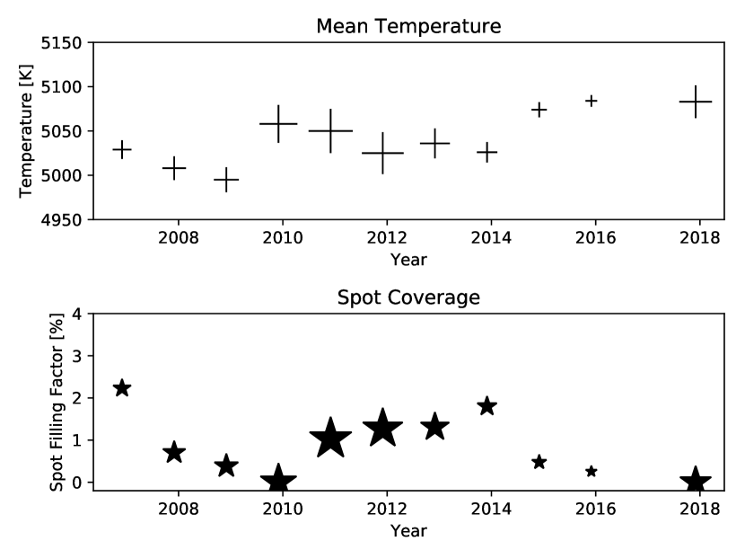
Figure 4 shows the changes in the mean temperature and spot filling factor over time. The symbol size is proportional to so that larger symbols emphasize the degree of confidence arising from higher S/N and better phase coverage. The spot filling factor was calculated as the percentage of the surface area covered by spots, defined as regions colder than 4500 K. As previously shown by Willamo et al. (2019) and Hackman et al. (2019), the relative changes in spot coverage are not very sensitive to the defined spot temperature. From the top panel of Figure 4, it can be seen that there is a trend of increasing mean temperature, which corresponds fairly well with the observed brightening of the star between 2006 and 2014 seen in Figure 1. Because spot coverage is overestimated with poor phase coverage, only the large symbols are reliable and thus we can really only conclude that the spot coverage around Dec.2011 was greater than the virtually unspotted season of Dec.2017. Nevertheless, the slight hint of an overall decreasing trend of spot coverage is consistent with the increase in the mean temperature, and hence supports our hypothesis of the star entering a low activity state. Moreover, if we compare our results to the spot coverage results for Cole et al. (2015), we find that LQ Hya is less spotted overall during these more recent observations.
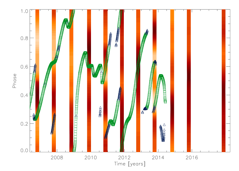
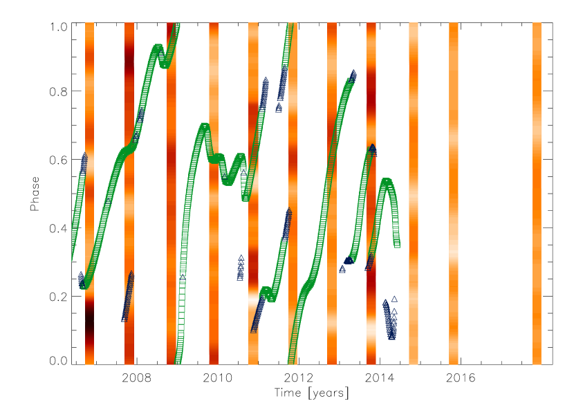
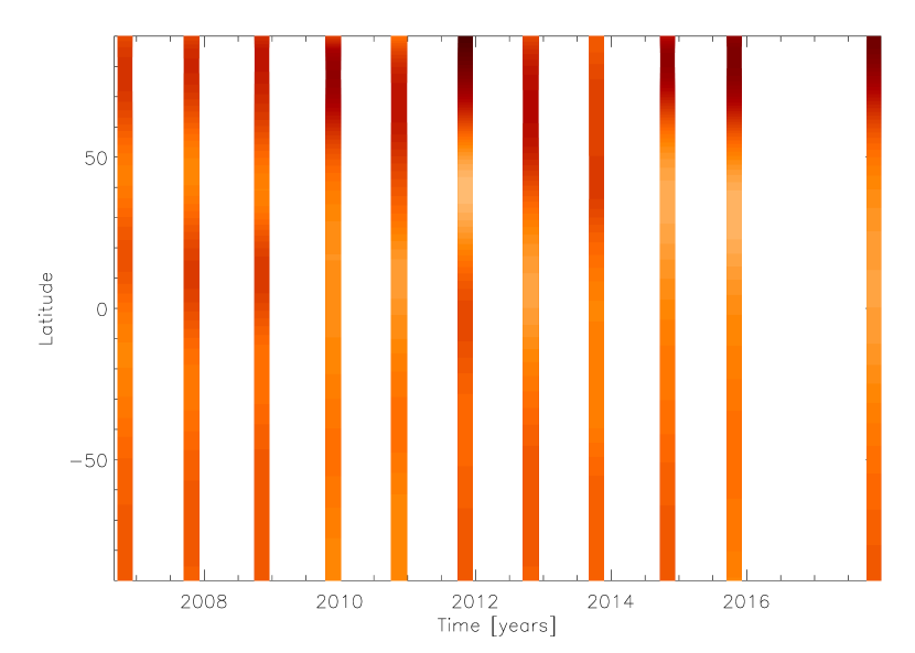
Spot latitudes, particularly those at lower latitudes, should be treated with some skepticism because of the poor phase coverage for most of the observing seasons and low latitude spots paired with hot spots can be treated as possible weakly cool spots or artefacts. However, we consider the spot phases to be robust. To try to minimise the effect of the low latitude spot structures, most likely artefacts, we split our latitudinal averages of the temperature at each phase into two categories: high-latitude spots, those above , and low-latitude spots, those in between the equator and . No spots below latitude can be observed due to the inclination angle of the star and so we use the northern hemisphere only for the averages. The reports of various authors that the mid-latitude region is void of spots also motivates this approach (Strassmeier et al., 1993; Rice & Strassmeier, 1998; Donati, 1999; Donati et al., 2003a; Cole et al., 2014). We then plot these in Figure 5 against the photometric minima of Olspert et al. (2015). From the top and middle panels of Figure 5, it can be seen that the photometric minima are in better agreement with the phases of high latitude spots (top) than with those at low latitudes (middle).
In the bottom panel of Figure 5, we take the average over each latitude to see what latitudes spots tend to form at. During all observing seasons except Dec.2010, 2012, and 2013, we find that there are cool spots at high latitudes (Figures 2, 3). These observations without high latitude spots suffer from poor phase coverage, so we cannot exclude the possibility that such spots also exist for these seasons, just that they did not fall near the phases of our observations. However, the typical high-latitude spot structures have usually large phase extents, and during other observing seasons with equally poor phase coverage we do recover them. Hence, it is possible that during the chaotic state beginning in 2010, the high-latitude spot structure was suppressed. In 2014 and from there onwards, the high-latitude spot structure recovers. Of the two maps with the best phase coverage, Dec.2011 and Dec.2017, we find that Dec.2011 has both spots at high and low latitudes, while Dec.2017 has only the spot at a high latitude. We see some bimodality (spots appearing at only high and low latitudes) in Figure 5, bottom, for the SOFIN observations but this is not as pronounced for the FIES observations. However, this must be taken with a grain of salt because, as previously discussed, latitudinal information particularly for low latitude spots is lost with poor phase coverage.
Rice & Strassmeier (2000) found that phase gaps as large as still reproduced spot phases from an artificial map containing large spots, although the spot temperatures and shape were changed. Our phase gaps are somewhat larger for some seasons, but we find the areas between our larger phase gaps to be relatively smooth in temperature gradients with the exception of the Dec.2008 and Dec.2012 maps, which have cool spots in the large phase gaps. Lindborg et al. (2014) used a temperature map of DI Piscium from an observing season with good phase coverage and removed all but five observations and found that a previously weak cool spot increased in contrast and a corresponding hot spot formed at the same phase. Thus we would expect then that our low-latitude, cool spots, if physical, when paired with hot spots are actually weaker cool spots at those phases and the hot spots are likely not physical. In Cole et al. (2015) it was seen that poor phase coverage increases the temperature contrast by 300 K which results in an overestimate of spot coverage. The mean temperature however changed by only 10 K. Thus we expect our temperature differences to be dependent on the phase coverage, increasing with poorer coverage. As the spot filling factor is calculated from this quantity, this result would be correspondingly shifted to a higher value and hence our results are more of an upper limit. However, the mean temperature was found to shift by very little in all cases, and so our results of mean temperature are considered more robust than the spot filling factor and the spot temperature.
The bimodality of the spot distribution with very few spots at mid-latitudes was also observed in DI maps from earlier epochs, such as those by Rice & Strassmeier (1998) and Cole et al. (2015). We do not find a band of spots around the latitude as was the case for Kovári et al. (2004), although this may be explained by our lower value for . Flores Soriano & Strassmeier (2017) also performed a Doppler imaging analysis of LQ Hya during December 2011 with some overlap of similar spectral lines for Fe I and Ca I as in our study. The Doppler maps closest in time to our Dec.2011 map have two near-polar spots and one spot close to the equator. Our maps seem to agree with this spot configuration, with our Dec.2011 map showing a large spot near the polar region and another spot closer to the equator. Their phase for the low-latitude spot is different from our phase by when accounting for the different ephermeris, but the midpoint of the two high-latitude spots does match the phase of our elongated high-latitude feature. This map also had decent phase coverage, so the equatorial spot is likely physical. A persistent spot near the pole is also observed in the ZDI maps of Donati (1999) and Donati et al. (2003b), and this was found to be similarly nonaxisymmetric.
Contemporaneous observations in photometry to measure periodicities and study the phenomena of active longitudes and flip-flops are of interest when examining the maps. Olspert et al. (2015) found evidence of a flip-flop during late 2010, and phase disruptions during 2012 and 2013. They also found evidence of a phase drift during 2008. Lehtinen et al. (2012) found flip-flop behaviour during their late-2010/early-2011 observations. The recovered spots in our Dec.2010 map are close to the phases of the light-curve minima and so while the higher temperature contrast is likely an artifact, the spots themselves would be physical, revealing a rather chaotic surface during this epoch corresponding with the chaos from flip-flops and phase jumps found in the photometry. Visual inspection of the spectral lines for Dec.2010 in Figure 2 reveals significantly changed line profiles in between rather small changes in phase, supporting the chaotic surface temperature map of this season.
The photometric minima, indicating active regions, have been well-matched to indicators of chromospheric activity for LQ Hya. Cao & Gu (2014) matched their phases of observations from 2006–2012 of plage regions to the photometry of Lehtinen et al. (2012) and found an increase in chromospheric activity corresponded to a decrease in photometric magnitude. Cao & Gu (2014) also found that the chromospheric activity level in general steadily decreased throughout their observations from 2006–2012, which matches the increase in magnitude in photometry seen during this time as well as the increase in the mean temperature in our maps. Cao & Gu (2014) found a plage region in Febuary 2012. If we convert their observations to our ephemeris in Equation 1, we find their plage region occurs at which coincides with our low-latitude spot near that phase.
The zonal models of Livshits et al. (2003) limit spots to two latitudinal belts symmetric about the equator and examines the shift in the upper and lower latitudinal boundaries, a rough approximation of the butterfly diagrams of the Sun. For the epochs 1983–2001, they find that a rise in activity level corresponds to an equatorward drift of the lower latitudinal boundary of the spot zones, where the relative spotted area is used as the indicator of activity. The upper boundary of the zone remained somewhat constant and was relatively low (). However, we find mainly high-latitude or low-latitude spots and not many in the – range, and from Figure 5, bottom, we see that our low-latitude spots get weaker from Dec.2014 to Dec.2017 while the high-latitude spot remains. During the chaotic period between Dec.2010–2013, spots and both higher and lower latitudes appear and disappear from season to season, although some of this may be due to poor phase coverage.
5 Discussion on the data quality and effects on the maps
Poor phase coverage is the primary source of artefacts in most of our maps. Spots located at or near the observed phases, indicated by vertical dashed lines in Figures 2 and 3, are likely physical as the S/N in these observations were high. Furthermore, the evidence of spots is supported by visual inspection of the spectral lines in each figure. For phases not adequately covered by observations, the inversion program lacks information, and the result in cases where spots are near the observed phases is the checkboard pattern seen in, for example, the Dec.2010 map (Figure 2). The inversion program does not introduce spurious spots into areas between the phase gaps but it may increase the temperature contrast of spots further away from the observed phases, such as those seen in our Dec.2008 and Dec.2012 maps (Figure 2).
When phase coverage is poor, the recovered latitudes of spots are also less precise, particularly for spots at lower latitudes. Additionally, the ability of the inversion program to distinguish between low latitude spots above or below the equator worsens with poor phase coverage. Furthermore, LQ Hya is an active star, and while spot structures generally persist for a month or more, sudden changes are possible, as is indicative from photometry especially for 2010-2013. Therefore, due to such rapid changes, spots at higher latitudes may be interpreted as spots at lower latitudes. We consider the effects of rapid variability by examining our Dec.2007 and Dec.2017 maps, both of which had two observations close in phase but distant in time by eight and three days, respectively. Running the inversion excluding first the later observation and then the earlier observation showed no significant difference in the resulting temperature maps around the observed phases beyond a slight change in spot shape. We also keep in mind that the star seems to be decreasing in activity level, and all our observing seasons are 12 days or less, making this source of artefacts less likely. Because of the limitations of the inversion method and poor phase coverage, the spot phases and spots at high latitudes should be more reliable than low latitude spots.
6 Conclusions
We have calculated surface temperature maps for LQ Hya for 11 observing seasons ranging from December 2006 to December 2017 epoch using the DI technique. We summarize our findings as follows:
-
•
Seasons with poorer phase coverage are less reliable, particularly for quantities like the spot latitude and especially for the spots seen at near-equatorial regions. However, spot phases are still robust, and the high-latitude spots are likely physical, while the accuracy of low-latitude spots depends on the phase coverage.
-
•
We find an increase in mean temperature throughout the observing seasons with only a slight dip between 2009 and 2011. This matches the increase in the observed magnitude of the star during this time, indicating a decrease in stellar activity.
-
•
The primary and secondary minima from concurrent photometry better match the phases of high-latitude spots than the phases of low-latitude spots.
-
•
There appears to be a bimodal spot distribution over latitude, which is in agreement with previous DI and ZDI maps of LQ Hya. However, the lower latitude spots become weaker as the activity level of the star decreases while the higher latitude spots persist during the observing seasons with FIES. Both higher and lower latitude spots appear and disappear from season to season with SOFIN.
-
•
Photometry indicates an especially chaotic epoch of spot evolution during 2010–2013, with rapid spot migration in the rotational frame, and abrupt phase changes, that were characterised as flip-flop events by Olspert et al. (2015). Spectroscopy during this time indicates strong line profile variability, indicative of large spottedness, but the maps show checkerboard patterns. Also, the high-latitude spot structures disappear for 2010, 2012, and 2013. Characterising the spot structures from Doppler images is very challenging during this epoch.
Based on our results, LQ Hya seems to be approaching an activity minimum. During a higher activity state, investigated through Doppler imaging by Cole et al. (2015), temperature maps showed mean temperatures K lower than in this study. Those temperature maps, while having a lower S/N on average, show more disruption and bumps in the spectral lines than the ones presented here. Even though the activity is decreasing, the spot structures are still largely chaotic where the lower latitude spots do not appear to form at any preferred longitude. This matches what is found in numerical simulations, such as those by Viviani et al. (2018), where rapid rotation led to a dominance of the non-axisymmetric portion of the magnetic field. Their solutions with roughly twenty times solar rotation rate showed strong high-latitude magnetic fields organised in two active longitudes of opposite polarity on the same hemisphere, while a weaker near-equator activity belt was accompanying these structures.
Acknowledgements.
EC acknowledges funding from the the Deutsche Forschungs-Gemeinschaft (DFG project 4535/1-1). MJK and JL acknowledge the Academy of Finland ”ReSoLVE” Centre of Excellence (project number 307411) and the Max Planck Research Group ”SOLSTAR” funding. OK acknowledges support by the Knut and Alice Wallenberg Foundation (project grant “The New Milky Way”), the Swedish Research Council (project 621-2014-5720), and the Swedish National Space Board (projects 185/14, 137/17).References
- Berdyugina (2005) Berdyugina, S. V. 2005, Living Reviews in Solar Physics, 2, 8
- Berdyugina et al. (2002) Berdyugina, S. V., Pelt, J., & Tuominen, I. 2002, A&A, 394, 505
- Bopp & Evans (1973) Bopp, B. W. & Evans, D. S. 1973, MNRAS, 164, 343
- Cao & Gu (2014) Cao, D.-t. & Gu, S.-h. 2014, AJ, 147, 38
- Cole et al. (2014) Cole, E., Käpylä, P. J., Mantere, M. J., & Brandenburg, A. 2014, ApJ, 780, L22
- Cole et al. (2015) Cole, E. M., Hackman, T., Käpylä, M. J., et al. 2015, A&A, 581, A69
- Donati (1999) Donati, J.-F. 1999, MNRAS, 302, 457
- Donati et al. (2003a) Donati, J.-F., Collier Cameron, A., & Petit, P. 2003a, MNRAS, 345, 1187
- Donati et al. (2003b) Donati, J.-F., Collier Cameron, A., Semel, M., et al. 2003b, MNRAS, 345, 1145
- Fekel et al. (1986) Fekel, F. C., Bopp, B. W., Africano, J. L., et al. 1986, AJ, 92, 1150
- Flores Soriano & Strassmeier (2017) Flores Soriano, M. & Strassmeier, K. G. 2017, A&A, 597, A101
- Gustafsson et al. (2008) Gustafsson, B., Edvardsson, B., Eriksson, K., et al. 2008, A&A, 486, 951
- Hackman et al. (2019) Hackman, T., Ilyin, I., Lehtinen, J. J., et al. 2019, A&A, in press [arXiv:1812.02013]
- Hackman et al. (2001) Hackman, T., Jetsu, L., & Tuominen, I. 2001, A&A, 374, 171
- Hinkel et al. (2017) Hinkel, N. R., Mamajek, E. E., Turnbull, M. C., et al. 2017, ApJ, 848, 34
- Jetsu (1993) Jetsu, L. 1993, A&A, 276, 345
- Jetsu et al. (1993) Jetsu, L., Pelt, J., & Tuominen, I. 1993, A&A, 278, 449
- Kovári et al. (2004) Kovári, Z., Strassmeier, K. G., Granzer, T., et al. 2004, A&A, 417, 1047
- Kupka et al. (1999) Kupka, F., Piskunov, N., Ryabchikova, T. A., Stempels, H. C., & Weiss, W. W. 1999, A&AS, 138, 119
- Lehtinen et al. (2012) Lehtinen, J., Jetsu, L., Hackman, T., Kajatkari, P., & Henry, G. W. 2012, A&A, 542, A38
- Lehtinen et al. (2016) Lehtinen, J., Jetsu, L., Hackman, T., Kajatkari, P., & Henry, G. W. 2016, A&A, 588, A38
- Lindborg et al. (2014) Lindborg, M., Hackman, T., Mantere, M. J., et al. 2014, A&A, 562, A139
- Livshits et al. (2003) Livshits, M. A., Alekseev, I. Y., & Katsova, M. M. 2003, Astronomy Reports, 47, 562
- Montes et al. (2001) Montes, D., López-Santiago, J., Fernández-Figueroa, M. J., & Gálvez, M. C. 2001, A&A, 379, 976
- Oláh et al. (2009) Oláh, K., Kolláth, Z., Granzer, T., et al. 2009, A&A, 501, 703
- Oláh et al. (2000) Oláh, K., Kolláth, Z., & Strassmeier, K. G. 2000, A&A, 356, 643
- Olspert et al. (2015) Olspert, N., Käpylä, M. J., Pelt, J., et al. 2015, A&A, 577, A120
- Piskunov et al. (1990) Piskunov, N. E., Tuominen, I., & Vilhu, O. 1990, A&A, 230, 363
- Rice & Strassmeier (1998) Rice, J. B. & Strassmeier, K. G. 1998, A&A, 336, 972
- Rice & Strassmeier (2000) Rice, J. B. & Strassmeier, K. G. 2000, A&AS, 147, 151
- Ryabchikova et al. (2015) Ryabchikova, T., Piskunov, N., Kurucz, R. L., et al. 2015, Phys. Scr, 90, 054005
- Strassmeier et al. (1997) Strassmeier, K. G., Bartus, J., Cutispoto, G., & Rodono, M. 1997, A&AS, 125, 11
- Strassmeier et al. (1993) Strassmeier, K. G., Rice, J. B., Wehlau, W. H., Hill, G. M., & Matthews, J. M. 1993, A&A, 268, 671
- Telting et al. (2014) Telting, J. H., Avila, G., Buchhave, L., et al. 2014, Astronomische Nachrichten, 335, 41
- Tetzlaff et al. (2011) Tetzlaff, N., Neuhäuser, R., & Hohle, M. M. 2011, MNRAS, 410, 190
- Tsantaki et al. (2014) Tsantaki, M., Sousa, S. G., Santos, N. C., et al. 2014, A&A, 570, A80
- Viviani et al. (2018) Viviani, M., Warnecke, J., Käpylä, M. J., et al. 2018, A&A, 616, A160
- Willamo et al. (2019) Willamo, T., Hackman, T., Lehtinen, J. J., et al. 2019, A&A, 622, A170
- Yeo et al. (2014) Yeo, K. L., Krivova, N. A., Solanki, S. K., & Glassmeier, K. H. 2014, A&A, 570, A85
- You (2007) You, J. 2007, A&A, 475, 309