Advection by Compressible Turbulent Flows: Renormalization Group Study of Vector and Tracer Admixture

Abstract

Advection-diffusion problems of magnetic field and tracer field are analyzed using the field theoretic perturbative renormalization group. Both advected fields are considered to be passive, i.e., without any influence on the turbulent environment, and advecting velocity field is generated by compressible version of stochastic Navier-Stokes equation. The model is considered in the vicinity of space dimension $d=4$ and is a continuation of previous work [N.V. Antonov et al., Phys. Rev. E 95, 033120 (2017)]. The perturbation theory near the special dimension $d=4$ is constructed within a double expansion scheme in $y$ (which describes scaling behavior of the random force that enters a stochastic equation for the velocity field) and $\varepsilon=4-d$. We show that up to one-loop approximation both types of advected fields exhibit similar universal scaling behavior. In particular, we demonstrate this statement on the inertial range asymptotic behavior of the correlation functions of advected fields. The critical dimensions of tensor composite operators are calculated in the leading order of $(y,\varepsilon)$ expansion.

Keywords

fully developed turbulence, magnetohydrodynamics, advection-diffusion problem, field-theoretic renormalization group, anomalous scaling

¹ Department of Physics, Saint Petersburg State University,
7/9 Universitetskaya Naberezhnaya, Saint Petersburg 199034, Russia,
² Faculty of Sciences, P.J. Šafárik University, Moyzesova 16, 040 01 Košice, Slovakia.

1 Introduction

Many natural phenomena involve broad range of spatial or time scales. For instance, continuous phase transitions, diffusion-driven systems, population dynamics or turbulent flows provide famous examples [1, 2, 3]. Both from theoretical and practical point of view turbulence plays a distinguished role. Due to a relatively low value of air viscosity [4, 5, 6], turbulent flows are much more easily generated than is commonly believed. Despite a vast amount of efforts that has been put into, the fundamental understanding of turbulence remains unsolved and it is widely regarded as a last unsolved classical problem. Arguably, turbulence exhibits many interesting features, such as scaling behavior, prominent intermittency, coherent structures and others [4, 6, 7]. A distinctive quantitative aspect is known as anomalous scaling, i.e., singular power-law dependence of outer scale $L$ of some statistical quantities in the inertial-convective range [4, 5]. Its proper investigation requires a lot of thorough analysis. The general aim of theory is to predict possible macroscopic behavior of a turbulent fluid and to give a quantitative prediction about characteristic quantities (correlation and structure functions).

In astrophysics turbulence plays probably even more important role than in terrestrial events [8, 9, 10]. Being a mechanism for an explanation of many effects: magnetic dynamo in interior of planets, convective processes in stars, outbreaks of prominences on Sun’s surface, galaxy formations and others [11, 12, 13, 14, 15, 16], it is clear that mutual interplay between turbulent flow and additional advected field is quite common in nature. Well-known model for a theoretical description of magnetohydrodynamic (MHD) is so-called Kazantsev-Kraichnan kinematic model [17]. Its basic premise is to assume that a magnetic vector field (later in this article referred just as a vector field) is passively advected by turbulent velocity field with no backward influence to the velocity field (for a general introduction to magnetohydrodynamic see, e.g., [18]). Thus, the Kazantzev-Kraichnan model can be viewed as a simplified version to the full MHD problem, in which the Lorentz force is neglected. There are many studies [19, 20] devoted to this problem, mainly because it provides a mechanism for a generation of turbulent dynamo [8, 18]. The main point of criticism on Kazantsev-Kraichnan model is an assumption of the velocity field, which according to this model is simply given by a Gaussian random variable. More appropriate approach would consider velocity field to be generated by some dynamical mechanism.

As a rule, in astrophysical context we are dealing with a compressible fluid rather than incompressible [9]. Here, we therefore employ a compressible version of Navier-Stokes equation (NS) for a generation of velocity fluctuations [21, 22] and study its effect on an advection of magnetic field. Such (compressible) MHD models witnessed a considerable scientific activity in recent years [23, 24, 25, 26, 27, 28, 29, 30].

This work is motivated by the previous studies [31, 32, 33, 34, 35, 36, 37, 38, 39, 40, 41] of the incompressible case. Besides advection problem of vector quantity, we consider in this paper also a problem of passive scalar. In particular, we have in mind tracer field advected by the aforementioned compressible version of stochastic Navier-Stokes eqaution. The reason is that as concrete calculations shows, results for vector and tracer case share similarities. As we will see, concrete expressions for universal quantities will be the same up to some factor.

The investigation of such behavior as anomalous scaling requires a lot of thorough analysis to be carried out. The phenomenon manifests itself in a singular intermittent behavior of some statistical quantities (correlation and response functions, structure functions, etc.) in the inertial-convective range in the fully developed turbulence regime [4, 6, 7]. As has been mentioned previously, turbulent flows are accompanied by a lack of typical scale. This shares a somewhat formal similarity with a physics related to critical phenomena. A very useful and computationally effective approach to the problems with many interacting degrees of freedom on different scales is the field-theoretic renormalization group (RG) approach which can be subsequently accompanied by the operator product expansion (OPE); see the monographs [1, 2, 42].

It is a difficult problem to investigate both the Navier-Stokes equation for a compressible fluid and passive advection problems by this velocity ensemble. The first relevant discussion and analysis of passive advection emerged a few decades ago for the Kraichnan’s velocity ensemble which modelled advection of impurity by incompressible fluid [43, 44, 45]. Further studies developed its more realistic generalizations [32, 33, 34, 35, 36, 37, 38, 39, 40, 41, 46, 47, 48, 49, 50, 51] and, in particular, to the compressible case [52, 53, 54, 55, 56, 57, 58, 59, 60, 61, 62, 63, 64, 65, 66, 67].

As we will see, studied models of compressible fluid reveal intriguing behavior near the specific space dimension $d=4$. Usually, $d$ plays a passive role in advection problems, but sometimes may affect the RG procedure: consideration of compressible fluid near $d=4$ is very close to analysis of incompressible fluid near special space dimension $d=2$. In this case an additional divergence appears in the 1-irreducible Green function $\left\langle v^{\prime}v^{\prime}\right\rangle_{\text{1-ir}}$, see [68, 69, 70]. This feature allows us to employ a double expansion scheme, in which the formal expansion parameters are $y$, which describes the scaling behavior of a random force, and $\varepsilon=4-d$, i.e., a deviation from the space dimension $d=4$.

The paper is organized as follows. First, we begin with a description of compressible fluid dynamics in Section 2. Then, in Section 3 we proceed to a description of advection problem of passive tracer quantity and magnetic (vector) field, respectively. In Section 4 we reformulate studied models into a field-theoretic formalism, which is subsequently analyzed in Section 5. Discussion of the fixed points’ structure and related scaling regimes is presented in Section 6. In Section 7 the renormalization of a certain composite fields is considered and anomalous exponents are calculated. In Section 8 OPE is applied to the various correlation functions. The concluding Section 9 is devoted to the brief discussion.

2 Navier-Stokes for compressible fluid

A quantitative parameter that describes intensity of turbulent motion is so-called Reynolds number $\mathrm{Re}$ which represents a ratio between inertial and dissipative forces [4, 6, 21]. For high enough values of $\mathrm{Re}\gg 1$ inertial interval emerges in which just transfer of kinetic energy from outer $L$ (input) to microscopic $l$ (dissipative) scales take place. One of the microscopic models used for a description of fully developed turbulence in inertial interval is based on a stochastic version of Navier-Stokes equation [1, 42]. According to it the dynamics of a compressible fluid is governed by the following equation [21, 61]

$$\rho\nabla_{t}v_{i}=\nu_{0}[\delta_{ik}\partial^{2}-\partial_{i}\partial_{k}]v_{k}+\mu_{0}\partial_{i}\partial_{k}v_{k}-\partial_{i}p+f^{v}_{i},$$ (1)

where the operator $\nabla_{t}$ denotes Lagrangian convective derivative $\nabla_{t}=\partial_{t}+v_{k}\partial_{k}$, $\rho=\rho(t,{\bm{x}})$ is a fluid density field, $v_{i}=v_{i}(t,{\bm{x}})$ is the velocity field, $p=p(t,{\bm{x}})$ is the pressure field, and $f^{v}_{i}$ is the external force, $\partial_{t}=\partial/\partial t$ is a time derivative, $\partial_{i}=\partial/\partial x_{i}$ is $i$-th component gradient, and $\partial^{2}=\partial_{i}\partial_{i}$ is the Laplace operator. Two parameters $\nu_{0}$ and $\mu_{0}$ in Eq. (1) are two viscosity coefficients [21]. In this work we use a shorthand notation in which summations over repeated vector indices (Einstein summation convention) are always implied. In subsequent sections we employ RG method, in which it is necessary to distinguish between unrenormalized (bare) and renormalized parameters. The former we denote by a subscript “0.”

Let us note two important remarks regarding the physical interpretation of Eq. (1). First, velocity field $v_{i}$ should be regarded as a fluctuating part of the total velocity field. In other words, it is implicitly assumed that the mean (regular) part of the velocity field has been already subtracted [4, 6]. This point of view reflects philosophy behind the theory of critical phenomena, where order parameter fluctuates around certain mean value as well [1, 71]. Second, the random force $f_{i}^{v}$ accounts for two underlying physical processes: a) continuous input of energy, which is needed in order to compensate losses of energy due to viscous terms in Eq. (1), and b) interactions between fluctuating part of the velocity and the regular mean flow [6, 42].

To conclude the theoretical setup of velocity field, Eq. (1) has to be supplemented by two equations: a continuity equation

$$\partial_{t}\rho+\partial_{i}(\rho v_{i})=0$$ (2)

and an additional relation coming from thermodynamic considerations

$$\delta p=c_{0}^{2}\delta\rho.$$ (3)

Here, $\delta p=p-\overline{p}$ and $\delta\rho=\rho-\overline{\rho}$ give deviations from the equilibrium (mean) values of pressure field $\overline{p}$ and density field $\overline{\rho}$, a parameter $c_{0}$ is the adiabatic speed of sound.

Viscous terms in Eq. (1) proportional to parameters $\nu_{0}$ and $\mu_{0}$ characterize dissipative processes, which are predominantly relevant at small spatial scales. Without a continuous input of energy turbulent processes necessarily fade away and the flow eventually becomes regular. There are several possibilities for theoretical description of energy input [42, 72]. It is advantageous to define properties of the random force $f_{i}^{v}$ in frequency-momentum representation

$$\langle f_{i}^{v}(t,{{\bm{x}}})f_{j}^{v}(t^{\prime},{{\bm{x}}}^{\prime})=\frac{\delta(t-t^{\prime})}{(2\pi)^{d}}\int\displaylimits_{k>m}{\mathrm{d}}^{d}k\mbox{ }D^{v}_{ij}({{\bm{k}}}){\mathrm{e}}^{i{{\bm{k}}}\cdot({{\bm{x}}-{\bm{x}}^{\prime}})},$$ (4)

where the delta function ensures Galilean invariance of the model [42]. The integral is infrared (IR) regularized with a parameter $m\sim L_{v}^{-1}$, where $L_{v}$ denotes outer scale, i.e., scale of the largest turbulent eddies [42, 73]. Parameter $d$ denotes dimensionality of space. In what follows $d$ will be considered as a continuous parameter in a dimensional regularization, therefore we write it explicitly and do not immediately insert its realistic three-dimensional value. The kernel function ${D}^{v}_{ij}({\bm{k}})$ reads

$$D_{ij}^{v}({\bm{k}})=g_{10}\nu_{0}^{3}k^{4-d-y}\biggl{\{}P_{ij}({\bm{k}})+\alpha Q_{ij}({\bm{k}})\biggl{\}}+g_{20}\nu_{0}^{3}\delta_{ij}.$$ (5)

The non-local term proportional to the charge $g_{10}$ is chosen in a power law form that facilitates application of RG method. Dimensionless parameter $\alpha$ measures an intensity with which energy flows into a system via longitudinal modes [16]. Scaling exponent $y$ measures a deviation from a logarithmic behavior achieved for $y=0$. Moreover, it is possible to obtain a perturbative expansion in formally small $y$ [1, 73]. Stochastic theory of turbulence is mainly interested in the limiting case $y\rightarrow 4$ that corresponds to an idealized input of energy from infinite spatial scales [4, 42]. The transverse and longitudional projection operators $P_{ij}$ and $Q_{ij}$ in the momentum space read

$$P_{ij}({\bm{k}})=\delta_{ij}-{k_{i}k_{j}}/{k^{2}},\quad Q_{ij}({\bm{k}})={k_{i}k_{j}}/{k^{2}};$$ (6)

$k=|{\bm{k}}|$ is the wave number. As we will see in Section 5 the presence of local term in (5) is imposed by the renormalizability considerations [74, 75, 76, 77]. Effectively, presence of two charges leads to a double expansion scheme in $(y,\varepsilon)$, where $y$ has been introduced in Eq. (5), and $\varepsilon=4-d$, i.e., $\varepsilon$ gives a deviation from the space dimension $d=4$ [51].

3 Stochastic formulation of advection models

In this section we briefly describe differential equations that govern advection of impurity fields by some velocity flow: time evolution of magnetic field in so-called Kazantsev-Kraichnan model and dynamics of simple tracer admixture.

The inclusion of magnetic field in Kazantsev-Kraichnan model follows a simple physical considerations called magnetohydrodynamic limit [8, 9]. We assume that the medium is completely neutral at macroscopic scale and that free path of the particles is much smaller than Debye length. Therefore, we may neglect the displacement current, which is responsible for bulk motion of the ions and electrons, and describe our system in the bulk variables of density, pressure, and mean velocity fields only. From the technical point of view and RG principles displacement current is IR irrelevant and, therefore, we do not need to preserve it in our model. Taking into account Faraday’s law $\partial_{t}{\bm{B}}=-{\bm{\nabla}}\times{\bm{E}}$ together with a generalized Ohm’s law for a conducting fluid in motion ${{\bm{J}}}=\sigma({{\bm{E}}}+{\bm{v}}\times{{\bm{B}}})$ one gets advection-diffusion equation $\partial_{t}{\bm{B}}-{\bm{\nabla}}\times({\bm{v}}\times{\bm{B}})=\kappa_{0}{\bm{\nabla}}^{2}{\bm{B}}$. In a similar philosophy to Sec. 2 stochastic version then takes the following form

$$\partial_{t}\theta_{i}+\partial_{k}(v_{k}\theta_{i}-v_{i}\theta_{k})=\kappa_{0}\partial^{2}\theta_{i}+f^{\theta}_{i},$$ (7)

where $\theta_{i}$ is a fluctuating component of total magnetic field, $\kappa_{0}$ is the magnetic diffusion, and we have added stochastic term $f^{\theta}_{i}$ on the right hand side being the random component of the curl of current and stemming from intrinsic stochasticity of the magnetic field [42]. Detailed exposition of the MHD equation can be found in the literature [8, 9, 18]. Let us note that in stochastic approach to MHD Eq. (7) should be understood as an equation for the fluctuating part $\theta_{i}=\theta_{i}(t,{\bm{x}})$ of the total magnetic field $B_{i}$, i.e., $B_{i}=B^{0}(n_{i}+\theta_{i})$ with $B^{0}_{i}=B^{0}n_{i}$ and ${\bf n}$ being a constant background field and a constant unit vector, respectively [19, 20, 78, 79].

Random force $f_{i}^{\theta}$ in Eq. (7) is assumed to be a Gaussian random variable with zero mean and given covariance,

$$\langle f_{i}^{\theta}(t,{\bm{x}})f_{j}^{\theta}(t^{\prime},{\bm{x}}^{\prime})\rangle=\delta(t-t^{\prime})\,C_{ij}({{\bm{r}}}/L_{\theta}),\quad{{\bm{r}}}={{\bm{x}}}-{{\bm{x}}}^{\prime},$$ (8)

where $C_{ij}({\bf r}/L_{\theta})$ is a function, whose precise functional form is unimportant. It has a finite limit at $({{\bm{r}}}/L_{\theta})\to 0$ and it rapidly decays for $({{\bm{r}}}/L_{\theta})\to\infty$. Magnetic field $\theta_{i}$ is divergence-free, which yields an equality between terms $\partial_{k}(v_{i}\theta_{k})$ and $(\theta_{k}\partial_{k})v_{i}$.

In more realistic scenarios there should be an additional Lorentz term in Eq. (1), which corresponds to the active advection of magnetic field. This would require presence of the Lorentz term ${\bm{v}}\times{\bm{B}}\sim{\bm{J}}\sim({\bm{\nabla}}\times{\bm{B}})\times{\bm{B}}$, which would affect dynamics of velocity field and the resulting model would contain two interconnected stochastic differential equations. However, this is beyond the scope of the present paper. Moreover, it was found that in some special cases the only IR attractive fixed point in full model corresponds to passive (not active) advection of impurity fields [19, 20, 80].

Thus, model (7) corresponds to a model of passive advection of magnetic field, which we later refer to as a vector model. Related problem can be considered for a case of scalar quantity $\theta=\theta(t,{\bm{x}})$ which represents the density of some pollutant, temperature field, concentration, etc. There are two permissible kinds of passive scalar fields in nature: the density field (density of some pollutant) and the tracer field which describes the temperature or entropy [21]. The advection of a density field is governed by equation

$$\partial_{t}\theta+\partial_{i}(v_{i}\theta)=\kappa_{0}\partial^{2}\theta+f^{\theta},$$ (9)

whereas advection of a tracer field is governed by equation

$$\partial_{t}\theta+(v_{i}\partial_{i})\theta=\kappa_{0}\partial^{2}\theta+f^{\theta};$$ (10)

here in both equations $\kappa_{0}$ is the corresponding molecular diffusivity coefficient and $f=f(t,{\bm{x}})$ is again a Gaussian random variable with zero mean and given covariance,

$$\langle f(t,{\bm{x}})f(t^{\prime},{\bm{x}}^{\prime})\rangle=\delta(t-t^{\prime})\,C({{\bm{r}}}/L),\quad{{\bm{r}}}={{\bm{x}}}-{{\bm{x}}}^{\prime}.$$ (11)

The function $C$ in Eq. (11) meets same criteria as function $C_{ij}$ in Eq. (8). For the incompressible fluid the density and tracer advection problems are identical since transversality condition $\partial_{i}v_{i}=0$ makes expressions $\partial_{i}(v_{i}\theta)$ and $(v_{i}\partial_{i})\theta$ equal, but for the compressible flows differences might appear [81]. The case of density advection was considered earlier in [74, 76]; the case of tracer field is considered here together with vector model.

4 Field-theoretic formulation

The main aim of this study is to investigate the scaling behavior of various statistical quantities (Green functions) of the theory near the special space dimension $d=4$. In statistical physics we are interested in the macroscopic large-scale behavior that corresponds to the IR range. Our main theoretical tool is the renormalization group theory, which allows us to identify scaling regimes and analyse certain composite operators. An important difference of the present study with the traditional approaches is a special role of the space dimension $d=4$.

Fortunately, despite the obvious differences between the stochastic formulations for vector and tracer fields [compare Eqs. (7) and (10)], there exist some similarities which allows us to perform their RG analysis at once. In order to derive renormalizable field theory, the stochastic equation (1) has to be divided by $\rho$, and fluctuations in viscous terms have to be neglected [82]. Further, by using the expressions (2) and (3) the problem can be recast in the form of two coupled equations:

$$\nabla_{t}v_{i} =\nu_{0}[\delta_{ik}\partial^{2}-\partial_{i}\partial_{k}]v_{k}\!+\!\mu_{0}\partial_{i}\partial_{k}v_{k}-\!\partial_{i}\phi\!+\!f_{i},$$ (12)

$$\nabla_{t}\phi =-c_{0}^{2}\partial_{i}v_{i}.$$ (13)

Here, a new field $\phi=\phi(t,{\bm{x}})$ has been introduced and it is related to the density fluctuations via the relation $\phi=c_{0}^{2}\ln(\rho/\overline{\rho})$ [74, 82], and $f_{i}=f_{i}(t,{\bm{x}})$ is the external force normalized per unit mass.

According to the general theorem [1, 3], stochastic problems summarized by Eqs. (7), (12), (13) and Eqs. (10), (12), (13), respectively, are equivalent to the field theoretic models with a doubled set of fields and certain De Dominicis-Janssen action functional [83, 84, 85]. In the case of Kazantsev-Kraichnan model it is given by a sum of two terms

$$\mathcal{S}_{\text{1}} =\mathcal{S}_{\text{vel}}+\mathcal{S}_{\text{mag}},$$ (14)

where $\mathcal{S}_{\text{vel}}$ describes a velocity part

$$\mathcal{S}_{\text{vel}} =\frac{v_{i}^{\prime}{D}_{ij}^{v}v_{j}^{\prime}}{2}+v_{i}^{\prime}\biggl{[}-\nabla_{t}v_{i}+\nu_{0}(\delta_{ij}\partial^{2}-\partial_{i}\partial_{j})v_{j}+u_{0}\nu_{0}\partial_{i}\partial_{j}v_{j}-\partial_{i}\phi\biggl{]}$$

$$+\phi^{\prime}[-\nabla_{t}\phi+v_{0}\nu_{0}\partial^{2}\phi-c_{0}^{2}(\partial_{i}v_{i})]$$ (15)

with ${D}^{v}_{ij}$ being the correlation function (5). Note that we have introduced a new dimensionless parameter $u_{0}=\mu_{0}/\nu_{0}>0$ and a new term $v_{0}\nu_{0}\phi^{\prime}\partial^{2}\phi$ with another positive dimensionless parameter $v_{0}$, which is needed to ensure multiplicative renormalizability. Also we employ a condensed notation, in which integrals over the spatial variable ${{\bm{x}}}$ and the time variable $t$ are implicitly assumed, for instance ${\phi^{\prime}}\partial_{t}{\phi}=\int\!{\mathrm{d}}t\!\int{\mathrm{d}}^{d}{x}\,\phi^{\prime}(t,{\bm{x}})\partial_{t}\phi(t,{\bm{x}})$. The term $\mathcal{S}_{\text{mag}}$ in the action (14) takes form

$$\mathcal{S}_{\text{mag}}=\frac{1}{2}\theta_{i}^{\prime}D^{\theta}_{ij}\theta_{j}^{\prime}+\theta_{k}^{\prime}[-\partial_{t}\theta_{k}-(v_{i}\partial_{i})\theta_{k}+(\theta_{i}\partial_{i})v_{k}+\nu_{0}w_{0}\partial^{2}\theta_{k}],$$ (16)

where for convenience we have introduced new dimensionless parameter $w_{0}$ via $\kappa_{0}=\nu_{0}w_{0}$, and $D^{\theta}_{ij}$ denotes correlation function (8). On the other hand, advection of the tracer field corresponds to the field-theoretic action

$$\mathcal{S}_{2} =\mathcal{S}_{\text{vel}}+\mathcal{S}_{\text{tracer}},$$ (17)

where $\mathcal{S}_{\text{vel}}$ is given by Eq. (15) and $\mathcal{S}_{\text{tracer}}$ reads

$$\mathcal{S}_{\text{tracer}}=\frac{1}{2}\theta^{\prime}D^{\theta}\theta^{\prime}+\theta^{\prime}[-\partial_{t}\theta-(v_{i}\partial_{i})\theta+\nu_{0}w_{0}\partial^{2}\theta]$$ (18)

with $D^{\theta}$ being the correlation function (11).

In a field-theoretic formulation various stochastic quantities (corresponding to Green functions in quantum field theory) are calculable as functional integrals with a given weight functional $\exp\mathcal{S}$. Main benefits of such approach are transparency of a perturbation theory in Feynman graphs and feasibility of the other powerful methods such as renormalization group and operator product expansion [1, 2, 3].

It is convenient to express the propagators of the theory in momentum-frequency representation

$$\langle v_{i}v_{j}^{\prime}\rangle_{0} ={\langle v_{j}^{\prime}v_{i}\rangle}^{*}_{0}=P_{ij}({\bm{k}})\epsilon_{1}^{-1}+Q_{ij}({\bm{k}})\epsilon_{3}R^{-1}, \langle v_{j}\phi^{\prime}\rangle_{0} ={\langle\phi^{\prime}v_{j}\rangle}^{*}_{0}=-\frac{{\rm i}k_{j}}{R},$$ (19)

$$\langle v_{i}v_{j}\rangle_{0} =P_{ij}({\bm{k}})\frac{d_{1}^{f}}{|\epsilon_{1}|^{2}}+Q_{ij}({\bm{k}})d_{2}^{f}\left|\frac{\epsilon_{3}}{R}\right|^{2}, \langle\phi v_{j}^{\prime}\rangle_{0} ={\langle v_{j}^{\prime}\phi\rangle}^{*}_{0}=-\frac{{\rm i}c_{0}^{2}k_{j}}{R},$$ (20)

$$\langle\phi\phi^{\prime}\rangle_{0} ={\langle\phi^{\prime}\phi\rangle}^{*}_{0}=\frac{\epsilon_{2}}{R}, \langle\phi\phi\rangle_{0} =\frac{c_{0}^{4}k^{2}d_{2}^{f}}{|R|^{2}},$$ (21)

$$\langle v_{i}\phi\rangle_{0} ={\langle\phi v_{i}\rangle}^{*}_{0}=\frac{{\rm i}c_{0}^{2}d_{2}^{f}\epsilon_{3}k_{i}}{|R|^{2}},$$ (22)

where the symbol ${z}^{*}$ denotes the complex conjugate of the expression $z$ and the following abbreviations have been used:

$$d^{f}_{1} =g_{10}\nu_{0}^{3}\,k^{4-d-y}+g_{20}\nu_{0}^{3}, d^{f}_{2} =\alpha g_{10}\nu_{0}^{3}\,k^{4-d-y}+g_{20}\nu_{0}^{3}, \epsilon_{1} =-{\rm i}\omega+\nu_{0}k^{2},$$

$$\epsilon_{2} =-{\rm i}\omega+u_{0}\nu_{0}k^{2}, \epsilon_{3} =-{\rm i}\omega+v_{0}\nu_{0}k^{2}, R =\epsilon_{2}\epsilon_{3}+c_{0}^{2}k^{2}.$$ (23)

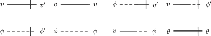
Figure 1: Graphical representation of all propagators of the models given by the quadratic part of the actions (14) and (17).

Graphical representation of propagators is depicted in Fig. 1. Remaining propagators for magnetic admixture and tracer field take the following form, respectively

$$\langle\theta_{i}\theta_{j}^{\prime}\rangle_{0} =\langle\theta_{j}^{\prime}\theta_{i}\rangle_{0}^{*}=\frac{P_{ij}({\bm{k}})}{-{\rm i}\omega+\kappa_{0}k^{2}},$$ (24)

$$\langle\theta\theta^{\prime}\rangle_{0} =\langle\theta^{\prime}\theta\rangle_{0}^{*}=\frac{1}{-{\rm i}\omega+\kappa_{0}k^{2}}.$$ (25)

There are two additional non-zero propagators $\langle\theta_{i}\theta_{j}\rangle_{0}$ and $\langle\theta\theta\rangle_{0}$, but in actual calculations they are in fact not needed [62, 63]. Therefore, we do not quote them here. All the remaining propagators are identically zero, i.e., $\langle\phi^{\prime}\phi^{\prime}\rangle_{0}=\langle v_{i}^{\prime}\phi^{\prime}\rangle_{0}=\langle v_{i}^{\prime}v_{j}^{\prime}\rangle_{0}=\langle\theta_{i}^{\prime}\theta_{j}^{\prime}\rangle_{0}=\langle\theta^{\prime}\theta^{\prime}\rangle_{0}=0$. Self-explanatory graphical representations of non-linearities in studied models together with their vertex factors are depicted in Fig. 2 and Fig. 3.

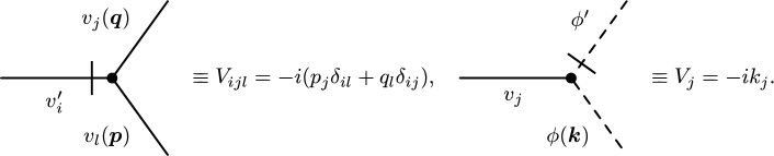
Figure 2: Graphical representation of all interaction vertices of the model related velocity non-linearities of the action (15). For brevity we have retained only those momentum arguments that appear in a resulting vertex factors.

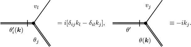
Figure 3: Graphical representation of all interaction vertices of the model given by the advection terms derived from action (16) and action (18), respectively.

Since the theory of critical phenomena corresponds to limit $k\to 0$, in accordance with general theory all the terms in actional functional (and, as a consequence, in propagators) should have the same IR behavior. From the quantity $R$ in Eqs. (23) it follows that $c_{0}^{2}k^{2}\simeq\epsilon_{2}\epsilon_{3}$. This means, that $c_{0}$ is IR significant parameter and, moreover, $c_{0}\simeq k$. Thus, $c_{0}\to 0$ in IR asymptotic and considered model corresponds to large (at least not small as mentioned in [61]) Mach numbers. The situation is typical for processes occuring in the solar corona but not in the atmosphere of the Earth. Note, that this requirement is not connected with calculation scheme which we use (MS scheme, see below) and which allows us to put $c_{0}=0$ in Feynman graphs just as a simplest way to performe calculations and give no restriction for the model. Here, we deal with basic feature of the theory; the situation is analogous to well-known $\varphi^{4}$ model, where parameter $\tau=T-T_{c}$ is IR significant and requirement $\tau\to 0$ near the critical point is in accordance with both physical meaning and requirement of the model. This is the reason why it is impossible to compare our results with previous works [82, 86] where corrections in small Mach numbers to the incompressible case were calculated.

5 Renormalization group analysis

Theoretical models (14) and (17) are amenable to a standard loop expansion using well-known Feynman diagrammatic rules [1, 2]. However, as it is often the case, ordinary perturbation theory is plagued by divergences and these must be properly taken care of. The help comes from renormalization group method, which is considered here in dimensional regularization within minimal subtraction (MS) scheme.

From a practical point of view, theory is renormalized once all 1-particle irreducible Green functions $\Gamma$ (further referred to as 1-irreducible functions) are finite [1, 2]. For dynamical models two independent scales have to be introduced: the time scale $T$ and the length scale $L$. Canonical dimensions of model parameters are found from the requirement that each term of the action functionals (14) and (17) be dimensionless quantity with respect to both the momentum and frequency scales separately. We adopt standard normalization conditions

$$d_{k}^{k}=-d_{x}^{k}=1,\quad d_{k}^{\omega}=d_{x}^{\omega}=0,\quad d_{\omega}^{\omega}=-d_{t}^{\omega}=1,\quad d_{\omega}^{k}=d_{t}^{k}=0.$$ (26)

Then, the overall (total) canonical dimension of any quantity $F$ is described by two numbers, the frequency dimension $d_{F}^{\omega}$ and the momentum dimension $d_{F}^{k}$, and given quantity $F$ therefore scales as $[F]\sim[T]^{-d_{F}^{\omega}}[L]^{-d_{F}^{k}}.$

Based on $d_{F}^{k}$ and $d_{F}^{\omega}$, the total canonical dimension $d_{F}=d_{F}^{k}+2d_{F}^{\omega}$ can be introduced, which in the renormalization theory of dynamic models plays the same role as the conventional (momentum) dimension does in static problems [1, 3]. Assuming quadratic dispersion law $\omega\sim k^{2}$ brought about a scaling relation between time and spatial scale which ensures that all the viscosity and diffusion coefficients in the model are dimensionless.

The canonical dimensions for the velocity part of the model (15) are given in Tab. 1, whereas parameters of the magnetic and tracer part are given in Tab. 2. From Tabs. 1 and 2 it directly follows that the coupling constants $g_{10}\sim[L]^{-y}$ and $g_{20}\sim[L]^{-\varepsilon}$ become simultaneously dimensionless at $y=\varepsilon=0$ what corresponds to the logarithmic theory. Since we use MS scheme the ultraviolet (UV) divergences in the Green functions manifest themselves as poles in $y$, $\varepsilon$ and their linear combinations.

Table 1: Canonical dimensions of the fields and parameters entering field-theoretic action (15) for velocity fluctuations.

$F$	$v_{i}^{\prime}$	$v_{i}$	$\phi^{\prime}$	$\phi$	$\nu_{0}$, $\nu$	$c_{0}$, $c$	$g_{10}$	$g_{20}$	$u_{0}$, $v_{0}$, $u$, $v$, $g_{1}$, $g_{2}$, $\alpha$
$d_{F}^{k}$	$d+1$	$-1$	$d+2$	$-2$	$-2$	$-1$	$y$	$4-d$	0
$d_{F}^{\omega}$	$-1$	1	$-2$	2	1	1	0	0	0
$d_{F}$	$d-1$	1	$d-2$	2	0	1	$y$	$4-d$	0

Table 2: Canonical dimensions of the fields and parameters entering actions  (16) and (18) for advecting fields $\theta_{i}$ (magnetic field) and $\theta$ (tracer field), respectively.

$F$	$\theta_{i}^{\prime},\theta^{\prime}$	$\theta_{i},\theta$	$\kappa$, $\kappa_{0}$	$w_{0}$, $w$
$d_{F}^{k}$	$d$	0	$-2$	0
$d_{F}^{\omega}$	$1/2$	$-1/2$	1	0
$d_{F}$	$d+1$	$-1$	0	0

The total canonical dimension of any 1-irreducible function $\Gamma$ is given by the relation

$$\delta_{\Gamma}=d+2-\sum_{\Phi}N_{\Phi}d_{\Phi},$$ (27)

where $N_{\Phi}$ is the number of the given type of field entering the function $\Gamma$, $d_{\Phi}$ is the corresponding total canonical dimension of field $\Phi$, and the summation runs over all types of the fields $\Phi$ entering the 1-irreducible function $\Gamma$, see [1].

Superficial UV divergences whose removal requires counterterms can be present only in those functions $\Gamma$ for which the formal index of divergence $\delta_{\Gamma}$ is a non-negative integer. A dimensional analysis should be augmented by the several additional considerations. They are summarized in the previous works [62, 63, 74] and we do not repeat them here. The crucial property of studied models is Galilean invariance, whose direct consequence is that fields $v^{\prime}_{i},v_{i},\theta_{i}$ and $\theta$ are not renormalized. Thus, models under considerations with the actions (14) and (17) are renormalizable and the only graphs that are divergent and needed to be considered are two-point Green functions. For a velocity part (15), the following graphs should be analyzed:

$$\raisebox{-4.30554pt}{ \includegraphics[width=81.09052pt]{PhisV2.eps}}\raisebox{-4.30554pt}{ \includegraphics[width=81.09052pt]{PhisV3.eps}}\raisebox{-4.30554pt}{ \includegraphics[width=88.2037pt]{VsVs.eps}}.$$ (28)

For an advected part (vector or tracer field with appropriate changes in propagators and vertices) we have one additional graph:

$$\raisebox{-4.30554pt}{ \includegraphics[width=99.58464pt]{ThTh.eps}}.$$ (29)

Remaining graphs are either UV finite or the Galilean invariance prohibits their appearance. The calculation of the divergent parts of Feynman graphs proceeds in a straightforward fashion and details can be found in [62, 63, 74].

Although, the intermediate steps involved in calculation of the graph presented in (29) differs for vector and tracer cases, the resulting divergent part of the graph is the same and reads

$$D=\frac{\overline{S_{d}}}{2d}p^{2}\nu\biggl{\{}\frac{1-d}{1+w}\biggl{[}\frac{g_{1}}{y}\biggl{(}\frac{\mu}{m}\biggl{)}^{y}+\frac{g_{2}}{\varepsilon}\biggl{(}\frac{\mu}{m}\biggl{)}^{\varepsilon}\biggl{]}{-\frac{u-w}{u(u+w)}\biggl{[}\frac{\alpha g_{1}}{y}\biggl{(}\frac{\mu}{m}\biggl{)}^{y}+\frac{g_{2}}{\varepsilon}\biggl{(}\frac{\mu}{m}\biggl{)}^{\varepsilon}\biggl{]}\biggl{\}}},$$ (30)

where $\overline{S_{d}}=S_{d}/(2\pi)^{d}$ with $S_{d}=2\pi^{d/2}/\Gamma(d/2)$ being the surface area of the unit sphere in the $d$-dimensional space; $\Gamma(x)$ is Euler’s Gamma function. Parameter $\mu$ is a renormalization mass employed in minimal subtraction scheme [1, 3]. For vector admixture expression (30) should be multiplied by a projection operator $P_{ij}({\bm{p}})$ due to a vector nature of magnetic field $\theta_{i}$.

From the result (30) we easily derive renormalization constant $Z_{\kappa}$ for the parameter $\kappa$ related to the advected fields [see Eq. (16)] and the anomalous dimension $\gamma_{\kappa}$:

$$Z_{\kappa} =1-\frac{g_{1}}{2dwy}\biggl{[}\frac{d-1}{1+w}+\frac{\alpha(u-w)}{u(u+w)^{2}}\biggl{]}-\frac{g_{2}}{2dw\varepsilon}\biggl{[}\frac{d-1}{1+w}+\frac{(u-w)}{u(u+w)^{2}}\biggl{]},$$ (31)

$$\gamma_{\kappa} =\frac{g_{1}}{2dw}\biggl{[}\frac{d-1}{1+w}+\frac{\alpha(u-w)}{u(u+w)^{2}}\biggl{]}+\frac{g_{2}}{2dw}\biggl{[}\frac{d-1}{1+w}+\frac{(u-w)}{u(u+w)^{2}}\biggl{]}.$$ (32)

6 Scaling regimes

Underlying idea of RG approach [1, 2, 3] is embodied in a relation between the initial and renormalized action functionals $\mathcal{S}(\Phi,e_{0})=\mathcal{S}_{R}(Z_{\Phi}\Phi,e,\mu)$, where $e_{0}$ denotes the complete set of bare parameters, $e$ is the set of their renormalized counterparts, and $\Phi$ stands for a complete set of fields $\{\varphi\}$ and their response counterparts $\{\varphi^{\prime}\}$. This relation can be converted into a differential form

$$\biggl{\{}{\cal D}_{RG}+N_{\varphi}\gamma_{\varphi}+N_{\varphi^{\prime}}\gamma_{\varphi^{\prime}}\biggr{\}}\,G^{R}(e,\mu,\dots)=0,$$ (33)

where $G=\langle\Phi\cdots\Phi\rangle$ is an arbitrary Green function of the theory; $N_{\varphi}$ and $N_{\varphi^{\prime}}$ are the numbers of entering fields $\varphi$ and $\varphi^{\prime}$ in $G$, the ellipsis commonly denotes remaining arguments of $G$ (such as spatial and time variables), ${\cal D}_{RG}$ is the operation $\widetilde{\cal D}_{\mu}$ expressed in the renormalized variables, and $\widetilde{\cal D}_{\mu}$ is the differential operation $\mu\partial_{\mu}$ at fixed bare parameters $e_{0}$. For the present model it takes the form

$${\cal D}_{RG}={\cal D}_{\mu}+\sum\beta_{g}\partial_{g}-\gamma_{\nu}{\cal D}_{\nu}-\gamma_{c}{\cal D}_{c},$$ (34)

where the sum runs over the set of all charges $\{g_{1},g_{2},u,v,w\}$, $\nu$ and $c$ are viscosity and adiabatic speed of sound, respectively, and differential operator ${\cal D}_{x}=x\partial_{x}$ has been introduced. The $\gamma$ and $\beta$-functions are defined as $\gamma_{F}=\widetilde{\cal D}_{\mu}\ln Z_{F}$ and $\beta_{g}=\widetilde{\cal D}_{\mu}g$. The latter ones can be expressed in terms of anomalous dimensions:

$$\beta_{g_{1}}=g_{1}\,(-y-\gamma_{g_{1}}),\,\beta_{g_{2}}=g_{2}\,(-\varepsilon-\gamma_{g_{2}}),\,\beta_{u}=-u\gamma_{u},\,\beta_{v}=-v\gamma_{v},\,\beta_{w}=w(\gamma_{\nu}-\gamma_{\kappa}).$$ (35)

The last expression follows from the introduced definition of the charge $w$ in Eq. (16).

Macroscopic scaling regimes are naturally identified with the IR attractive (“stable”) fixed points $g^{*}\equiv\{g_{1}^{*},g_{2}^{*},u^{*},v^{*},w^{*}\}$, whose coordinates are found from the conditions [1, 3]

$$\beta_{g_{1}}(g^{*})=\beta_{g_{2}}(g^{*})=\beta_{u}(g^{*})=\beta_{v}(g^{*})=\beta_{w}(g^{*})=0.$$ (36)

This statement is a direct consequence of the invariant couplings behavior. Let us consider a set of invariant couplings $\overline{g}_{i}=\overline{g}_{i}(s,g)$ with the initial data $\overline{g}_{i}|_{s=1}=g_{i}$, where $s=k/\mu$. IR (macroscopic) asymptotic behavior is obtained in the limit $s\rightarrow 0$. An evolution of invariant couplings satisfies flow equations $\mathcal{D}_{s}\overline{g}_{i}=\beta_{i}(\overline{g}_{j}),$ and in a limit $s\to 0$ it can be approximated as $\overline{g}_{i}(s,g^{*})\cong g^{*}+const\times s^{\omega_{i}}.$ A set $\{\omega_{i}\}$ contains all eigenvalues of the matrix

$$\Omega_{ij}=\partial\beta_{i}/\partial g_{j}|_{g=g_{*}}.$$ (37)

The existence of IR attractive solutions of the RG equations corresponds to such fixed points for which the matrix (37) is positive definite. These fixed points are then natural candidates for macroscopically observable scaling regimes.

In the double expansion approach we have used, the character of the IR behavior depends on the mutual relation between $y$ and $\varepsilon$. In work [74] the velocity part of the system (35), which don’t include $\beta_{w}$, was thoroughly analyzed. The net result of the analysis is a prediction of three IR attractive fixed points. The fixed point FPI (the trivial or Gaussian point) is stable if $y$, $\varepsilon<0$ and has the coordinates

$$g_{1}^{*}=0,\quad g_{2}^{*}=0,\quad\text{both}\ u^{*}\ \text{and}\ v^{*}\ \text{are arbitrary}.$$ (38)

The fixed point FPII, which is stable if $\varepsilon>0$ and $y<3\varepsilon/2$, has the coordinates

$$g_{1}^{*}=0,\quad g_{2}^{*}=\frac{8\varepsilon}{3},\quad u^{*}=v^{*}=1.$$ (39)

The fixed point FPIII, which is stable if $y>0$ and $y>3\varepsilon/2$, has the coordinates

$$g_{1}^{*}=\frac{16y(2y-3\varepsilon)}{9[y(2+\alpha)-3\varepsilon]},\quad g_{2}^{*}=\frac{16\alpha y^{2}}{9[y(2+\alpha)-3\varepsilon]},\quad u^{*}=v^{*}=1.$$ (40)

The crossover between the two nontrivial points (39) and (40) takes place across the line $y=3\varepsilon/2$, which is in accordance with results of [53].

Substituting obtained values of $u^{*}$ and $v^{*}$ together with $d=4$ we obtain for the charge $w$ the following beta function

$$\beta_{w}=\frac{w-1}{16w(1+w)^{2}}\biggl{[}g_{1}(6+2\alpha+9w+3w^{2})+g_{2}(3w^{2}+9w+8)\biggl{]}.$$ (41)

Note that this result agrees with previous works for the passive scalar case [74] and vector case [87] as well. The expression in the square brackets in Eq. (41) is always positive for physically permissible values $g_{1}>0,g_{2}>0,w>0$ and $\alpha>0$. Therefore, only one nontrivial solution for the fixed point $w^{*}=1$ exists. It is straightforward to prove that $\partial_{w}\beta_{w}>0$ for nontrivial fixed points FPII and FPIII, which ensures IR stability with respect to $w$ charge. Once scaling regimes are found, the critical dimensions for various quantities $F$ can be calculated via the relation

$$\Delta[F]=d^{k}_{F}+\Delta_{\omega}d^{\omega}_{F}+\gamma_{F}^{*},$$ (42)

where $d^{\omega}_{F}$ is the canonical frequency dimension, $d^{k}_{F}$ is the momentum dimension, $\gamma_{F}^{*}$ is the anomalous dimension at the fixed point (FPII or FPIII), and $\Delta_{\omega}=2-\gamma_{\nu}^{*}$ is the critical dimension of frequency. Using Eq. (42) the critical dimensions of advected fields are obtained for the fixed points FPII and FPIII:

$$\Delta_{\theta_{i}} =-1+\varepsilon/4,\quad\Delta_{\theta_{i}^{\prime}}=d+1-\varepsilon/4\quad\text{for FP${\textrm{II}}$},$$ (43)

$$\Delta_{\theta_{i}} =-1+y/6,\quad\Delta_{\theta_{i}^{\prime}}=d+1-y/6\quad\text{for FP${\textrm{III}}$}.$$ (44)

7 Composite Fields

From experimental point of view much more relevant than critical dimensions are quantities known as correlation and structure functions. In field-theoretic framework they are usually represented by certain composite operators. A local composite operator is a monomial or polynomial constructed from the primary fields and their finite-order derivatives at a single space-time point. In the Green functions with such objects, new UV divergences arise due to the coincidence of the field arguments. Their removal requires an additional renormalization procedure [1, 3].

It is not common to consider in one paper both tracer and vector admixtures. The reason is that the expressions for tracer case are completely analogous to the vector ones in the part connected with composite fields $\theta$ and can be easily obtained by considering operator $\partial_{i}\theta$ instead of $\theta_{i}$ in all formulas quoted below (note, that propagators (24), (25) and vertices depicted in Fig. 3 still differs for tracer and vector cases). This is a consequence of the fact that instead of density case for tracer admixture the operators $\theta^{n}$ are UV finite and, therefore, we should consider operators $\partial_{i}\theta$ which contain derivatives. This is why both density and tracer are scalar fields, but yield different expressions. Moreover, consideration of tracer field is much more closer to the vector case rather to the density one.

For brevity, hereinafter we write all expressions related to operators $\theta_{i}$ or $\partial_{i}\theta$ (for vector or tracer cases, respectively) below only for the vector case and use notation $\theta_{i}$ for vector field. In the case of vector admixture we should focus on the irreducible tensor operators of the form

$$F^{(n,l)}_{i_{1}\dots i_{l}}=\theta_{i_{1}}\cdots\theta_{i_{l}}\,(\theta_{j}\theta_{j})^{s}+\dots,$$ (45)

where $l$ is the number of the free vector indices (the rank of the tensor) and $n=l+2s$ is the total number of the fields $\theta_{i}$ entering the operator. The ellipsis stands for the subtractions with the Kronecker’s delta symbols that make the operator irreducible (so that a contraction with respect to any pair of the free tensor indices vanish). For instance,

$$F^{(2,2)}_{ij}=\theta_{i}\theta_{j}-\frac{\delta_{ij}}{d}\,(\theta_{k}\theta_{k}).$$ (46)

For a theoretical analysis, it is convenient to contract the tensors (45) with an arbitrary constant vector $\lambda$$=\{\lambda_{i}\}$. The resulting scalar operator then takes the form

$$F^{nl}=(\lambda_{i}w_{i})^{l}(w_{i}w_{i})^{s}+\dots,\quad w_{i}\equiv\theta_{i},$$ (47)

where the subtractions, denoted by the ellipsis, necessarily contain factors of $\lambda^{2}=\lambda_{i}\lambda_{i}$.

In order to calculate the critical dimension of an operator, we have to renormalize it. The operators (45) can be treated as multiplicatively renormalizable, $F^{nl}=Z_{nl}F^{nl}_{R}$, with certain renormalization constants $Z_{(n,l)}$ [62, 63]. The counterterm to $F^{nl}$ must have the same rank as the operator itself. It means that the terms containing $\lambda^{2}$ should be excluded since the contracted fields $w_{i}w_{i}$, which naturally appear in such terms, reduce the number of free indices. The renormalization constants $Z_{nl}$ are determined by the finiteness of the 1-irreducible Green function $\Gamma_{nl}(x;\theta)$, where $x=(t,{\bm{x}})$ is a functional argument of the operator $\theta$. In the one-loop approximation we have a diagrammatic equation

$$\Gamma_{nl}(x;\theta)=F^{nl}+\frac{1}{2}\raisebox{-17.22217pt}{ \includegraphics[width=34.14322pt]{comp.eps}},$$ (48)

where numerical factor $1/2$ is a symmetry factor of the graph. The thick dot in the top of the graph represents the operator vertex, which up to irrelevant terms can be presented in the form

$$V(x;x_{1},x_{2})=\frac{\partial^{2}F^{nl}}{\partial w_{i}\partial w_{j}}\,\delta(x-x_{1})\,\delta(x-x_{2}).$$ (49)

The differentiation yields

$${\partial^{2}F^{nl}}/{\partial w_{i}\partial w_{j}} =2s(w^{2})^{s-2}(\lambda w)^{l}\left[\delta_{ij}w^{2}+2(s-1)w_{i}w_{j}\right]+l(l-1)(w^{2})^{s}$$

$$\times(\lambda w)^{l-2}\lambda_{i}\lambda_{j}+2ls(w^{2})^{s-1}(\lambda w)^{l-1}(w_{i}\lambda_{j}+w_{j}\lambda_{i}),$$ (50)

where $w^{2}=w_{k}w_{k}$, $(\lambda w)=\lambda_{k}w_{k}$ and substitution $w_{i}\rightarrow\theta_{i}$ is assumed. Two more factors $w_{p}w_{r}$ are attached to the bottom of the graph due to the derivatives stemming from the vertices $\theta^{\prime}_{i}(v_{k}\partial_{k})\theta_{i}$.

The UV divergence is logarithmic and one can set all the external frequencies and momenta equal to zero. Since propagators (24), (25) and vertices depicted in Fig. 3 are different for vector and tracer cases, the core of the graph also differs for these two cases. For tracer field it reads

$$\widehat{D}_{ij}^{pr}=\int\frac{\text{d}\omega}{2\pi}\int\displaylimits_{k>m}\frac{{{\mathrm{d}}^{d}}{k}}{(2\pi)^{d}}\,k_{i}k_{j}\,D^{v}_{pr}(\omega,{{\bm{k}}})\,\frac{1}{\omega^{2}+w^{2}\nu^{2}k^{4}}.$$ (51)

Here, the first factor comes from the derivatives in (50), $D^{v}_{pr}$ is the velocity correlation function [see Eq. (5)], and the last factor comes from the two propagators $\langle\theta^{\prime}_{i}\theta_{j}\rangle_{0}$. The indices $i$ and $j$ should be later contracted with expression (50), the indices $p$ and $r$ with external fields $w_{p}$ and $w_{r}$ denoted by “legs” of the graph.

For vector field the core of the graph takes the form

$$\widetilde{D}_{ij}^{xy}=\int\frac{\text{d}\omega}{2\pi}\int\displaylimits_{k>m}\frac{{{\mathrm{d}}^{d}}{k}}{(2\pi)^{d}}\,P_{ai}(\bm{k})P_{bj}(\bm{k})\,D^{v}_{pr}(\omega,{{\bm{k}}})\,\frac{1}{\omega^{2}+w^{2}\nu^{2}k^{4}}V_{apx}(\bm{k})V_{bry}(\bm{k}),$$ (52)

where $P_{ai}(\bm{k})$ and $P_{bj}(\bm{k})$ follows from propagators (25), $V_{apx}(\bm{k})$ and $V_{bry}(\bm{k})$ are two vector vertices (see Fig. 3), and $D^{v}_{pr}$ is the velocity correlation function. For brevity we do not draw here picture for the graph with explicitly written vector indices, but they may be easily restored from the above written expression.

After the integration, combining all the factors, contracting the tensor indices and expressing the result in terms of $n=l+2s$ and $l$, one obtains

$$=-\frac{F_{nl}}{2wd(d+2)}\biggl{[}\frac{Q_{1}}{(1+w)}\biggl{(}\frac{g_{1}}{y}+\frac{g_{2}}{\varepsilon}\biggl{)}+\frac{Q_{2}}{u(u+w)}\biggl{(}\frac{\alpha g_{1}}{y}+\frac{g_{2}}{\varepsilon}\biggl{)}\biggl{]},$$ (53)

where

$$Q_{1} =-n(n+d)(d-1)+l(d+1)(d+l-2),$$

$$Q_{2} =-n(3n+d-4)+l(d+l-2)$$ (54)

for tracer case and

$$Q_{1} =-n(n+d)(d-1)+l(d+1)(d+l-2),$$

$$Q_{2} =-n(n+nd-d)(d-1)+l(d+l-2)$$ (55)

for vector case. Finally, expression (48) reads

$$\Gamma_{nl}(x;\theta)=F^{nl}(x)\,\biggl{\{}1-\frac{1}{4wd(d+2)}\,\biggl{[}\frac{Q_{1}}{(1+w)}\biggl{(}\frac{g_{1}}{y}+\frac{g_{2}}{\varepsilon}\biggl{)}+\frac{Q_{2}}{u(u+w)}\biggl{(}\frac{\alpha g_{1}}{y}+\frac{g_{2}}{\varepsilon}\biggl{)}\biggl{]}\biggl{\}}.$$ (56)

The renormalization constants $Z_{nl}$ calculated in the MS scheme thus take the form

$$Z_{nl}=1-\frac{1}{4dw(d+2)}\,\left[\frac{Q_{1}}{1+w}\left(\frac{g_{1}}{y}+\frac{g_{2}}{\varepsilon}\right)+\frac{Q_{2}}{u(u+w)}\left(\frac{\alpha g_{1}}{y}+\frac{g_{2}}{\varepsilon}\right)\right]$$ (57)

and for the corresponding anomalous dimensions we get

$$\gamma_{nl}=\frac{1}{4dw(d+2)}\,\left\{\frac{Q_{1}}{1+w}(g_{1}+g_{2})+\frac{Q_{2}}{u(u+w)}(\alpha g_{1}+g_{2})\right\}.$$ (58)

Now in order to evaluate the critical dimensions of the operators $F_{nl}$ one needs to substitute the coordinates of the fixed points into the expression (58) and then use the relation (42). For the fixed point FPII the critical dimension is

$$\Delta_{nl}=\frac{n}{4}\varepsilon+\frac{Q_{1}+Q_{2}}{72}\varepsilon;$$ (59)

for the fixed point FPIII it is

$$\Delta_{nl}=\frac{n}{6}y+\frac{y}{12}\frac{Q_{1}(\alpha y+2y-3\varepsilon)+3\alpha Q_{2}(y-\varepsilon)}{9[y(2+\alpha)-3\varepsilon]}.$$ (60)

Both expressions (59) and (60) might be affected by higher order corrections in $y$ and $\varepsilon$. Inspection of expressions (59) and (60) reveals that increasing value of $n$ leads to a infinite set of operators with negative critical dimensions. Their spectra are unbounded from below, see Appendix A in [63].

The latter result for FPIII is in accordance with previously known results [62, 63] for the analysis near three-dimensional space $d=3$:

$$\Delta_{nl} =\frac{ny}{6}+\frac{y(Q_{1}+\alpha Q_{2})}{6(d-1)(d+2)},$$ (61)

where $Q_{1}$ and $Q_{2}$ coincide with those given in Eqs. (54) and (55) for tracer and vector cases, respectively. Expression (61) at $d=4$ reads

$$\big{.}\Delta_{nl}\biggl{|}_{d=4} =\frac{ny}{6}+\frac{y(Q_{1}+\alpha Q_{2})}{108}.$$ (62)

Expanding the expression (60) in $y$ at fixed value $\varepsilon=1$ (which corresponds to $d=3$) yields

$$\Delta_{nl} =\frac{ny}{6}+\frac{y(Q_{1}+\alpha Q_{2})}{108}+\mathcal{O}(y^{2}).$$ (63)

From the expressions (62) and (63) it follows that the expression (60), obtained as a result of the double $y$ and $\varepsilon$ expansion near $d=4$, may be considered as a certain partial infinite resummation of the ordinary $y$ expansion. This resummation significantly improves the situation at large $\alpha$: now we do not have the pathology when the critical dimensions $\Delta_{nl}$ are linear in $\alpha$ and, therefore, grow with $\alpha$ without a bound.

8 Operator Product Expansion

Our main interest are pair correlation functions constructed from the composite operators, whose unrenormalized counterparts have been defined in Eq. (45). For Galilean invariant equal-time functions we can write the representation

$$\langle F^{mi}(t,{\bm{x}})F^{nj}(t,{\bm{x}}^{\prime})\rangle\simeq\mu^{d_{F}}\nu^{d^{\omega}_{F}}(\mu r)^{-\Delta_{mi}-\Delta_{nj}}\zeta_{mi;nj}(mr,c(r)),$$ (64)

where $r=|{\bm{x}}-{\bm{x}}^{\prime}|$ and $c(r)$ is effective speed of sound. Its limiting behavior is

$$c(r)=c\frac{(\mu r)^{\Delta_{c}}}{\mu\nu}\rightarrow\begin{cases}c(0)\quad\text{{for} non-local regime FPIII};\\ c(\infty)\quad\text{{for} local regime FPII},\end{cases}$$ (65)

see [74].

Expression (64) is valid in the asymptotic limit $\mu r\gg 1$. Further, the inertial-convective range corresponds to the additional restriction $mr\ll 1$. The behavior of the functions $\zeta$ at $mr\to 0$ can be studied by means of the OPE technique [1, 3]. The basic idea of this method is to represent a product of two operators at two close points ${\bm{x}}$ and ${\bm{x}}^{\prime}$ with a condition ${\bm{x}}-{\bm{x}}^{\prime}\rightarrow 0$ in the form

$$F^{mi}(t,{\bm{x}})F^{nj}(t,{\bm{x}}^{\prime})\simeq\sum_{F}C_{F}(mr)\,F\biggl{(}t,\frac{{\bm{x}}+{\bm{x}}^{\prime}}{2}\biggl{)},$$ (66)

where functions $C_{F}$ are regular in their arguments and a given sum runs over all permissible local composite operators $F$ allowed by RG and symmetry considerations. Taken into account (64) and (66) in the limit $mr\rightarrow 0$ we arrive at the relation

$$\zeta(mr)\simeq\sum_{F}A_{F}(mr)(mr)^{\Delta_{F}}.$$ (67)

Singularities for $mr\to 0$ (and thus the anomalous scaling) result from the contributions in (67) of the operators with negative critical dimensions, see Eqs. (59) and (60).

Considering OPE for the correlation functions $\langle F^{(p,0)}F^{(k,0)}\rangle$ constructed from scalar operators of the type (45), one can observe that the leading contribution to the expansion is determined by the operator $F^{(n,0)}$ with $n=p+k$ from the same family. Therefore, in the inertial range these correlation functions acquire the form

$$\langle F^{(p,0)}(t,{{\bm{x}}})F^{(k,0)}(t,{{\bm{x}}^{\prime}})\rangle\sim r^{-\Delta_{p0}-\Delta_{k0}+\Delta_{n0}}.$$ (68)

The inequality $\Delta_{n0}<\Delta_{p0}+\Delta_{k0}$, which follows from both explicit one-loop expressions (59) and (60), indicates, that the operators $F^{(n,0)}$ demonstrate a multifractal behavior for both regimes FPII and FPIII; see [88, 89].

A direct substitution of $d=4$ leads to the following prediction for a critical dimensions

$$\Delta_{nl}=n\Delta_{\theta}+\gamma^{*}_{nl}=\begin{cases}-n+\frac{n\varepsilon}{4}+\frac{(Q_{1}+Q_{2})\varepsilon}{4}\qquad\mbox{ }\hskip 45.52458pt\text{for FPII},\\ -n+\frac{ny}{6}+\frac{Q_{1}y}{108}+\frac{Q_{2}\alpha y(y-\varepsilon)}{36[y(2+\alpha)-3\varepsilon]}\qquad\text{for FPIII},\end{cases}$$ (69)

where we have

$$Q_{1}|_{d=4}=-3n(n+4)+5l(l+2),\quad Q_{2}|_{d=4}=-3n^{2}+l(l+2)$$ (70)

for tracer case and

$$Q_{1}|_{d=4}=-3n(n+4)+5l(l+2),\quad Q_{2}|_{d=4}=-3n(5n-4)+l(l+2)$$ (71)

for vector case. From Eq. (69) and Eqs. (70), (71) it follows that for fixed $n$ a kind of an hierarchy present with respect to the index $l$, which measures the “degree of anisotropy:”

$$\frac{\partial\Delta_{nl}}{\partial l}>0.$$ (72)

In other words, the higher $l$ the less important contribution. The most relevant is given by the isotropic shell with $l=0$. This is in accordance with previous studies [62, 63, 87] and hypothesis about restoration of isotropy and symmetries of turbulent motion in the statistical sence in the depth of inertial interval [90].

9 Conclusion

In the present paper the advection problem of the vector and tracer field by the Navier-Stokes velocity ensemble have been examined. The fluid was assumed to be compressible and the space dimension was close to $d=4$. This specific case allows us to take into consideration one more divergent function, namely $\left\langle v^{\prime}v^{\prime}\right\rangle_{\text{1-ir}}$, and construct the double expansion in $y$ and $\varepsilon=4-d$. This leads to richer results in comparison with naive consideration of the system near physical dimension $d=3$.

Using renormalization group technique two nontrivial IR stable fixed points were identified and, therefore, the critical behavior in the inertial range demonstrates two different nontrivial regimes depending on the relation between the exponents $y$ and $\varepsilon$. The expressions for the critical exponents of the advected fields $\theta$ were obtained in the leading one-loop approximation.

In order to find the anomalous exponents of the structure functions, the composite fields (45) were renormalized. The critical dimensions of them were evaluated. Moreover, operator product expansion allowed us to derive the explicit expressions for the critical dimensions of the structure functions.

The existence of the anomalous scaling (singular power-like dependence on the integral scale $L$) in the inertial-convective range was established for both possible scaling regimes. From the leading order (one-loop) calculations it follows that the main contribution into the OPE is given by the isotropic term corresponding to $l=0$, where $l$ is the rank of the tensor and serves as a degree of the anisotropy; all other terms with $l\geq 2$ provide only corrections. These facts give a quantitative illustration of the general concept that the symmetries of the Navier-Stokes equation, broken spontaneously and by initial or boundary conditions, are restored in the statistical sense for the fully developed turbulence [4, 5, 6]. Another very interesting result is that correlations of the advected fields exhibit multifractal behavior.

The results of this study are especially significant at large values of $\alpha$ (purely potential random force). In contrast to analysis near $d=3$, in the present case the anomalous dimensions of the composite operators (59) and (60) do not grow with $\alpha$ without a bound. This is a consequence of eliminating the poles in $\varepsilon$ near $d=4$, which leads to a significant improvement of calculated expressions for critical dimensions near physical value $d=3$. Expression (60) obtained in this study may be considered as an example of infinite resummation of ordinary $y$ expansion. It works well at large $\alpha$ being not expanded in $y$, and the first term of this expansion coincides with the answer presented earlier in [63]; see expressions (62) – (63).

Regarding future tasks, it would be interesting to go beyond the one-loop approximation and to analyze the behavior more accurately. Another very important issue to be further investigated is to have a closer look at the both scalar and vector active fields, i.e., to consider a back influence of the advected fields to the turbulent environment flow.

References

- [1] A. N. Vasil’ev, The Field Theoretic Renormalization Group in Critical Behavior Theory and Stochastic Dynamics (Boca Raton, Chapman Hall/CRC, 2004).
- [2] U. Täuber, Critical Dynamics: A Field Theory Approach to Equilibrium and Non-Equilibrium Scaling Behavior (Cambridge University Press, New York, 2014).
- [3] J. Zinn-Justin, Quantum Field Theory and Critical Phenomena (4th edition, Oxford University Press, Oxford, 2002).
- [4] U. Frisch, Turbulence: The Legacy of A. N. Kolmogorov (Cambridge University Press, Cambridge, 1995).
- [5] A. S. Monin, A. M. Yaglom, Statistical Fluid Mechanics:Vol 2 (MIT Press, Cambridge, 1975).
- [6] P. A. Davidson, Turbulence: an introduction for scientists and engineers (2th edition, Oxford University Press, Oxford, 2015).
- [7] G. Falkovich, K. Gawȩdzki and M. Vergassola, Rev. Mod. Phys. 73, 913 (2001).
- [8] D. Biskamp, Magnetohydrodynamic Turbulence (Cambridge Univ. Press, Cambridge, 2003).
- [9] S. N. Shore, Astrophysical Hydrodynamics:An Introduction (Wiley-VCH Verlag GmbH& KGaA, Weinheim, 2007).
- [10] E. Priest, Magnetohydrodynamics of the sun (Cambridge University Press, 2014).
- [11] A. Pouquet, U. Frisch, J. Léorat, J. Fluid Mech. 77, 321 (1976).
- [12] C.-Y. Tu, E. Marsch, Space Sci. Rev. 73, 1 (1995).
- [13] S. A. Balbus, J. F. Hawley, Rev. Mod. Phys. 70, 1 (1998).
- [14] G. Chabrier, Publ. Astron. Soc. Pac. 115, 763 (2003).
- [15] B. G. Elemegreen, J. Scalo, Annu. Rev. Astron. Astrophys. 42, 211 (2004).
- [16] C. Federrath, Mon. Notices Royal Astron. Soc. 436, 1245 (2013).
- [17] N. V. Antonov, J. Phys. A: Math. Gen. 39, 7825 (2006).
- [18] H. K. Moffatt, Magnetic field generation in electrically conducting fluids (Cambridge University Press, Cambridge 1978).
- [19] J. D. Fournier, P. L. Sulem, A. Pouquet, J. Phys. A 15, 1393 (1982).
- [20] L. Ts. Adzhemyan, A. N. Vasil’ev, and M. Gnatich, Theor. Math. Phys. 64(2), 777 (1985).
- [21] L. D. Landau and E. M. Lifshitz, Fluid Mechanics (Pergamon Press, Oxford, 1959).
- [22] P. Sagaut, C. Cambon, Homogeneous Turbulence Dynamics (Cambridge University Press, 2008).
- [23] J. Kim, and D. Ryu, Astrophys. J. 630, L45 (2005).
- [24] V. Carbone, R. Marino, L. Sorriso-Valvo, A. Noullez, and R. Bruno, Phys. Rev. Lett. 103, 061102 (2009).
- [25] F. Sahraoui, M. L. Goldstein, P. Robert, Yu. V. Khotyainstsev, Phys. Rev. Lett. 102, 231102 (2009).
- [26] H. Aluie, and G. L. Eyink, Phys. Rev. Lett. 104, 081101 (2010).
- [27] S. Galtier, and S. Banerjee, Phys. Rev. Lett. 107, 134501 (2011).
- [28] S. Banerjee, and S. Galtier, Phys. Rev. E 87, 013019 (2013).
- [29] S. Banerjee, L. Z. Hadid, F. Sahraoui, and S. Galtier, Astrophys. J. Lett. 829, L27, (2016).
- [30] L. Z. Hadid, F. Sahraoui, and S. Galtier, Astrophys. J. 838, 9 (2017).
- [31] P. S. Iroshnikov, Sov. Astron. 7, 566 (1964).
- [32] N. V. Antonov and N. M. Gulitskiy, Lecture Notes in Comp. Science, 7125/2012, 128 (2012).
- [33] N. V. Antonov and N. M. Gulitskiy, Phys. Rev. E 85, 065301(R) (2012).
- [34] N. V. Antonov and N. M. Gulitskiy, Phys. Rev. E 87, 039902(E) (2013).
- [35] E. Jurčišinova and M. Jurčišin, J. Phys. A: Math. Theor., 45, 485501 (2012).
- [36] E. Jurčišinova and M. Jurčišin, Phys. Rev. E 77, 016306 (2008).
- [37] E. Jurčišinova, M. Jurčišin and R. Remecky, Phys. Rev. E 80, 046302 (2009).
- [38] N. V. Antonov and N. M. Gulitskiy, Phys. Rev. E 91, 013002 (2015).
- [39] N. V. Antonov and N. M. Gulitskiy, Phys. Rev. E 92, 043018 (2015).
- [40] N. V. Antonov and N. M. Gulitskiy, AIP Conf. Proc. 1701, 100006 (2016).
- [41] N. V. Antonov and N. M. Gulitskiy, EPJ Web of Conf. 108, 02008 (2016).
- [42] L. Ts. Adzhemyan, N. V. Antonov, A. N. Vasil’ev: The Field Theoretic Renormalization Group in Fully Developed Turbulence (Gordon & Breach, London, 1999).
- [43] R.H. Kraichnan, Phys. Fluids 11, 945 (1968).
-
[44]
K. Gawȩdzki and A. Kupiainen, Phys. Rev. Lett. 75, 3834 (1995);
D. Bernard, K. Gawȩdzki, and A. Kupiainen, Phys. Rev. E 54, 2564 (1996);
M. Chertkov and G. Falkovich, Phys. Rev. Lett. 76, 2706 (1996) - [45] L. Ts. Adzhemyan, N. V. Antonov, and A. N. Vasil’ev, Phys. Rev. E 58, 1823 (1998).
- [46] N. V. Antonov, Phys. Rev. E 60, 6691 (1999).
- [47] E. Jurčišinova and M. Jurčišin, Phys. Rev. E 91, 063009 (2015).
-
[48]
N. V. Antonov, A. Lanotte, and A. Mazzino, Phys. Rev. E 61, 6586 (2000);
N. V. Antonov and N. M. Gulitskiy, Theor. Math. Phys., 176(1), 851 (2013). - [49] H. Arponen, Phys. Rev. E, 79, 056303 (2009).
- [50] E. Jurčišinova, M. Jurčišin, M. Menkyna, EPJ B 91, 313 (2018).
- [51] M. Hnatič, J. Honkonen, T. Lučivjanský, Acta Physica Slovaca 66, 69 (2016).
- [52] L. Ts. Adzhemyan, N. V. Antonov, J. Honkonen, and T. L. Kim, Phys. Rev. E 71, 016303 (2005).
- [53] N. V. Antonov, Phys. Rev. Lett. 92, 161101 (2004).
- [54] N. V. Antonov, N. M. Gulitskiy, and A. V. Malyshev, EPJ Web of Conf. 126, 04019 (2016).
- [55] E. Jurčišinova, M. Jurčišin, R. Remecky, Phys. Rev. E 93, 033106 (2016).
- [56] E. Jurčišinova, M. Jurčišin, M. Menkyna, Phys. Rev. E 95, 053210 (2017).
- [57] M. Vergassola and A. Mazzino, Phys. Rev. Lett. 79, 1849 (1997).
- [58] A. Celani, A. Lanotte, and A. Mazzino, Phys. Rev. E 60 R1138 (1999).
- [59] M. Chertkov, I. Kolokolov, and M. Vergassola, Phys. Rev. E. 56, 5483 (1997).
- [60] L. Ts. Adzhemyan, N. V. Antonov, Phys. Rev. E 58, 7381 (1998).
- [61] N. V. Antonov, M. Yu. Nalimov and A. A. Udalov, Theor. Math. Phys. 110, 305 (1997).
- [62] N. V. Antonov and M. M. Kostenko, Phys. Rev. E 90, 063016 (2014).
- [63] N. V. Antonov and M. M. Kostenko, Phys. Rev. E 92, 053013 (2015).
- [64] M. Hnatich, E. Jurčišinova, M. Jurčišin, and M. Repašan, J. Phys. A: Math. Gen. 39, 8007 (2006).
- [65] V. S. L’vov and A. V. Mikhailov, Preprint No. 54, Inst. Avtomat. Electron., Novosibirsk (1977).
- [66] I. Staroselsky, V. Yakhot, S. Kida, and S. A. Orszag, Phys. Rev. Lett., 65, 171 (1990).
- [67] S. S. Moiseev, A. V. Tur, and V. V. Yanovskii, Sov. Phys. JETP 44, 556 (1976).
- [68] J. Honkonen and M. Yu. Nalimov, Z. Phys. B 99, 297 (1996).
- [69] L. Ts. Adzhemyan, J. Honkonen, M. V. Kompaniets, A. N. Vasil’ev, Phys. Rev. E 71(3), 036305 (2005).
- [70] L. Ts. Adzhemyan, M. Hnatich and J. Honkonen, Eur. Phys. J B 73, 275 (2010).
- [71] A. Z. Patashinskii, V. L. Pokrovskii, Fluctuation Theory of Phase Transitions (Pergamon Press, Oxford, 1979).
- [72] D. Forster, D. R. Nelson, M. J. Stephen, Phys. Rev. A 16, 732 (1977).
- [73] L. Ts. Adzhemyan, N. V. Antonov, and A. N. Vasil’ev, Sov. Phys. JETP 68, 733 (1989).
- [74] N.V. Antonov, N. M. Gulitskiy, M. M. Kostenko, T. Lučivjanský, Phys. Rev. E 95, 033120 (2017).
- [75] N.V. Antonov, N. M. Gulitskiy, M. M. Kostenko, T. Lučivjanský, EPJ Web of Conf. 125, 05006 (2016).
- [76] N.V. Antonov, N. M. Gulitskiy, M. M. Kostenko, T. Lučivjanský, EPJ Web of Conf. 137, 10003 (2017).
- [77] N.V. Antonov, N. M. Gulitskiy, M. M. Kostenko, T. Lučivjanský, EPJ Web of Conf. 164, 07044 (2017).
- [78] N. V. Antonov, A. Lanotte, and A. Mazzino, Phys. Rev. E 61, 6586 (2000).
- [79] Ye Zhou, Phys. Rep. 448, 1 (2010).
- [80] M. K. Nandy and J. K. Bhattacharjee, J. Phys. A: Math. Gen., 31, 2621 (1998).
- [81] N. V. Antonov, Physica D 144, 370 (2000).
- [82] D. Yu. Volchenkov and M. Yu. Nalimov, Theor. Math. Phys. 106(3), 307 (1996).
- [83] H. K. Janssen, Z. Phys. B: Condens. Matter 23, 377 (1976).
- [84] C. De Dominicis, J. Phys. Colloq. France 37, C1-247 (1976).
- [85] H. K. Janssen, Dynamical Critical Phenomena and Related Topics, Lect. Notes Phys. 104, (Springer, Heidelberg, 1979).
- [86] L. Ts. Adzhemyan, M. Yu. Nalimov, and M. M. Stepanova, Theor. Math. Phys. 104, 971 (1995).
- [87] N. V. Antonov, M. Hnatich, J. Honkonen, and M. Jurčišin, Phys. Rev. E 68, 046306 (2003).
- [88] B. Duplantier and A. Ludwig, Phys. Rev. Lett. 66, 247 (1991).
- [89] G. L. Eyink, Phys. Lett. A 172, 355 (1993).
- [90] N.V. Antonov, N. M. Gulitskiy, M. M. Kostenko, A. V. Malyshev, Phys. Rev. E 97, 033101 (2018).