Spatial dispersion of the high-frequency conductivity of two-dimensional electron gas subjected to a high electric field: collisionless case

Abstract

We present the analysis of high-frequency (dynamic) conductivity with the spatial dispersion, $\sigma(\omega,{\bf q})$, of two-dimensional electron gas subjected to a high electric field. We found that at finite wavevector, ${\bf q}$, and at high fields, the high-frequency conductivity shows following peculiarities: strong non-reciprocal dispersion; oscillatory behavior; a set of frequency regions with negative $\sigma^{\prime}$; non-exponential decay of $\sigma^{\prime}$ and $\sigma^{\prime\prime}$ with frequency (opposite to the Landau damping mechanism). We illustrate the general results by calculations of spectral characteristics of particular plasmonic heterostructures on the basis of III-V semiconductor compounds. We conclude that the detailed analysis of the spatial dispersion of the dynamic conductivity of 2DEG subjected to high electric fields is critically important for different THz applications.

The high-frequency properties of a two-dimensional electron gas (2DEG) are determined by the dynamic conductivity, $\sigma(\omega,{\bf q})$, where $\omega$ and $\bf q$ are the angular frequency and the wavevector of the electric field, $E_{\omega,\bf{q}}$, of the electromagnetic wave. The dependence of $\sigma(\omega,{\bf q})$ on the wavevector, i.e., the spatial dispersion, becomes especially important for samples with submicron- and nanosized lateral structuring. Indeed, a plane electromagnetic wave illuminating a laterally nonuniform sample induces electric field components varying both in space and time, which interact with the 2DEG. The spatial dependence of these field components is defined by characteristic scales of the lateral structuring of the sample.

Examples of laterally nonuniform structures with 2DEGs are grating-gated structures, surface-relief grating, plasmonic and metamaterial nanodevices based on the excitation of 2D plasmon modes, etc.Ho These structures can be used for different applications, including detecting and emitting devices of far-infrared and terahertz radiation. In particular, amplification of charge oscillations with sub-micron wavelengths is possible in these structures at high electric fieldsTHz-Ampl-1 ; THz-Ampl-2 ; THz-Ampl-22 ; THz-Ampl-3 ; THz-Ampl-4 (further references, including early papers can be found in Ref. [THz-Ampl-5, ]).

Recently Nano-opt-1 ; Nano-opt-2 ; Nano-opt-3 , novel near-field optical microscope techniques have been proposed, where electric fields (varying in time and space) are excited at the length scale of tens of nanometers. The development of such methods facilitates the exploration of excitations and fields at the short time and length scales. In all presented examples, a detailed analysis of the spatial dispersion of the dynamic conductivity is critically important.

In the case of samples with submicron– or nano–scaled lateral structurization, when the characteristic lateral scales are shorter than the mean free path of the electrons, $l_{sc}$, and frequencies are greater than the inverse scattering time, $1/\tau_{sc}$, the dynamic conductivity should be found by solving the Boltzmann transport equation (BTE) in collisionless (ballistic) approximation. For this case, $\sigma(\omega,{\bf q})$ has both real, $\sigma^{\prime}$, and imaginary, $\sigma^{\prime\prime}$, parts. The non-zero real part $\sigma^{\prime}$ is due to the strong phase-mixing property of the BTE Math-1 , which leads also to the well known Landau damping mechanism for charge oscillations of an equilibrium electron gasLandau ; Lifshitz . When the electrons are drifting in an electric field, the effect of this field on the conductivity is typically taken into account only by using the so-called shifted Maxwellian distribution which ignores the effect of the electric field on electron high-frequency dynamics. This approach corresponds to the case, when the term proportional to the stationary electric field, $E_{0}$, is omitted in the BTE formulated for the high-frequency contribution to the distribution function. However, a number of THz applications requires the use of high (lateral) electric fields applied to the above discussed laterally nonuniform structures.

In this letter, we present an analysis of the high-frequency conductivity with the spatial dispersion, $\sigma(\omega,{\bf q})$, for 2DEG subjected to a high stationary electric field, keeping the non-zero electric field term in the BTE. We solved the BTE in the collisionless limit and calculated the dynamic conductivity. We found that the effect of the field $E_{0}$ is significant if the relative gain of electron energy from the field $E_{0}$ for a spatial period of the electromagnetic wave is of the order of $1$. For the case, when hot electrons can be characterized by the electron temperature, $T_{e}$, this parameter is $\gamma_{q}=eE_{0}/qk_{B}T_{e}$, where, $e$ is the elementary charge and $k_{B}$ is the Boltzmann constant. At a given $q$, and high field, $E_{0}$, the dynamic conductivity shows the following peculiarities: (i) oscillatory behavior versus frequency; (ii) a set of frequency regions with negative $\sigma^{\prime\prime}$; (iii) non-exponential decay of $\sigma^{\prime}$ and $\sigma^{\prime\prime}$ with the frequency (opposite to the Landau damping mechanism). We illustrate these general results by calculations of the spectral characteristics of particular plasmonic heterostructures based on a III-V semiconductor compounds.

In the frame of the semiclassical analysis, the electron characteristics can be calculated using the electron distribution function $G({\bf p},{\bf r},t)$ of 2DEG, which, in general, depends on the electron momentum, ${\bf p}$, the coordinate vector, ${\bf r}$, and time, $t$. $G({\bf p},{\bf r},t)$ is the solution of the BTE:

$$\frac{\partial G}{\partial t}+{\bf v}\frac{\partial G}{\partial{\bf r}}-e{\bf E}({\bf r},t)\frac{\partial G}{\partial{\bf p}}=\hat{I}\{G\},$$ (1)

where ${\bf E}({\bf r},t)={\bf E}_{0}+\tilde{\bf E}({\bf r},t)$ is the total electric field given by the sum of the stationary field ${\bf E}_{0}$ and $\tilde{\bf E}({\bf r},t)=\tilde{\bf E}_{\omega,{\bf q}}e^{i{\bf q}{\bf r}-i(\omega+i\delta)t}$ representing the field associated with the electromagnetic wave and $\hat{I}\{G\}$ is the collision integral. In the expression for $\bf\tilde{E}$, we introduced a parameter $\delta\rightarrow+0$, which corresponds to adiabatically-slow turning–on of this field at $t\rightarrow-\infty$Lifshitz . The total distribution function can be presented as $G({\bf p},{\bf r},t)=g_{0}({\bf p})+\tilde{g}({\bf p},{\bf r},t)$, where $g_{0}$ is the stationary distribution function of the electrons in the field ${\bf E}_{0}$ and $\tilde{g}({\bf p},{\bf r},t)=\tilde{g}_{\omega,{\bf q}}({\bf p})e^{i{\bf q}{\bf r}-i(\omega+i\delta)t}$ represents the time– and space–dependent perturbation of the distribution function induced by the field $\tilde{\bf E}({\bf r},t)$. We apply our analysis for electrons assuming a parabolic dispersion law and an effective mass, $m^{*}$.

Assuming that the amplitude of the wave field, $\tilde{\bf E}_{\omega,{\bf q}}$, is small, we can write down the equations for $g_{0}$ and $\tilde{g}_{\omega,{\bf q}}$:

$$-e{\bf E}_{0}\frac{\partial g_{0}}{\partial{\bf p}} = \hat{I}\{g_{0}\},$$ (2)

$$-i\left(\omega+i\delta-\frac{{\bf q}{\bf p}}{m^{*}}\right)\tilde{g}_{\omega,{\bf q}}-e{\bf E}_{0}\frac{\partial\tilde{g}_{\omega,{\bf q}}}{\partial{\bf p}} = e\tilde{\bf E}_{\omega,{\bf q}}\frac{\partial g_{0}}{\partial{\bf p}},$$ (3)

where Eq.(3) is written down in collisionless approximation. Let the electrons be confined in a thin plane layer, say in the $\{x,y\}$-plane. Then, $\bf p$ and $\bf r$ are two-dimensional vectors. For the electric field components, which appeared in Eqs.(2) and (3), we assume ${\bf E}_{0}=\{-E_{0},0\}$ and ${\bf\tilde{E}}_{\omega,\bf q}=\{\tilde{E}_{\omega,\bf q},0\}$ with ${\bf q}=\{q,0\}$.

For high-frequency perturbation of the distribution function, $\tilde{g}_{\omega,q}$, we solved Eq. (3). The solution satisfying the condition $\tilde{g}_{\omega,q}\rightarrow 0$ at $p_{x,y}\rightarrow\pm\infty$ is

$$\tilde{g}_{\omega,{q}}=\frac{\tilde{E}_{\omega,{q}}}{E_{0}}\int_{-\infty}^{p_{x}}dp^{\prime}_{x}\exp\left[\frac{i}{eE_{0}}\left[(\omega+i\delta)(p_{x}-p^{\prime}_{x})\right.\right.$$

$$\left.\left.-\frac{q_{x}(p_{x}^{2}-{p^{\prime}}_{x}^{2})}{2m^{*}}\right]\right]\frac{\partial g_{0}(p^{\prime}_{x},p_{y})}{\partial p^{\prime}_{x}}\,.$$ (4)

Having the function $\tilde{g}_{\omega,{q}}(p_{x},p_{y})$, we can calculate the alternative current, $\tilde{j}_{\omega,{q}}=-e/m^{*}\times\int dp_{x}dp_{y}p_{x}\tilde{g}_{\omega,{q}}$, and define the high-frequency conductivity as $\sigma_{\omega,q}=\tilde{j}_{{}_{\omega,q}}/\tilde{E}_{\omega,q}$. We found that $\sigma_{\omega,q}$ can be expressed in the form of a single integral:

$$\sigma_{\omega,q}=-\frac{e^{2}n_{0}\omega}{qeE_{0}}\left[1-\sqrt{\frac{i\pi q}{2m^{*}eE_{0}}}\int_{-\infty}^{+\infty}dp_{x}p_{x}\right.$$

$$\times\left.{\cal W}\left[i\sqrt{\frac{iq}{2m^{*}eE_{0}}}p_{x}\right]\bar{g}_{0}\left[p_{x}+\frac{m^{*}\omega}{q}\right]\right]$$ (5)

where ${\cal W}[\xi]$ is the so-called the plasma dispersion function Temme , the function $\bar{g}_{0}(p_{x})=\int dp_{y}g_{0}(p_{x},p_{y})/\int dp_{x}dp_{y}g_{0}(p_{x},p_{y})$ is normalized stationary electron distribution dependent on the momentum $p_{x}$ along field direction. This result can be applied for any form of the stationary distribution function, $g_{0}$, with rapid (e.g., exponential) decrease at large momenta. The latter allows us to set $\delta=0$ in Eq. (5). Noteworthy, the function $g_{0}$ is a solution of Eq. (2), in which all actual collision processes should be taken into account. Examples of such functions can be found elsewhere Ferry ; Kor0 ; Mosko .

The detail analysis of the $\sigma_{\omega,q}$, we will perform for the so-called shifted Maxwellian function,

$$g_{0}=\frac{n_{0}}{2\pi m^{*}k_{B}T_{e}}\exp\left[-\frac{(p_{x}-m^{*}V_{dr})^{2}+p_{y}^{2}}{2m^{*}k_{B}T_{e}}\right],$$ (6)

where $n_{0}$, $V_{dr}$ and $T_{e}$ are the electron concentration, drift velocity, and electron temperature, respectively. For this function, the main peculiarities of $\sigma_{\omega,q}$ including the affect of the high electric field can be studied analytically. The parameters $V_{dr}$ and $T_{e}$ are functions of the applied field, $E_{0}$, and can be found using the momentum and energy balance equations (see, for example Refs. [Kor1, , Kor2, ]). Using $g_{0}(p_{x},p_{y})$ from Eq. (6) and performing integrations, we obtain $\sigma_{\omega,q}$ in the following form:

$$\sigma_{\omega,q}=-i\frac{2e^{2}\omega n_{0}}{k_{B}T_{e}q^{2}}\int_{0}^{\infty}dx\,x\exp{\left[2ix\frac{\omega-qV_{dr}}{|q|V_{T}}\right]}$$

$$\times\exp{\left[-x^{2}\left(1+i\frac{eE_{0}}{qk_{B}T_{e}}\right)\right]}\,,$$ (7)

with $V_{T}=\sqrt{2k_{B}T_{e}/m^{*}}$ being the thermal velocity of the electrons. Finally, Eq. (7) can be rewritten in terms of the the plasma dispersion function:

$$\sigma_{\omega,q}=-i\frac{e^{2}\omega n_{0}}{k_{B}T_{e}q^{2}(1+i\gamma_{q})}\left[1+\frac{\omega-qV_{dr}}{|q|V_{T}\sqrt{1+i\gamma_{q}}}\right.$$

$$\times{\cal W}\left.\left[\frac{\omega-qV_{dr}}{|q|V_{T}\sqrt{1+i\gamma_{q}}}\right]\right]\,.$$ (8)

As expected, $\sigma_{\omega,q}$ depends on the field, $E_{0}$, via two parameters of the stationary distribution function of Eq. (6), $T_{e},V_{dr}$ and the parameter $\gamma_{q}$ that is dependent on the wavevector of the electromagnetic field.

If the $\gamma_{q}$ is negligibly small, we obtain the real part of the dynamic conductivity in the formRemark-1 :

$$\sigma_{\omega,q}^{\prime}=\frac{\sqrt{\pi}e^{2}n_{0}\,\omega}{k_{B}T_{e}q^{2}}\,\frac{\omega-qV_{dr}}{|q|V_{T}}\,\exp{\left[-\left(\frac{\omega-qV_{dr}}{|q|V_{T}}\right)^{2}\right]}.$$ (9)

Noteworthy, $\sigma_{\omega,q}^{\prime}$ presented by Eq. (9) is negative for $\omega<V_{dr}q$, i.e., under this Cerenkov-like condition, the drifted electrons return their energy to the electromagnetic wave. At $\omega>V_{dr}q$, $\sigma_{\omega,q}^{\prime}$ is always positive, it reaches a maximum and then decreases exponentially in the high frequency range. For the same limit, $\gamma_{q}\rightarrow 0$, the imaginary part of the conductivity is given by

$$\sigma_{\omega,q}^{\prime\prime}=-\frac{e^{2}n_{0}\omega}{k_{B}T_{e}q^{2}}\,\left[1-2\frac{\omega-qV_{dr}}{|q|V_{T}}{\cal D}\left[\frac{\omega-qV_{dr}}{|q|V_{T}}\right]\right],$$ (10)

with ${\cal D}[\xi]$ being the Dawson functionTemme . When the factor $\xi=(\omega-qV_{dr})/|q|V_{T}$ is large, we obtain $\sigma_{\omega,q}^{\prime\prime}\approx e^{2}n_{0}/m^{*}\times\omega/(\omega-qV_{dr})^{2}$, that corresponds to the response of the 2DEG in the hydrodynamic limit, i.e., $T_{e}\rightarrow 0$THz-Ampl-2 ; Ecker .

Returning to the case $\gamma_{q}\neq 0$, the determination of the real and imaginary parts of $\sigma_{\omega,q}$ given by Eq. (8) requires numerical calculations. However, keeping only terms of the first order with respect to $\gamma_{q}$ we obtain at small $\gamma_{q}$:

$$\sigma_{\omega,q}^{\prime}=\frac{e^{2}n_{0}\omega}{k_{B}T_{e}q^{2}}\left[\sqrt{\pi}\xi\exp(-\xi^{2})-\gamma_{q}\left(1-\xi^{2}\right.\right.$$

$$-\left.\left.(3\xi-2\xi^{3}){\cal D}(\xi)\right)\right].$$ (11)

From this result we find that at small $\xi$, $\sigma_{\omega,q}^{\prime}\propto\sqrt{\pi}\xi-\gamma_{q}$. Thus, the real part of the conductivity changes the sign at $\xi_{C}=\gamma_{q}/\sqrt{\pi}$, i.e., the Cerenkov-like instability region is wider than that predicted by Eq. (9) and it is realized when the condition $0<\omega<V_{dr}q+{2eE_{0}}/{\sqrt{\pi}m^{*}V_{T}}$ is fulfilled. Additionally, from Eq. (11) it follows that at $\xi\gg 1$ the term proportional to $\gamma_{q}$ dominates and $\sigma_{\omega,q}^{\prime}$ is of well-defined negative sign. This result indicates that, at large $\omega$, there is at least one additional region of instability. We notice that when $qV_{dr}<0$ the real part of $\sigma_{\omega,q}$ is always positive. The imaginary part of the conductivity, $\sigma_{\omega,q}^{\prime\prime}$, is weakly modified at small $\gamma_{q}$.

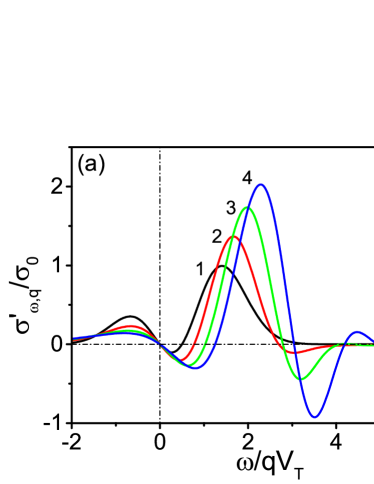
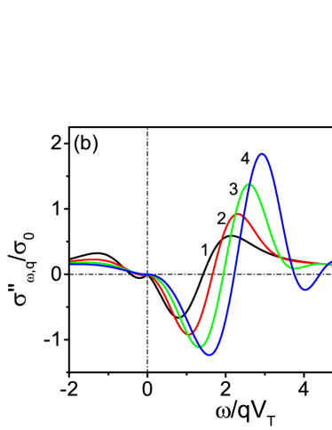
Figure 1: Normalized real (a) and imaginary (b) parts of the dynamic conductivity as functions of the normalized angular frequency at $V_{dr}/V_{T}=0.5$. The vertical dot-dashed line divides each figure into two parts: the right part is for $q>0$, the left one is for $q<0$. Curves $1,\,2,\,3$ and $4$ are for $|\gamma_{q}|=0,\,0.5,\,1$ and $1.5$, respectively.

The conclusions obtained from analytical considerations are supported by the numerical results shown in Figs. 1 and 2. Indeed Figs. 1 (a) and (b) represents the normalized real and imaginary parts of the conductivity, $\sigma_{\omega,q}^{\prime}/\sigma_{0}$ and $\sigma_{\omega,q}^{\prime\prime}/\sigma_{0}$, $\sigma_{0}=2e^{2}n_{0}/m^{*}V_{T}|q|$, as functions of the normalized angular frequency, $\omega/qV_{T}$, for $|\gamma_{q}|=0,\,0.5,\,1$ and $1.5$ at $V_{dr}/V_{T}=0.5$. The right parts of these figures correspond to the case of $q>0,\,\omega>0$, the left parts are for $q<0,\,\omega>0$. The apparent non-reciprocal frequency dispersion of $\sigma_{\omega,q}$ is due to the electrons drift subjected to the stationary field, $E_{0}$. In Figs. 1 (a) and (b), curves labeled by $1$ show normalized $\sigma_{\omega,q}^{\prime}$ and $\sigma_{\omega,q}^{\prime\prime}$ calculated with the use of Eqs. (9) and (10), curves labeled by $2,\,3,\,4$ are calculated according to the result of Eq. (8). These curves demonstrate the importance of the effect of the electric field, $E_{0}$, on the high-frequency electron dynamics. Indeed, at a given $q$ an increase in $\gamma_{q}$ corresponds to a proportional increase of $E_{0}$, this last leading to an oscillatory behavior of both $\sigma_{\omega,q}^{\prime}$ and $\sigma_{\omega,q}^{\prime\prime}$. Moreover, since the real and imaginary parts of $\sigma_{\omega,q}$ are of the same order of magnitude, a large phase shift, $\phi_{\omega}$, between the electric field $\tilde{E}$ and the current $\tilde{j}$ may appear; $\phi_{\omega}$ is strongly dependent on the frequency and can change a sign.

Fig. 1 (a) for $\sigma_{\omega,q}^{\prime}$ shows that an increase of the field, $E_{0}$, produces a widening of the Cerenkov-like region and additional high-frequency regions with $\sigma_{\omega,q}^{\prime}<0$. The oscillatory character of $\sigma_{\omega,q}^{\prime}$ and the above mentioned frequency regions are better evidenced in Fig. 2 where the density plot of $\sigma_{\omega,q}^{\prime}$ is presented as a function of the variables $\{\omega/qV_{T},\,\gamma_{q}\}$, which are dimensionless frequency and dimensionless stationary field for a given $q$. The white regions correspond to $\sigma_{\omega,q}^{\prime}>0$. At $\gamma_{q}<1$, i.e. at weak electric fields, we notice the Cerenkov-like region for small $\omega$ and an additional extensive high-frequency region with $\sigma_{\omega,q}^{\prime}<0$. At $\gamma_{q}>1$, i.e. at large electric fields, there is an alternation of regions with positive and negative $\sigma_{\omega,q}^{\prime}$.

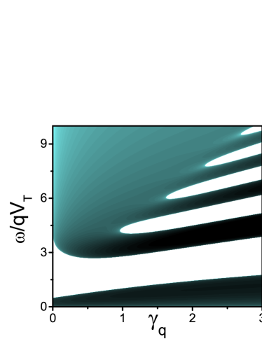
Figure 2: Density plot of the normalized $\sigma_{\omega,q}^{\prime}$ as a function of the dimensionless frequency $\omega/qV_{T}$ and dimensionless electric field $\gamma_{q}$.

The importance of a correct calculation of the high-frequency conductivity with spatial dispersion can be illustrated with a practical example as follows. Consider an AlGaAs/GaAs/AlGaAs quantum well heterostructure covered by a submicron metallic grating. A schematic of such a hybrid plasmonic structure is shown in Fig. 3(a). It is assumed that the structure is doped and there is a 2DEG in the GaAs quantum well layer. A subwavelength metallic grating is placed in the vicinity of the quantum well to provide a strong coupling of electron oscillations and radiation under THz illumination of the plasmonic structure. For the structure we set the following geometrical parameters: $a_{g}=200$ nm, $b_{g}=160$ nm, $d=20$ nm, and $D_{s}=2$ $\mu$m [see Fig. 3(a)]. The sheet electron concentration is assumed to be $n_{0}=3\times 10^{11}$ cm^-2. A stationary lateral electric field, $E_{0}$, applied to the quantum well layer induces a drift of the electrons. Calculations of $T_{e}$ and $V_{dr}$ in the GaAs quantum well can be found elsewhere Kor1 ; Kor2 . The dependencies $T_{e}(E_{0})$ and $V_{dr}(E_{0})$ are presented in Fig. 3(b) for a temperature of $77$ K.

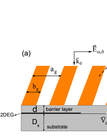
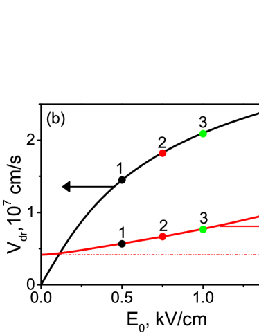
Figure 3: (a): Schematic of the plasmonic structure with 2DEG. (b): Dependencies of the electron temperature and drift velocity on the applied electric field taken from Ref. [Kor2, ]. The dots correspond to the electric fields for which the absorptivity is shown in Fig. 4.

The $V_{dr}(E_{0})$ function can be used to calculate the differential mobility, $\mu_{d}(E_{0})\equiv dV_{dr}/dE_{0}$, and the scattering time, $\tau_{sc}=m^{*}\mu_{d}(E_{0})/e$, of hot electrons. The latter parameter allows us to estimate the criteria necessary for the collisionless approach: $\omega\tau_{sc}\gg 1,ql_{sc}\!=\!q\sqrt{2k_{B}T_{e}/m^{*}}\tau_{sc}\!\!\gg\!\!1$. For example, at $E_{0}=0.5$ kV/cm, we found that $\tau_{sc}=0.65$ ps, $l_{sc}=1.3\times\,10^{-5}$ cm, i.e., for $3...4$ THz frequency range we find that $\omega\,\tau_{sc}\approx 12...16$ and $ql_{sc}\approx 4$ at $q\approx\pi\times 10^{5}$ cm^-1 (characteristic wavevector corresponding to the grating period, $a_{g}$).

Based on the solution of the Maxwell’s equationPopov ; Kor4 and using Eq. (8) together with the above mentioned data on $V_{dr}$ and $T_{e}$, we have calculated the spectral characteristics of the plasmonic structure, including transmittivity, reflectivity and absorptivity. Absorptivity was calculated in usual way as 1 minus a sum of transmittivity and reflectivityTHz-Ampl-2 .

In particular, the spectral dependences of the absorptivity of THz waves calculated for three applied fields $E_{0}=0.5,\,0.75,\,1$ kV/cm (parameters $\gamma_{q}=0.21,0.31,0.39$, respectively) are shown in Fig. 4 by curves 1, 2, 3, respectively. The corresponding values of $T_{e}$ and $V_{dr}$ for these fields are indicated as dots in Fig. 3(b). For comparison, we present also the absorptivity calculated at $T_{e}$ and $V_{dr}$ corresponding to $E_{0}=0.5$ kV/cm, but setting $\gamma_{q}=0$, i.e., neglecting the electric field effect on the electron high-frequency dynamics (dashed line in Fig. 4). The latter calculation put in evidence two peaks of absorption of THz waves related to the excitation of two plasmon waves propagating along the electron drift (higher frequency) and in the opposite direction (lower frequency). In fact, more rigorous calculations for $\gamma_{q}\neq 0$ show that the lower frequency peak of absorption exists, though modified, but at higher frequencies (at $3...4$ THz) the absorptivity becomes negative thus enhancing the intensity of THz radiation at the expense of the stationary field and current. In the corresponding frequency range, the sum of the amplitudes of the refracted and transmitted waves exceeds the incident wave amplitude. For example, at $E_{0}=0.5$ kV/cm and resonant angular frequency $\omega/2\pi=3.18$ THz, the transmittivity and reflectivity are equal to 1.01 and 0.52, respectively. At higher fields, $E_{0}=0.75,\,1$ kV/cm, and corresponding resonant frequencies $\omega/2\pi=3.43,\,3.63$ THz the transmittivity takes the values $0.65$ and $0.59$, respectively, with corresponding reflectivity values of $0.45$ and $0.47$. The negative absorptivity corresponds to additional high-frequency regions with $\sigma_{\omega,q}^{\prime}<0$ (see inset in Fig. 4). The emergence of negative absorptivity corresponds to an energy transfer from the stationary field to the electromagnetic wave interacting with unstable plasmons modes.

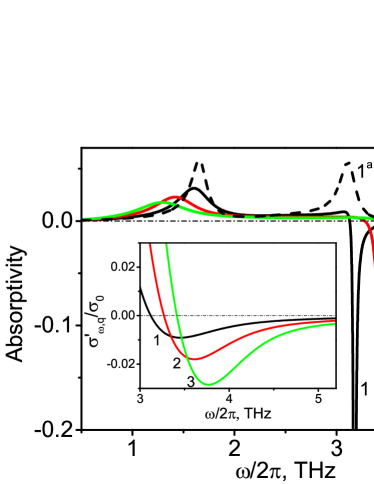
Figure 4: Absorptivity spectra of the plasmonic structure at different applied electric fields indicated in the text. Dashed curve is the absorptivity calculated at $T_{e}$ and $V_{dr}$ corresponding to $E_{0}=0.5$ kV/cm and $\gamma_{q}=0$. Inset: normalized $\sigma_{\omega,q}^{\prime}$ in the frequency range of $3...5$ THz, at $q=\pi\times 10^{5}$ cm^-1 and the same applied electric fields.

The above analysis was conducted for $\sigma_{\omega,q}$ with the use of the shifted Maxwellian distribution, which facilitates the analytical study of $\sigma_{\omega,q}$. Below, we demonstrate how the main features of $\sigma_{\omega,q}$ are reproduced for functions, ${g}_{0}(p_{x})$, obtained by the Monte-Carlo method. We use the results of paperMosko , which were obtained by Monte-Carlo simulations of electron transport in GaAs quantum wells at the parameters similar to already used above. In particular, these results were reported for the ambient temperature $T=60\,K$, $E_{0}=1.2\,kV/cm$ and $n_{0}=2\times 10^{11}$ cm^-2 (i.e., e-e scattering does not completely control electron kinetics). In Fig. 5(a)) we show the shifted Maxwellian distribution (solid line) with parameters $T_{e}=96\,K$ and $V_{dr}=2.48\times 10^{7}\,cm/s$ (parameter $\gamma_{q}=0.47$), and two functions $\bar{g}_{0}(p_{x})$ found Mosko with and without e-e scattering (dashed and dashed-doted lines, respectively). Though all three functions are seemingly quite similar and give the same mean energy and drift velocity, the two latter functions have more sharp decrease at large momenta $p_{x}$. Calculations of $\sigma^{\prime}_{\omega,q}$ for these three functions $\bar{g}_{0}(p_{x})$ are presented in Fig. 5 (b). One can see that all discussed above features of $\sigma^{\prime}_{\omega,q}$ are well reproduced. Noticeable enhancement of the oscillation behavior of $\sigma_{\omega,q}$ found for the functions obtained by the Monte-Carlo method are due to more sharp decrease of the electron stationary distribution at large $p_{x}$.

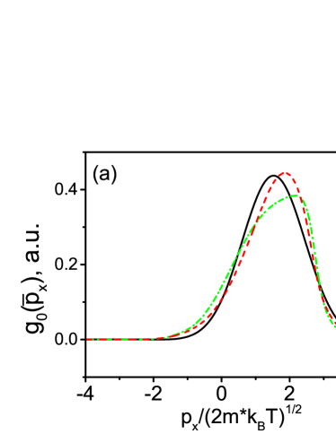
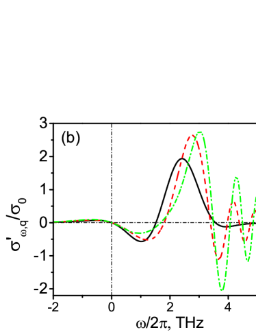
Figure 5: (a): The shifted Maxwellian distribution function $\bar{g}_{0}(p_{x})$ (solid line), distribution functions obtained Mosko by the Monte-Carlo methods with and without e-e scattering (dashed and dashed-dot lines, respectively). (b): function $\sigma^{\prime}_{\omega,q}$ calculated according Eq.(5) for the presented distribution functions. Wavevector $q_{x}$ is the same as in Fig. 4.

Summarizing, we have analyzed the high-frequency conductivity including spatial dispersion for two-dimensional electrons subjected to a high stationary electric field. We have taken into consideration the effects of the stationary electric field on both the stationary electron distribution and the high-frequency dynamics of the electrons. In the collisionless approximation we have found that the high-frequency conductivity with spatial dispersion exhibits the following features contrasting to the case of dissipative transport: strong non-reciprocal effect, oscillatory behavior and a set of frequency region with negative values of the real part of the conductivity. If the 2DEG plasmon frequency is in one of these regions, the current-driven 2DEG is unstable, i.e. the plasma oscillations will grow in time and along the electron drift (so-called convective instability). Under these conditions, an incident THz wave can be amplified in a properly designed hybrid plasmonic structure. Similarly, in a hybrid system composed of electrostatically coupled quantum well and a polarizable nanoparticle (a quantum dot, a molecule, etc.), the electron drift in the stationary electric field will provide excitation and instability of this hybrid system if the dipole oscillation frequency of the nanoparticle is in one of the discussed frequency regionsKukhtaruk1 .

We suggest that the discovered features associated with the electron response to high-frequency and spatially nonuniform electromagnetic fields are of general character. The obtained results can be used for the refining of near-field THz microscope techniques and the development of THz devices with a lateral nanostructuring.

This work is supported by the German Federal Ministry of Education and Research (BMBF Project 01DK17028).

References

- (1) Ho-Jin Song, Tadao Nagatsuma, Handbook of Terahertz Technologies: Devices and Applications, CRC Press, 2015.
- (2) M. Dyakonov and M. Shur, Phys. Rev. Lett. 71, 2465 (1993).
- (3) S.A. Mikhailov, Recent Res. Devel. Applied Phys. 2, 65 (1999); Phys. Rev. B58, 1517 (1998).
- (4) S. A. Mikhailov, N. A. Savostianova and A. S. Moskalenko, Phys. Rev. B 94, 035439 (2016).
- (5) P. Bakshi, K. Kempa, A. Scorupsky, C. G. Du, and G. Feng, R. Zobl, G. Strasser, C. Rauch, Ch. Pacher, K. Unterrainer, and E. Gornik., Appl. Phys. Lett., 75, 1685 (1999).
- (6) T. Otsuji, Y. M. Meziani, M. Hanabe, T. Nishimura, E. Sano, Solid-State Electronics 51, 1319 (2007).
- (7) T. Otsuji, H. Karasawa, T. Watanabe, T. Suemitsu, M. Suemitsu, E. Sano, W. Knap and V. Ryzhii, C. R. Physique 11, 421-432 (2010).
- (8) R. Hillenbrandt, T. Taubner and F. Keilmann, Nature 418, 159 (2002).
- (9) R. Hillenbrand and F. Keilmann, Appl. Phys. Lett. 80, 25 (2002).
- (10) H.F.Hamann. M. Larbadi, S.Barzen, T.Brown, A.Gallagher, J. Nesbitt, Optics Communications, 227, 1-13 (2003).
- (11) The phase-mixing property of an equation means that any solution converges weakly at large time to a spatially homogeneous distribution. The mathematical proof of this property for the BTE is analyzed in C. Mouhot, C. Villani, Acta Math., 207 , 29 (2011).
- (12) L. D. Landau, Zhurnal Eksper. Teoret. Fiz. 16, 574 (1946) [Acad. Sci. USSR. J. Phys. 10, 25 (1946)].
- (13) E. M. Lifshitz and L. P. Pitaevski, Course of Theoretical Physics Physical Kinetics, Vol. 10, Pergamon Press, Oxford-New York, 1981.
- (14) N. M. Temme, Error Functions, Dawson’s and Fresnel Integrals, in F.W.J Olver, D. M. Lozier, R.F. Boisvert, Ch. W.Clark, NIST Handbook of Mathematical Functions, Cambridge University Press, 2010.
- (15) D. K. Ferry, Semiconductors, Macmillan, New York, 1991.
- (16) M. Moko and A. Mokov, Phys. Rev. B 44(19), 10794 (1991).
- (17) V.V. Korotyeyev, G.I. Syngayivska, V.A. Kochelap and A.A. Klimov, Semiconductor Physics, Quantum Electronics & Optoelectronics 12(4), 328 (2009).
- (18) S. M. Komirenko, K. W. Kim, V. A. Kochelap, V. V. Koroteev and M. A. Stroscio, Phys. Rev B 68, 155308 (2003).
- (19) V.V. Korotyeyev, Semiconductor Physics, Quantum Electronics & Optoelectronics, 18(1), 1 (2015).
- (20) Eq. (9) coincides with the response function calculated by the Landau method Landau using the shifted Maxwellian distribution (6).
- (21) G. Ecker, Theory of fully ionized plasmas, Academic Press, New York and London , 1972.
- (22) O.R. Matov, O.V. Polischuk and V.V. Popov, Int. J. Infrared Millimeter Waves 14 (7), 1455 (1993).
- (23) Yu. M. Lyaschuk and V.V. Korotyeyev, Ukr. J. Phys. 62(10), 889 (2017).
- (24) V. A. Kochelap and S. M. Kukhtaruk, J. Appl. Phys., 109, 114318 (2011).