Multiresolution time-of-arrival estimation from multiband radio channel measurements

Abstract

Achieving high resolution time-of-arrival (TOA) estimation in multipath propagation scenarios from bandlimited observations of communication signals is challenging because the multipath channel impulse response (CIR) is not bandlimited. Modeling the CIR as a sparse sequence of Diracs, TOA estimation becomes a problem of parametric spectral inference from observed bandlimited signals. To increase resolution without arriving at unrealistic sampling rates, we consider multiband sampling approach, and propose a practical multibranch receiver for the acquisition. The resulting data model exhibits multiple shift invariance structures, and we propose a corresponding multiresolution TOA estimation algorithm based on the ESPRIT algorithm. The performance of the algorithm is compared against the derived Cramér Rao Lower Bound, using simulations with standardized ultra-wideband (UWB) channel models. We show that the proposed approach provides high resolution estimates while reducing spectral occupancy and sampling costs compared to traditional UWB approaches.

Index Terms—  time-of-arrival, multiresolution estimation, cognitive radio, multiband sampling, multipath channel estimation

1 Introduction

Time-of-arrival (TOA) estimation usually starts with the estimation of the underlying multipath communication channel. As the channel frequency response (CFR) is not bandlimited while we can only probe the channel with bandlimited signals, modeling assumptions are required. Traditionally, the channel impulse response (CIR) is modeled as an FIR filter of limited time duration, and the resulting time resolution for TOA estimation is inversely proportional to the sampling rate, i.e., to the bandwidth of the probing signal. This motivates the use of ultra-wideband (UWB) systems [1, 2], but at the cost of large spectrum occupancy, high sampling, and high computational requirements at the receiver.

High resolution techniques therefore refine the channel model by considering a parametric model consisting of a small number of attenuated and delayed Diracs. Under this assumption, theoretically we only need to take an equally small number of samples in the frequency domain. The main challenge is to devise practical and robust schemes for implementing this.

In the past, many delay estimation algorithms have been proposed, and they can be classified into methods based on (i) subspace estimation [3, 4, 5], (ii) finite rate of innovation [6, 7, 8], and (iii) compressed sampling signal reconstruction [9, 10, 11, 12, 13, 14]. Some of these methods are not quite robust to noise, while other methods require a separate receiver chain for each multipath component, which may not be practical.

To improve resolution, a large frequency band (aperture) must be covered, while to limit sampling rates, the total band should not be densely sampled. This motivates the use of multiband acquisition systems, for e.g., [15] proposes estimation from a set of “dispersed” Fourier coefficients. Other methods include for e.g., bandpass sampling, multicoset sampling and modulated wideband converter (MWC) [16], where the implementation at the analog front-end is not straight forward.

In this paper, we aim at a limited complexity high resolution TOA estimation algorithm and consider coherent multiband acquisition. In a multichannel receiver, each receiver chain will coherently sample one of the sub-bands, which can be implemented with off-the-shelf radio frequency (RF) components. By stacking the observations into Hankel matrices, the resulting data model has precisely the form of Multiple Invariance ESPRIT [17], so that the related algorithms are applicable, in particular, the Multiresolution ESPRIT algorithm [18], which was aimed at carrier frequency estimation.

Similar to [18], we propose an algorithm where the invariance structure of a single sub-band will provide coarse parameter estimates, while the the invariance structure of the lowest against the highest frequency sub-band will provide high-resolution, but phase wrapped, estimates. The wrapping is resolved using the coarse estimates.

The resulting algorithm is benchmarked through simulations, by comparing its performance with the Cramér Rao Lower Bound (CRLB). The results show that the proposed approach provides high resolution estimates while reducing spectral occupancy and sampling costs compared to classical UWB approaches, paving the way for cognitive radio ranging systems.

2 Problem Formulation and Data Model

Channel model: We consider a channel model which is appropriate for modeling the multipath propagation of wideband and UWB signals. The multipath channel with $K$ propagation paths is defined by a continuous-time impulse response $\widetilde{h}(t)$ and its continuous time frequency transform (CTFT) $\widetilde{H}(\Omega)$ as

$$\widetilde{h}(t)=\sum_{k=1}^{K}\widetilde{\alpha}_{k}\delta(t-\tau_{k})\quad\text{and}\quad\widetilde{H}(\Omega)=\sum_{k=1}^{K}\widetilde{\alpha}_{k}e^{-j\Omega\tau_{k}},$$ (1)

where we use “tilde” to represent signals at RF frequencies, $\widetilde{\alpha}_{k}\in\mathbb{R}$ and $\tau_{k}\in\mathbb{R}_{+}$ represent the gain and time-delay of the $k$th resolvable path [19]. This model neglects the effects of frequency dependent distortions [20]. However, for the purpose of our analysis, it provides sufficient characterization of the radio signal propagation.

Continuous-time signal model: The objective in the paper is to estimate the $2K$ channel parameters by probing the channel by a wideband training signal $\widetilde{s}(t)$. Assume that $\widetilde{s}(t)$ covers (at least) $L$ separate bands $\mathcal{W}_{i}=[\Omega_{i}-\frac{1}{2}B_{i},\Omega_{i}+\frac{1}{2}B_{i}]$, $i=1,\cdots,L$, where $\Omega_{i}$ is the center frequency and $B_{i}$ is the bandwidth of the $i$th sub-band. The CTFT of $\widetilde{s}(t)$ is

$$\widetilde{S}(\Omega)=\begin{cases}\widetilde{S}_{i}(\Omega),&\Omega\in\mathcal{W}_{i},\;i=1,\cdots,L\\ \mbox{arbitrary},&\text{otherwise}\,.\end{cases}$$ (2)

The received signal is $\widetilde{x}(t)=\widetilde{s}(t)\ast\widetilde{h}(t)+\widetilde{n}(t)$, where $\widetilde{n}(t)$ represents additive white Gaussian noise. The corresponding CTFT is (cf. Fig. 1a)

$$\widetilde{X}(\Omega)=\widetilde{H}(\Omega)\widetilde{S}(\Omega)+\widetilde{N}(\Omega)\,.$$ (3)

Now, consider a multibranch receiver having $L$ RF chains and complex sampling ADCs as shown in Fig. 1b. The $i$th RF chain bandlimits $\widetilde{X}(\Omega)$ to $\Omega\in\mathcal{W}_{i}$, and performs complex downconversion to baseband, possibly followed by additional lowpass filtering before sampling at Nyquist. We model this by an equivalent lowpass filter $G_{i}(\Omega)$ with passband $\mathcal{B}_{i}=[-\frac{1}{2}B_{i},\frac{1}{2}B_{i}]$. The CTFT of the signal $x_{i}(t)\in\mathbb{C}$ received in the $i$th branch at baseband is thus given by

$$X_{i}(\Omega)=\begin{cases}G_{i}(\Omega)H_{i}(\Omega)S_{i}(\Omega)+N_{i}(\Omega),&\Omega\in\mathcal{B}_{i}\\ 0,&\text{otherwise}\end{cases}$$ (4)

where $N_{i}(\Omega)$ is bandlimited white Gaussian noise and $\{H_{i}(\Omega)$, $S_{i}(\Omega),G_{i}(\Omega)\}$ are the complex baseband equivalents of $\{\widetilde{H}(\Omega)$, $\widetilde{S}(\Omega),\widetilde{G}(\Omega)\}$. In particular, $H_{i}(\Omega)=\widetilde{H}(\Omega+\Omega_{i})$.

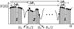
(a)

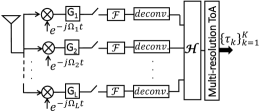
(b)

Fig. 1: (a) The multiband channel frequency response, and (b) a multibranch receiver with $L$ RF chains.

Discrete-time data model: Assume for theoretical purposes, that $x_{i}(t)$ has a finite duration $T$, and is zero (or periodic) outside this interval. For simplicity of exposition, we will consider that the bandwidths of the signals and the sampling periods in all receiver branches are the same, that is $B_{i}=B$ and $T_{s,i}=T_{s}$ for all $i\in[1,L]$. We sample $x_{i}(t)$ with period $T_{s}$, and take $N$ samples on the nonzero interval such that $T=NT_{s}$. Let $\Omega_{s}=2\pi/T_{s}$, then the $N$-point DFT of $x_{i}(t)$ is given by

$$X_{i}[n]=G_{i}[n]H_{i}[n]S_{i}[n]+N_{i}[n],\quad n=0,\cdots,N-1$$ (5)

with, in particular,

$$H_{i}[n]=H_{i}\left(\frac{n}{N}\Omega_{s}\right)=\widetilde{H}(\frac{n}{N}\Omega_{s}+\Omega_{i})\,.$$

Inserting the channel model (1) gives

$$H_{i}[n]=\sum_{k=1}^{K}\widetilde{\alpha}_{k}e^{-j\Omega_{i}\tau_{k}}e^{-jn\Omega_{t}\tau_{k}}$$ (6)

where $\Omega_{t}=\frac{1}{N}\Omega_{s}=\frac{2\pi}{T}$.

Let us stack the $N$ samples of $X_{i}[n]$ into a vector $\bm{x}_{i}$, and likewise for $\bm{g}_{i}$, $\bm{h}_{i}$, $\bm{s}_{i}$, and $\bm{n}_{i}$. The data model (5) then becomes

$$\bm{x}_{i}=\bm{h}_{i}\odot\bm{g}_{i}\odot\bm{s}_{i}+\bm{n}_{i}\,.$$ (7)

where $\odot$ denotes a pointwise multiplication. The channel model (6) can be written as

$$\bm{h}_{i}=\bm{M}\bm{\Theta}_{i}\bm{\alpha}\,,$$ (8)

where $\bm{M}$ is the $N\times K$ Vandermonde matrix

$$\bm{M}=\begin{bmatrix}1&1&\cdots&1\\ \Phi_{1}&\Phi_{2}&\cdots&\Phi_{K}\\ \vdots&\vdots&\ddots&\vdots\\ \Phi_{1}^{{N-1}}&\Phi_{2}^{N-1}&\cdots&\Phi_{K}^{N-1}\end{bmatrix}\,,\quad$$ (9)

and $\Phi_{k}=e^{-j\phi_{k}}$, where $\phi_{k}=\Omega_{t}\tau_{k}$. Likewise,

$$\bm{\Theta}_{i}=\begin{bmatrix}\Theta_{i,1}&&\bm{0}\\ &\ddots&\\ \bm{0}&&\Theta_{i,K}\end{bmatrix}\,,\qquad\bm{\alpha}=\begin{bmatrix}\widetilde{\alpha}_{1}\\ \vdots\\ \widetilde{\alpha}_{K}\end{bmatrix}$$ (10)

and $\Theta_{i,k}=e^{-j\theta_{i,k}}$, where $\theta_{i,k}=\Omega_{i}\tau_{k}$.

Next, we apply deconvolution to the data vector (7). Assume that no entry of $\bm{g}_{i}$ and $\bm{s}_{i}$ is zero or close to zero. As the entries of these vectors are known from training and filter design/calibration, the deconvolution step to estimate the DFT channel coefficients is written as

$$\bm{h}_{i}=\{\text{diag}(\bm{g}_{i}\odot\bm{s}_{i})\}^{-1}\bm{x}_{i},$$ (11)

which satisfies the model

$$\bm{h}_{i}=\bm{M}\bm{\Theta}_{i}\alpha+\bm{n}^{\prime}_{i},$$ (12)

where $\bm{n}^{\prime}_{i}$ is a zero mean circular symmetric complex Gaussian distributed noise vector. It is common that the power spectral densities of the signal or the filters are not perfectly flat. In that case, the noise vector is not white, but the coloring is known and can be taken into account.

3 Multiresolution Delay Estimation

Our next objective is to estimate the $K$ time-delays $\{{\tau_{k}}\}_{k=1}^{K}$. We begin with an algorithm for estimating these time-delays using a single frequency band, and later extend it for the multiple bands. The single band algorithm is in fact classical (cf. [3, 21, 22] and earlier references).

3.1 Single band estimation algorithm

From a single vector $\bm{h}_{i}$, we construct a Hankel matrix of size $P\times Q$ as

$$\bm{\mathcal{H}}_{i}=\begin{bmatrix}H_{i}[0]&H_{i}[1]&\cdots&H_{i}[Q]\\ H_{i}[1]&H_{i}[2]&\cdots&H_{i}[Q+1]\\ \vdots&\vdots&\ddots&\vdots\\ H_{i}[P-1]&H_{i}[P]&\cdots&H_{i}[N-1]\end{bmatrix}\,.$$ (13)

Here, $P=N-Q-1$, and we require $P>K$ and $Q\geq K$. From (12), and using the shift invariance of the Vandermonde matrix (9), the Hankel matrix satisfies

$$\bm{\mathcal{H}}_{i}=\bm{M}^{\prime}\bm{\Theta}_{i}\bm{A}+\bm{N}_{i}\,,$$ (14)

where $\bm{M}^{\prime}$ is an $P\times K$ submatrix of $\bm{M}$, and $\bm{N}_{i}$ is a noise matrix. Furthermore,

$$\bm{A}=[\bm{\alpha},\,\bm{\Phi}\bm{\alpha},\,\bm{\Phi}^{2}\bm{\alpha},\cdots,\bm{\Phi}^{Q-1}\bm{\alpha}]\,$$

where $\mathbf{\Phi}=\text{diag}([\phi_{1}\cdots\phi_{K}])$.

Since (14) resembles the data model of the classical ESPRIT algorithm, $\bm{\Phi}$ can be estimated by exploiting the low-rank approximation of the Hankel matrix and its shift-invariance properties. From $\bm{\Phi}$, the parameters $\tau_{k}$ immediately follow.

In particular, let $\bm{U}$ be a $K$-dimensional orthonormal basis for the column span of $\bm{\mathcal{H}}_{i}$, obtained using the singular value decomposition, then we can write $\bm{M}^{\prime}=\bm{U}\bm{T}$, where $\bm{T}$ is a $K\times K$ nonsingular matrix. Next, let us define selection matrices

$$\bm{J}_{1}^{(1)}=[\bm{I}_{P-r}\quad\bm{0}_{P-r,r}],\qquad\bm{J}_{2}^{(1)}=[\bm{0}_{P-r,r}\quad\bm{I}_{P-r}],$$ (15)

where $\bm{I}_{P-r}$ is identity matrix of size $(P-r)\times(P-r)$ and $\mathbf{0}_{P-r,r}$ is a zero matrix of size $(P-r)\times r$. For $r=1$, $\bm{U}_{1}=\bm{J}_{1}^{(1)}\bm{U}$ and $\bm{U}_{2}=\bm{J}_{2}^{(1)}\bm{U}$ are submatrices of $\bm{U}$ obtained by dropping its first and, respectively, last row. In view of the shift invariance structure of $\bm{M}^{\prime}$, we have

$$\bm{U}_{1}=\bm{M}_{1}^{\prime}\bm{T}^{-1}\,,\qquad\bm{U}_{2}=\bm{M}_{1}^{\prime}\bm{\Phi}\bm{T}^{-1}$$ (16)

where $\bm{M}_{1}^{\prime}=\bm{J}_{1}^{(1)}\bm{M}^{\prime}$. Finally, we form the matrix $\bm{\Psi}=\bm{U}_{1}^{\dagger}\bm{U}_{2}$ where $\dagger$ denotes pseudo-inverse. $\bm{\Phi}$ can then be estimated directly from the eigenvalue decomposition of $\bm{\Psi}$, as it satisfies the model

$$\bm{\Psi}=\bm{T}\bm{\Phi}\bm{T}^{-1}\,.$$ (17)

In other words, let $\hat{\lambda}_{k}$ be an estimate of the $k$th eigenvalue of $\bm{\Psi}$, then the corresponding time delay estimate is ${\tau}_{k}=\text{arg}\{\lambda_{k}\}/\Omega_{t}$. Since $\Omega_{t}\tau_{k}<2\pi$ because $\tau_{k}<T$, there is no phase wrapping issue here. Note that for TOA estimation, we are mostly interested in retrieving the smallest $\tau_{k}$ as it belongs to the line-of-sight propagation, i.e., true distance.

3.2 Multiresolution estimation algorithm

The aforementioned algorithm used data from a single sub-band and has a limited resolution, since it is based on the shift of one row in the Hankel matrix $\bm{\mathcal{H}}_{i}$, which results in only a small phase shift $\Omega_{t}\tau_{k}$. Note that the sampling rate does not play a role in $\Omega_{t}$, only the total signal duration $T$. Thus, oversampling would increase the signal-to-noise ratio (SNR) but not the resolution.

The matrix $\bm{M}$ is also invariant for shifts over multiple rows, and therefore, if $N$ is sufficiently large, then we can increase the resolution by considering shifts of multiple rows of $\bm{\mathcal{H}}_{i}$. Indeed, a shift of $r$ rows using shift matrices $\bm{J}_{1}^{(r)},\bm{J}_{2}^{(r)}$ (or by interleaving rows of $\bm{\mathcal{H}}_{i}$ [8]) leads to an estimate of $\bm{\Phi}^{r}$. Unfortunately, phase shifts have an ambiguity of multiples of $2\pi$, so that approaches for increasing the resolution introduce ambiguity in the estimates for the $\tau_{k}$. If $T$ is not very large, this approach is limited.

Here, we are interested in an algorithm for high resolution and unambiguous estimation of the $\tau_{k}$ from multiband channel estimates $\bm{h}_{i}$, where $i=1,\cdots,L$. For simplicity of exposition, we will consider for the moment only two bands (i.e., $i=1,2$), with central frequencies $\Omega_{1}$ and $\Omega_{2}$. Following the procedure described in Section 3.1, we form the Hankel matrices $\bm{\mathcal{H}}_{i}$ defined in (13) and stack them in a matrix

$$\bm{\mathcal{H}}=\begin{bmatrix}\bm{\mathcal{H}}_{1}\\ \bm{\mathcal{H}}_{2}\end{bmatrix}.$$

The matrix $\bm{\mathcal{H}}$ has the model

$$\bm{\mathcal{H}}=\begin{bmatrix}\bm{M}^{\prime}\\ \bm{M}^{\prime}\bm{\Theta}\end{bmatrix}\bm{\Theta}_{1}\bm{A}+\bm{N}\,,$$ (18)

where $\bm{\Theta}=\bm{\Theta}_{2}\bm{\Theta}_{1}^{-1}$, $\bm{\Theta}_{1}$ and $\bm{\Theta}_{2}$ are given in (10), and $\bm{N}$ is formed by stacking $\bm{N}_{1}$ on top of $\bm{N}_{2}$. Note that $\bm{\mathcal{H}}$ has a double shift invariance structure introduced by the phase shifts of the $\tau_{k}$ on the (i) sampling frequency within a single band, $\phi_{k}$, and (ii) carrier frequency difference between two bands, $\theta_{k}=\theta_{2,k}-\theta_{1,k}$, as shown in Fig.  1a [23]. In general, the carrier frequency difference is much higher than the sampling frequency, and therefore, $\theta_{k}\gg\phi_{k}$ for $k=1,\cdots,K$. The estimation of the $\tau_{k}$ from $\bm{\Theta}$ will result in high resolution but ambiguous estimates, due to unknown multiples of $2\pi$ in the phases. However, we can use the idea of multiresolution parameter estimation [18] to develop the algorithm for high resolution estimation of the $\tau_{k}$ without ambiguity by combining coarse and fine estimates obtained from $\bm{\Phi}$ and $\bm{\Theta}$, respectively.

We follow a similar approach as in the previous section. Let $\bm{U}$ be an orthonormal basis for the column span of $\bm{\mathcal{H}}$, obtained using a truncated SVD. Define the selection matrices

$$\centering\bm{J}_{\Phi 1}^{(r)}=\bm{I}_{2}\otimes[\bm{I}_{P-r}\quad\bm{0}_{P-r,r}], \qquad\bm{J}_{\Theta 1}=[1\quad 0]\otimes\bm{I}_{P},$$ (19)

$$\bm{J}_{\Phi 2}^{(r)}=\bm{I}_{2}\otimes[\bm{0}_{P-r,r}\quad\bm{I}_{P-r}], \qquad\bm{J}_{\Theta 2}=[0\quad 1]\otimes\bm{I}_{P}.$$

To estimate $\bm{\Phi}$, we set $r=1$ and take submatrices consisting of the first and, respectively, the last row of each block matrix stacked in $\bm{U}$, that is $\bm{U}_{\Phi 1}=\bm{J}_{\Phi 1}^{(1)}\bm{U}$ and $\bm{U}_{\Phi 2}=\bm{J}_{\Phi 2}^{(1)}\bm{U}$. The estimation of $\bm{\Theta}$ is based on the first and, respectively, second block matrix present in $\bm{U}$, that is $\bm{U}_{\Theta 1}=\bm{J}_{\Theta 1}\bm{U}$ and $\bm{U}_{\Theta 2}=\bm{J}_{\Theta 2}\bm{U}$. The selected matrices have the following models:

$$\bm{U}_{\Phi 1} =\begin{bmatrix}\bm{M}^{\prime\prime}\\ \bm{M}^{\prime\prime}\bm{\Theta}\end{bmatrix}\bm{\Theta}_{1}\bm{T}^{-1}, \qquad\bm{U}_{\Theta 1} =\bm{M}^{\prime}\bm{T}^{-1},$$ (20)

$$\bm{U}_{\Phi 2} =\begin{bmatrix}\bm{M}^{\prime\prime}\\ \bm{M}^{\prime\prime}\bm{\Theta}\end{bmatrix}\bm{\Phi}\bm{\Theta}_{1}\bm{T}^{-1}, \qquad\bm{U}_{\Theta 2} =\bm{M}^{\prime}\bm{\Theta}\bm{T}^{-1},$$

where $\bm{M}^{\prime\prime}=\bm{J}_{1}^{(1)}\bm{M}^{\prime}$ and $\bm{J}_{1}^{(1)}$ is given in (15). The Least Squares approximate solutions to the set of equations in (20) satisfy a model of the form

$$\bm{\Psi} :=\bm{U}_{\Phi 1}^{\dagger}\bm{U}_{\Phi 2}=\bm{T}\bm{\Phi}\bm{T}^{-1},$$ (21)

$$\bm{\Upsilon} :=\bm{U}_{\Theta 1}^{\dagger}\bm{U}_{\Theta 2}=\bm{T}\bm{\Theta}\bm{T}^{-1}.$$

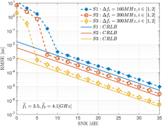
(a)

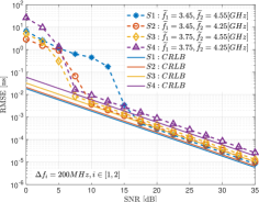
(b)

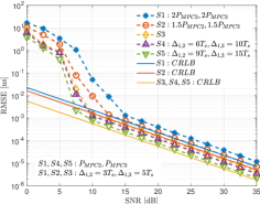
(c)

Fig. 2: Root Mean Square Error (RMSE) of TOA estimates (${\tau}_{1}$) for: (a) varying bandwidths, (b) varying band positions and (c) varying power and spacing of second and third MPC.

Observe that $\bm{\Psi}$ and $\bm{\Upsilon}$ are jointly diagonalizable by the same matrix $\bm{T}$. If each submatrix in (20) has at least $K$ rows, the joint diagonalization can be computed by means of QZ iterations or Jacobi iterations [24, 25, 26]. After $\bm{T}$ has been determined, the parameters $\phi_{k}$ and $\theta_{k}$ for $k=1,\cdots,K$ are estimated.

Based on the phase estimates, coarse and fine time-delays of the delays are computed as

$$\tau_{k}=\Omega_{t}^{-1}\phi_{k}=(\Omega_{2}-\Omega_{1})^{-1}(\theta_{k}+2\pi n_{k}).$$ (22)

The unknown number of cycles $n_{k}$ is determined as the best fitting integer that satisfies (22), that is,

$$n_{k}=\text{round}\left\{\frac{1}{2\pi}\left(\Omega_{t}^{-1}(\Omega_{2}-\Omega_{1})\phi_{k}-\theta_{k}\right)\right\}.$$ (23)

If the estimation errors of the $\phi_{k}$ and the $\theta_{k}$ are comparable, then the $\tau_{k}$ estimate based on $\theta_{k}$ is $\Omega_{t}^{-1}(\Omega_{2}-\Omega_{1})$ times more accurate and less affected by noise compared to the one based on $\phi_{k}$. Therefore, the final estimate of $\phi_{k}$ is obtained based on $\theta_{k}$, or by optimal combining of coarse and fine estimates [18].

This technique can be extended to $L$ matrices. Alternatively, we only consider pairwise estimates, gradually increasing the resolution until we are able to reliably estimate the amount of $2\pi$ phase wraps for the largest shift ($\Omega_{L}-\Omega_{1}$).

4 Results

4.1 Cramér Rao Lower Bound (CRLB)

We use the CRLB as a benchmark to study the performance of the algorithm derived in Section 3.2. The model (12) can be written as

$$\mathbf{h}_{i}=\mathbf{B}_{i}\bm{\alpha}+\mathbf{n}_{i},$$ (24)

where $\mathbf{B}_{i}=\mathbf{M}\bm{\Theta}_{i}=[\mathbf{m}_{1}\Theta_{i,1},\;\mathbf{m}_{2}\Theta_{i,2},\;\dots\;\mathbf{m}_{K}\Theta_{i,K}]$, $\mathbf{m}_{k}$ for $k=1,\cdots,K$ are the columns of $\mathbf{M}$ and $\mathbf{n}_{i}\sim\mathcal{C}\mathcal{N}(\mathbf{0},\sigma^{2}\mathbf{I}_{N})$. The $\mathbf{B}_{i}$ is parameterized by $\bm{\tau}=[\tau_{1},\cdots,\tau_{K}]^{T}$. Under the assumption that the unknown multipath parameters $\bm{\alpha}$ and $\bm{\tau}$ are deterministic, the CRLB for estimating of $\bm{\tau}$, conditioned on complex path attenuations $\bm{\alpha}$, is given by [27]

$$\text{CRLB}(\bm{\tau})=\dfrac{\sigma^{2}}{2}\left\{\Re\left[\mathbf{D}^{H}\mathbf{P}_{\mathbf{B}_{i}}^{\perp}\mathbf{D}\odot\mathbf{R}_{\bm{\alpha}}\right]^{-1}\right\},$$ (25)

where $\mathbf{D}=\left[\dfrac{\partial\mathbf{b}_{i}(\tau_{1})}{\partial\tau_{1}},\dots,\dfrac{\partial\mathbf{b}_{i}(\tau_{K})}{\partial\tau_{K}}\right]$, $\mathbf{b}_{i}(\tau_{k})=\mathbf{m}_{k}\theta_{i,k}$ is the $k$th column of $\mathbf{B}_{i}$, $\mathbf{P}_{\mathbf{B}_{i}}^{\perp}=\mathbf{I}_{N}-\mathbf{B}_{i}(\mathbf{B}_{i}^{H}\mathbf{B}_{i})^{-1}\mathbf{B}_{i}$ and $\mathbf{R}_{\bm{\alpha}}=E\{\bm{\alpha}\bm{\alpha}^{H}\}$. It is straightforward to extend the CRLB for the multiband case by creating the overall data model in the form (24).

4.2 Simulations

We consider a standard outdoor UWB channel model to evaluate the performance of the proposed algorithm [28]. The channel (1) has eight dominant multipath components (MPCs). The first MPC has $8$ times higher power in comparison to the second MPC. The continuous time is modeled using a $3$ GHz grid, where the channel tap delays are spaced at $333.33$ ps. In the simulations, we assume that the TOA is estimated using two bands with central frequencies at $\widetilde{f}_{i}=\Omega_{i}/(2\pi)$ and bandwidths $\Delta f_{i}=B_{i}/(2\pi)$ for $i\in[1,2]$. We use Root Mean Square Error (RMSE) as a metric for evaluation, which is obtained over $10^{4}$ independent Monte Carlo runs. These results are compared against the numerically computed CRLB (25).

In Fig. 2a, the RMSEs of the estimated TOAs (${\tau}_{1}$) for the first MPC are plotted against SNR for the frequency bands with bandwidths $[160,200,300]$ MHz. The proposed algorithm asymptotically achieves the CRLB, for increasing SNR. As expected, for larger bandwidths the proposed algorithm is more robust to noise, and offers higher resolution.

In Fig. 2b, the RMSEs of ${\tau}_{1}$ are plotted against SNR, for various positions of the $200$ MHz wide bands. It can be seen that by increasing the distance between two bands, i.e. frequency aperture, the resolution of the ${\tau}_{1}$ increases for high SNR. However, for low SNR the proposed algorithm has better performance in scenarios where the frequency aperture is lower which is a consequence of lower error for fine time-delay estimation.

Fig. 2c shows the RMSEs of the ${\tau}_{1}$ with respect to SNR for the following scenarios. Firstly, in scenarios S1 and S2, we consider the power of the second ($P_{MPC2}$) and third ($P_{MPC3}$) multipath components increased 2 or 1.5 times as compared to their value in S3, respectively. In scenarios S4 and S5 the distance between main and second ($\Delta_{1,2}$) and third ($\Delta_{1,3}$) MPC has been increased 2 or 3 times as compared to S3, respectively. As expected, the proposed algorithm is less robust to noise and has a lower resolution for scenarios where close MPCs have high power. It is seen, that the resolution of ${\tau}_{1}$ increases in scenarios where the main MPCs are more separated.

References

- [1] S. Gezici et al., “Localization via ultra-wideband radios: a look at positioning aspects for future sensor networks,” IEEE signal processing magazine, vol. 22, no. 4, pp. 70–84, 2005.
- [2] K. Witrisal et al., “Noncoherent ultra-wideband systems,” IEEE Signal Processing Magazine, vol. 26, no. 4, 2009.
- [3] A.-J. Van der Veen, M. C. Vanderveen, and A. Paulraj, “Joint angle and delay estimation using shift-invariance techniques,” IEEE Transactions on Signal Processing, vol. 46, no. 2, pp. 405–418, 1998.
- [4] X. Li and K. Pahlavan, “Super-resolution TOA estimation with diversity for indoor geolocation,” IEEE Transactions on Wireless Communications, vol. 3, no. 1, pp. 224–234, 2004.
- [5] M. Pourkhaatoun and S. A. Zekavat, “High-resolution low-complexity cognitive-radio-based multiband range estimation: Concatenated spectrum vs. Fusion-based,” IEEE Systems Journal, vol. 8, no. 1, pp. 83–92, 2014.
- [6] I. Maravic, J. Kusuma, and M. Vetterli, “Low-sampling rate UWB channel characterization and synchronization,” Journal of Communications and Networks, vol. 5, no. 4, pp. 319–327, Dec 2003.
- [7] M. Vetterli, P. Marziliano, and T. Blu, “Sampling signals with finite rate of innovation,” IEEE transactions on Signal Processing, vol. 50, no. 6, pp. 1417–1428, 2002.
- [8] I. Maravic and M. Vetterli, “Sampling and reconstruction of signals with finite rate of innovation in the presence of noise,” IEEE Transactions on Signal Processing, vol. 53, no. 8, pp. 2788–2805, 2005.
- [9] K. M. Cohen et al., “Channel estimation in UWB channels using compressed sensing,” in Acoustics, Speech and Signal Processing (ICASSP), 2014 IEEE International Conference on. IEEE, 2014, pp. 1966–1970.
- [10] M. Mishali and Y. C. Eldar, “Blind multiband signal reconstruction: Compressed sensing for analog signals,” IEEE Transactions on signal processing, vol. 57, no. 3, pp. 993–1009, 2009.
- [11] M. Mishali, Y. C. Eldar, and A. J. Elron, “Xampling: Signal acquisition and processing in union of subspaces,” IEEE Transactions on Signal Processing, vol. 59, no. 10, pp. 4719–4734, 2011.
- [12] P. Zhang et al., “A compressed sensing based ultra-wideband communication system,” in Communications, 2009. ICC’09. IEEE International Conference on. IEEE, 2009, pp. 1–5.
- [13] K. Gedalyahu and Y. C. Eldar, “Time-delay estimation from low-rate samples: A union of subspaces approach,” IEEE Transactions on Signal Processing, vol. 58, no. 6, pp. 3017–3031, 2010.
- [14] K. Gedalyahu, R. Tur, and Y. C. Eldar, “Multichannel sampling of pulse streams at the rate of innovation,” IEEE Transactions on Signal Processing, vol. 59, no. 4, pp. 1491–1504, 2011.
- [15] N. Wagner, Y. C. Eldar, and Z. Friedman, “Compressed beamforming in ultrasound imaging,” IEEE Transactions on Signal Processing, vol. 60, no. 9, pp. 4643–4657, 2012.
- [16] Y. C. Eldar, Sampling theory: Beyond bandlimited systems. Cambridge University Press, 2015.
- [17] A. L. Swindlehurst et al., “Multiple invariance ESPRIT,” IEEE Transactions on Signal Processing, vol. 40, no. 4, pp. 867–881, 1992.
- [18] A. N. Lemma, A.-J. Van der Veen, and E. F. Deprettere, “Multiresolution ESPRIT algorithm,” IEEE Transactions on signal processing, vol. 47, no. 6, pp. 1722–1726, 1999.
- [19] R.-M. Cramer, R. A. Scholtz, and M. Z. Win, “Evaluation of an ultra-wide-band propagation channel,” IEEE Transactions on Antennas and Propagation, vol. 50, no. 5, pp. 561–570, 2002.
- [20] A. F. Molisch, “Ultra-wide-band propagation channels,” Proceedings of the IEEE, vol. 97, no. 2, pp. 353–371, 2009.
- [21] C. Qian et al., “Enhanced PUMA for direction-of-arrival estimation and its performance analysis,” IEEE Transactions on Signal Processing, vol. 64, no. 16, pp. 4127–4137, 2016.
- [22] J. Steinwandt, F. Roemer, and M. Haardt, “Generalized least squares for ESPRIT-type direction of arrival estimation,” IEEE Signal Processing Letters, vol. 24, no. 11, pp. 1681–1685, 2017.
- [23] T. Kazaz et al., “Joint ranging and clock synchronization for dense heterogeneous IoT networks,” in 2018 52nd Asilomar Conference on Signals, Systems, and Computers, Oct 2018.
- [24] A.-J. van der Veen, P. B. Ober, and E. F. Deprettere, “Azimuth and elevation computation in high resolution DOA estimation,” IEEE Transactions on Signal Processing, vol. 40, no. 7, pp. 1828–1832, 1992.
- [25] A.-J. Van Der Veen and A. Paulraj, “An analytical constant modulus algorithm,” IEEE Transactions on Signal Processing, vol. 44, no. 5, pp. 1136–1155, 1996.
- [26] G. Chabriel et al., “Joint matrices decompositions and blind source separation: A survey of methods, identification, and applications,” IEEE Signal Processing Magazine, vol. 31, no. 3, pp. 34–43, 2014.
- [27] P. Stoica and A. Nehorai, “Music, maximum likelihood, and cramer-rao bound,” IEEE Transactions on Acoustics, Speech, and Signal Processing, vol. 37, no. 5, pp. 720–741, 1989.
- [28] A. F. Molisch et al., “A comprehensive standardized model for ultrawideband propagation channels,” IEEE Transactions on Antennas and Propagation, vol. 54, no. 11, pp. 3151–3166, 2006.