THz frequency- and wavevector-dependent conductivity of low-density drifting electron gas in GaN. Monte Carlo calculations.

Abstract

We report the results of Monte Carlo simulation of electron dynamics in stationary and space- and time-dependent electric fields in compensated GaN samples. We have determined the frequency and wavevector dependencies of the dynamic conductivity, $\sigma_{\omega,q}$. We have found that the spatially dependent dynamic conductivity of the drifting electrons can be negative under stationary electric fields of moderate amplitudes, $2..5$ kV/cm. This effect is realized in a set of frequency windows. The low-frequency window with negative dynamic conductivity is due to the Cherenkov mechanism. For this case the time-dependent field induces a traveling wave of the electron concentration in real space and a standing wave in the energy/momentum space. The higher frequency windows of negative dynamic conductivity are associated with the optical phonon transient time resonances. For this case the time-dependent field is accompanied by oscillations of the electron distribution in the form of the traveling waves in both the real space and the energy/momentum space. We discuss the optimal conditions for the observation of these effects. We suggest that the studied negative dynamic conductivity can be used to amplify electromagnetic waves at the expense of energy of the stationary field and current.

I Introduction

In polar semiconductor materials and heterostructures, such as III-V compounds, group-III nitrides, ZnO/MgO and others, at low lattice temperature the optical phonon emission is the dominant scattering mechanism for hot electrons, which considerably suppresses their mobility. Meanwhile the electrons can have a high low-field mobility. Indeed, at low temperatures, when $e^{-\hbar\omega_{op}/k_{B}T_{0}}\ll 1$ ($\omega_{op}$, $k_{B}$ and $T_{0}$ are the optical phonon frequency, the Boltzmann constant and the temperature, respectively) the absorption/emission of optical phonons by the equilibrium electrons is practically absent and the electron mobility is limited only by weak quasi-elastic scattering by impurities and acoustic phonons. Under these conditions the dynamics of an electron subjected to a steady-state high electric field $F_{0}$ is the following. The electron is almost ballistically accelerated by the field until reaching the optical phonon energy, $\hbar\omega_{op}$. Then, an optical phonon emission occurs so that the electron looses practically all its energy and stops, then this process is repeated again. This electron dynamics gives rise to temporal and spatial modulation of the electron momentum, ${\bf p}$, velocity, ${\bf v}$, and concentration, $n_{e}$, with characteristic time period, $\tau_{F}=p_{op}/eF_{0}$, and space period, $l_{F}=eF_{0}\tau^{2}_{F}/2\,m^{*}\equiv\hbar\omega_{op}/eF_{0}$, where $p_{op}=\sqrt{2m^{*}\hbar\omega_{op}}$, $e$ is the elementary charge and $m^{*}$ is the electron effective mass. This is essentially a single-electron physical picture, which is valid at low or modest electron concentrations, when e-e collisions do not destroy the cyclic motion. Note that such a cyclic electron dynamics in real and momentum/energy spaces due to strong scattering by optical phonons was predicted many decades ago by Shockley. Shockley

Experimental evidences of the cyclic dynamics in real space were found by analyzing low temperature I-V characteristics of short diodes made from different polar materials: InSb,InSb InGaAs,InGaAs GaAs,GaAs and InP InP . At low temperatures tens of cycles were identified. For electrically biased short InN and GaN diodes, the formation of stationary one-dimensional gratings of electron concentration and velocity was predicted for nitrogen temperature in Refs. [Reggiani-1 ; Gonzalez-1 ].

In the frequency domain, the cyclic electron dynamics gives rise to a resonance phenomenon at the transit-time frequency $\omega_{F}=2\pi/\tau_{F}$, frequently called optical phonon transit time (OPTT) resonance. Among a number of interesting effects induced by the OPTT resonance (see Refs. [Andronov, ], [Reggiani-review, ]) the most interesting is the appearance of a negative high-frequency (HF) conductivity, $\sigma(\omega)$, of electrons at the frequencies, $\omega\sim\omega_{F}$, which leads to the possibility of amplification and generation of electromagnetic waves in the sub-THz and THz frequency regions. The OPTT resonance generation was studied theoretically in details for bulk materials Andronov ; Reggiani-review and low-dimensional heterostructures 2DEG-OPTTR ; 2DEG-OPTTR-2 ; 2DEG-OPTTR-3 ; streaming-CNT . This type of high-frequency generation was observed experimentally in InP samples for the frequency range $50$ to $300$ GHz.Vorobiev

The cyclic electron dynamics also gives rise to a complex motion in the phase space associated with time-periodic oscillations (waves) of the electron concentration/charge in real space and synchronized electron redistribution in momentum space. This results in a significant (resonant) spatio-temporal dispersion of the electron response to nonuniform electromagnetic waves with (angular) frequency, $\omega$ and wavevector $\bf q$: $\sigma(\omega,\bf q)$. As shown in Ref. Korotyeyev, , the oscillations in the phase space can be realized as self-supporting and weakly damped excitations of the drifting electron gas. The excitations are quite different from the well known plasmons. Indeed, their frequency-wavevector relations are presented by an infinite number of continuous branches, $\omega^{k}(q)$, with $q$ being the wave vector of the excitations and $k=0,\pm 1,\pm 2...$. The damping of these oscillations is weak or even absent, when the frequency and/or the wavevector are multiples of $\omega_{F}$ and/or $q_{F}=2\pi/l_{F}$, respectively, i.e., under conditions of time- and/or space resonances.

This novel type of spatio-temporal resonant phenomena was studied analytically in Korotyeyev by using the approximation of infinitely fast emission of optical phonons by the electrons with energy exceeding $\hbar\omega_{op}$. In fact, a finite rate of the electron relaxation on the optical phonons is critically important. Indeed, this relaxation can limit the temperature interval and the electric field range, where these resonances may be observed and practically exploited.

In this paper, we present a numerical study of the spatio-temporal dispersion of the HF conductivity $\sigma(\omega,q)$ under the OPTT resonance effect. The calculations were carried out in the framework of the Monte Carlo method taking into account all actual relaxation processes. As a result, we found and investigated wave-like excitations of the electron gas and confirmed the existence of pronounced spatio-temporal resonances in $\sigma(\omega,{\bf q})$ at $\omega\approx\omega_{F}$ and $q\approx 2\pi/l_{F}$ in perfect bulk GaN crystals subjected to an electric field of moderate strength. Finally, we determined the $\{\omega,q\}$-regions, where the real part of the HF conductivity is negative, the drifting electron gas is unstable and an external electromagnetic wave with corresponding $\omega$ and $q$ can be amplified at the expense of the stationary field and current.

II Transport model

The analysis of semiconductor materials with strong electron-optical phonon interaction has showed that the group-III nitrides are among the most promising materials for the study, observation and application of the OPTT resonance phenomena 2DEG-OPTTR-2 ; 2DEG-OPTTR-3 . In this paper we consider a bulk-like GaN sample with cubic lattice structure and given concentration of ionized impurities, $N_{i}$. We assume that the sample is compensated to exclude quenching effect on the OPTTR by electron-electron scattering, i.e. $n_{e}<N_{i}$ where $n_{e}$ is the electron concentration. At electric fields of moderate strength, all electrons remain in the $\Gamma$ valley and can be characterized by a parabolic dispersion law with effective mass $m^{*}=0.2\,m_{0}$, where $m_{0}$ is the free electron mass. The stationary, $F_{0}$, and alternating, $\tilde{F}$, electric fields are assumed to be parallel and both directed along the $OZ$-axis. The alternating field is assumed to be in the form of a wave propagating along the $OZ$-axis:

$$\tilde{F}(z,t)=F_{\omega,q}\,\cos(qz-\omega t)\,.$$ (1)

To find the small-signal response, the alternating field should be considered as a small one: $|F_{\omega,q}|\ll|{F}_{0}|$.

To calculate the electron transport characteristics including the electron distribution function, the current-voltage characteristics and the electron response, $\sigma(\omega,\bf q)$, to the alternating field (1), we exploit the single-particle Monte Carlo procedure Boardman ; Reggiani , which is extensively used to solve a wide variety of problems involving transport at a kinetic level. To simulate the electrons dynamics we use, as usual, the Newton equation with the force $-e[F_{0}+\tilde{F}(z,t)]$ to describe the free flight of the electron between two subsequent scatterings and take into account three main scattering mechanisms: interactions with ionized impurities, acoustic phonons and polar optical phonons. For the ionized impurity scattering, we exploit the mixed scattering model unifying the Brooks-Herring and Conwell-Weisskopf models. The latter approach is more appropriate for the analysis of compensated materials Reggiani , on which our analysis is focalised. The Monte Carlo simulation of electron transport in stationary fields is a standard procedure whose application to GaN material can be found elsewhere Mc3 ; Mc4 .

In paper Zimmerman , the single particle Monte Carlo algorithm was applied to the calculation of the electron response to a time-periodic perturbation. We extended this approach to the electron system subjected to both uniform stationary and time- and space-dependent electric fields. The details of the calculation algorithm, its accuracy, stability and convergence are discussed in the Appendix.

As an example, in Fig.1 (a) we present a 3D-plot of the alternating current, $\tilde{j}(z,t)=J_{z}(z,t)-J_{z,0}$ within a single time and spatial periods of the alternating electric signal (see Eqs. (3) and (4) in Appendix). These results are obtained for a stationary field $F_{0}=3\,kV/cm$ and an alternating field with parameters: ${F}_{\omega,q}=0.3$ kV/cm, $\omega=0.2$ THz, $q=10^{5}$ cm^-1. The impurity concentration, the electron concentration and the ambient temperature are $N_{i}=10^{16}$ cm^-3, $n_{e}=10^{15}$ cm^-3 and $T_{0}=30$ K, respectively.

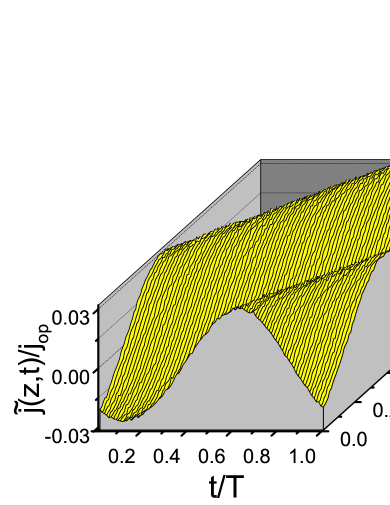
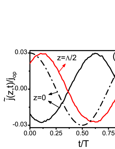
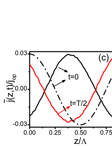
Figure 1: (a): Alternating current ${\tilde{j}}(z,t)$ normalized to the characteristic current, $j_{op}=en_{e}p_{op}/m^{*}$. (b): Time dependence of $\tilde{j}$ at a given $z$. (c): Spatial dependence of $\tilde{j}$ at a given $t$. The dash-dotted lines in (b) and (c) show the alternating electric field for comparison. The simulation parameters are $\omega=0.2$ THz, $q=10^{5}$ cm^-1, $T_{0}=30$ K, $F_{0}=3$ kV/cm, $F_{\omega,q}=0.1\times F_{0}$.

We remark that the alternating current $\tilde{j}(z,t)$ exhibits a nearly plane-wave behavior. Figures 1 (b) and (c) allow to compare the spatial and temporal dependencies of the alternating current with those of the wave field ${\tilde{F}}(z,t)$. From these figures one can conclude that between the alternating current and the alternating field there is a phase-shift $\Delta\varphi_{\omega,q}$.

Below we present the obtained results in terms of the complex HF conductivity. Note that since $\sigma_{\omega,q}$ is the linear response to the field in the form of Eq. (1), we will use the following properties:

$$Re[\sigma_{\omega,q}]=Re[\sigma_{-\omega,-q}],\,\,Re[\sigma_{\omega,-q}]=Re[\sigma_{-\omega,q}],$$

$$Im[\sigma_{\omega,q}]=-Im[\sigma_{-\omega,-q}],\,\,Im[\sigma_{\omega,-q}]=-Im[\sigma_{-\omega,q}].$$

Due to these relationships, we will present the result only for $q>0$ while $\omega$ will take both positive and negative values.

III Frequency and wavevector dispersions of the HF conductivity

The obtained HF conductivity, $\sigma_{\omega,q}$, is dependent on the frequency, $\omega$, and the wavevector, $q$, i.e. both temporal and spatial dispersions of the HF conductivity are important.

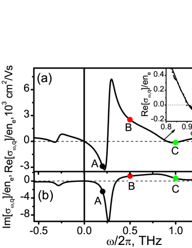
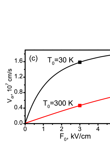
Figure 2: Spectrum of the high-frequency conductivity of the drifting electron gas (solid lines). (a): $Re[\sigma_{\omega,q}]$. (b): $Im[\sigma_{\omega,q}]$. The parameters $F_{0}$, $q$, $T_{0}$ are the same as in Fig. 1. In the inset of panel (a): magnified high-frequency region of interest. Dashed-dotted lines are obtained at $F_{\omega,q}=0.015\times F_{0}$. (c): steady-state dependencies of the drift velocity vs electric field.

A typical spectral dependence of the HF conductivity in the THz frequency range for the drifting electron gas is illustrated in Fig. 2 for a given $|q|$. In this and other figures we show the ratio $\sigma_{\omega,q}/en_{e}$, which is the specific conductivity per one electron comment-1 . Comparing the presented results for the frequency regions $\omega>0$ and $\omega<0$, we see that the drift of the electrons in the stationary field leads to a strong non-reciprocal effect in the dynamic conductivity: indeed a change of the sign of $q$ (which is equivalent to a change of the sign of $\omega$ keeping $q$ unchanged) strongly modifies the frequency dependence of the HF conductivity. This corresponds to essentially different responses of the electron gas to the electric field waves propagating along and against the electron drift.

Another remarkable feature of the frequency dispersion of the HF conductivity of the drifting electrons is nonmonotonous behavior of both $Re[\sigma_{\omega,q}]$ and $Im[\sigma_{\omega,q}]$ with a set of ”frequency windows”, where the real part of the HF conductivity, $Re[\sigma_{\omega,q}]$, becomes negative. To illustrate the importance of such frequency windows, we consider the density of the electric power received by the electrons from the alternating field, ${\cal P}={\tilde{j}}(z,t)\times{\tilde{F}}(z,t)$. Using Eqs. (11) from Appendix we obtain for the time- and space-averaged power: $\langle{\cal P}\rangle=\frac{1}{2}\overline{\sigma}_{\omega,q}F_{\omega,q}^{2}\cos(\Delta\varphi_{\omega,q})=\frac{1}{2}Re[\sigma_{\omega,q}]F_{\omega,q}^{2}$. As mentioned above, the dissipative electron motion generates an alternating current with a phase shift, $\Delta\varphi_{\omega,q}$, with respect to the external alternating field. This phase shift is responsible for attenuation/amplification of the external alternating signal: if $\Delta\varphi_{\omega,q}$ is such that $\cos(\Delta\varphi_{\omega,q})>0$, the electrons dissipate the electrical power, if $\cos(\Delta\varphi_{\omega,q})<0$ (i.e. $Re[\sigma_{\omega,q}]<0$) the electrons supplies the power to the alternating field at the expense of the stationary field and current: this means that an amplification of the external field will take place. In the case of Fig. 2, for the frequencies $0.2$ and $1$ THz indicated by the points $A$ and $C$, $\cos(\Delta\varphi_{\omega,q})<0$ and the amplification is obtained, while for the frequency $0.5$ THz (point B), $\cos(\Delta\varphi_{\omega,q})>0$ and the field $\tilde{F}$ is attenuated.

The physical explanations of the appearance of the negative HF conductivity, $Re[\sigma_{\omega,q}]$, are different for the low frequency window and the windows at higher frequencies. The low-frequency window is characterized by a large effect of the negative HF conductivity: it can be treated as a manifestation of the well known Cherenkov effect i.e. an amplification of a wave by electrons drifting with velocity exceeding the phase velocity of this wave. The Cherenkov amplification occurs only for waves propagating along the direction of the electron drift. For example, at $\omega/2\pi=0.2$ THz and $q=10^{5}$ cm^-1 corresponding to the point A in Fig. 2, the phase velocity, $\omega/q$, is equal to $1.2\times 10^{7}$ cm/s, while calculations give a drift velocity $V_{dr}=1.6\times 10^{7}$ cm/s at the stationary field $F_{0}=3$ kV/cm (see Fig. 2(c)). The Cherenkov effect in the frequency dependent HF conductivity with a spatial dispersion is of general character. The dependence of this effect on the wavevector $q$ and a widening of the corresponding window are illustrated in Fig. 3. We remark that the treatment of this effect can be made even in the framework of the simplified space-dependent hydrodynamic model. However, this treatment leads to the divergence of $\sigma_{\omega,q}$ at $\omega=V_{dr}q$. In contrast, the Monte Carlo method provides a finite results for $\sigma_{\omega,q}$ and the correct determination of the frequency window of the Cherenkov effect.

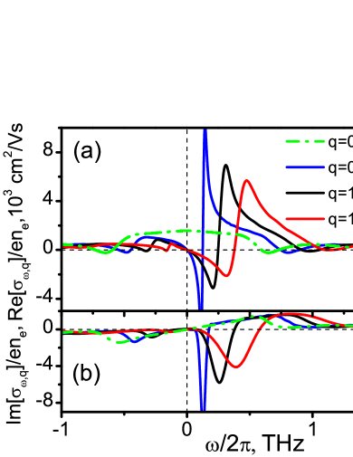
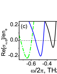
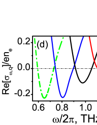
Figure 3: Spectra of the high-frequency conductivity of the drifting electron gas at three different wave vectors $q=0.5,\,1,\,1.5\times 10^{5}$ cm^-1 (curves 1, 2, 3, respectively). (a): $Re[\sigma_{\omega,q}]$. (b): $Im[\sigma_{\omega,q}]$. Dash-dotted curves are for $\sigma_{\omega,0}$. The panels (c) and (d) show the magnified frequency dependencies $Re[\sigma_{\omega,q}]$ for the windows related to the space-dependent OPTT resonance. Results are presented for $T_{0}=30$ K and $F_{0}=3$ kV/cm.

The windows with $Re[\sigma_{\omega,q}]<0$ at higher frequencies are characterized by a smaller, but noticeable, effect on the negative HF conductivity (see also the panels 3(c) and  3(d)). The physical reason of this effect is the space-dependent OPTT resonance, when the electrons oscillate in the nearly-streaming regime in real and momentum spaces resonantly with the space- and time-dependent electric field. The space-dependent OPTT resonance can occur at both signs of $q$, i.e., for the electric wave propagating along as well as against the electron drift. At increasing wavevector $q$, these frequency windows are shifted by the factor $V_{dr}|q|$, as seen from Fig. 3. The amplitudes of the negative HF conductivity under the space-dependent OPTT resonance are about one order of magnitude smaller than in the Cherenkov regions.

As seen from Fig. 3 (a) these resonances vanish with the increasing of the wavevector $q$. The spectra of $Im[\sigma_{\omega,q}]$ also exhibit a nontrivial behavior (see Fig. 3 (b)). To understand the differences between the negative HF conductivity of Cherenkov-type and under the OPTT resonance, we analyzed the dynamics of the electron gas in both real and momentum spaces. Such dynamics can be described through the spatial and temporal dependencies of the average electrons density with given longitudinal $P_{z}$ and transversal $P_{\perp}$ momenta with respect to the electric field direction. To illustrate the obtained results, here we present the density of the electrons with $P_{\perp}(P_{x},P_{y})=0$ and a given energy $\epsilon=P_{z}^{2}/2m^{*}$ in the form:

$${\tilde{n}}(\epsilon,z,t)={\tilde{n}}_{\omega,q}(\epsilon)\cos(qz-\omega t+\Delta\varphi_{\omega,q}(\epsilon))\,,$$ (2)

where ${\tilde{n}}_{\omega,q}(\epsilon)$ and $\Delta\varphi_{\omega,q}(\epsilon)$ have been obtained by the Monte Carlo simulations. In Fig. 4 the dependence of ${\tilde{n}}(\epsilon,z,t)$ on $\epsilon$ is shown at a given spatial coordinate $z$ for two values of the frequency corresponding to the windows with the Cherenkov effect (Fig. 4 (a)) and the OPTT resonance (Fig. 4 (b)).

From Eq. (2) and Fig. 4 (a) it follows that in the Cherenkov frequency window the alternating field of Eq. (1) induces a traveling wave of the electron concentration in the real space and a kind of standing wave in the energy/momentum space. In the Fig. 4 (c), the phase shift $\Delta\varphi(\epsilon)$ corresponding to the Cherenkov frequency window is presented: for most of the electrons having energy $\epsilon<\hbar\omega_{op}$ (the so-called passive region) this phase shift exceeds $\pi/2$, thus, according to the above analysis, these electrons amplify the external electric wave. The minority of electrons with energy $\epsilon>\hbar\omega_{op}$ (the so-called active region) have a phase shifts smaller than $\pi/2$ and contributes to the absorption of the electric wave.

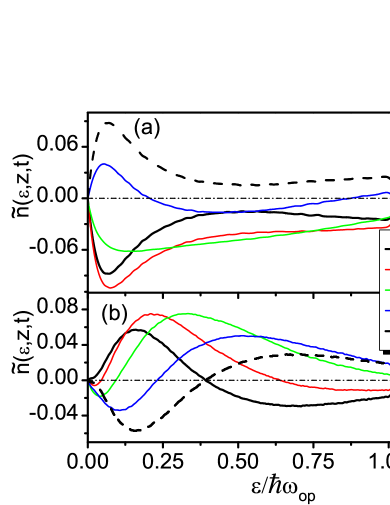
Figure 4: Electron density defined by Eq. (2) as a function of the energy, $\epsilon$, at a given coordinate, $z=0$, and different moments of time $t=0,T/10,T/4,2T/5,T/2$ . (a): $\omega/2\pi=0.2$ THz; (b): $\omega/2\pi=1$ $THz$. The panels (c) and (d) show the energy dependencies of the phase shift, $\Delta\varphi(\epsilon)$ for the case of $\omega/2\pi=0.2$ THz and $\omega/2\pi=1$ THz, respectively. For both panels $q=10^{5}$ cm^-1. Other parameters are the same as in Fig. 3.

In the frequency windows corresponding to the OPTT resonance (Fig. 4 (d)), the electric wave of Eq. (1) is accompanied by oscillations of the electron distribution in the form of traveling waves in both the real and the energy/momentum spaces. The Fig. 4 (d) shows that the phase shift of these oscillations varies from $\pi/2$ to $-\pi$ depending on the electron energy. As a consequence, only high-energy electrons in the passive region $\epsilon<\hbar\omega_{op}$ amplify the external wave. The temporal dynamics of the electron distribution in the active region ($\epsilon>\hbar\omega_{op}$) is similar to that of the Cherenkov frequency window. These results qualitatively explain the distinction of the effects of the negative HF conductivity for the Cherenkov and OPTT resonance frequency windows.

A similar behavior of the spectra of the HF conductivity with the wavevector dependence was obtained using an approximate solution of the Boltzmann transport equation for two-dimensional electron gas in a polar materialKorotyeyev .

IV Discussion

For observation of the negative HF conductivity effects of the Cherenkov and OPTT resonance types, low lattice temperatures are favorable. The Cherenkov effect is less sensitive to the temperature and exists even at $300$ K as illustrated in Fig. 5, though it is realized in a narrower frequency region, because of a smaller drift velocity, $V_{dr}\approx 0.5\times 10^{7}$ cm/s (see Fig. 2(c)) at $F_{0}=3$ kV/cm. It is clear that at room temperature this effect also is less pronounced than at low temperatures (compare with Figs. 3). The OPTT resonances are present only at low temperatures, typically lower than nitrogen temperature, i.e. $T_{0}\leq 77$ K.

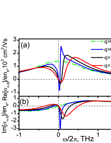
Figure 5: The same as in Fig. 3 for $T_{0}=300\,K$.

For the given parameters of the GaN crystal and temperature, the HF conductivity is dependent on two quantities: $\omega$ and $q$. Therefore, to characterize the negative HF conductivity effect and possible amplification of an external wave, one can use the $\{\omega,q\}$-plane and plot the set of isolines corresponding to certain values of $Re[\sigma_{\omega,q}]$. Such a mapping is presented in Fig. 6 for $Re[\sigma_{\omega,q}]\leq 0$ at $T_{0}=30$ K and $300$ K. In particular, the isolines corresponding to $Re[\sigma_{\omega,q}]=0$ separate the $\{\omega,q\}$-regions with negative HF conductivity. For the case of the Cherenkov effect, this region is the unlimited sector between the lines $\omega=0$ and $\omega=V_{dr}q$ at $q>0$. For $T_{0}=30$ K and wavevectors $q\leq 2\times 10^{5}$ cm^-1, the negative HF conductivity occurs in the frequency range $0\div 0.45$ THz. In this frequency range the specific negative HF conductivity can reach values of several thousands of cm²/Vs. For $T_{0}=300$ K, the negative HF conductivity values are of the order of several hundreds of cm²/Vs at frequencies lower than $0.15$ THz. Such a suppression of the Cherenkov effect is due to the decrease of the drift velocity at room temperature.

From Fig. 6, one can see that at $T_{0}=30$ K the spatially dependent OPTT resonance and the negative HF conductivity occur in a wide frequency range from 0.6 to 1.2 THz, when the wavevector varies from $0$ to $1.5\times 10^{6}$ cm^-1. At $q=0$, i.e. in the absence of space dependence of the alternating field of Eq.(1), the negative HF conductivity due to the OPTT resonance is possible only in the narrow frequency range of $0.6\div 0.73$ THz. However, the maximum effect is realized at $q=0$ and $\omega/2\pi=0.65$ THz where $Re[\sigma_{\omega,q}/en_{e}]=-230$ cm²/Vs.

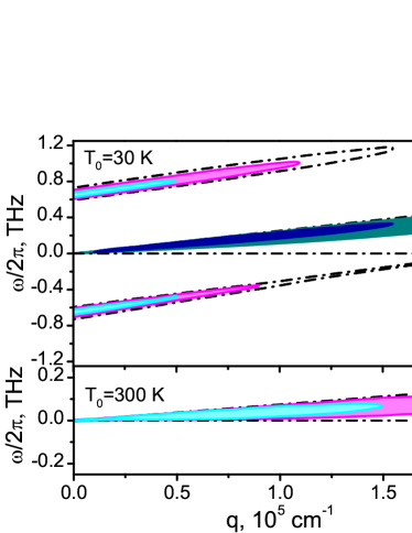
Figure 6: Contour plots of $Re[\sigma_{\omega,q}]/en_{e}$ in the $\{\omega,q\}$-plane. Curves 1, 2, 3, 4 and 5 restrict the regions of $\{\omega,q\}$, where $Re[\sigma_{\omega,q}]/en_{e}<0,\,-100,\,-200,\,-1000,\,-2000$ cm²/Vs, respectively. $F_{0}=3$ kV/cm.

We suggest that the discovered features associated with the response of the drifting electrons to high-frequency and spatially nonuniform electromagnetic fields are of general character. Indeed, similar features of the electron response were found for different drifting electron systems: two-dimensional electrons Kempa ; Mikhailov , electrons in graphene strips Mikhailov-Gr and two-dimensional electrons in GaN quantum wells Korotyeyev . Very recently, HF-sigma-2018 an oscillation behavior of the HF conductivity and frequency windows with its negative values were found and explained in the collisionless limit for structure with GaAs quantum wells. The important condition to obtain these effects is an anisotropy of the distribution function of the drifting electrons. For example, in GaAs quantum wells, electric fields of order of a few kV/cm (0.5 - 2 kV/cm) induce enough anisotropic distribution of electrons to provide a negative $Re[\sigma(\omega,q)]$ in the THz frequency range at $q$ of the order of $10^{5}$ cm^-1 (see Ref. HF-sigma-2018 ).

The dependence of $\sigma_{\omega,q}$ on the wavevector $q$, i.e. the spatial dispersion, becomes particularly important for samples with submicron- and nanosized structuring. Indeed, a plane electromagnetic wave illuminating a nonuniform sample induces electric field components varying both in space and time, which interact with the electrons. The spatial dependence of these field components is defined by the characteristic scales of the structuring of the sample. Examples of such nonuniform structures are grating-gated semiconductor structures, surface-relief grating, plasmonic and metamaterial nanodevices, etc. (see review in Ref. [Plasmonics, ]). These structures can be used for different applications, including detecting and emitting devices of far-infrared and terahertz radiation.

The knowledge of $\sigma_{\omega,q}$ is also important for the electrodynamic modeling of the high-frequency characteristics such as transmission, reflection and absorption. Moreover, the spatially dependent high-frequency conductivity is directly related to the plasmonic properties of the electron gas.

In conclusion, using Monte Carlo simulations of the electron motion in stationary and space- and time-dependent electric fields, we have determined the wavevector dependence of the HF conductivity, $\sigma_{\omega,q}$, for compensated GaN samples. In particular, we have found that the spatially dependent HF conductivity of the drifting electrons can be negative under stationary electric field of moderate amplitude ($2..5$ kV/cm). This effect is realized in some frequency windows. The physics underlying this negative HF conductivity is different for the low-frequency and the high-frequency windows. The low-frequency windows are due to the Cherenkov mechanism. The detailed analysis has shown that the alternating field induces a traveling wave of the electron concentration in the real space and a kind of standing wave in the energy/momentum space. The high-frequency windows are explained by the OPTT resonances. For this case the alternating field is accompanied by oscillations of the electron distribution in the form of traveling waves in both the real and the energy/momentum spaces. For the observation of both types of negative HF conductivity effects, low lattice temperatures are favorable. Finally, the negative HF conductivity can be used to amplify electromagnetic waves at the expense of the energy of the stationary field and current.

V Acknowledgement

This work is supported by the Ministry of Education and Science of Ukraine (Project M/24-2018) and German Federal Ministry of Education and Research (BMBF Project 01DK17028).

VI Appendix

An electron subjected to the electric field $F_{0}+\tilde{F}(z,t)$ and undergoing scatterings by defects and phonons moves along a complex trajectory in the three-dimensional real space. To find the alternating electric current induced by the field $\tilde{F}(z,t)$, we analyze the projection of the electron trajectory along the $OZ$-axis, i.e. the dependence $z_{e}(t)$ with $z$ being the electron coordinate and $t\geq 0$, i.e. the projection $z_{e}(t)$ lies in the right-half of the $\{t,z\}$-plane. We discretize this half-plane with rectangular cells of height $\Lambda=2\pi/q$, and width $T=2\pi/\omega$, where $\Lambda$ and $T$ are the spatial and temporal periods of the field given by Eq. (1). A generic $\{{\cal V}_{t},{\cal V}_{z}\}$-cell is defined as

$$T{\cal V}_{t}<t_{{\cal V}_{t}}<T({\cal V}_{t}+1),\,\Lambda{\cal V}_{z}<z_{{\cal V}_{z}}<\Lambda({\cal V}_{z}+1)$$

with ${\cal V}_{t}=0,1,2...N_{T}-1$ and ${\cal V}_{z}=0,\pm 1,\pm 2...$. Here $N_{T}$ indicates the number of simulated time periods. Then we divide each cell into small meshes of sizes $T/M_{T}\times\Lambda/M_{Z}$, so that the $\{\nu_{t},{\cal V}_{t};\nu_{z},{\cal V}_{z}\}$-mesh is determined as:

$$T({\cal V}_{t}+\nu_{t}/M_{T})<t_{{\cal V}_{t},\nu_{t}}<T({\cal V}_{t}+(\nu_{t}+1)/M_{T})$$

$$\Lambda({\cal V}_{z}+\nu_{z}/M_{Z})<z_{{\cal V}_{z},\nu_{z}}<\Lambda({\cal V}_{z}+(\nu_{z}+1)/M_{Z})$$

with $\nu_{t}=0,1,2,...M_{T}-1$ and $\nu_{z}=0,1,2,...M_{Z}-1$; the numbers $M_{Z},\,M_{T}$ are integer and large. Note that the temporal and spatial periodicities of the external signal imply that all electron characteristics should have the same periodicity. This means that any mesh corresponding to the same spatial phase, $qz$, and temporal phase, $\omega t$, are equivalent within a factor $2\pi\times\,integer$

The calculations of the electron current requires the simulation of electron trajectory also in the momentum space. Here, we restrict ourself to the electron current component in the direction of the applied electric field thus we discretize the momentum space along the OZ-direction as follows:

$$-P_{max}(1-(\nu_{p}+M_{P})/M_{P})<P_{z,\nu_{p}}<-P_{max}\times$$

$$(1-(\nu_{p}+1+M_{P})/M_{P})$$

where $\nu_{p}=-M_{P}...M_{P}-1$ and $P_{max}$ is selected so that the probability of finding an electron with momentum $P_{z}=P_{max}$ and higher is negligible.

To follow the periodic electron motion induced by the alternating field during the simulation of a sufficiently long trajectory in the $\{z,P_{z}\}$-phase space, we count in each $\{\nu_{t},\nu_{z}\}$-mesh the number of electron appearances ${\cal N}_{\nu_{p},\nu_{t},\nu_{z}}$ in all meshes with equivalent spatial, $qz_{\nu_{z}}$, and temporal, $\omega t_{\nu_{t}}$, phases and recorded the corresponding momentum projection, $P_{z,\nu_{p},\nu_{t},\nu_{z}}$. Having these data we can calculate the spatial- and temporal- dependence of the current density, $j_{z}(z_{\nu_{z}},t_{\nu_{t}})$, within one spatial and temporal period as:

$$J_{z}(z_{\nu_{z}},t_{\nu_{t}})=-\frac{e}{m^{*}}n_{e}M_{T}M_{z}\sum_{\nu_{p}}P_{z,\nu_{p},\nu_{t},\nu_{z}}W_{\nu_{p},\nu_{t},\nu_{z}},$$ (3)

where $W_{\nu_{p},\nu_{t},\nu_{z}}$ is the probability to find electron in the $\{\nu_{t},\nu_{z}\}$-mesh with momentum projection, $P_{z,\nu_{p}}$ that is $W_{\nu_{p},\nu_{t},\nu_{z}}={\cal N}_{\nu_{p},\nu_{t},\nu_{z}}/\sum_{\nu_{p},\nu_{t},\nu_{z}}{\cal N}_{\nu_{p},\nu_{t},\nu_{z}}$.

By averaging Eq. (3) with respect to the coordinate and time we can obtain the steady-state current density, $J_{z,0}(F_{0})$,

$$J_{z,0}=-\frac{e}{m^{*}}n_{e}\sum_{\nu_{p},\nu_{t},\nu_{z}}P_{z,\nu_{p},\nu_{t},\nu_{z}}W_{\nu_{p},\nu_{t},\nu_{z}},$$ (4)

as well as different Fourier harmonics of the alternating current, $\tilde{j}(z,t)=J_{z}(z,t)-J_{z,0}$. For example, the first-order Fourier harmonic describing the linear response can be calculated as:

$$\left[\begin{array}[]{c}Re[j_{\omega,q}]\\ Im[j_{\omega,q}]\end{array}\right]=-\frac{2e}{m^{*}}n_{e}\!\!\sum_{\nu_{p},\nu_{t},\nu_{z}}P_{z,\nu_{p},\nu_{t},\nu_{z}}W_{\nu_{p},\nu_{t},\nu_{z}}\times\!$$ (7)

$$\left[\begin{array}[]{c}\cos(qz_{\nu_{z}}-\omega t_{\nu_{t}})\\ \sin(qz_{\nu_{z}}-\omega t_{\nu_{t}})\end{array}\right]$$ (10)

The calculated values of $J_{z,0}$, $Re[j_{\omega,q}]$ and $Im[j_{\omega,q}]$ parametrically depends on the magnitude of the stationary field $F_{0}$. In the small-signal limit, $F_{\omega,q}/F_{0}<<1$, the ratios of $Re[j_{\omega,q}]/F_{\omega,q}$ and $-Im[j_{\omega,q}]/F_{\omega,q}$ become independent of the alternating field amplitude, $F_{\omega,q}$ and give the real, $Re[\sigma_{\omega,q}]$, and imaginary, $Im[\sigma_{\omega,q}]$, parts of the complex HF conductivity, respectively. In this case the alternating current $\tilde{j}(z,t)$ has the almost harmonic form:

$$\tilde{j}(z,t)\approx{\overline{\sigma}}_{\omega,q}F_{\omega,q}\cos(qz-\omega t+\Delta\varphi_{\omega,q})\,,$$ (11)

where ${\overline{\sigma}}_{\omega,q}=\sqrt{Re[\sigma_{\omega,q}]^{2}+Im[\sigma_{\omega,q}]^{2}}$ and the phase shift between the alternating field and the current is $\Delta\varphi_{\omega,q}=\arctan(Im[\sigma_{\omega,q}]/Re[\sigma_{\omega,q}])$.

To prove the accuracy of the simulation, we checked the convergence of the calculations varying the numbers and sizes of the cells and the meshes used in the simulation of space- and time dependent electron transport.

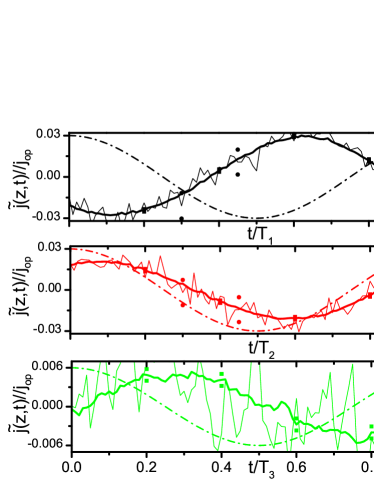
Figure 7: Time dependencies of the alternating current calculated for $N_{T}=10^{6}$ (thin curve) and $N_{T}=10^{8}$ (thick curve). (a), (b) and (c) correspond to the frequencies $\omega_{A},\,\omega_{B}$ and $\omega_{C}$ presented in the text. The time is normalized to the corresponding period of the alternating field whose time-dependence is shown by the dash-dotted lines. Results are presented for $z=0$ and $F_{\omega,q}=0.1\times F_{0}$.

As an example, Fig. 7 presents the alternating currents obtained using different numbers of the temporal period, $N_{T}$, for three frequencies (marked by points in Fig.2) of the field $\tilde{F}$. For the used mesh sizes, $\Lambda/M_{Z},\,T/M_{T}$ we set $M_{Z}=M_{T}=100$. As seen from Fig. 7, the two curves calculated for $N_{T}=10^{6}$ and $N_{T}=10^{8}$ coincide within a small statistical error for two cases of low frequencies $\omega_{A}/2\pi=0.2$ and $\omega_{B}/2\pi=0.5$ THz (Fig. 7 (a) and (b)). At higher frequency, $\omega_{C}/2\pi=1$ THz, only the use of $N_{T}=10^{8}$ is sufficient to obtain a satisfactory accuracy of the computations (Fig. 7 (c)).

By varying the field amplitude $F_{\omega,q}$ from $0.015\times\,F_{0}$ to $0.1\times\,F_{0}$, we found that the ratio $j_{\omega,q}/F_{\omega,q}$ does not depend on the amplitude $F_{\omega,q}$ for $F_{\omega,q}\leq 0.1\,F_{0}$.

In the previous sections, we have presented results for the $N_{T}=10^{8}$, $M_{T}=100$, $M_{Z}=100$ and $F_{\omega,q}/F_{0}=0.1$. For such parameters the relative error of the calculation of $\sigma_{\omega,q}$ does not exceed $1\%$ in the range of investigated frequencies and wavevectors. The computational parameters related to the momentum space were $M_{P}=500$ and $P_{max}=3\times p_{op}$.

References

- (1) W. Shockley, Bell Syst. Tech. J. Eng. R 30, 990 (1951).
- (2) Y. Katayama and K. F. Komatsubara, Phys. Rev. Lett. 19, 1421 (1967).
- (3) P. F. Lu, D. C. Tsui, and H. M. Cox, Phys. Rev. Lett. 54, 1563 (1985).
- (4) T. W. Hickmott, P. M. Solomon, F. F. Fang, F. Stern, R. Fischer, and H. Morkoc, Phys. Rev. Lett. 52, 2053 (1984). L. Eaves, P. S. S. Guimaranes, B. R. Snell, D. C. Taylor and K. E. Singer, Phys. Rev. Lett. 55, 262 (1985).
- (5) P. F. Lu, D. C. Tsui, and H. M. Cox, Phys. Rev. B 35, 9659 (1987).
- (6) V. Gruzinskis, P. Shiktorov, E. Starikov, L. Reggiani, L. Varani, and J. C. Vaissiere, Semicond. Sci. Technol. 19, S173 (2004).
- (7) A. Iñiguez-de-la-Torre, J. Mateos, and T. Gonzalez J. Appl. Phys. 107, 053707 (2010).
- (8) Special Issue on Far-Infrared Semiconductor Lasers, edited by E. Gornik and A. A. Andronov, Opt. Quantum Electron. 23(2), S111 S360 (1991).
- (9) E. Starikov, P. Shiktorov, V. Gruzinskis, L. Varani, et al., J. Nanoelectron. Optoelectron 2, 11 (2007); E. Starikov, P. Shiktorov, V. Gruzinskis, L. Varani, C. Palermo, J. F. Millithaler, and L. Reggiani, J. Phys.: Condens. Matter 20, 384209 (2008).
- (10) V. V. Korotyeyev, V. A. Kochelap, K. W. Kim and D. L. Woolard, Appl. Phys. Lett. 82, 2643 (2003). K. W. Kim, V. V. Korotyeyev, V. A. Kochelap, A. A.Klimov and D. L. Woolard, J. Appl. Phys. 96, 6488 (2004).
- (11) J. T. Lu, J. C. Cao and S. L. Feng, Phys. Rev. B 73, 195326 (2006). J. T. Lu and J. C. Cao, Semicond. Sci. Technol. 20, 829 (2005).
- (12) E. Starikov, P. Shiktorov, V. Gruzinskis, A. Dubinov, V. Aleshkin, L. Varani, C. Palermo, L. Reggiani, J. Comput. Electron. (2007) 6, 45 (2007). P. Shiktorov, E. Starikov, V. Gruzinskis, L. Varani, C. Palermo, J-F. Millithaler and L. Reggiani, Phys. Rev. B 76, 045333 (2007).
- (13) A. Akturk, N. Goldsman, G. Pennington and A. Wickenden, Phys. Rew. Lett. 98, 166803 (2007); A. Akturk, N. Goldsman and G. Pennington, J. Appl. Phys. 102, 073720 (2007); A. Akturk, G. Pennington, N. Goldsman, and A. Wickenden, IEEE Trans. Nanjtech. 6, 469 (2007).
- (14) E. Vorob ev, S. N. Danilov, V. N. Tulupenko, and D. F. Firsov, JETP Lett. 73, 219 (2001).
- (15) V. V. Korotyeyev, V. A. Kochelap, and L. Varani, J. Appl. Phys. 112, 083721 (2012). The solution of the Boltzmann transport equation was obtained approximately, using Baraff stylization [V. V. Korotyeyev, V. A. Kochelap, K. W. Kim, D. L. Woolard, Appl. Phys. Lett., 82, 2643 (2003)] of distribution function in momentum space.
- (16) W. Fawcett, A.D. Boardman and S. Swain, J. Chem. Solids 31, 1963-1990 (1970).
- (17) C. Jacoboni and L. Reggiani, Rev. Mod. Phys. 55 (3), 645-705 (1983).
- (18) G I Syngayivska and V V Korotyeyev, Ukr. J. Phys. 58(1) 40-55 (2013).
- (19) G I Syngayivska, V V Korotyeyev and V A Kochelap, Semicond. Sci. Technol. 28 035007 (2013).
- (20) J. Zimmerman, Y. Leroy and E. Constant, J. Appl. Phys. 49(7), 3378-3383 (1978).
- (21) Though the dimension of is , this ratio is not an electron mobility.
- (22) K. Kempa, P. Bakshi, H. Xie, W. L. Schaich Phys. Rev. B, 47(8), 4532 (1993).
- (23) Mikhailov S A, Appl. Phys. 2, 65 108 (1999).
- (24) S. A. Mikhailov, N. A. Savostianova, A. S. Moskalenko, Phys. Rev. B 94, 035439 (2016).
- (25) V. V. Korotyeyev, V. A. Kochelap, S. Danylyuk, and L. Varani, Appl. Phys. Lett. 113, 041102 (2018).
- (26) Ho-Jin Song, Tadao Nagatsuma, Handbook of Terahertz Technologies: Devices and Applications, CRC Press, 2015.