Convergence of metadynamics: discussion of the adiabatic hypothesis

Abstract

By drawing a parallel between metadynamics and self interacting models for polymers, we study the longtime convergence of the original metadynamics algorithm in the adiabatic setting, namely when the dynamics along the collective variables decouples from the dynamics along the other degrees of freedom. We also discuss the bias which is introduced when the adiabatic assumption does not holds.

Introduction

The objective of this work is to discuss the long time properties of the metadynamics algorithm [LP02], by exploiting in particular similarities between metadynamics and self interacting stochastic models for polymers [TV11, TTV12].

The metadynamics algorithm consists in evolving a random walker and adding a penalty over already visited states in order to escape from metastable states. More precisely, one considers a process $(Q_{t})_{t\geq 0}$ following originally a dynamics with invariant probability measure $\pi(dq)=\exp(-\beta V(q))\,dq$ (where $V$ is the potential energy function and $\beta>0$ is the inverse temperature). One is also given a so-called collective variable $\xi$ which is a function of the position $q$ giving a low-dimension description of the state of the system (say for simplicity that $\xi$ is with values in the one-dimensional torus). An important quantity related to the target distribution $\pi$ and the collective variable $\xi$ is the so-called free energy [LRS10] defined by

$$\exp(-\beta F(z))dz=\xi_{\#}\pi$$ (1)

where $\xi_{\#}\pi$ denotes the image of the measure $\pi$ by $\xi$. As the walker $(Q_{t})_{t\geq 0}$ evolves, the dynamics is modified in order to target at time $t$ a biased measure $\pi_{t}$, where

$$\frac{d\pi_{t}}{d\pi}(q)\varpropto\exp\left(-\beta\int_{0}^{t}\delta^{\epsilon}\left(\xi(Q_{s})-\xi(q)\right)\,ds\right).$$ (2)

and $\delta^{\epsilon}$ is a smooth approximation of the Dirac delta function. The aim of metadynamics is twofold: (i) to converge more quickly to an equilibrium state than for the original unbiased dynamics; (ii) to obtain in the long-time limit an estimate of the free energy as the opposite of the penalty term $\Psi_{t}:z\mapsto\int_{0}^{t}\delta^{\epsilon}\left(\xi(Q_{s})-z\right)\,ds$. The function $\Psi_{t}$ records the already visited values of $\xi$: intuitively, one could think of $\Psi_{t}$ as “computational sand filling the free energy wells”. Concerning the long-time convergence, if one keeps on penalizing the already visited states with the same penalization strength all along the trajectory, as in (2), the penalty term $\Psi_{t}$ cannot converge. Two ideas have been proposed in the literature to overcome this difficulty. The first idea is averaging, see for example [LG08, Section 3.1]: this consists in considering the long-time limit of the time average of the penalizing term: $\frac{1}{t}\int_{0}^{t}\Psi_{s}(z)\,ds$. The second idea is vanishing adaption: this consists in reducing the penalization strength to zero in the long-time limit, namely add a multiplicative factor $\alpha(s)$ in front of $\delta^{\epsilon}\left(\xi(Q_{s})-\xi(q)\right)$ in (2), where $\alpha(s)$ goes to $0$ as $s\to\infty$. The so-called well-tempered metadynamics [BBP08] is a version of metadynamics with a vanishing penalization mechanism where $\alpha(s)$ scales as a constant over $s$. We refer to [DPV14, For+17, For+18] for convergence analysis of well-tempered metadynamics using tools from stochastic approximation algorithms. The difficulty of approaches with vanishing adaption is to decide at which rate the penalization strength should decrease: if it vanishes too fast, the system may remain stuck in a metastable state; if it vanishes too slowly, large fluctuations of the penalizing term affect the accuracy of the estimator of the free energy, see for example [For+18] for discussion.

We are interested here in the averaging approach. This technique has been used in particular in the context of biased exchange metadynamics, see for example [Gha+12, Baf+12]. As will be explained below (see also [LG08]), the averaging approach is biased in nature: $\frac{1}{t}\int_{0}^{t}\Psi_{s}(z)\,ds$ will not converge in the long time limit to $-F(z)$ (up to an additive constant), except in the so-called adiabatic case, namely when $(\xi(Q_{s}))_{s\geq 0}$ follows an autonomous Markov dynamics [ILP03, BLP06]. The adiabatic case is equivalent to a situation in which the original dynamics is with values in ${\rm Ran}(\xi)$ and directly samples $\exp(-\beta F(z))\,dz$, so that one can consider simply the identity as a collective variable. The fact that the averaging approach is biased is clearly a drawback, but one interest compared to a vanishing adaption method (such as well-tempered metadynamics) is that one can look at the way the penalization term $\Psi_{t}$ evolves in time in order to assess if the underlying adiabatic assumption is satisfied: if hidden metastabilities have not been taken into account in the choice of $\xi$, one observes some kind of periodic behavior of $\Psi_{t}$ in time. This will be illustrated below on numerical examples.

The objective of this work is twofold. First, we present in Section 1 some theoretical results on the unbiasedness of the averaging approach in the case of adiabatic separation, for two versions of metadynamics: a dynamics in continuous state space where we built on previous results from [BCG15, BG17] and a dynamics in discrete state space — the proof of the results in this case are based on [TV11] and given in Section 3. Second, we give some theoretical and numerical evidence of the fact that the average of the penalty term yields a biased estimator of minus the free energy for non adiabatic cases in Section 2.

1 Consistency of metadynamics with adiabatic separation

In this section, we prove the convergence of the average in time of the penalty term to minus the free energy, in the adiabatic case, on prototypical dynamics in continuous state space (Section 1.1) and in discrete state space (Section 1.2)

1.1 A model in continuous state space

1.1.1 Convergence results

The results of this section can be seen as a formalization of the pioneering work [BLP06], where a similar model is considered.

Let us first introduce the (non-penalized) one-dimensional overdamped Langevin dynamics which samples $Z^{-1}\exp(-\beta F(z))\,dz$:

$$dZ^{OL}_{t}=-F^{\prime}(Z^{OL}_{t})\,dt+\sqrt{2\beta^{-1}}dB_{t},$$ (3)

where $\beta>0$ is the inverse temperature and $(B_{t})_{t\geq 0}$ is a Brownian motion. Compared to the setting presented in the introduction, we are in the case of a so-called adiabatic separation between the dynamics on $Z^{OL}_{t}=\xi(Q_{t})$ and the dynamics of the other degrees of freedom: the dynamics on $Z^{OL}_{t}$ is closed and Markovian, and thus, the drift in (3) is minus the derivative of the free energy $F$, and the invariant measure is then $Z^{-1}\exp(-\beta F(z))\,dz$. This dynamics will typically remain trapped in free energy wells. As explained above, the idea of metadynamics is to penalize already visited states in order to accelerate the sampling. The metadynamics associated with (3) (for a collective variable which is the identity since we are in the adiabatic setting) gives the evolution of the one-dimensional stochastic process $Z_{t}$ and an associated function $\Psi_{t}$, defined formally as follows:

$$\left\{\begin{aligned} dZ_{t}&=-\left(F^{\prime}(Z_{t})+\Psi_{t}^{\prime}(Z_{t})\right)\,dt+\sqrt{2\beta^{-1}}dB_{t},\\ \frac{d\Psi_{t}(z)}{dt}&=\gamma\delta^{\epsilon}(Z_{t}-z),\end{aligned}\right.$$ (4)

where $\Psi_{t}^{\prime}=\frac{d\Psi_{t}}{dz}$ denotes the derivative with respect to $z$, $\gamma>0$ is the so-called deposition rate and $\delta^{\epsilon}$ is a smooth even approximation of the Dirac function. The initial conditions are $(Z_{0},\Psi_{0})$ where $Z_{0}$ is any random variable independent of the Brownian motion $(B_{t})_{t\geq 0}$ and $\Psi_{0}=0$. To give a proper meaning to (4) is not obvious since this is an infinite dimensional stochastic differential equation [DZ14, BCG15]. One aim of this section is actually to exhibit a proper setting where this is well defined, using [BCG15]. For the moment, we argue formally.

In order to simplify the presentation and build on previous results in the literature [TTV12, BCG15, BG17], we assume that $Z_{t}$ lives on the one-dimensional torus $\mathbb{T}$ with period $2\pi$, which amounts to assuming that both $F$ and $\delta^{\epsilon}$ are periodic functions with period $2\pi$. The question we would like to address is the following: Can we prove that $\lim_{t\to\infty}\frac{1}{t}\int_{0}^{t}\Psi_{s}=-F+C$ where $C$ is an irrelevant constant to be made precise?

Let us now introduce

$$\Phi_{t}(z)=\Psi_{t}(z)+F(z)-\frac{1}{2\pi}\int_{\mathbb{T}}F.$$

We add the constant $-\frac{1}{2\pi}\int_{\mathbb{T}}F$ so that $\Phi_{0}$ has zero mean, which will be convenient below to identify the equilibrium measure of the dynamics (notice that only the $z$-derivatives of $\Psi_{t}$ and $\Phi_{t}$ appear in the dynamics). The dynamics (4) can be rewritten as follows:

$$\left\{\begin{aligned} dZ_{t}&=-\Phi_{t}^{\prime}(Z_{t})\,dt+\sqrt{2\beta^{-1}}dB_{t},\\ \frac{d\Phi_{t}(z)}{dt}&=\gamma\delta^{\epsilon}(Z_{t}-z),\end{aligned}\right.$$ (5)

with initial conditions $Z_{0}$ and $\Phi_{0}=F-\frac{1}{2\pi}\int_{\mathbb{T}}F$.

In order to go further, let us now make $\delta^{\epsilon}$ precise. Starting from the relation in distribution sense (for smooth $2\pi$ periodic test functions) $\delta=\frac{1}{2\pi}+\frac{1}{\pi}\sum_{k\geq 1}\cos(k\cdot)$, a possible choice is to consider the truncated Fourier expansion

$$\delta^{\epsilon}(z)=\sum_{k=1}^{N}\cos(kz).$$ (6)

We omit the additive constant $1/(2\pi)$: this is useful in order to keep the normalization $\int_{\mathbb{T}}\Phi_{t}$ to zero as time evolves and thus to obtain a stationary measure for $\Phi_{t}$ (otherwise $\int_{\mathbb{T}}\Phi_{t}$ would evolve linearly in time). Moreover, we forget the multiplicative constant $1/\pi$ since it can be taken into account by modifying $\gamma$. The dynamics (5) then writes:

$$\left\{\begin{aligned} dZ_{t}&=-\Phi_{t}^{\prime}(Z_{t})\,dt+\sqrt{2\beta^{-1}}dB_{t},\\ \frac{d\Phi_{t}(z)}{dt}&=\gamma\sum_{k=1}^{N}\cos(kZ_{t})\cos(kz)+\gamma\sum_{k=1}^{N}\sin(kZ_{t})\sin(kz).\end{aligned}\right.$$ (7)

It is then natural to introduce the Fourier series associated with $\Phi_{t}$ (remember that for all $t\geq 0$, $\int_{\mathbb{T}}\Phi_{t}(z)\,dz=0$):

$$\Phi_{t}(z)=\sum_{k=1}^{\infty}\alpha_{t}^{k}\cos(kz)+\sum_{k=1}^{\infty}\beta_{t}^{k}\sin(kz)$$

where $\alpha_{t}^{k}=\frac{1}{\pi}\int_{\mathbb{T}}\Phi_{t}(y)\cos(ky)\,dy$ and $\beta_{t}^{k}=\frac{1}{\pi}\int_{\mathbb{T}}\Phi_{t}(y)\sin(ky)\,dy$. In the following, we use the notation $\alpha_{t}=(\alpha^{1}_{t},\ldots,\alpha^{N}_{t})$ and $\beta_{t}=(\beta^{1}_{t},\ldots,\beta^{N}_{t})$. Let us define

$$\Pi_{N}^{\perp}(\Phi_{0})(z) =\Phi_{0}(z)-\left(\sum_{k=1}^{N}\alpha_{0}^{k}\cos(kz)+\sum_{k=1}^{N}\beta_{0}^{k}\sin(kz)\right)=\sum_{k=N+1}^{\infty}\alpha_{0}^{k}\cos(kz)+\sum_{k=N+1}^{\infty}\beta_{0}^{k}\sin(kz),$$

the projection of $\Phi_{0}=F(z)-\frac{1}{2\pi}\int_{\mathbb{T}}F$ over the Fourier modes $(\cos(k\cdot),\sin(k\cdot))_{k\geq N+1}$. Notice that since $\Phi_{0}=F-\frac{1}{2\pi}\int_{\mathbb{T}}F$,

$$\Pi_{N}^{\perp}(\Phi_{0})=\Pi_{N}^{\perp}(F).$$

The dynamics (7) can now be rewritten rigorously as the following finite-dimensional stochastic differential equation:

$$\left\{\begin{aligned} dZ_{t}&=\sum_{k=1}^{N}k\left(\alpha^{k}_{t}\sin(kZ_{t})-\beta^{k}_{t}\cos(kZ_{t})\right)\,dt-\Pi_{N}^{\perp}(F)^{\prime}(Z_{t})\,dt+\sqrt{2\beta^{-1}}dB_{t},\\ d\alpha^{k}_{t}&=\gamma\cos(kZ_{t})dt\text{ for all }k\in\{1,\ldots,N\},\\ d\beta^{k}_{t}&=\gamma\sin(kZ_{t})dt\text{ for all }k\in\{1,\ldots,N\},\end{aligned}\right.$$ (8)

with initial condition $Z_{0}$, and $(\alpha^{k}_{0},\beta^{k}_{0})_{k\in\{1,\ldots,N\}}$. Equation (8) gives a proper meaning to the original dynamics (4) for the case $\delta^{\epsilon}$ is defined by (6).

Using techniques from [DMS15], the following result is proven in [BG17]:

Proposition 1.1.

Assume that

$$\Pi_{N}^{\perp}(F)=0.$$ (9)

Then, the Markov process (8) is a positive Harris process and admits a unique invariant probability distribution given as

$$\mu(dz,d\alpha,d\beta)=\frac{dz}{2\pi}\prod_{k=1}^{N}\frac{k^{2}}{2\pi\gamma}\exp\left(-\frac{k\left(\alpha_{k}^{2}+\beta_{k}^{2}\right)}{2\gamma}\right)d\alpha_{k}\,d\beta_{k}.$$

Moreover, one has the following ergodicity results

• for all $f\in L^{1}(\mu)$, $\lim_{t\to\infty}\frac{1}{t}\int_{0}^{t}f(Z_{s},\alpha_{s},\beta_{s})=\int_{\mathbb{T}\times\mathbb{R}^{N}\times\mathbb{R}^{N}}fd\mu$

• there exists $\lambda>0$ such that, for all initial condition $y_{0}=(z_{0},\alpha_{0},\beta_{0})\in\mathbb{T}\times\mathbb{R}^{N}\times\mathbb{R}^{N}$ there exists $C(y_{0})>0$ such that, for all $t\geq 1$,

  $$\|P_{t}(y_{0},dy)-\mu(dy)\|_{TV}\leq C(y_{0})\exp(-\lambda t),$$

  where $P_{t}(y_{0},dy)$ denotes the law of $(Z_{t},\alpha_{t},\beta_{t})$ following the dynamics (8) starting from the initial condition $(Z_{0},\alpha_{0},\beta_{0})=y_{0}$.

As a consequence, one obtains the following corollary.

Corollary 1.2.

Let us consider the dynamics (4) with the choice (6) for $\delta^{\epsilon}$. Under the assumption (9), one has

$$\lim_{t\to\infty}\frac{1}{t}\int_{0}^{t}\Psi_{s}ds=-F+\frac{1}{2\pi}\int_{\mathbb{T}}F.$$

It would be interesting to understand what can be said on the long-time behavior of (8) without the assumption (9).

1.1.2 Discussion and generalization

On the diffusion constant.

As explained in [BG17], the results of Proposition 1.1 hold whatever the diffusion constant: $\sqrt{2\beta^{-1}}$ can be replaced by any positive $\sigma$ in (4), and one still obtains the same limiting behavior. Moreover, for $\sigma=0$ (which actually corresponds to the original metadynamics algorithm in [LP02]), the measure $\mu$ is still invariant for the deterministic dynamical system, but it is not necessarily unique. We refer to [BG17, Theorem 3] where the authors identify infinitely many ergodic measures in the case $N=1$.

More general geometrical setting.

We presented the results in Proposition 1.1 on the one-dimensional torus for simplicity, but they actually hold for $Z_{t}$ with values in any compact Riemanian manifold, the functions $\cos(kz)$ and $\sin(kz)$ being replaced by the eigenfunctions of the Laplace Beltrami operator on the manifold (see [BG17]).

On the infinite dimensional setting.

An infinite-dimensional version of the results of [BG17] is given in [BCG15]. In our context, it can be translated as follows. Let us consider again the dynamics (5), with a function

$$\delta^{\epsilon}(z)=\sum_{k=1}^{\infty}a_{k}\cos(kz)$$ (10)

for some positive sequence $(a_{k})_{k\geq 1}$ such that $\sum_{k=1}^{\infty}(1+k^{2})^{5}a_{k}^{2}<\infty$ (compare with (6)). For example, if $\delta^{\epsilon}$ is a periodic function in the Sobolev space $H^{5}(\mathbb{T})$, then those properties are satisfied. As above, let us introduce the Fourier series for $\Phi_{t}$:

$$\Phi_{t}(z)=\sum_{k=1}^{\infty}\alpha_{t}^{k}\cos(kz)+\sum_{k=1}^{\infty}\beta_{t}^{k}\sin(kz).$$

In this context, the dynamics (8) can be rewritten in the following form:

$$\left\{\begin{aligned} dZ_{t}&=\sum_{k=1}^{\infty}k\left(-\alpha^{k}_{t}(-\sin(kZ_{t}))-\beta^{k}_{t}\cos(kZ_{t})\right)\,dt+\sqrt{2\beta^{-1}}dB_{t},\\ d\alpha^{k}_{t}&=\gamma a_{k}\cos(kZ_{t})dt\text{ for all }k\geq 1,\\ d\beta^{k}_{t}&=\gamma a_{k}\sin(kZ_{t})dt\text{ for all }k\geq 1.\end{aligned}\right.$$ (11)

Let us assume moreover that the function $F$ is such that:

$$\Phi_{0}(z)=F(z)-\frac{1}{2\pi}\int_{\mathbb{T}}F=\sum_{k=1}^{\infty}\alpha^{k}_{0}\cos(kz)+\sum_{k=1}^{\infty}\beta^{k}_{0}\sin(kz)$$ (12)

for some sequences $(\alpha^{k}_{0})_{k\geq 1}$ and $(\beta^{k}_{0})_{k\geq 1}$ such that

$$(\alpha^{k}_{0})_{k\geq 1}\in H\text{ and }(\beta^{k}_{0})_{k\geq 1}\in H\text{ where }H=\left\{(u_{k})_{k\geq 1},\,\sum_{k=1}^{\infty}\frac{u_{k}^{2}}{a_{k}}<\infty\right\}$$ (13)

which can be seen as a generalization of the condition (9). The set of real-valued sequences $H$ is an Hilbert space when endowed with the scalar product $\langle u,v\rangle=\sum_{k=1}^{\infty}\frac{u_{k}v_{k}}{a_{k}}$. Then, using an approach based on cylindrical processes and cylindrical measures associated with $H$, it can be shown that there exists a unique strong solution to (11) such that $(\alpha^{k}_{t})_{k\geq 1}\in H$ and $(\beta^{k}_{t})_{k\geq 1}\in H$ (see [BCG15, Proposition 1]), which admits as an invariant measure (see [BCG15, Proposition 3]):

$$\mu(dz,d\alpha,d\beta)=\frac{dz}{2\pi}\prod_{k=1}^{\infty}\frac{k^{2}}{2\pi\gamma}\exp\left(-\frac{k\left(\alpha_{k}^{2}+\beta_{k}^{2}\right)}{2\gamma}\right)d\alpha_{k}\,d\beta_{k}.$$

However, in this infinite dimensional setting, it is unclear whether the invariant measure is unique, and if the dynamics is ergodic with respect to $\mu$ (see the discussion in [BCG15, Section 7]).

Enforcing the adiabatic separation.

In the literature on metadynamics [ILP03], some authors notice that the adiabatic separation may be enforced by considering an extended system $(Q_{t},Z_{t})$ with potential energy $V(q)+\frac{k}{2}(\xi(q)-z)^{2}$, and a Langevin dynamics where the mass of the extended variable $Z_{t}$ is chosen sufficiently large, see [LG08, Section 1.1]. One then chooses $\tilde{\xi}(q,z)=z$ as a reaction coordinate. Let us explain this formally.

Let us consider the Langevin dynamics over the extended system, using as a friction parameter on the additional variable $\gamma M^{1/2}$:

$$\left\{\begin{aligned} dq_{t}&=p_{t}dt\\ dp_{t}&=-\nabla V(q_{t})\,dt-k(\xi(q_{t})-z_{t})\nabla\xi(q_{t})\,dt-p_{t}\,dt+\sqrt{2\beta^{-1}}dB_{t}\\ dz_{t}&=M^{-1}r_{t}dt\\ dr_{t}&=-k(z_{t}-\xi(q_{t}))\,dt-\Psi_{t}^{\prime}(z_{t})\,dt-\gamma M^{-1/2}r_{t}\,dt+\sqrt{2\gamma M^{1/2}\beta^{-1}}d\tilde{B}_{t}\\ \frac{d\Psi_{t}(z)}{dt}&=\gamma\delta^{\epsilon}(z_{t}-z).\end{aligned}\right.$$

We proceed now in three steps. First, we use an averaging principle [PS08], by sending $M$ to $\infty$ after changing variable $\tilde{r}_{t}=M^{-1/2}r_{t}$ and accelerating time by the multiplicative factor $M^{1/2}$. One then obtains:

$$\left\{\begin{aligned} dz_{t}&=\tilde{r}_{t}dt\\ d\tilde{r}_{t}&=-\tilde{F}^{\prime}(z_{t})\,dt-\Psi_{t}^{\prime}(z_{t})\,dt-\gamma\tilde{r}_{t}\,dt+\sqrt{2\gamma\beta^{-1}}d\tilde{B}_{t}\\ \frac{d\Psi_{t}(z)}{dt}&=\gamma\delta^{\epsilon}(z_{t}-z)\end{aligned}\right.$$

where

$$\tilde{F}(z)=-\beta^{-1}\ln\int\exp\left(-\beta V(q)-\beta\frac{k}{2}(\xi(q)-z)^{2}\right)\,dq.$$

Second, we consider the overdamped limit (see for example [LRS10, Section 2.2.4]) by sending $\gamma$ to $\infty$ after accelerating time by the multiplicative factor $\gamma$. One then obtains:

$$\left\{\begin{aligned} dz_{t}&=-\tilde{F}^{\prime}(z_{t})\,dt-\Psi_{t}^{\prime}(z_{t})\,dt+\sqrt{2\beta^{-1}}d\tilde{B}_{t}\\ \frac{d\Psi_{t}(z)}{dt}&=\gamma\delta^{\epsilon}(z_{t}-z).\end{aligned}\right.$$

Finally, one easily checks that $\lim_{k\to\infty}\tilde{F}(z)=F(z)$ (up to an irrelevant additive constant), where $F$ is the free energy defined by (1), and one thus obtains formally the dynamics (4).

1.2 A model in discrete space

We now introduce a similar model by replacing the continuous circle by a discrete line.

1.2.1 The model

Let $K$ be a positive integer, and let $A:\{0,\ldots,K\}\to\mathbb{R}$ be a free energy profile. A good analogue of the overdamped Langevin process (3) in such a discrete setting is the continuous time, nearest neighbour Markov chain on $\{0,\ldots,K\}$ with generator: for any test function $f:\{0,\ldots,K\}\to\mathbb{R}$, for any $k\in\{0,\ldots,K\}$,

$$L^{OL}_{disc}f(k)= 1_{\{k<K\}}\exp(-\beta(A_{k+1}-A_{k}))(f(x,k+1)-f(x,k))$$ (14)

$$+1_{\{k>0\}}\exp(-\beta(A_{k-1}-A_{k}))(f(x,k-1)-f(x,k)).$$

It is easily seen that this Markov chain is reversible with respect to the probability measure $Z^{-1}\exp(-2\beta A_{k})$ on $\{0,\ldots,K\}$ (and thus $2A_{k}$ plays the role of the free energy $F$ in the continuous setting).

To define a process that corresponds to the metadynamics algorithm, we introduce the local time at each site and we modify the jump dynamics so that the process is repelled by the sites where it has spent long times. More precisely, we define a process $(X_{t},I_{t})$ living in $\mathbb{R}^{K}\times\{0,\ldots,K\}$. The $I_{t}$ component describes the current position of a walker on the discrete segment $\{0,\ldots,K\}$. The walker walks in a potential given by the sum of a fixed landscape $A$ and a multiple of its own occupation measure. The continuous variable $X_{t}$ encodes, up to a multiplicative factor, the differences in occupation times for the process between neighbouring sites: denoting by $L_{t}(k)=\int_{0}^{t}\mathbf{1}_{I_{s}=k}ds$ the local time at $t$ in $k$, $X_{t}(k)=\gamma(L_{t}(k)-L_{t}(k-1))$. Similarly for $k\in\{1,\ldots,K\}$ let

$$A^{\prime}_{k}=A_{k}-A_{k-1}.$$

The (adiabatic) metadynamics in discrete state space is the process defined by the following generator: for any test function $f:\mathbb{R}^{K}\times\{0,\ldots,K\}\to\mathbb{R}$, for all $x=(x_{1},\ldots,x_{K})\in\mathbb{R}^{K}$ and $k\in\{0,\ldots,K\}$,

$$\begin{split}Lf(x,k)=&\gamma{{\left(1_{\{k>0\}}\partial_{x_{k}}f(x,k)-1_{\{k<K\}}\partial_{x_{k+1}}f(x,k)\right)}}\\ &+1_{\{k<K\}}\exp(-\beta(x_{k+1}+A^{\prime}_{k+1}))(f(x,k+1)-f(x,k))\\ &+1_{\{k>0\}}\exp(\beta(x_{k}+A^{\prime}_{k}))(f(x,k-1)-f(x,k)).\end{split}$$ (15)

In plain words, while the walker $I_{t}$ stays in $k$, $X_{t}(k)$ increases at speed $\gamma$ and $X_{t}(k+1)$ decreases at speed $\gamma$; the walker jumps to $k-1$ at rate $\exp(\beta(x_{k}+A^{\prime}_{k}))$ (except if it is at site $k=0$) and to $k+1$ at a rate $\exp(-\beta(x_{k+1}+A^{\prime}_{k+1}))$ (except if it is at site $k=K$). As in the continuous setting of Section 1.1, this corresponds to a dynamics in a simplified setting (adiabatic dynamics) since there is no collective variable involved here. We will discuss in Section 2.2 the non-adiabatic version of this dynamics in discrete state space.

Note that, if the $X$ variable is frozen to the value $x=(x_{1},\ldots,x_{K})$, the resulting jump process on $I$ is the naïve walk defined by (14) in a potential $A_{k}+\gamma l_{k}$, where $(l_{k})$ satisfies $\gamma(l_{k}-l_{k-1})=x_{k}$, which admits as an invariant measure $Z_{x,A}^{-1}\exp(-2\beta(A_{k}+\gamma l_{k}))$.

We remark also that, for $t>0$, since $\forall k\in\{0,\ldots,K\}$, $\forall s\in[0,t]$, $X_{0}(k)-\gamma t\leq X_{s}(k)\leq X_{0}(k)+\gamma t$, the jump rates are bounded on the interval $[0,t]$ and there is no accumulation of jumps on this interval.

Remark 1 (Related processes).

This process interacts with its past via its occupation measure which repels it. Among the many variations on self-interacting processes (see the survey by Pemantle [Pem07]), it belongs to the family of so-called ”true” or ”myopic” self-avoiding walks. In particular, in a flat potential ($A^{\prime}_{k}=0$) and $\gamma=1$, our model is exactly the same as the one studied in [TV11], except that we replace $\mathbb{Z}$ with a finite set $\{0,\ldots,K\}$. The main question addressed in [TV11] is to prove scaling limits for the range of the walk and its position. We refer to the introduction of [TV11] for additional references on these models.

The process $(X_{t},I_{t})$ also fits the framework of switching vector fields, a subclass of ”Piecewise Deterministic Markov Processes” (PDMP) or ”hybrid processes” studied in particular in [BH12, Ben+12, Ben+15] (see the reviews [Mal15, Aza+14] for more references on recent works on PDMPs). Indeed, define the (constant) vector fields $(F_{k})_{0\leq k\leq K}$ by $F_{0}=(-\gamma,0,\ldots,0)$, $F_{1}=(\gamma,-\gamma,0,\ldots,0)$, …, $F_{K-1}=(0,\ldots,0,\gamma,-\gamma)$, $F_{K}=(0,\ldots,0,\gamma)$. Then while $I_{t}=k$, $X_{t}$ follows the flow of $F_{k}$. This will be used below to justify that the distribution of $X_{t}$ is nice enough.

1.2.2 Longtime convergence results

Proposition 1.3 (Invariant measure).

For $y\in\mathbb{R}$ let $g_{k}(y)=\frac{2}{\beta\gamma}\cosh(\beta(y+A^{\prime}_{k}))$. Let $m$ be the measure on $\mathbb{R}^{K}$ defined by $dm(x)=dm(x_{1},\ldots,x_{K})=\exp\left(-\sum_{k=1}^{K}g_{k}(x_{k})\right)dx_{1}\cdots dx_{K}$. The probability measure $\mu$ on $\mathbb{R}^{K}\times\{0,\ldots,K\}$ defined by

$$\int f(x,k)d\mu(x,k)=\frac{1}{K+1}\sum_{0\leq k\leq K}\frac{1}{m(\mathbb{R}^{K})}\int_{\mathbb{R}^{K}}f(x,k)dm(x),$$

is invariant for the Markov process $(X_{t},I_{t})_{t\geq 0}$ with generator $L$ defined by (15).

Remark 2.

The same model may be defined on the discrete circle, allowing for jumps between $K$ and $0$ in both directions. Letting $X_{t}(0)=L_{t}(0)-L_{t}(K)$, the computations are essentially the same as before, the invariant measure is given by a similar formula (note however that it lives on the subspace $\sum X_{t}(k)=0$). A key technical result used below (the Ray-Knight decomposition) is unfortunately unavailable in this case. However, we believe our main results should still hold by comparison arguments: informally speaking, the process does not see that it lives in a circle until it has essentially filled all the potential wells.

Remark 3 (Link between the continuous model (4) and the discrete model (15)).

To elucidate the link between (4) and (15), let us perform a change of time on (4) by changing $t$ to $\beta t$ so that (4) rewrites as follows (keeping the same notation for the time-changed processes):

$$\left\{\begin{aligned} dZ_{t}&=-\beta\left(F^{\prime}(Z_{t})+\Psi_{t}^{\prime}(Z_{t})\right)\,dt+\sqrt{2}dB_{t},\\ \frac{d\Psi_{t}(z)}{dt}&=\beta\gamma\delta^{\epsilon}(Z_{t}-z).\end{aligned}\right.$$ (16)

One can now identify the quantities involved in the discrete model with the quantities involved in the continuous model as follows: $2A_{k}$ with $F(z)$, $I_{t}$ with $Z_{t}$, $2L_{t}$ with $\Psi_{t}$, $2X_{t}$ with $\Psi_{t}^{\prime}$. To make the comparison complete, one would then need to replace the deposition rate $\gamma_{d}$ for the discrete model by $\gamma_{c}=\beta\gamma_{d}$. The reason why we used slightly different notation for the discrete model than the standard notations for metadynamics is because we would like to make the connection with the fundamental paper [TV11] easier. Notice that with this link drawn between the discrete and continuous models, the invariant measures are consistant: they are product measures, with marginals the uniform law for $I_{t}$ and $Z_{t}$, and a white noise for $X_{t}$ and $\psi_{t}^{\prime}$. Moreover, one observes that the potential function of the invariant measure for the $k$-th component of $2(X_{t}+A^{\prime}_{k})$ is then $-\frac{1}{\beta^{2}\gamma}\cosh(\beta y/2)$ which indeed compares well with the potential function of the invariant measure for the Fourier components of $\Psi_{t}$ which are $-y^{2}/(2\gamma k^{-2})$ in the regime $y\to 0$.

The following invariance properties are easy to check.

Proposition 1.4 (Identities in distribution).

The processes for various values of the parameters are linked as follows:

1. Let $(X_{t},I_{t})_{t\geq 0}$ start from $(X_{0},I_{0})=(0,i_{0})$ in the landscape $A$ (namely with generator (15)). Let $(Y_{t},J_{t})_{t\geq 0}$ start from $(Y_{0},J_{0})=(A^{\prime},i_{0})$ in a “flat landscape” (namely with generator (15) with $A^{\prime}=0$). Then $(X_{t}+A^{\prime},I_{t})_{t\geq 0}$ and $(Y_{t},J_{t})_{t\geq 0}$ have the same distribution.

2. Let $(X_{t},I_{t})_{t\geq 0}$ be the process in the landscape $A$ at inverse temperature $\beta$ and deposition rate $\gamma$. Then $(\gamma^{-1}X_{t},I_{t})_{t\geq 0}$ has the same distribution as the process in the landscape $\gamma^{-1}A$, at inverse temperature $\beta\gamma$ and deposition rate $1$.

Proposition 1.4 ensures that it is enough to consider the case $A^{\prime}_{k}=0$ and $\gamma=1$. In the following, we thus consider the process $(X_{t},I_{t})_{t\geq 0}$, starting from an initial distribution $(X_{0},I_{0})\sim\nu$ and with generator defined by: for any function $f:\mathbb{R}^{K}\times\{0,\ldots,K\}\to\mathbb{R}$, for all $x=(x_{1},\ldots,x_{K})\in\mathbb{R}^{K}$ and $k\in\{0,\ldots,K\}$,

$$\begin{split}Lf(x,k)=&1_{\{k>0\}}\partial_{x_{k}}f(x,k)-1_{\{k<K\}}\partial_{x_{k+1}}f(x,k)\\ &+1_{\{k<K\}}\exp(-\beta x_{k+1})(f(x,k+1)-f(x,k))+1_{\{k>0\}}\exp(\beta x_{k})(f(x,k-1)-f(x,k)).\end{split}$$ (17)

We denote by $\mathbb{P}_{\nu}$ the law of this process, and write $\mathbb{P}_{(x,i)}=:\mathbb{P}_{\delta_{(x,i)}}$ when the initial distribution is a Dirac mass. Consistently, one has $g_{k}(y)=\frac{2}{\beta\gamma}\cosh(\beta y)$ in the definition of the invariant measure $\mu$, see Proposition 1.3.

The two main results are the exponential ergodicity of the process $(X_{t},I_{t})_{t\geq 0}$ and a central limit theorem for the ergodic averages.

Theorem 1.5.

The process $(X_{t},I_{t})$ with generator (17) is exponentially ergodic : there exists $\delta>0$, $C^{\prime}_{\delta}<\infty$ such that, for any starting point $(x,i)$,

$$\|\mathcal{L}\left((X_{t},I_{t})|(X_{0},I_{0})=(x,i)\right)-\mu\|_{TV}\leq C^{\prime}_{\delta}W(x,i)e^{-\delta t},$$ (18)

where $W(x,i)=\exp(\chi S(x))$ with

$$S(x)=\sum_{i=0}^{K}\left(\left(\max_{0\leq j\leq K}\sum_{k=1}^{j}x_{k}\right)-\sum_{k=1}^{i}x_{k}\right)$$ (19)

(with the convention $\sum_{k=1}^{0}x_{k}=0$) and $\chi\in(0,+\infty)$ is a constant chosen in the proof of Theorem 3.3 below.

The function $S$ represents the “computational sand” needed to fill the energy landscape defined by $l_{k}=\sum_{i=1}^{k}x_{i}$, see Figure 7 below for a schematic representation.

In order to state precisely a result on ergodic averages, we need to ensure that they are defined. To this effect we introduce the following condition, linking a function $f$ and the initial measure $\nu$:

$$\mathbb{P}_{\nu}\left[\forall t\geq 0,\int_{0}^{t}{{\left|f\right|}}(X_{s},I_{s})ds<\infty\right]=1.$$ (20)

Theorem 1.6 (Ergodic limit).

Let $f:\mathbb{R}^{K}\times\{0,\ldots,K\}\to\mathbb{R}$ be a measurable function such that $\int|f|d\mu<\infty$. If $f$ and the initial measure $\nu$ are such that (20) holds, then

$$\frac{1}{t}\int_{0}^{t}f(X_{s},I_{s})ds\xrightarrow[t\to\infty]{\mathbb{P}_{\nu}-\text{a.s.}}\int fd\mu.$$

Theorem 1.7 (Central limit theorem).

Let $f:\mathbb{R}^{K}\times\{0,\ldots,K\}\to\mathbb{R}$ be a measurable function. Assume that $f$ is in $L^{p}(\mu)$ for some $p>2$, and that $\int fd\mu=0$. Then $\int_{0}^{\infty}|\mathbb{E}_{\mu}\left[f(X_{0},I_{0})f(X_{t},I_{t})\right]|dt<\infty$ and $c_{f}:=2\int_{0}^{\infty}\mathbb{E}_{\mu}\left[f(X_{0},I_{0})f(X_{t},I_{t})\right]dt\in[0,\infty)$. Moreover, if the initial measure $\nu$ is such that (20) is satisfied, then

$$\frac{1}{\sqrt{t}}\int_{0}^{t}f(X_{s},I_{s})ds\mbox{ converges in law to }\mathcal{N}(0,c_{f})\mbox{ under }\mathbb{P}_{\nu}\mbox{ as }t\to\infty.$$

Corollary 1.8 (Learning the free energy differences).

Consider the process in a landscape $A$, that is, with generator given by (15). For any $k$, there exists $c_{k}\in[0,\infty)$ such that for any initial measure $\nu$, the time average $M_{t}(k)\mathrel{\mathop{:}}=\frac{1}{t}\int_{0}^{t}X_{s}(k)ds$ satisfies:

$$M_{t}(k) \xrightarrow[t\to\infty]{\text{a.s.}}-A^{\prime}_{k}, \sqrt{t}\left(M_{t}(k)+A_{k}^{\prime}\right) \xrightarrow[t\to\infty]{(d)}\mathcal{N}(0,c_{k}).$$

Under the invariant measure $\mu$, the $X(k)$’s are independent. Moreover, in the landscape $A$, the marginal density of $X(k)$ is symmetric around its mean value $-A^{\prime}_{k}$. Corollary 1.8 implies that the ergodic means $\frac{1}{t}\int_{0}^{t}X_{s}(k)ds$ converge to their expected value $-A^{\prime}_{k}$. In this sense, the process $X_{t}$ ”learns” the derivative of the free energy profile $A$.

Remark 4 (On the finitess condition (20)).

There are many couples $(f,\nu)$ for which (20) is easily checked.

• Since the process moves at a finite speed, in the sense that

  $$\mathbb{P}_{(x,i)}\left[\forall k\in\{0,\ldots,K\},\,\forall s\in[0,t],\,|X_{s}(k)|\leq|x_{k}|+t\right]=1,$$

  the condition (20) is satisfied for all initial measures $\nu$ if $f$ is locally bounded on $\mathbb{R}^{K}\times\{0,\ldots,K\}$.

• Let $f\in L^{1}(\mu)$. Since $\mu$ is invariant, (20) is satified for $\nu=\mu$. Consequently, there is a measurable set $S_{f}$ of starting points such that $\mu(S_{f})=1$ and (20) is satisfied for $\nu=\delta_{(x,i)}$ for all $(x,i)\in S_{f}$. Consequently (20) also holds if $\nu$ is absolutely continuous with respect to $\mu$.

• When $K=1$, the condition (20) is satisfied for any initial measure $\nu$ as soon as $f\in L^{1}(\mu)$. Indeed, denoting by $N_{t}$ the a.s. finite number of jumps of the component $I_{s}$ on $[0,t]$, one checks by performing a change of variables between $0$ and the first jump time then between two successive of these jump times, last between the last one and $t$ that for each measurable function $\varphi:\mathbb{R}\to\mathbb{R}_{+}$

  $$\int_{0}^{t}\varphi(X_{s})ds\leq(N_{t}+1)\int_{\inf_{s\in[0,t]}X_{s}}^{\sup_{s\in[0,t]}X_{s}}\varphi(x)dx\leq(N_{t}+1)\exp\left(g_{1}\left(\inf_{s\in[0,t]}X_{s}\right)\vee g_{1}\left(\sup_{s\in[0,t]}X_{s}\right)\right)\int\varphi(x)dm(x),$$

  so that the left hand side is a.s. finite when $\varphi\in L^{1}(m)$.

• By contrast, if $K\geq 2$ then one may construct couples $(f,\nu)$ for which $f\in L^{1}(\mu)$ but (20) is not satisfied. Indeed, for the initial measure $\nu=\delta_{((0,...,0),K)}$, there is a positive probability to observe the trajectory $(X_{s},I_{s})=((0,...,0,s),K)$ until time $1$, and one can easily define an $f\in L^{1}(\mu)$ such that the integral $\int_{0}^{1}f((0,...,0,s),K)ds$ diverges.

The main ingredient to prove these results is the following control on return times to a compact set.

Theorem 1.9.

There exists $\eta>0$, a compact set $\mathcal{K}\subset\mathbb{R}^{K}$ (defined in Section 3.3 below), and two constants $\tilde{C}>0$ and $\delta>0$ such that for all $(x,i)\in\mathbb{R}^{K}\times\{0,\ldots,K\}$,

$$\mathbb{E}_{(x,i)}\left[\exp\left(\delta\tau_{\mathcal{K}}(\eta)\right)\right]\leq\tilde{C}\exp(\chi S(x))<\infty,$$

where $S(x)$ has been defined in (19) and $\tau_{\mathcal{K}}(\eta)=\inf\{t\geq\eta,X_{t}\in\mathcal{K}\}$ is the first return time to $\mathcal{K}$ after the time $\eta$ for the process $(X_{t},I_{t})_{t\geq 0}$ with generator (17).

1.2.3 A key tool: the Ray-Knight representation

We consider here the process $(X_{t},I_{t})_{t\geq 0}$ with $(X_{t}(1),\ldots,X_{t}(K))\in\mathbb{R}^{K}$ and $I_{t}\in\{0,\ldots,K\}$ with generator (17) (flat landscape and $\gamma=1$), starting from an arbitrary point $(x_{0},i_{0})$. Recall that $L_{t}(k)=\int_{0}^{t}\mathbf{1}_{I_{s}=k}ds$ is the local time — namely the time spent by the discrete coordinate $I_{s}$ on site $k$ before time $t$. Note that with this notation,

$$\text{ for }t\geq 0\text{ and }k\in\{1,\ldots,K\},\,X_{t}(k)=x_{0}(k)+L_{t}(k)-L_{t}(k-1).$$

The key tool in the proof of the control on the return times (Theorem 1.9) is a very nice representation of the local time profile $k\mapsto L_{t}(k)$ as a random walk, in the spirit of the classical Ray-Knight theorem for the Brownian motion (see for example [RY99, Chapter XI.2]). This representation is established in [TV11] in a very similar setting. We describe it here, using very similar notation to [TV11].

For $r\geq 0$ and $j\in\{0,\ldots,K\}$, let $T_{j,r}$ be the first time when $L_{t}(j)$ exceeds $r$:

$$T_{j,r}=\inf\{s\geq 0,L_{t}(j)\geq r\}.$$

Let $\Lambda_{j,r}(k)$ be the local time profile at the ”inverse local time” $T_{j,r}$: for all $k\in\{0,\ldots K\}$,

$$\Lambda_{j,r}(k)=L_{T_{j,r}}(k).$$

Thus, $\Lambda_{j,r}(k)$ is the time spent in $k$ when $L_{t}(j)$ reaches $r$.

Ray-Knight theorems describe the law of the local time profile $k\mapsto\Lambda_{j,r}(k)$: in our case, as shown in [TV11], it is given by a random walk with “time” $k$, and an explicit distribution of the increments $\Lambda_{j,r}(k+1)-\Lambda_{j,r}(k)$, as a function of $k$ and $\Lambda_{j,r}(k)$. To specify this distribution, let us introduce three (families of) auxiliary processes.

For $k\in\{1,\ldots,K\}$, let $\xi_{k}(s)$ be the $k$-th coordinate $X(k)$ ”viewed only when it changes”. The construction is illustrated in Figure 1. More formally, let $\tau_{t}(k)=L_{t}(k)+L_{t}(k-1)$ record the time spent in $\{k-1,k\}$, let $\theta_{s}(k)=\inf\{t,\tau_{t}(k)\geq s\}$ be its inverse, and let

$$\xi_{k}(s)=X_{\theta_{s}(k)}(k).$$

Let $\alpha_{k}(s)\in\{-1,1\}$ be the ”discrete velocity”

$$\alpha_{k}(s)=\mathbf{1}_{I_{\theta_{s}(k)}=k}-\mathbf{1}_{I_{\theta_{s}(k)}=k-1}.$$

At the time $s$ for the ”local” clock, either $\alpha_{k}=1$ and $\xi_{k}$ is moving up, or $\alpha_{k}=-1$ and $\xi_{k}$ is moving down.

Figure 1: Top figure: trajectory of $X_{t}(k)=L_{t}(k)-L_{t}(k-1)$. Middle figure: corresponding trajectory $\xi_{k}(s)$ — the flat parts (when $I_{t}\notin\{k-1,k\}$) have been removed. Bottom figure: corresponding trajectory $\eta_{k}^{-}(s)$ — the upward parts (when $I_{t}=k$) have been removed.

The following facts are easy to check:

1. The $(\xi_{k},\alpha_{k})$ are one-dimensional PDMPs with a common generator (whatever $k\in\{1,\ldots,K\}$)

   $$\forall x\in\mathbb{R}^{K},\,Gf(x,\pm 1)=\pm f^{\prime}(x,\pm 1)+\exp(\pm\beta x)(f(x,\mp 1)-f(x,\pm 1)).$$

2. The continuous component $\xi_{k}$ starts from $x_{0}(k)$. The discrete component $\alpha_{k}$ starts from $-1$ if $k>i_{0}$ and from $1$ if $k\leq i_{0}$.

3. The $(\xi_{k},\alpha_{k})$ for different values of $k$ are independent.

Remark 5.

The two minor differences with the corresponding statement in [TV11] (Proposition 2.1) is that $\xi_{k}$ does not start from $0$ and there is a shift in indices, due to differing conventions: our $X_{k}$ is defined on the edge $\{k-1,k\}$ rather than $\{k,k+1\}$.

The second family of processes $\eta^{-}_{k}$ is defined similarly by looking at $X_{t}(k)$ only when $I_{t}$ is in $\{k-1\}$ (see Figure 1) and the third family $\eta^{+}_{k}$ is defined by looking at $(-X_{t}(k))$ when $I_{t}$ is in $k$:

$$\eta^{\pm}_{k}(s)=\mp X_{\theta^{\pm}_{s}(k)}(k)\text{ where }\theta^{\pm}_{s}(k)=\inf\{t,\tau^{\pm}_{t}(k)\geq s\}\text{ with }\tau^{+}(k)=L_{t}(k)\text{ and }\tau^{-}(k)=L_{t}(k-1).$$

Still quoting [TV11, Proposition 2.1], we get

Theorem 1.10.

The PDMP’s $\eta^{\pm}_{k}$ for different values of $k$ are independent. Their common evolution is given by the generator

$$Hf(y)=-f^{\prime}(y)+\exp(-\beta y)\int_{y}^{\infty}q(y,z)(f(z)-f(y))dz,$$ (21)

where the normalized jump kernel $q$ is given by

$$q(y,z)=\mathbf{1}_{z\geq y}e^{\beta z}\exp{{\left(-\int_{y}^{z}e^{\beta s}ds\right)}}.$$ (22)

Their initial distributions are given by:

$$\begin{array}[]{r|c|c}&\eta^{-}_{k}&\eta^{+}_{k}\\ \hline\cr i_{0}<k&\delta_{x_{0}(k)}&q(-x_{0}(k),z)\,dz\\ \hline\cr i_{0}\geq k&q(x_{0}(k),z)\,dz&\delta_{-x_{0}(k)}\end{array}$$

Remark 6.

The derivative in the generator of $\eta^{-}_{k}$ comes from the fact that $X_{t}(k)=L_{t}(k)-L_{t}(k-1)$ decreases with velocity $-1$ when $I_{t}=k-1$. When $I_{t}$ moves to smaller values, it must come back to $k-1$ before reaching $k$ so that no jump is observed. When $I_{t}$ moves to higher values, only the time spent at $k$ before returning to $k-1$ affects $\eta^{-}_{k}$: the excursions to the right of $k$ have no influence. When $X(k)=y$ and $I=k-1$, $I$ moves to $k$ with rate $e^{-\beta y}$ and since the jump rate from $k$ to $k-1$ is given by $e^{\beta x_{k}}$ and $X(k)$ increases with velocity $1$ as long as $I$ is equal to $k$, the probability that the total time spent by $I$ in $k$ before it returns to $k-1$ is larger than $t$ is $e^{-\int_{0}^{t}e^{\beta(y+s)}ds}$ so the density of the value of $X(k)$ when $I$ returns to $k-1$ is $q(y,z)=1_{\{z\geq y\}}e^{\beta z}e^{-\int_{y}^{z}e^{\beta s}ds}$. Once more, the only differences with [TV11] are a shift in indices and different initial values.

One has

$$\Lambda_{j,r}(k)-\Lambda_{j,r}(k-1)=L_{T_{j,r}}(k)-L_{T_{j,r}}(k-1)=X_{T_{j,r}}(k)-x_{0}(k).$$ (23)

Suppose now that $k>j$. Then, to reach $j$ from $k$, $I_{t}$ spends some time at $k-1$ after the last visit to $k$ so that

$$X_{T_{j,r}}(k)=\eta_{k}^{-}(\Lambda_{j,r}(k-1)).$$ (24)

Equation (24) is easy to check by noting that by definition of $\eta_{k}^{-}$ and $\Lambda_{j,r}$, $\eta_{k}^{-}(\Lambda_{j,r}(k-1))=X_{\theta^{-}_{L_{T_{j,r}}(k-1)}(k)}(k)$ and then, by definition of $\theta^{-}$, $\theta^{-}_{L_{s}(k-1)}(k)=s$.

From (23)-(24), one gets:

$$\Lambda_{j,r}(k)=\Lambda_{j,r}(k-1)+\eta^{-}_{k}(\Lambda_{j,r}(k-1))-x_{0}(k).$$ (25)

Therefore the local time profile on the right of $j$ is given by a walk: the distribution of the difference $\Lambda_{j,r}(k)-\Lambda_{j,r}(k-1)$ only depends on the ”current position” $\Lambda_{j,r}(k-1)$ and the ”time” $k$. The size of the step is obtained by running the $\eta^{-}_{k}$ process for a time $\Lambda_{j,r}(k-1)$ independent of this process (since $\Lambda_{j,r}(j)=r$ and the $\eta_{k}^{-}$ are independent for different values of $k$).

Similarly the walk ”on the left” is given for $k\leq j$ by

$$\Lambda_{j,r}(k-1)=\Lambda_{j,r}(k)+\eta^{+}_{k}(\Lambda_{j,r}(k))+x_{0}(k).$$

This very precise description of the local time profile will be essential in our proof of Theorem 3.3 below.

1.3 On the efficiency of metadynamics in the adiabatic case

In the adiabatic case, the results presented in Section 1.1 for the continuous model and in Section 1.2 for the discrete model show that the time average of the penalty term ($\Psi_{t}$ for the continuous model and $L_{t}$ for the discrete model) converges to minus the free energy profile in which the original non-penalized dynamics evolves (namely (3) and (14)). We would like to discuss here the efficiency of the approach to approximate the free energy, both at equilibrium and in the transient regime, compared to an estimator based on the non-penalized dynamics (say $-\frac{1}{\beta}\ln\int_{0}^{t}\delta^{\epsilon}(Z^{OL}_{t}-z)$ for the continuous dynamics (3), and $-\frac{1}{2\beta}\ln\int_{0}^{t}\mathbf{1}_{I^{OL}_{s}=k}ds$ for the discrete dynamics, $(I^{OL}_{t})_{t\geq 0}$ being the Markov process with generator $L^{OL}_{disc}$, see(14)).

First, we observed in both cases that at equilibrium, the asymptotic variance of the estimator of the free energy derivative does not depend on the free energy profile $F$ and $A$. This is a consequence of the “trick” which makes the free energy disappear by changing the initial condition on $\Psi_{t}$ and $X_{t}$ (this trick was already mentioned in [BLP06]). This means that even if $F$ or $A$ have wells separated by very large barriers, these are not seen in the longtime limit (which is not the case for estimators based on the non-penalized dynamics).

On the other hand, the free energy profile does influence the transient regime (the “burn-in” time). Let us focus here on the discrete model. By Proposition 1.4, the initial free energy profiles appears in the initial condition of the process we study and the explicit bounds for the Lyapunov function $W$ ensure that, starting from $X_{0}=A^{\prime}$, the time $T$ needed to reach a compact set near $0$ is at most linear in $S(A^{\prime})$, which is the “computational sand” needed to fill the wells of $A$ (see Figure 7):

$$\mathbb{P}_{X_{0}=A^{\prime}}\left[T>t\right]\leq\tilde{C}\exp(-\delta t)\exp(\chi S(A^{\prime})),$$

see Theorem 1.9.

Let us finally discuss the role of $\gamma$. One expects that, in the transient regime, the larger $\gamma$, the quicker the filling of the wells. On the other hand, the asymptotic variance increases as $\gamma$ increases. There is thus a balance to find on the deposition rate, to optimize the efficiency both in the transient and the asymptotic regimes (see the discussion after [For+15, Theorem 3.6] and [For+17, Section 5.1] for similar considerations on the stepsize sequence for algorithms with vanishing adaption, namely with a deposition rate such that $\gamma(t)\to 0$ when $t\to\infty$).

2 Non consistency of metadynamics in the absence of adiabatic separation

The objective of this section is to show that, for both the continuous and the discrete metadynamics, the average of the penalization yields a biased estimator of the free energy in the absence of adiabatic separation. We also illustrate the fact that this bias goes to zero when the deposition rate $\gamma$ goes to zero.

2.1 Continuous state space metadynamics: a numerical study

We consider a two-dimensional potential $V:\mathbb{T}\times\mathbb{R}\to\mathbb{R}$ where $\mathbb{T}=\mathbb{R}/(2\pi\mathbb{Z})$ denotes the interval $(-\pi,\pi]$ with periodic boundary conditions. The dynamics is the following:

$$\left\{\begin{aligned} dx_{t}=&-\left(\partial_{x}V(x_{t},y_{t})+\frac{d\Psi_{t}}{dx}(x_{t})\right)\,dt+\sqrt{2\beta^{-1}}dB^{x}_{t}\\ dy_{t}=&-\partial_{y}V(x_{t},y_{t})\,dt+\sqrt{2\beta^{-1}}dB^{y}_{t}\\ d\Psi_{t}(x)=&\frac{\gamma}{\sqrt{2\pi}\varepsilon}\exp\left(-\frac{(x-x_{t})^{2}}{2\varepsilon^{2}}\right)\,dt\end{aligned}\right.$$ (26)

where $\gamma>0$ is the deposition rate and $\varepsilon>0$ is the width of the Gaussian. Notice that $\Psi_{t}(x)$ is defined for $t\geq 0$ and $x\in\mathbb{T}$: the periodic images of the Gaussians are taken into account.

Let us emphasize that we use periodic boundary conditions in the $x$-direction in order to avoid difficulties related to the correct implementation of boundary conditions for metadynamics, see [BLP06, Cre+10].

The precise form of the potential is (see Figure 2)

$$V(x,y)=\cos(2x)+0.05(y-3\cos(2x)-3)^{2}+0.5\sin(x).$$

The inverse temperature is $\beta^{-1}=50$. In this setting, the free energy is analytically computable and defined, up to an additive constant, by:

$$\forall x\in\mathbb{T},\,F(x)=-\beta^{-1}\ln\int_{\mathbb{R}}\exp(-\beta V(x,y))\,dy=\cos(2x)+0.5\sin(x)$$

so that its derivative is

$$\forall x\in\mathbb{T},\,F^{\prime}(x)=-2\sin(2x)+0.5\cos(x).$$

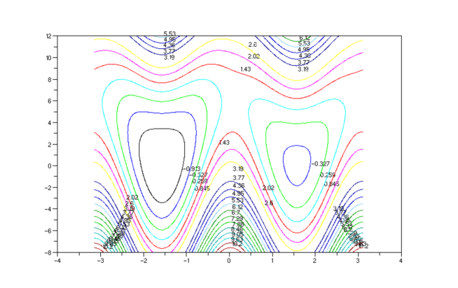
Figure 2: Contour plot of the potential $V$.

The dynamics is discretized using an Euler-Maruyama scheme with timestep $\delta t=10^{-4}$ over the time interval $[0,10^{4}]$. We use a mesh of $(-\pi,\pi]$ with $I=40$ intervals of the same size. The function $x\mapsto\Psi_{t}(x)$ is approximated over this mesh using continuous piecewise affine interpolation. The width of the Gaussians is set to the size of the intervals: $\varepsilon=2\pi/I$.

In the following, we compare, for $x\in\mathbb{T}$, $-F^{\prime}(x)$ with $\lim_{t\to\infty}\frac{1}{t}\int_{0}^{t}\frac{d\Psi_{s}}{dx}(x)\,ds$. We have checked numerically that the longtime limit is attained at $t=10^{4}$.

We observe on Figures 3, 4 and 5 that the quality of the result highly depends on the choice of the parameter $\gamma$: as $\gamma$ decreases, the result gets closer to the expected answer. This justifies the use of a parameter $\gamma$ depending on time $t$ and going to zero in the longtime limit (vanishing adaption), as in Wang Landau [WL01], in Well Tempered Metadynamics [BBP08] or in Self Healing Umbrella Sampling [Mar+06].

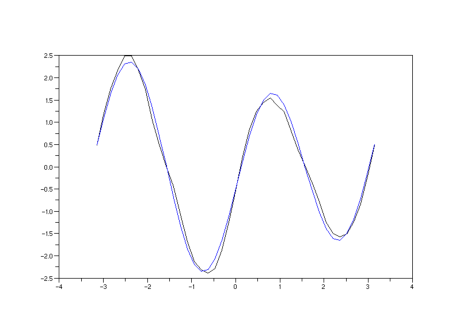
Figure 3: Comparison of the mean force profiles, $\gamma=0.1$. Blue: $-F^{\prime}(x)$. Black: $\lim_{t\to\infty}\frac{1}{t}\int_{0}^{t}\frac{d\Psi_{s}}{dx}(x)\,ds$.

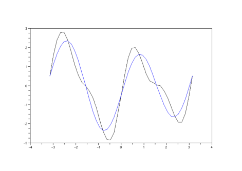
Figure 4: Comparison of the mean force profiles, $\gamma=1$. Blue: $-F^{\prime}(x)$. Black: $\lim_{t\to\infty}\frac{1}{t}\int_{0}^{t}\frac{d\Psi_{s}}{dx}(x)\,ds$.

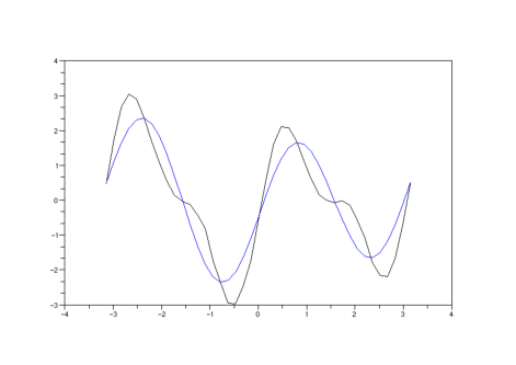
Figure 5: Comparison of the mean force profiles, $\gamma=10$. Blue: $-F^{\prime}(x)$. Black: $\lim_{t\to\infty}\frac{1}{t}\int_{0}^{t}\frac{d\Psi_{s}}{dx}(x)\,ds$.

2.2 Discrete state space metadynamics: an analytical study

2.2.1 The non-adiabatic metadynamics

The non-adiabatic version of the discrete metadynamics introduced in Section 1.2 consists in grouping states into a certain number of bins, and compute the bias not site by site, but bin by bin. More precisely let $\xi:\{0,\ldots,K\}\to\{0,\ldots,B\}$ be a collective variable, with $B<K$: the bins are the levet sets $(\xi^{-1}(\{b\}))_{0\leq b\leq B}$. Let us record the current position of the walker $I_{t}\in\{0,\ldots,K\}$ and the local times spent in each bin $b\in\{0,\ldots,B\}$

$$L_{t}(b)=\int_{0}^{t}\mathbf{1}_{\xi(I_{s})=b}ds$$

so that $L_{t}=(L_{t}(0),\ldots,L_{t}(B))\in\mathbb{R}^{B+1}$. Let $V:\{0,\ldots,K\}\to\mathbb{R}$ be the potential function and let us define

$$\forall k\in\{1,\ldots,K\},V_{k}^{\prime}=V_{k}-V_{k-1}.$$

The generator of the process $(L_{t},I_{t})_{t\geq 0}$ is given by: for any test function $f:\mathbb{R}^{B+1}\times\{0,\ldots,K\}\to\mathbb{R}$, for all $(l,k)\in\mathbb{R}^{B+1}\times\{0,\ldots,K\}$,

$$\begin{split}Lf(l,k)=&\partial_{l_{k}}f(l,k)\\ &+1_{\{k<K\}}\exp\left(-\beta(\gamma[l(\xi(k+1))-l(\xi(k))]+V^{\prime}_{k+1})\right)\left(f(l,k+1)-f(l,k)\right)\\ &+1_{\{k>0\}}\exp\left(+\beta(\gamma[l(\xi(k))-l(\xi(k-1))]+V^{\prime}_{k})\right)\left(f(l,k-1)-f(l,k)\right).\end{split}$$

Just as in Section 1.2, we could instead define a process acting on the differences of local times — since the expression of the generator is messier we omit it.

One could hope that this process, similarly to the simpler one we described in the Section 1.2, ”learns the free energy profile”, in the sense that the difference of local times $\gamma(L_{t}(b)-L_{t}(b^{\prime}))$ (for $(b,b^{\prime})\in\{0,\ldots,B\}^{2}$) fluctuates around the difference of free energy

$$A_{b^{\prime}}-A_{b}=\frac{1}{2\beta}\ln{{\left(\frac{\pi(\xi^{-1}(\{b\}))}{\pi(\xi^{-1}(\{b^{\prime}\}))}\right)}}$$

where for $k\in\{0,\ldots,K\}$, $\pi(\{k\})=\frac{e^{-2\beta V_{k}}}{\sum_{j=0}^{K}e^{-2\beta V_{j}}}$. Should this hold, then the free energy profile $(A_{b})_{0\leq b\leq B}$ could then be recovered by taking time averages.

Unfortunately this is not the case. To see why, we consider a simple case with $4$ sites $\{0,1,2,3\}$ and two bins: $B_{-}=\{0,1\}$ and $B_{+}=\{2,3\}$. We define the potential $V$ by $V_{1}=V_{2}$, $V_{1}-V_{0}=D_{-}>0$ and $V_{2}-V_{3}=D_{+}>0$: $V$ has two wells in $0$ and $3$, separated by a saddle $\{1,2\}$. We let

$$\lambda_{\pm}=\exp(-\beta D_{\pm})$$

be the jump rates from the bottom of the wells to the saddle.

The target measure is proportional to $\exp(-2\beta V)$; the weights it gives to each bin are

$$\pi(B_{-})= \frac{1+\lambda_{-}^{-2}}{2+\lambda_{-}^{-2}+\lambda_{+}^{-2}} \pi(B_{+})= \frac{1+\lambda_{+}^{-2}}{2+\lambda_{-}^{-2}+\lambda_{+}^{-2}}$$

so the difference of local times $X_{t}=\gamma(L_{t}(+)-L_{t}(-))$ should fluctuate around

$$A_{-}-A_{+}=\frac{1}{2\beta}\ln{{\left(\frac{1+\lambda_{+}^{-2}}{1+\lambda_{-}^{-2}}\right)}}.$$ (27)

For this model however, the heuristic picture is very different:

the trajectorial average of $$(X_{t}) \gamma\left(\frac{1}{\lambda_{+}}-\frac{1}{\lambda_{-}}\right)$$ behaves like , (28)

at least when $\gamma$ is sufficiently large, and this limit is indeed different from the free energy difference (27). We justify this claim with an informal reasoning just below, and with an analytical proof in a slightly simplified setting in Section 2.2.2.

Let us first give an idea of the trajectories of the process in the large $\gamma$ regime. Starting from $i=0$ and $x=0$, the process:

1. stays in $0$ for a time $E_{-}$ (exponential with parameter $\lambda_{-}$),

2. jumps to $1$, where it immediately jumps to $2$ (since at that time, $X_{t}=-\gamma E_{-}$, with $\gamma E_{-}$ very large), and then quickly jumps to $3$.

At this point $|X_{t}|$ is large. While it stays large, even if $I_{t}$ jumps to $2$ it will quickly jump back to $3$, since the jump to $1$ is essentially blocked. So the process must wait in $3$ for a time at least $E_{-}$, so that $X_{t}$ has time to decrease back to $0$. After this, the process waits for an exponential time $E_{+}$ (with parameter $\lambda_{+}$) until it jumps to $2$. Once more it jumps immediately to $1$ and then to $0$, and must stay there (with brief visits to $1$) until $X_{t}$ comes back to $0$. During such a cycle, of duration $T=2(E_{-}+E_{+})$, $\int_{0}^{T}X_{s}ds$ is approximately $-\gamma E_{-}^{2}+\gamma E_{+}^{2}$. In expectation this yields $(2\gamma)(\lambda_{+}^{-2}-\lambda_{-}^{-2})$. By the ergodic theorem, since $\mathbb{E}\left[T\right]=2(\lambda_{+}^{-1}+\lambda_{-}^{-1})$, this gives the claimed approximation (28): $\frac{1}{t}\int_{0}^{t}X_{s}\,ds\approx_{t\to\infty}\gamma\left(\frac{1}{\lambda_{+}}-\frac{1}{\lambda_{-}}\right)$.

We tested this claim numerically for various values of $\gamma$, $\lambda_{\pm}$, see Figure 6 for an illustration.

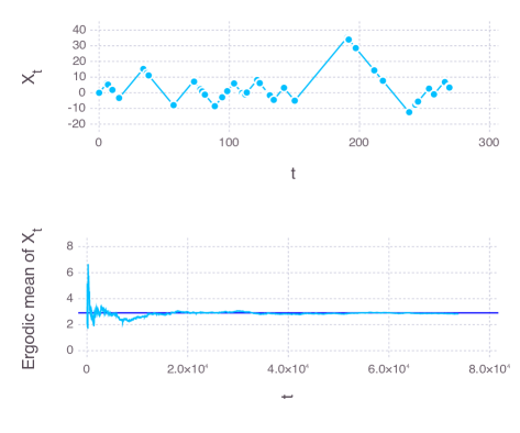
An example trajectory for the four-states, two bins model, in the uneven double well potential $V$ given by $V_{0}=0$, $V_{1}=V_{2}=2$ and $V_{3}=0.5$, with $\gamma=1$ and $\beta=1$. Upper plot: the trajectory of $X_{t}$. The dots represent times when $I_{t}$ jumps. Lower plot: the ergodic mean $\frac{1}{t}\int_{0}^{t}X_{s}ds$. The horizontal line is $\gamma\left(\frac{1}{\lambda_{+}}-\frac{1}{\lambda_{-}}\right)$.

Figure 6: The four-states, two-bins model.

Rather than trying to make this informal picture more precise, we simplify the model a bit more in the next section so that it becomes analytically tractable.

2.2.2 Analytical results on a simplified non-adiabatic metadynamics

In order to be able to write an explicit expression for the invariant measure, we modify the model with 4 sites and 2 bins considered in the previous section. We idealize the saddle $\{1,2\}$ and replace it by an abstract state; we relabel the states to $\{-,0,+\}$ where $-$ and $+$ are the two wells and $0$ is the saddle between them. Let us then define the following generator:

$$L^{simp}f(x,i) =\gamma i\partial_{x}f(x,i)+1_{\{i=\pm\}}\lambda_{\pm}(f(x,0)-f(x,\pm))$$ (29)

$$\quad+1_{\{i=0\}}\left(\frac{e^{\beta x}}{\lambda_{-}}(f(x,-)-f(x,0))+\frac{e^{-\beta x}}{\lambda_{+}}(f(x,+)-f(x,0))\right).$$

The measure

$$d\mu^{simp}(x,i)=\delta_{-}(di)\mu_{-}(x)dx+\delta_{0}(di)\mu_{0}(x)dx+\delta_{+}(di)\mu_{+}(x)dx$$ (30)

is invariant for the dynamics with generator $L^{simp}$ if and only if

$$\left\{\begin{aligned} \gamma\mu_{-}^{\prime}(x)-\lambda_{-}\mu_{-}(x)+\frac{e^{\beta x}}{\lambda_{-}}\mu_{0}(x)=&0\\ \lambda_{-}\mu_{-}(x)+\lambda_{+}\mu_{+}(x)-\left(\frac{e^{\beta x}}{\lambda_{-}}+\frac{e^{-\beta x}}{\lambda_{+}}\right)\mu_{0}(x)=&0\\ \gamma\mu_{+}^{\prime}(x)+\lambda_{+}\mu_{+}(x)-\frac{e^{-\beta x}}{\lambda_{+}}\mu_{0}(x)=&0.\end{aligned}\right.$$

This system is equivalent to

$$\left\{\begin{aligned} \mu_{0}(x)=&\frac{\lambda_{+}\lambda_{-}^{2}\mu_{-}(x)+\lambda^{2}_{+}\lambda_{-}\mu_{+}(x)}{\lambda_{+}e^{\beta x}+\lambda_{-}e^{-\beta x}}\\ \gamma\mu_{-}^{\prime}(x)=\gamma\mu_{+}^{\prime}(x)=&\frac{\lambda_{-}^{2}e^{-\beta x}\mu_{-}(x)-\lambda_{+}^{2}e^{\beta x}\mu_{+}(x)}{\lambda_{+}e^{\beta x}+\lambda_{-}e^{-\beta x}}.\end{aligned}\right.$$

The last equation implies that $\mu_{-}(x)-\mu_{+}(x)$ is constant and for the invariant measure to be finite that $\mu_{-}(x)=\mu_{+}(x)$. Hence

$$\left\{\begin{aligned} \mu_{-}(x)=&\mu_{+}(x)\\ \mu_{0}(x)=&\frac{\lambda_{+}\lambda_{-}^{2}+\lambda^{2}_{+}\lambda_{-}}{\lambda_{+}e^{\beta x}+\lambda_{-}e^{-\beta x}}\mu_{+}(x)\\ \gamma\mu_{+}^{\prime}(x)=&\frac{\lambda_{-}^{2}e^{-\beta x}-\lambda_{+}^{2}e^{\beta x}}{\lambda_{+}e^{\beta x}+\lambda_{-}e^{-\beta x}}\mu_{+}(x).\end{aligned}\right.$$

Setting $\tilde{\mu}(y)=\mu_{+}\left(\frac{\ln(y)}{\beta}\right)$, one has

$$(\ln\tilde{\mu})^{\prime}(y)=\frac{1}{\gamma\beta}\frac{\lambda_{-}^{2}-\lambda_{+}^{2}y^{2}}{\lambda_{+}y^{3}+\lambda_{-}y}=\frac{1}{\gamma\beta}\left(\frac{\lambda_{-}}{y}-\frac{\lambda_{+}(\lambda_{+}+\lambda_{-})y}{\lambda_{+}y^{2}+\lambda_{-}}\right).$$

One concludes that

$$\mu_{+}(x)=\frac{1}{C}e^{\frac{\lambda_{-}}{\gamma}x}(\lambda_{+}e^{2\beta x}+\lambda_{-})^{-\frac{\lambda_{+}+\lambda_{-}}{2\beta\gamma}}=\frac{1}{C}\left(\lambda_{+}e^{\frac{2\beta\lambda_{+}}{\lambda_{+}+\lambda_{-}}x}+\lambda_{-}e^{-\frac{2\beta\lambda_{-}}{\lambda_{+}+\lambda_{-}}x}\right)^{-\frac{\lambda_{+}+\lambda_{-}}{2\beta\gamma}}$$ (31)

where the constant $C$ is chosen so that $\mu$ is a probability measure. To simplify notation define $x_{0}=\frac{1}{2\beta}\ln(\lambda_{-}/\lambda_{+})=\frac{1}{2}\left(D_{+}-D_{-}\right)$, $d=\lambda_{+}-\lambda_{-}$ and $s=\lambda_{+}+\lambda_{-}$. Then

$$\lambda_{+}\exp{{\left(\frac{2\beta\lambda_{+}x}{\lambda_{+}+\lambda_{-}}\right)}}+\lambda_{-}\exp{{\left(\frac{-2\beta\lambda_{-}x}{\lambda_{+}+\lambda_{-}}\right)}}=\exp{{\left(\frac{\beta dx}{s}\right)}}2\cosh(\beta(x-x_{0}))\sqrt{\lambda_{-}\lambda_{+}}$$

The density of the marginal of the invariant measure $\mu^{simp}$ on the $x$ variable is proportional to:

$$f(x)=\exp{{\left(-\frac{d(x-x_{0})}{2\gamma}\right)}}(2\cosh(\beta(x-x_{0})))^{-s/(2\beta\gamma)}{{\left(2+\frac{s\sqrt{\lambda_{-}\lambda_{+}}}{2\cosh(\beta(x-x_{0}))}\right)}}.$$

Lemma 2.1 (Asymptotics for $\int xd\mu^{simp}(x,i)$).

Assume that $D_{+}\neq D_{-}$. Then, the average of $x$ under the invariant measure $d\mu^{simp}(x,i)$ defined by (30)–(31) behaves like $\gamma{{\left(e^{\beta D_{+}}-e^{\beta D_{-}}\right)}}$ when this quantity is large in absolute value, in the sense that

$$\frac{1}{\gamma{{\left(e^{\beta D_{+}}-e^{\beta D_{-}}\right)}}}\int xd\mu^{simp}(x,i)\to 1,$$

when any one of the parameters $\beta$, $\gamma$, $D_{+}$ or $D_{-}$ goes to infinity while the others stay fixed.

Remark 7.

In the symmetric case $D_{-}=D_{+}$, the mean value of $x$ is zero.

Proof.

We wish to compute the limit of $\displaystyle m(\beta,\gamma,D_{+},D_{-})=\frac{\int xf(x)dx}{\int f(x)dx}$ when one of the parameters $\beta$, $\gamma$, $D_{+}$ or $D_{-}$ goes to infinity. We change variables by setting $x=x_{0}+\gamma{{\left(\frac{1}{\lambda_{+}}-\frac{1}{\lambda_{-}}\right)}}y=x_{0}-\frac{\gamma d}{\lambda_{-}\lambda_{+}}y$. Let $g(y)=f{{\left(x_{0}-\frac{\gamma d}{\lambda_{-}\lambda_{+}}y\right)}}$. Then

$$m(\beta,\gamma,D_{-},D_{+})=x_{0}-\frac{\gamma d}{\lambda_{-}\lambda_{+}}\frac{\int yg(y)dy}{\int g(y)dy},$$

where

$$g(y)=\exp{{\left(\frac{d^{2}}{2\lambda_{-}\lambda_{+}}y\right)}}{{\left(2\cosh{{\left(\frac{\beta\gamma d}{\lambda_{-}\lambda_{+}}y\right)}}\right)}}^{-s/(2\beta\gamma)}{{\left(2+\frac{s\sqrt{\lambda_{-}\lambda_{+}}}{2\cosh{{\left(\frac{\beta\gamma d}{\lambda_{-}\lambda_{+}}y\right)}}}\right)}}.$$

We thus have, since $\gamma(e^{\beta D_{-}}-e^{\beta D_{+}})=\frac{\gamma d}{\lambda_{-}\lambda_{+}}$:

$$\frac{1}{\gamma{{\left(e^{\beta D_{+}}-e^{\beta D_{-}}\right)}}}m(\beta,\gamma,D_{-},D_{+})=\frac{D_{+}-D_{-}}{2\gamma{{\left(e^{\beta D_{+}}-e^{\beta D_{-}}\right)}}}+\frac{\int yg(y)dy}{\int g(y)dy}.$$

For any of the limits we consider, the first term in the right-hand side goes to zero, and for any fixed $y$, $\frac{\gamma d}{\lambda_{-}\lambda_{+}}$ goes to infinity so that

$$g(y) \sim 2\exp{{\left(\frac{d^{2}}{2\lambda_{-}\lambda_{+}}y\right)}}{{\left(\exp{{\left(-\frac{s{{\left|d\right|}}}{2\lambda_{-}\lambda_{+}}{{\left|y\right|}}\right)}}\right)}}$$

$$\sim\begin{cases}2\exp{{\left(-\frac{{{\left|d\right|}}}{\max(\lambda_{-},\lambda_{+})}{{\left|y\right|}}\right)}},&\text{ if }y>0\\ 2\exp{{\left(-\frac{{{\left|d\right|}}}{\min(\lambda_{-},\lambda_{+})}{{\left|y\right|}}\right)}},&\text{ if }y<0.\end{cases}$$

Let us write $h(y)$ for the last function appearing in these equivalences.

Consider first the $\gamma\to\infty$ limit. The function $h(y)$ does not depend on $\gamma$, and a direct computation shows that:

$$\int yh(y)dy= \frac{2}{{{\left|d\right|}}^{2}}{{\left(\max(\lambda_{-},\lambda_{+})^{2}-\min(\lambda_{-},\lambda_{+})^{2}\right)}}$$

$$= \frac{2}{{{\left|d\right|}}}{{\left(\max(\lambda_{-},\lambda_{+})+\min(\lambda_{-},\lambda_{+})\right)}}=\int h(y)dy.$$

Since $yg(y)$ is easy to dominate, we get by Lebesgue’s theorem:

$$\frac{1}{\gamma{{\left(e^{\beta D_{+}}-e^{\beta D_{-}}\right)}}}m(\beta,\gamma,D_{-},D_{+})\to\frac{\int yh(y)dy}{\int h(y)dy}=1.$$

For the other cases, where one of $\beta$, $D_{-}$ or $D_{+}$ converges to $\infty$ with all other parameters fixed, we compute one step further to get

$$g(y)\sim h(y)\to 2\mathbf{1}_{y>0}\exp{{\left(-y\right)}}.$$

We apply Lebesgue’s theorem once more: $\int yg(y)dy/\int g(y)dy$ converges to $\int_{0}^{\infty}ye^{-y}dy/\int_{0}^{\infty}e^{-y}dy=1$, and the result follows. ∎

The fact that the trajectorial average of $X_{t}$ converges to $\int xd\mu^{simp}(x,i)$ is guaranteed by the following result.

Lemma 2.2.

The process $(X_{t},I_{t})$ with generator $L^{simp}$ defined by (29) is exponentially ergodic (in the sense of Equation (18)) with respect to the measure $\mu^{simp}$ defined by (30)–(31). Furthermore we have the convergence of the ergodic mean:

$$\frac{1}{t}\int_{0}^{t}X_{s}ds\xrightarrow{\text{a.s.}}\int xd\mu^{simp}(x,i).$$

Proof.

We build a function $W$ that satisfies

$$L^{simp}W(x,i)\leq-\delta W(x,i)+M\mathbf{1}_{{{\left|x\right|}}\leq C}.$$

If the process starts in $\{-,0,+\}\times[C,\infty)$, it cannot reach $\{-,0,+\}\times(-\infty,-C]$ without coming back in the compact $\{-,0,+\}\times[-C,C]$. Therefore we may define $W$ separately on $\{-,0,+\}\times\mathbb{R}_{+}$ and $\{-,0,+\}\times\mathbb{R}_{-}$. We only do the first case, the second being similar. On $\mathbb{R}_{+}\times\{-,0,+\}$, let $W(x,i)=C_{i}e^{\alpha x}$ where the constants satisfy $0<C_{-}<C_{0}<C_{+}$ and

$$\lambda_{-}\left(\frac{C_{0}}{C_{-}}-1\right)<\gamma\alpha<\lambda_{+}{{\left(1-\frac{C_{0}}{C_{+}}\right)}}.$$

Such a choice is always possible by choosing $C_{0}=1$, $C_{+}=2$ and $C_{-}$ close enough to $1$. A simple computation yields

$$L^{simp}W(x,+)= \gamma\alpha C_{+}e^{\alpha x}+\lambda_{+}(C_{0}e^{\alpha x}-C_{+}e^{\alpha x})$$

$$= -{{\left(\lambda_{+}{{\left(1-\frac{C_{0}}{C_{+}}\right)}}-\gamma\alpha\right)}}W(x,+),$$

$$L^{simp}W(x,0)= \frac{e^{\beta x}}{\lambda_{-}}(C_{-}-C_{0})e^{\alpha x}+\frac{e^{-\beta x}}{\lambda_{+}}(C_{+}-C_{0})e^{\alpha x}$$

$$= -{{\left(\frac{e^{\beta x}}{\lambda_{-}}{{\left(1-\frac{C_{-}}{C_{0}}\right)}}-\frac{e^{-\beta x}}{\lambda_{+}}{{\left(\frac{C_{+}}{C_{0}}-1\right)}}\right)}}W(x,0)$$

$$L^{simp}W(x,-)= -\gamma\alpha C_{-}e^{\alpha x}+\lambda_{-}{{\left(C_{0}e^{\alpha x}-C_{-}e^{\alpha x}\right)}}$$

$$= -{{\left(\gamma\alpha-\lambda_{-}{{\left(\frac{C_{0}}{C_{-}}-1\right)}}\right)}}W(x,-)$$

so that $L^{simp}W\leq-\delta W+C\mathbf{1}_{{{\left|x\right|}}\leq C}$ for appropriate choices of $C<\infty$ and $\delta>0$.

The exponential ergodicity follows by classical arguments that will be developed below in the proof of Theorem 3.6: the process is irreducible, aperiodic and the compact set $\{-,0,+\}\times[-C,C]$ is petite, so the ergodicity follow from [DMT95, Theorem 5.2 (c)].

The fact that the ergodic mean converges then follows from the fact that $(x,i)\mapsto x$ is locally bounded, so that Equation (20) holds, and we can follow the same proof as for Theorem 1.6. ∎

3 Mathematical analysis of the adiabatic discrete case

We prove the main mathematical results, Theorems 1.5, 1.6 and 1.7, as follows. We start in Section 3.1 by checking the explicit expression of the invariant measure. In Section 3.2, we state that there exists an explicit Lyapunov function $W$ such that, for “nice” starting points $(x,i)$, $P_{t}W(x,i)\leq\kappa W(x,i)$ (where $P_{t}$ is the transition operator associated with the infinitesimal generator (17)). This is the content of Theorem 3.3, the proof of which is postponed to Section 3.6 for ease of reading. Using this, we prove in Section 3.3 that $W$ is a Lyapunov function for an auxiliary, discrete time Markov chain, from which we deduce the control on return times stated in Theorem 1.9. We proceed to the proof of the main results, Theorems 1.5, 1.6 and 1.7, in Section 3.4. Finally, we establish in Section 3.5 precise bounds for the process appearing in the Ray-Knight representation already stated in Section 1.2.3; in turn, these bounds enable us to prove the key intermediate result Theorem 3.3 in Section 3.6.

3.1 The invariant measure

We prove here the explicit expression of the invariant measure announced in Proposition 1.3. Let $f:\mathbb{R}^{K}\times\{0,\ldots,K\}\to\mathbb{R}$ be a nice function (say, for each $k\in\{0,\ldots,K\}$, $x\mapsto f(x,k)$ is smooth with compact support) and let us compute $\int Lfd\mu$.

$$Z\times\int Lf(x,k)d\mu(x,k)= \gamma\int\sum_{0<k\leq K}\partial_{k}f(x,k)\exp(-\sum_{j}g_{j}(x_{j}))dx_{1}\cdots dx_{K}$$

$$\quad-\gamma\int\sum_{0\leq k<K}\partial_{k+1}f(x,k)\exp(-\sum_{j}g_{j}(x_{j}))dx_{1}\cdots dx_{K}$$

$$\quad+\int\sum_{0\leq k<K}e^{-\beta(x_{k+1}+A^{\prime}_{k+1})}f(x,k+1)dm(x)-\int\sum_{0\leq k<K}e^{-\beta(x_{k+1}+A^{\prime}_{k+1})}f(x,k)dm(x)$$

$$\quad+\int\sum_{0<k\leq K}e^{\beta(x_{k}+A^{\prime}_{k})}f(x,k-1)dm(x)-\int\sum_{0<k\leq K}e^{\beta(x_{k}+A^{\prime}_{k})}f(x,k)dm(x).$$

In the first two terms, we swap the sum and integral signs and integrate by parts, respectively on the $x_{k}$ and $x_{k+1}$ variables. In the third and fifth term we shift indices to get:

$$Z\times\int Lf(x,k)d\mu(x,k) =\gamma\int\sum_{0<k\leq K}f(x,k)g_{k}^{\prime}(x_{k})dm(x)-\gamma\int\sum_{0\leq k<K}f(x,k)g_{k+1}^{\prime}(x_{k+1})dm(x)$$

$$\quad+\int\sum_{0<k\leq K}e^{-\beta(x_{k}+A^{\prime}_{k})}f(x,k)dm(x)-\int\sum_{0\leq k<K}e^{-\beta(x_{k+1}+A^{\prime}_{k+1})}f(x,k)dm(x)$$

$$\quad+\int\sum_{0\leq k<K}e^{\beta(x_{k+1}+A^{\prime}_{k+1})}f(x,k)dm(x)-\int\sum_{0<k\leq K}e^{\beta(x_{k}+A^{\prime}_{k})}f(x,k)dm(x)$$

$$=\int\sum_{0<k\leq K}f(x,k){{\left(\gamma g_{k}^{\prime}(x_{k})+e^{-\beta(x_{k}+A^{\prime}_{k})}-e^{\beta(x_{k}+A^{\prime}_{k})}\right)}}dm(x)$$

$$\quad+\int\sum_{0\leq k<K}f(x,k){{\left(-\gamma g_{k+1}^{\prime}(x_{k+1})-e^{-\beta(x_{k+1}+A^{\prime}_{k+1})}+e^{\beta(x_{k+1}+A^{\prime}_{k+1})}\right)}}dm(x)$$

by regrouping terms in the sums. Since $\gamma g^{\prime}_{k}(y)=e^{\beta(y+A^{\prime}_{k})}-e^{-\beta(y+A^{\prime}_{k})}$, the terms between brackets vanish, so $\int Lf(x,k)d\mu(x,k)=0$ and $\mu$ is invariant.

3.2 Bounds for $t$-separated starting points

Definition 3.1 (Separated configuration and plateau).

Let $A>a>0$ and $t>0$.

• A configuration $(x,i)\in\mathbb{R}^{K}\times\{0,\ldots,K\}$ (or a vector $x\in\mathbb{R}^{K}$) is called $(t,a,A)$-separated if the components of $x$ are either very large or very small, in the sense that

  $$\forall j\in\{1,\ldots,K\},\quad{{\left|x_{j}\right|}}\leq at\text{ or }{{\left|x_{j}\right|}}>At,$$

  and at least one of the $|x_{j}|$ is larger than $At$.

• A connected set of sites $I=\{l,l+1,\ldots,r-1\}\subset\{0,\ldots,K\}$ (for $l\leq r-1$) is called a plateau of a $(t,a,A)$-separated vector $x\in\mathbb{R}^{K}$ if

  • ${{\left|x_{j}\right|}}<at$ for all $l<j<r$,

  • when $l\geq 1$, $x_{l}>At$,

  • when $r\leq K$, $x_{r}<-At$.

For a vecteur $x\in\mathbb{R}^{K}$, let us consider, for $k\in\{0,\ldots,K\}$, $l_{k}=\sum_{m=1}^{k}x_{m}$: a plateau is a connected set of sites where $l$ does not vary too much, with on the boundaries of the plateau a drop to lower values. In the following, we will refer to sites which are not on a plateau as wells. We refer to Figure 7 for a schematic representation of a separated vector, with its plateaux.

Lemma 3.2.

Any $(t,a,A)$-separated vector $x\in\mathbb{R}^{K}$ admits a plateau.

Proof.

We proceed by induction on $K$. If $K=1$, then either $x_{1}<-At$ and $I=\{0\}$ is a plateau or $x_{1}>At$ and $I=\{1\}$ is a plateau. Let us assume that the result holds when $1\leq K<\bar{K}$ with $\bar{K}\geq 2$ and let $(x,i)\in\mathbb{R}^{\bar{K}}\times\{0,\ldots,\bar{K}\}$ be $(t,a,A)$-separated. Let $\underline{j}=\min\{j\geq 1:|x_{j}|>At\}$. If $x_{\underline{j}}<-At$, then $I=\{0,\ldots,\underline{j}-1\}$ is a plateau. If $x_{\underline{j}}>At$, then either $\max_{\underline{j}+1\leq j\leq\bar{K}}|x_{j}|\leq at$ and $I=\{\underline{j},\ldots,\bar{K}\}$ is a plateau or $\max_{\underline{j}+1\leq j\leq\bar{K}}|x_{j}|>At$. In the latter case, $(x_{\underline{j}+1},\ldots,x_{\bar{K}})$ is $(t,A,a)$-separated and admits a plateau by the induction hypothesis at rank $\bar{K}-\underline{j}<\bar{K}$. The translation by $\underline{j}$ of the indices of this plateau form a plateau of $(x_{0},\ldots,x_{K})$ since $x_{\underline{j}}>At$. ∎

Starting from a $(t,a,A)$-separated configuration $(x,i)$, the process with generator (17) is highly predictable on the $t$ time scale: if $a$ is small enough and $A$ large enough, then during a time $t$, the process will (almost always) either jump to to lower energy sites or jump over small barriers of size $at$ but (almost never) over large barriers of size $At$. This is because over the time $t$, the process cannot fill the wells of the initial configuration. Let us state this fact more precisely. For a configuration $x$, let

$$(l_{0},\ldots,l_{K})=(l_{0},l_{0}+x_{1},x_{1}+x_{2},\ldots,l_{0}+x_{1}+\ldots+x_{K})$$ (32)

be a discrete antiderivative of $x$ (where $l_{0}$ is completely arbitrary and plays no role in the dynamics and in the value of $S(x)$) and let us recall the definition of the function $S$ introduced in (19), written here in terms of the antiderivative $l$:

$$S(x)=\sum_{i=0}^{K}\left(\left(\max_{0\leq j\leq K}l_{j}\right)-l_{i}\right).$$ (33)

This represents the amount of ”computational sand” needed to fill all the gaps in $x$ (see Figure 7). Notice that

$$S(x)\leq K\sum_{k=1}^{K}|x_{k}|.$$ (34)

On both pictures the blue bars represent the profile $l_{0},l_{1},...,l_{K}$, that satisfies $x_{k}=l_{k}-l_{k-1}$. The value of $l_{0}$ can be chosen arbitrarily (energy landscapes are defined up to an additive constant). On the left: a separated configuration with two plateaus: $\{0,1,2\}$ and $\{4,5\}$ (for $(t,a,A)=(1,1/2,3/2)$, see Defintion 3.1). On the right: The function $S(x)$ is the sum of the lengths in red (see (19)).

Figure 7: Schematic representation of the plateaus of a separated vector, and of the function $S$.

Starting from a $(t,a,A)$-separated configuration $(x,i)$, then between time $0$ and $t$, the process $(I_{t})_{t\geq 0}$ will behave essentially essentially as follows: if $i$ is in a well, $I_{t}$ will stay in this well, if $i$ is on a plateau, $I_{t}$ will go very quickly in one of the wells on the boundaries of the plateau, and stay there. In both cases, the process $I_{t}$ will stay for a long time in a well and “fill it up”, until time $t$: this will thus decrease the values of $S(X_{t})$. This is quantified in the following theorem, and it yields a natural Lyapunov function for the process $(X_{t},I_{t})$.

Theorem 3.3.

Let us consider the process $(X_{t},I_{t})$ with generator (17). Let us denote by $P_{t}$ the associated transition operator, and $(x,i)$ the initial condition of the process. There exist positive numbers $a<A$, $\chi$, $t_{0}$ and $\kappa\in(0,1)$, such that for all $t\geq t_{0}$, for all starting points $(x,i)\in\mathbb{R}^{K}\times\{0,\ldots,K\}$,

$$(x,i)\text{ is }(t,a,A)\text{-separated}\implies P_{t}W(x,i)\leq\kappa W(x,i)$$

where $W(x,i)=\exp(\chi S(x))$.

The proof of this theorem is given below in Section 3.6. It draws on the Ray-Knight description of the process found in [TV11] and already introduced in Section 1.2.3.

3.3 Exponential moments for return times — Theorem 1.9

Let $t_{0}$, $a$, $A$ be given by Theorem 3.3. For $k\in\{0,\ldots,K\}$, let $t_{k}=t_{0}(A/a)^{k}$, and let

$$\forall k\in\{0,\ldots,K-1\},\,\mathcal{S}_{k}=\left\{x\in\mathbb{R}^{K},x\text{ is $(t_{k},a,A)$-separated}\right\}.$$

Finally let us introduce the compact set $\mathcal{K}\subset\mathbb{R}^{K}$:

$$\mathcal{K}=\left\{x\in\mathbb{R}^{K},\,\max{{\left|x_{j}\right|}}\leq At_{K-1}\right\}.$$

One has $\mathbb{R}^{K}={{\left(\bigcup_{k=0}^{K-1}\mathcal{S}_{k}\right)}}\cup\mathcal{K}$. Indeed, if $x$ is not in $\mathcal{K}$, then one of its $K$ coordinates is larger in absolute value than $At_{K-1}$ and since the $K$ intervals $]at_{0},At_{0}]$, $]at_{1},At_{1}]$,…, $]at_{K-1},At_{K-1}]$ are disjoint, there is an index $k\in\{0,\ldots,K-1\}$ such that $]at_{k},At_{k}]$ contains no coordinate of $x$ so that $x\in\mathcal{S}_{k}$.

Define the discrete time Markov chain $(Y_{n},J_{n})_{n\in\mathbb{N}}$ with values in $\mathbb{R}^{K}\times\{0,\ldots,K\}$ as follows: at step $n$, from $(Y_{n},J_{n})=(y,j)$, compute $\underline{k}(y)=\min\{k\in\{0,\ldots,K-1\}:y\in\mathcal{S}_{k}\}$ with convention $\min\emptyset=K$ (applied when $y\in\mathcal{K}\setminus\bigcup_{k=0}^{K-1}\mathcal{S}_{k}$), run the continuous time process $(X_{t},I_{t})_{t\geq 0}$ with generator (17) starting from $(X_{0},I_{0})=(y,j)$ for a time $t_{\underline{k}(y)}$ and then set $(Y_{n+1},J_{n+1})=(X_{t_{\underline{k}(y)}},I_{t_{\underline{k}(y)}})$. Notice that for any $y\in\mathbb{R}^{K}$, $t_{\underline{k}(y)}\in\{t_{0},t_{1},\ldots,t_{K}\}$. Let us denote by $P$ the transition operator for $(Y_{n},J_{n})_{n\in\mathbb{N}}$.

Lemma 3.4.

The function $W$ defined in Theorem 3.3 is a Lyapunov function for the chain $(Y_{n},J_{n})$: there exist two constants $C<\infty$ and $\kappa<1$ such that, for all $(y,j)\in\mathbb{R}^{K}\times\{0,\ldots K\}$

$$PW(y,j)\leq\kappa W(y,j)+C\mathbf{1}_{\mathcal{K}}(y,j).$$ (35)

Moreover, the return time to $\mathcal{K}$ has exponential moments: there exists $\tilde{\delta}>0$ and $\tilde{C}<\infty$ such that, for all $(y,j)\in\mathbb{R}^{K}\times\{0,\ldots K\}$

$$\mathbb{E}_{(y,j)}\left[e^{\tilde{\delta}\tilde{\tau}_{\mathcal{K}}}\right]\leq\tilde{C}W(y,j)$$ (36)

where $\tilde{\tau}_{\mathcal{K}}=\inf\{n\geq 1:\,Y_{n}\in\mathcal{K}\}$ is the first entry time in $\mathcal{K}\times\{0,\ldots,K\}$ for the chain $(Y_{n},J_{n})$.

Proof.

The fact that (35) holds when $y\in\bigcup_{k=0}^{K-1}\mathcal{S}_{k}$ is a straightforward consequence of Theorem 3.3 and the definition of the chain $(Y_{n},J_{n})$. Otherwise, when $y\in\mathcal{K}\setminus\bigcup_{k=0}^{K-1}\mathcal{S}_{k}$, for all $k\in\{1,\ldots,K\}$, $|Y_{1}(k)|\leq|y_{k}|+t_{K}\leq At_{K-1}+t_{K}$, so that, by (34), $W(Y_{1},J_{1})\leq e^{K^{2}(At_{K-1}+t_{K})}$ and (35) still holds, by choosing appropriately $C$.

To bound the return times, we apply [MT09, Theorem 15.3.3] which states that the drift condition (35) and the fact that $\mathcal{K}$ is petite entails the desired bound (36) on exponential moments of $\tilde{\tau}_{\mathcal{K}}$. Let us recall that the compact set $\mathcal{K}$ is ”petite” in the terminology of [MT09] if there exists a distribution $a$ on $\mathbb{N}$ and a non trivial measure $\nu_{a}$ such that, if $N$ is a random variable with distribution $a$ independent of the process,

$$\forall(y,j)\in\mathcal{K},\forall B\subset\mathbb{R}^{K}\times\{0,\ldots,K\},\quad\mathbb{P}_{(y,j)}\left[(Y_{N},J_{N})\in B\right]\geq\nu_{a}(B).$$

In order to prove that $\mathcal{K}$ is ”petite”, we will use [MT09, Theorem 6.2.5] which states that every compact set is petite for a Markov chain which is open set irreducible and which is a so called $T$-chain. Let us now prove these two properties for $(Y_{n},J_{n})$.

For any starting point $(y,j)$ and any open set $\mathcal{O}\subset\mathbb{R}^{K}\times\{0,\ldots,K\}$, $\mathbb{P}\left[\exists n,(Y_{n},J_{n})\in\mathcal{O}\right]>0$, so $(Y_{n},J_{n})$ is open set irreducible ([MT09, Section 6.1.2]).

The family of (constant) vector fields $(F_{k})_{0\leq k\leq K}$ defined in Remark 1 in Section 1.2.1 is such that the $(F_{k}-F_{0})_{k>0}$ are linearly independent. A fortiori the family $(F_{k})_{0\leq k\leq K}$ is ”strong bracket generating” in the terminology of [Ben+15], so for any positive $t$ and starting from any point, the distribution of $(X_{t},I_{t})$ has a continuous component (that is, a component absolutely continuous with respect to the Lebesgue measure times the uniform measure over $\{0,\ldots,K\}$) by [Ben+15, Theorem 4.2] (see also [BH12, Theorem 2]). This implies that $(Y_{n},J_{n})$ is a so-called $T$-chain ([MT09, Section 6]).

This concludes the proof of Lemma 3.4. ∎

To finish the proof of Theorem 1.9, we use a simple comparison argument. Choose an $\eta\in(0,t_{0})$. Since $Y_{n}=X_{t_{\underline{k}(Y_{0})}+t_{\underline{k}(Y_{1})}+\ldots+t_{\underline{k}(Y_{n-1})}}$ with $t_{\underline{k}(Y_{0})}\geq t_{0}>\eta$, one has $\tau_{\mathcal{K}}(\eta)\leq t_{\underline{k}(Y_{0})}+t_{\underline{k}(Y_{1})}+\ldots+t_{\underline{k}(Y_{\tilde{\tau}_{\mathcal{K}}-1})}$. Moreover, since $t_{\underline{k}(Y_{0})}+t_{\underline{k}(Y_{1})}+\ldots+t_{\underline{k}(Y_{n-1})}\leq nt_{K}$, one obtains $\tilde{\tau}_{\mathcal{K}}\geq\tau_{\mathcal{K}}(\eta)/t_{K}$. Therefore, setting $\delta=\tilde{\delta}/t_{K}$, we get

$$\mathbb{E}_{(x,i)}\left[\exp{{\left(\delta\tau_{\mathcal{K}}(\eta)\right)}}\right]\leq\mathbb{E}_{(x,i)}\left[\exp{{\left(\tilde{\delta}\tilde{\tau}_{\mathcal{K}}\right)}}\right] \leq\tilde{C}W(x,i)=\tilde{C}\exp(\chi S(x)).$$ (37)

3.4 Proof of the main results

Proof of Theorem 1.5.

We apply [DMT95, Theorems 6.2], choosing $f=1$. In our notation, this result tells us that

$$W_{0}(x,i)=1+\frac{1}{\delta}{{\left(\mathbb{E}_{(x,i)}\left[\exp(\delta\tau_{\mathcal{K}}(\eta))\right]-1\right)}}$$

is a Lyapunov function for the chain sampled at integer times. Using [DMT95, Theorem 5.2], this implies that $(X_{t},I_{t})$ is $W_{0}$-uniformly ergodic, which implies the total variation bound (18), since $W_{0}(x,i)\leq C_{\delta}W(x,i)$, for some positive constant $C_{\delta}$ by Equation (37). ∎

Proof of Theorem 1.6.

We prove here that the “exponential ergodicity” given by the convergence in total variation indeed implies that ergodic means converge for reasonable test functions. This result seems to be folklore and similar results can be found in the literature, but we include a proof for completeness.

Step 1. Let us check that for any initial probability measure $\nu$, $\nu P_{t}$ converges to $\mu$ in total variation. Indeed, for any measurable test function $\varphi$ bounded by $\frac{1}{2}$,

$$\left|\mathbb{E}^{\nu}(\varphi(X_{t},I_{t}))-\int\varphi d\mu\right| \leq\int\left|\mathbb{E}^{(x,i)}(\varphi(X_{t},I_{t}))-\int\varphi d\mu\right|d\nu(x,i)$$

$$\leq\int\left\|\mathcal{L}\left((X_{t},I_{t})|(X_{0},I_{0})=(x,i)\right)-\mu\right\|_{TV}d\nu(x,i).$$

Thus, taking the supremum over $\varphi$,

$$\left\|\nu P_{t}-\mu\right\|_{TV} \leq\int\left\|\mathcal{L}\left((X_{t},I_{t})|(X_{0},I_{0})=(x,i)\right)-\mu\right\|_{TV}d\nu(x,i).$$

For fixed $(x,i)$, $\left\|\mathcal{L}\left((X_{t},I_{t})|(X_{0},I_{0})=(x,i)\right)-\mu\right\|_{TV}$ converges to 0 by Theorem 1.5, and Lebesgue’s Theorem thus yields the conclusion.

Notice that, as a consequence, the probability measure $\mu$ is the unique invariant measure and thus the process $(X_{t},I_{t})$ is ergodic with respect to $\mu$.

Step 2. Let $f\in L^{1}(\mu)$ and suppose that we start from the invariant measure $\mu$. The result then follows from classical arguments of ergodic theory, see for example [Kal02, Theorems 9.6, 9.8].

Step 3. Let $\nu$ be any initial measure. By a result from [Tho00] (namely, the fact that item (f) implies item (a) in Theorem 6.4.1, p. 205, and the discussion p. 213), there exists a coupling $((X_{t},I_{t}),(Y_{t},J_{t}))$ such that

• $(X_{t},I_{t})$ has the law of the process starting from $\nu$,

• $(Y_{t},J_{t})$ has the law of the process starting from $\mu$,

• The stopping time $T=\inf\{t:(X_{t},I_{t})=(Y_{t},J_{t})\}$ is almost surely finite, and $\mathbb{P}\left[X_{t}=Y_{t},\,\forall t\geq T\right]=1$.

Step 4. Using the coupling introduced in Step $3$, we write

$${{\left|\frac{1}{t}\int_{0}^{t}f(X_{s},I_{s})ds-\int f(x,i)d\mu(x,i)\right|}}$$

$$\quad\leq{{\left|\frac{1}{t}\int_{0}^{t}f(X_{s},I_{s})ds-\frac{1}{t}\int_{0}^{t}f(Y_{s},J_{s})ds\right|}}+{{\left|\frac{1}{t}\int_{0}^{t}f(Y_{s},J_{s})ds-\int f(x,i)d\mu(x,i)\right|}}.$$

The second term on the right hand side converges almost surely to $0$ by Step $1$. The first term is bounded above by

$$\frac{1}{t}\int_{0}^{T\wedge t}{{\left|f(X_{s},I_{s})-f(Y_{s},J_{s})\right|}}ds.$$

When $t$ goes to infinity, the integral converges to $\int_{0}^{T}{{\left|f(X_{s},I_{s})-f(Y_{s},J_{s})\right|}}ds$ which is finite almost surely since (20) holds, so the whole first term converges to zero. This concludes the proof. ∎

Proof of the central limit Theorem 1.7.

We first show that it is enough to prove the result for the process starting from its invariant measure.

Indeed, suppose that the initial measure $\nu$ and the test function $f$ are such that (20) holds, that is, $\mathbb{P}_{\nu}\left[\forall t\geq 0,\,\int_{0}^{t}|f(X_{s},I_{s})|ds<\infty\right]=1$. Let $g:\mathbb{R}\to\mathbb{R}$ be a bounded Lipschitz continuous test function, with Lipschitz constant $\operatorname{Lip}(g)$. Let $G\sim{\cal N}(0,1)$ be a standard Gaussian random variable. For any $t>t_{0}>0$ and $\alpha>0$, one has

$$\left|\mathbb{E}_{\nu}\left[g\left(\frac{1}{\sqrt{t}}\int_{0}^{t}f(X_{s},I_{s})ds\right)\right]-\mathbb{E}\left[g\left(\sqrt{c_{f}}G\right)\right]\right|$$

$$\leq\left|\mathbb{E}_{\nu}\left[g\left(\frac{1}{\sqrt{t}}\int_{0}^{t}f(X_{s},I_{s})ds\right)-g\left(\frac{1}{\sqrt{t}}\int_{t_{0}}^{t}f(X_{s},I_{s})ds\right)\right]\right|+\left|\mathbb{E}_{\nu}-\mathbb{E}_{\mu}\right|\left[g\left(\frac{1}{\sqrt{t}}\int_{t_{0}}^{t}f(X_{s},I_{s})ds\right)\right]$$

$$\quad+\left|\mathbb{E}_{\mu}\left[g\left(\frac{1}{\sqrt{t}}\int_{t_{0}}^{t}f(X_{s},I_{s})ds\right)\right]-\mathbb{E}\left[g\left(\sqrt{c_{f}}G\right)\right]\right|$$

$$\leq\operatorname{Lip}(g)\alpha+2\|g\|_{\infty}\mathbb{P}_{\nu}\left[\frac{1}{\sqrt{t}}\int_{0}^{t_{0}}|f(X_{s},I_{s})|ds\geq\alpha\right]+2\|g\|_{\infty}\|\mathcal{L}(X_{t_{0}},I_{t_{0}}|X_{0},I_{0}\sim\nu)-\mu\|_{TV}$$

$$\quad+\left|\mathbb{E}_{\mu}\left[g\left(\frac{1}{\sqrt{t}}\int_{t_{0}}^{t}f(X_{s},I_{s})ds\right)\right]-\mathbb{E}\left[g\left(\sqrt{c_{f}}G\right)\right]\right|.$$

Assume that the CLT holds when starting from the equilibrium measure $\mu$. By Slutsky’s Theorem, this implies that the last term converges to zero as $t$ goes to infinity. Therefore

$$\limsup_{t} \left|\mathbb{E}_{\nu}\left[g\left(\frac{1}{\sqrt{t}}\int_{0}^{t}f(X_{s},I_{s})ds\right)\right]-\mathbb{E}\left[g\left(\sqrt{c_{f}}G\right)\right]\right|$$

$$\quad\leq\operatorname{Lip}(g)\alpha+2\|g\|_{\infty}\limsup_{t}\left(\mathbb{P}_{\nu}\left[\frac{1}{\sqrt{t}}\int_{0}^{t_{0}}|f(X_{s},I_{s})|ds\geq\alpha\right]\right)+2\|g\|_{\infty}\|\mathcal{L}(X_{t_{0}},I_{t_{0}}|X_{0},I_{0}\sim\nu)-\mu\|_{TV}.$$

Since (20) holds, the $\limsup$ on the right hand side vanishes. We can then let $t_{0}\to\infty$, using the result from the second step of the proof of Theorem 1.6, and finally $\alpha\to 0$ to conclude. To sum up, it is enough now to show the CLT when we start from the equilibrium measure, that is when $\nu=\mu$.

We are going to deduce the central limit theorem under $\mathbb{P}_{\mu}$ from [IL71, Theorem 18.5.3] which is dedicated to strongly mixing stationary discrete time sequences. Section 18.7 in this book is dedicated to continuous time stationary processes but only states central limit theorems under the stronger uniformly mixing condition even if its introduction explains that the extension of all the discrete time results gives rise to no serious difficulty and is left to the reader. Let for $n\in{\mathbb{N}}$, $Y_{n}=\int_{n}^{n+1}f(X_{s},I_{s})ds$. One has

$$\mathbb{E}_{\mu}\left[|Y_{n}|^{2+\epsilon}\right]\leq\mathbb{E}_{\mu}\left[\left(\int_{n}^{n+1}|f(X_{s},I_{s})|ds\right)^{2+\epsilon}\right]\leq\int|f|^{2+\epsilon}d\mu<\infty$$ (38)

by the invariance of $\mu$ and Jensen’s inequality.

For $l,m,n\geq 1$, let $A$ (resp. $B$) be a Borel subset of $\mathbb{R}^{l+1}$ (resp. $\mathbb{R}^{n+1}$). By the Markov property,

$$\mathbb{E}_{\mu}\left[\mathbf{1}_{A}(Y_{0},\ldots,Y_{l})\mathbf{1}_{B}(Y_{l+m},\ldots,Y_{l+m+n})\right] =\mathbb{E}_{\mu}\left[\mathbf{1}_{A}(Y_{0},\ldots,Y_{l})\mathbb{E}_{\mu}\left[\mathbf{1}_{B}(Y_{l+m},\ldots,Y_{l+m+n})|(X_{s},I_{s})_{s\in[0,l+1]}\right]\right]$$

$$=\mathbb{E}_{\mu}\left[\mathbf{1}_{A}(Y_{0},\ldots,Y_{l})\mathbb{P}_{(x,i)}\left[(Y_{m-1},\ldots,Y_{m+n-1})\in B\right]\bigg{|}_{(x,i)=(X_{l+1},I_{l+1})}\right].$$

Since by Theorem 1.5 and invariance of $\mu$,

$$\left|\mathbb{P}_{(x,i)}\left[(Y_{m-1},\ldots,Y_{m+n-1})\in B\right]-\mathbb{P}_{\mu}\left[(Y_{l+m},\ldots,Y_{l+m+n})\in B\right]\right|\leq C^{\prime}_{\delta}W(x,i)e^{-\delta(m-1)},$$

we deduce that

$$\begin{split}\left|\mathbb{E}_{\mu}\left[\mathbf{1}_{A}(Y_{0},\ldots,Y_{l})\mathbf{1}_{B}(Y_{l+m},\ldots,Y_{l+m+n})\right]-\mathbb{P}_{\mu}\left[(Y_{0},\ldots,Y_{l})\in A\right]\mathbb{P}_{\mu}\left[(Y_{l+m},\ldots,Y_{l+m+n})\in B\right]\right|\\ \leq C^{\prime}_{\delta}e^{-\delta(m-1)}\int Wd\mu,\end{split}$$

where $\int Wd\mu<\infty$ by (34). Therefore, under $\mathbb{P}_{\mu}$, the stationary sequence $(Y_{n})_{n\geq 0}$ is strongly mixing in the sense of Definition 17.2.1 [IL71] with mixing coefficient $\alpha(m)=C^{\prime}_{\delta}e^{-\delta(m-1)}\int Wd\mu$. Since $\sum_{n=1}^{\infty}\alpha(n)^{\epsilon/(2+\epsilon)}<\infty$, Theorem 18.5.3 [IL71] ensures that $\sum_{n=1}^{\infty}|\mathbb{E}_{\mu}\left[Y_{0}Y_{n}\right]|<\infty$ and that, under $\mathbb{P}_{\mu}$,

$$\frac{1}{\sqrt{n}}\sum_{j=1}^{n}Y_{j}\text{ converges in distribution to }\mathcal{N}{{\left(0,\mathbb{E}_{\mu}\left[Y_{0}^{2}\right]+2\sum_{n=1}^{\infty}\mathbb{E}_{\mu}\left[Y_{0}Y_{n}\right]\right)}}.$$

The remainder term $\int_{\lfloor t\rfloor}^{t}f(X_{s},I_{s})ds$ is easily dealt with. Indeed, $\left|\int_{\lfloor t\rfloor}^{t}f(X_{s},I_{s})ds\right|\leq\int_{\lfloor t\rfloor}^{\lfloor t\rfloor+1}|f(X_{s},I_{s})|ds.$ Under $\mathbb{P}_{\mu}$, the right-hand is finite according to (38) and its law does not depend on $t$ which implies that $\frac{1}{\sqrt{t}}\int_{\lfloor t\rfloor}^{t}f(X_{s},I_{s})ds$ converges in probability to $0$ as $t\to\infty$. By Slutsky’s theorem, we conclude that, under $\mathbb{P}_{\mu}$,

$$\frac{1}{\sqrt{t}}\int_{0}^{t}f(X_{s},I_{s})ds\text{ converges in law to }\mathcal{N}{{\left(0,\mathbb{E}_{\mu}\left[Y_{0}^{2}\right]+2\sum_{n=1}^{\infty}\mathbb{E}_{\mu}\left[Y_{0}Y_{n}\right]\right)}},$$

as $t\to\infty$.

To conclude the proof we now check that the limiting variance is equal to $2\int_{0}^{\infty}\mathbb{E}_{\mu}\left[f(X_{0},I_{0})f(X_{t},I_{t})\right]dt$ where the integral makes sense. First, combining a computation similar to the one leading to the above strong mixing property with Theorem 17.2.2 [IL71], we obtain that the conditions $\int|f|^{2+\epsilon}d\mu<\infty$ and $\int fd\mu=0$ ensure the existence of a finite constant $C$ such that for all $t\geq 0$, $|\mathbb{E}_{\mu}\left[f(X_{0},I_{0})f(X_{t},I_{t})\right]|\leq Ce^{-\delta\epsilon t/(2+\epsilon)}$ so that $\int_{0}^{\infty}|\mathbb{E}_{\mu}\left[f(X_{0},I_{0})f(X_{t},I_{t})\right]|dt<\infty$. Moreover, by symmetry, invariance of $\mu$ and the change of variables $t=s-r$,

$$\mathbb{E}_{\mu}\left[Y_{0}^{2}\right]= 2\int_{0}^{1}\int_{r}^{1}\mathbb{E}_{\mu}\left[f(X_{r},I_{r})f(X_{s},I_{s})\right]dsdr=2\int_{0}^{1}\int_{r}^{1}\mathbb{E}_{\mu}\left[f(X_{0},I_{0})f(X_{s-r},I_{s-r})\right]dsdr$$

$$= 2\int_{0}^{1}\int_{0}^{1-r}\mathbb{E}_{\mu}\left[f(X_{0},I_{0})f(X_{t},I_{t})\right]dtdr$$

and for $j\geq 1$,

$$\mathbb{E}_{\mu}\left[Y_{0}Y_{j}\right]= \int_{0}^{1}\int_{j}^{j+1}\mathbb{E}_{\mu}\left[f(X_{r},I_{r})f(X_{s},I_{s})\right]dsdr=\int_{0}^{1}\int_{j}^{j+1}\mathbb{E}_{\mu}\left[f(X_{0},I_{0})f(X_{s-r},I_{s-r})\right]dsdr$$

$$= \int_{0}^{1}\int_{j-r}^{j+1-r}\mathbb{E}_{\mu}\left[f(X_{0},I_{0})f(X_{t},I_{t})\right]dtdr.$$

As a consequence,

$$\mathbb{E}_{\mu}\left[Y_{0}^{2}\right]+2\sum_{j=1}^{\infty}\mathbb{E}_{\mu}\left[Y_{0}Y_{j}\right]= 2\int_{0}^{1}\int_{0}^{\infty}\mathbb{E}_{\mu}\left[f(X_{0},I_{0})f(X_{t},I_{t})\right]dtdr=\int_{0}^{\infty}\mathbb{E}_{\mu}\left[f(X_{0},I_{0})f(X_{t},I_{t})\right]dt.\qed$$

3.5 Longtime convergence analysis on the auxiliary process $\eta$ with generator $H$

In order to use the Ray-Knight representation from Section 1.2.3 we need to get information on the Markov process $\eta$ with generator $H$ defined by (21), since the steps in the $k\mapsto\Lambda_{j,r}(k)$ walk are defined in terms of $\eta$ (see Equation (25) and Theorem 1.10).

The article [TV11] already contains interesting bounds on the convergence in total variation for $\eta$ to its invariant measure $\nu$ with density $Z^{-1}e^{-\frac{2}{\beta}\cosh(\beta x)}$ ([TV11, Lemma 2.4]), but only for two specific initial distributions. Rather than adapting their proof, we provide a new one using a Lyapunov function. To get an idea for it, we make a guess at the behaviour of exponential moments of return times to the center of the space. If the starting point $x$ of $\eta$ goes to $-\infty$, the process immediately jumps up to a bounded interval, so we look for a Lyapunov function $W^{H}$ which is bounded on $(-\infty,0]$. If $x$ goes to $+\infty$, the process goes down at linear speed so we look for an exponential-like function $W^{H}$ at $+\infty$.

Lemma 3.5.

For any positive constant $s$, let $W^{H}_{s}$ be defined by by:

$$W^{H}_{s}(x)=\begin{cases}2&\text{ if }x\leq-s-1\\ 1&\text{ if }-s\leq x\leq s\\ e^{2(x-s)}&\text{ if }x\geq s\end{cases}$$

in such a way that $W^{H}_{s}$ is smooth and with values in $[1,2]$ on the interval $[-s-1,-s]$. Then for some $s$ large enough, $W^{H}_{s}$ satisfies: for all $x\in\mathbb{R}$,

$$HW^{H}_{s}(x)\leq-W^{H}_{s}(x)+C\mathbf{1}_{{{\left|x\right|}}\leq c}$$ (39)

for some positive constants $c$ and $C$, where $H$ is defined by (21).

Theorem 3.6.

Let $(Q_{t})_{t\geq 0}$ denote the transition semi-group associated with the generator $H$ defined by (21). For $W^{H}_{s}$ satisfying (39), there exists $\alpha>0$ and $C<\infty$ such that for all $x\in\mathbb{R}$, for all $t\geq 0$,

$${{\left\|\delta_{x}Q_{t}-\nu\right\|}}_{TV}\leq CW^{H}_{s}(x)e^{-\alpha t},$$

where $\nu$ is the probability measure on $\mathbb{R}$ with density $Z^{-1}e^{-\frac{2}{\beta}\cosh(\beta x)}$ with respect to the Lebesgue measure.

Remark 8.

Since $W^{H}_{s}(x)$ is bounded on $(-\infty,0)$, the process comes back from $-\infty$ in finite time in the following sense: $\forall\epsilon>0$, $\exists t_{0}>0$, $\forall x\leq 0$, $\forall t\geq t_{0}$, ${{\left\|\delta_{x}Q_{t}-\nu\right\|}}_{TV}\leq\epsilon$.

Let us first prove Theorem 3.6 using Lemma 3.5.

Proof of Theorem 3.6.

This is a standard consequence of the existence of the Lyapunov function $W_{s}$. To be more precise, in the terminology of [MT09, DMT95], the process is easily seen to be irreducible and aperiodic, and the compact set $[-c,c]$ is petite (this can be seen as a consequence of [MT93, Proposition 4.2, Theorem 4.1] and the fact that starting from any point, the distribution of $\eta_{1}$ has a part which is absolutely continuous with respect to Lebesgue measure).

All the conditions are met to apply [DMT95, Theorem 5.2 (c)], which implies the convergence in total variation claimed in Theorem 3.6. ∎

Proof of Lemma 3.5.

Let $G$ be a random variable with density $e^{\beta y}\exp\left(-\frac{1}{\beta}\exp(\beta y)\right)$, that is, $(-G)$ follows a Gumbel distribution. The generator $H$ may be rewritten as

$$Hf(x)= -f^{\prime}(x)+e^{-\beta x}\mathbb{E}\left[f(G)-f(x)|G\geq x\right]$$

$$= -f^{\prime}(x)+\frac{e^{-\beta x}}{\mathbb{P}\left[G\geq x\right]}\mathbb{E}\left[(f(G)-f(x))\mathbf{1}_{G\geq x}\right].$$

Since $W^{H}_{s}(G)$ is integrable, $HW^{H}_{s}$ is locally bounded so it is enough to show $HW^{H}_{s}(x)\leq-W^{H}_{s}(x)$ when ${{\left|x\right|}}$ is large.

Near $-\infty$.        In this region

$$HW^{H}_{s}(x)= \frac{e^{-\beta x}}{\mathbb{P}\left[G\geq x\right]}\mathbb{E}\left[(W^{H}_{s}(G)-2)\mathbf{1}_{G\geq x}\right]$$

$$= e^{-\beta x}{{\left(\frac{\mathbb{E}\left[W^{H}_{s}(G)\mathbf{1}_{G\geq x}\right]}{\mathbb{P}\left[G\geq x\right]}-2\right)}}$$

$$\leq e^{-\beta x}{{\left(\frac{4}{3}\mathbb{E}\left[W^{H}_{s}(G)\right]-2\right)}}$$

as soon as $\mathbb{P}\left[G\geq x\right]\geq 3/4$. Choose $s$ large enough to guarantee $\mathbb{E}\left[W^{H}_{s}(G)\right]\leq 4/3$. Then the term between brackets is less than $-2/9$, and $HW^{H}_{s}(x)\leq-2=-W^{H}_{s}(x)$ if $x$ is smaller than $-C$ for $C>0$ large enough.

Near $\infty$.        Here the bound is mainly given by the drift term and we have to control the jump term.

$$HW^{H}_{s}(x)=-2W^{H}_{s}(x)+\frac{e^{-\beta x}}{\mathbb{P}\left[G\geq x\right]}e^{-2s}\mathbb{E}\left[(e^{2G}-e^{2x})\mathbf{1}_{G\geq x}\right].$$

We focus on the expectation in the second term. For $a>0$,

$$\mathbb{E}\left[(e^{2G}-e^{2x})\mathbf{1}_{G\geq x}\right]= \mathbb{E}\left[(e^{2G}-e^{2x})\mathbf{1}_{x\leq G<x+a}\right]+\mathbb{E}\left[(e^{2G}-e^{2x})\mathbf{1}_{x+a\leq G}\right]$$

$$\leq e^{2x}(e^{2a}-1)\mathbb{P}\left[x\leq G\right]+\mathbb{E}\left[e^{2G}\mathbf{1}_{x+a\leq G}\right]$$

$$\leq e^{2x}(e^{2a}-1)\mathbb{P}\left[x\leq G\right]+{{\left(\mathbb{E}\left[e^{4G}\right]\right)}}^{1/2}\mathbb{P}\left[x+a\leq G\right]^{1/2}$$

where we used the Cauchy-Schwarz inequality on the last term. Plugging this back in the previous equation we get

$$HW^{H}_{s}(x)\leq-2W^{H}_{s}(x)+e^{-\beta x}(e^{2a}-1)W^{H}_{s}(x)+\frac{e^{-\beta x-2s}\mathbb{P}\left[G\geq x+a\right]^{1/2}}{\mathbb{P}\left[G\geq x\right]}\mathbb{E}\left[e^{4G}\right]^{1/2}.$$

Since $\mathbb{P}\left[G\geq x\right]=\exp(-\frac{1}{\beta}e^{\beta x})$, $\mathbb{P}\left[G\geq x+a\right]^{1/2}=\exp(-\frac{e^{\beta a}}{2\beta}e^{\beta x})$, so if $a>\ln(2)/\beta$, the last term goes to zero doubly exponentially fast when $x\to+\infty$. In the second term $e^{-\beta x}$ goes to zero, so we finally get

$$HW^{H}_{s}(x)\leq-W^{H}_{s}(x)$$

when $x$ is large enough. ∎

3.6 Proof of Theorem 3.3

In order to prove Theorem 3.3, we need an intermediate lemma on the family of laws $q(y,z)\,dz$. Let us recall that a probability measure $\mu_{1}$ on $\mathbb{R}$ is said to be smaller for the stochastic order than a probability measure $\mu_{2}$ on $\mathbb{R}$, which we denote by

$$\mu_{1}\leq_{s.o.}\mu_{2}$$

if and only if the associated survival functions are ordered as follows:

$$\forall x\in\mathbb{R},\mu_{1}((x,\infty))\leq\mu_{2}((x,\infty)).$$

Let us also recall the following classical property (see for example [MOA11, Proposition 17.A.2]):

$$\mu_{1}\leq_{s.o.}\mu_{2}\iff\text{for all increasing measurable bounded function }\varphi:\mathbb{R}\to\mathbb{R},\int\varphi d\mu_{1}\leq\int\varphi d\mu_{2}.$$ (40)

Lemma 3.7.

Let us consider the family of probability measures $q(y,z)\,dz$ defined by (22). Then, for any $y_{1}\leq y_{2}$, $q(y_{1},z)\,dz\leq_{s.o.}q(y_{2},z)\,dz$.

Proof.

Let us first notice that for any $(x,y)\in\mathbb{R}^{2}$,

$$\int_{x}^{\infty}q(y,z)\,dz =\int_{x\vee y}^{\infty}e^{\beta z}\exp\left(-\int_{y}^{z}e^{\beta s}ds\right)\,dz=\exp\left(-\int_{y}^{x\vee y}e^{\beta s}ds\right).$$

We conclude by remarking that $\frac{\partial}{\partial y}\int_{y}^{x\vee y}e^{\beta s}ds=-1_{y<x}e^{\beta y}\leq 0$. ∎

We are now in position to prove Theorem 3.3. Recall that $W(x,i)=\exp(\chi S(x))$, for a value of $\chi$ to be fixed at the end the proof.

Let us consider the process $(X_{t},I_{t})$ with generator (17) starting from $(X_{0},I_{0})=(x,i)$. Let $(l_{0},\ldots,l_{K})$ be a discrete antiderivative of $x$ (see (32), and let

$$\tilde{L}_{t}(j)=L_{t}(j)+l_{j},$$

so that $j\mapsto L_{t}(j)$ is the time profile at time $t$ and $j\mapsto\tilde{L}_{t}(j)$ is the potential in which the process $I_{t}$ evolves. Similarly let $\tilde{\Lambda}_{j,r}(k)=\Lambda_{T_{j,r}}(k)+l_{k}$: in this notation the Ray-Knight equation (25) becomes

$$\tilde{\Lambda}_{j,r}(k)=\tilde{\Lambda}_{j,r}(k-1)+\eta^{-}_{k}(\Lambda_{j,r}(k-1)).$$ (41)

Let

$$M_{t}=\max_{j}\tilde{L}_{t}(j)-\max_{j}\tilde{L}_{0}(j).$$

It is easy to see that $M_{t}$ is also the total time $\int_{0}^{t}1_{\{\tilde{L}_{s}(I_{s})=\max_{0\leq j\leq K}\tilde{L}_{s}(j)\}}ds$ between $0$ and $t$ that the process $(I_{s})_{s\in[0,t]}$ spends at the current maximum of $\tilde{L}$. As a consequence,

$$\forall t\geq 0,\,M_{t}\leq t.$$ (42)

By the definition of $S$, $S(X_{t})$ increases at rate $K-1$ when $\tilde{L}_{t}(I_{t})=\max_{0\leq j\leq K}\tilde{L}_{t}(j)$ and decreases at rate $-1$ otherwise. As a consequence, $S(X_{t})=S(x)-(t-M_{t})+(K-1)M_{t}=S(x)-t+KM_{t}$, so that

$$\mathbb{E}_{(x,i)}\left[W(X_{t},I_{t})\right]= \mathbb{E}_{(x,i)}\left[\exp(\chi(S(x)-t+KM_{t}))\right]$$

$$= W(x,i)e^{-\chi t}\mathbb{E}_{(x,i)}\left[e^{\chi KM_{t}}\right].$$

The main idea in the following is that, since the process is repelled from the maxima of $\tilde{L}$, the fraction of the time $M_{t}/t$ it will spend at the maxima before time $t$ should be way smaller than $1/K$, since $A$ is sufficiently large so that it will not have time to fill the large wells before time $t$.

We choose three parameters $(b,A,a)$ such that ($\alpha$ being the parameter introduced in Theorem 3.6)

$$0<b<1/K$$ (43)

$$1<A<1+\frac{bK}{2(K-1)}$$ (44)

$$0<a<\frac{\alpha b}{6+2\alpha(K-1)}\text{ which implies }a<\frac{b}{K-1}$$ (45)

and write

$$\mathbb{E}_{(x,i)}\left[W(X_{t},I_{t})\right] =W(x,i)e^{-\chi t}\mathbb{E}_{(x,i)}\left[e^{\chi KM_{t}}\right]$$

$$\leq W(x,i)e^{-\chi t}{{\left(\mathbb{P}_{(x,i)}\left[M_{t}\leq bt\right]e^{Kb\chi t}+\mathbb{P}_{(x,i)}\left[M_{t}>bt\right]e^{K\chi t}\right)}}$$

$$\leq W(x,i){{\left(e^{-\chi(1-Kb)t}+\mathbb{P}_{(x,i)}\left[M_{t}>bt\right]e^{K\chi t}\right)}},$$ (46)

where we used (42) for the second inequality. To continue, we must bound $\mathbb{P}_{(x,i)}\left[M_{t}\geq bt\right]$ from above.

$$\mathbb{P}_{(x,i)}\left[M_{t}>bt\right]= \mathbb{P}_{(x,i)}\left[\max_{j}\tilde{L}_{t}(j)>\max_{j}\tilde{L}_{0}(j)+bt\right]$$

$$\leq \sum_{j}\mathbb{P}_{(x,i)}\left[\tilde{L}_{t}(j)>\max_{k}\tilde{L}_{0}(k)+bt\right]$$

$$\leq \sum_{j}\mathbb{P}_{(x,i)}\left[L_{t}(j)>\max_{k}l_{k}-l_{j}+bt\right].$$

If $j$ is not on a plateau, then introducing $\underline{j}=\max\{k\in\{1,\ldots,j\}:|x_{k}|>At\}$ and $\bar{j}=\min\{k\in\{j+1,\ldots,K\}:|x_{k}|>At\}$ with convention $\max\emptyset=0$ and $\min\emptyset=K+1$, then either $\underline{j}\geq 1$ and $x_{\underline{j}}<-At$ so that $l_{\underline{j}-1}-l_{j}=-\sum_{k=\underline{j}}^{j}x_{k}>At-\sum_{k=\underline{j}+1}^{j}x_{k}\geq(A-(K-1)a)t$ or $\bar{j}\leq K$ and $x_{\bar{j}}>At$ so that $l_{\bar{j}}-l_{j}=\sum_{k=j+1}^{\bar{j}}x_{k}>At-(\bar{j}-(j+1))at\geq(A-(K-1)a)t$. Hence $\max_{k}l_{k}-l_{j}+bt>(A+b-(K-1)a)t$, where the right-hand side is larger than $t$ by the lower bound in (44) and the second inequality in (45). So the probability is zero when $j$ is not on a plateau. Therefore it is enough to bound

$$\mathbb{P}_{(x,i)}\left[L_{t}(j)>bt\right]=\mathbb{P}_{(x,i)}\left[T_{j,bt}<t\right]$$

when $j$ is on a plateau of $(x,i)$. By symmetry we may suppose without loss of generality that there is a ”cliff” on the right of $j$ (say between sites $r-1$ and $r$, for $r>j$). In the notation defined above for the Ray-Knight process, we may bound the desired probability from above by

$$\mathbb{P}_{(x,i)}\left[\text{ At time $T_{j,bt}$, the total time spent in $r$ is less than $t$}\right]= \mathbb{P}_{(x,i)}\left[\Lambda_{j,bt}(r)<t\right].$$

The fact that $\mathbb{P}_{(x,i)}\left[T_{j,bt}<t\right]\leq\mathbb{P}_{(x,i)}\left[\Lambda_{j,bt}(r)<t\right]$ is indeed obvious since $\Lambda_{j,s}(k)\leq T_{j,s}$ for any $(j,k)\in\{0,\ldots,K\}^{2}$ and $s>0$.

By definition, $\Lambda_{j,bt}(j)=bt$. To use the Ray-Knight description we decompose

$$\Lambda_{j,bt}(r) =\sum_{j<k\leq r}{{\left(\Lambda_{j,bt}(k)-\Lambda_{j,bt}(k-1)\right)}}+\Lambda_{j,bt}(j)$$

$$=\sum_{j<k\leq r}{{\left(\tilde{\Lambda}_{j,bt}(k)-\tilde{\Lambda}_{j,bt}(k-1)-l_{k}+l_{k-1}\right)}}+bt$$

$$=\sum_{j<k\leq r}{{\left(\tilde{\Lambda}_{j,bt}(k)-\tilde{\Lambda}_{j,bt}(k-1)\right)}}-\sum_{j<k\leq r}x_{k}+bt.$$ (47)

Since $x$ is $(t,a,A)$-separated and $j$ is on a plateau $\{l,\ldots,r-1\}$, we know by Definition 3.1 that ${{\left|x_{k}\right|}}\leq at$ for $j<k<r$, and $x_{r}<-At$. Therefore

$$\Lambda_{j,bt}(r) \geq\sum_{j<k\leq r}{{\left(\tilde{\Lambda}_{j,bt}(k)-\tilde{\Lambda}_{j,bt}(k-1)\right)}}-(K-1)at+At+bt$$

$$\geq-\sum_{j<k\leq r}{{\left|\tilde{\Lambda}_{j,bt}(k)-\tilde{\Lambda}_{j,bt}(k-1)\right|}}+At$$

since $b\geq(K-1)a$ (from (45)). Therefore

$$\Lambda_{j,bt}(r)<t\quad\implies\quad\exists k\in\{j+1,\ldots,r\},{{\left|\tilde{\Lambda}_{j,bt}(k)-\tilde{\Lambda}_{j,bt}(k-1)\right|}}>\frac{A-1}{K}t.$$

Let $D_{k}={{\left|\tilde{\Lambda}_{j,bt}(k)-\tilde{\Lambda}_{j,bt}(k-1)\right|}}$. If the condition on the right is satisfied, picking the leftmost $k$ for which $D_{k}$ is larger than $\frac{A-1}{K}t$ leads to:

$$\mathbb{P}_{(x,i)}\left[\Lambda_{j,bt}(r)<t\right]\leq\sum_{j<k\leq r}\mathbb{P}_{(x,i)}\left[D_{k}>\frac{A-1}{K}t\text{ and }D_{k^{\prime}}\leq\frac{A-1}{K}t\text{ for all }j<k^{\prime}<k\right].$$

Reusing the decomposition (47) with $k-1$ in place of $r$, we can bound $\Lambda_{j,bt}(k-1)$ from below: on the event that the $D_{k^{\prime}}$ are smaller than $\frac{A-1}{K}t$ for $j<k^{\prime}<k$,

$$\Lambda_{j,bt}(k-1)\geq bt-(K-1)at-(K-1)\frac{A-1}{K}t\geq(b/2-(K-1)a)t,$$

by the upper-bound in (44). Therefore, by the Ray-Knight equation (41)

$$\mathbb{P}_{(x,i)}\left[D_{k}>\frac{A-1}{K}t\text{ and }D_{k^{\prime}}\leq\frac{A-1}{K}t\text{ for all }j<k^{\prime}<k\right]$$

$$\leq\mathbb{P}_{(x,i)}\left[\left|\eta^{-}_{k}(\Lambda_{j,bt}(k-1))\right|>\frac{A-1}{K}t\text{ and }\Lambda_{j,bt}(k-1)\geq(b/2-(K-1)a)t\right]$$

$$=\mathbb{E}_{(x,i)}\left[\varphi(\Lambda_{j,bt}(k-1))1_{\{\Lambda_{j,bt}(k-1)\geq(b/2-(K-1)a)t\}}\right],$$

where $\varphi(s)=\mathbb{P}_{(x,i)}\left[\left|\eta_{k}^{-}(s)\right|>\frac{A-1}{K}t\right]$ by independence of $\eta^{-}_{k}$ and $\Lambda_{j,r}(k-1)$. Using Theorem 3.6 and the fact that $W_{s}(y)\leq 2e^{2\max(y,0)}$ for the second inequality, we obtain

$$\varphi(s) \leq\mathbb{E}_{(x,i)}\left[{{\left\|\delta_{\eta^{-}_{k}(0)}Q_{s}-\nu\right\|}}_{TV}\right]+\nu\left(\left(-\infty,-\frac{A-1}{K}t\right)\cup\left(\frac{A-1}{K}t,\infty\right)\right)$$

$$\leq Ce^{-\alpha s}\mathbb{E}_{(x,i)}\left[2e^{2\max(\eta^{-}_{k}(0),0)}\right]+\nu\left(\left(-\infty,-\frac{A-1}{K}t\right)\cup\left(\frac{A-1}{K}t,\infty\right)\right).$$ (48)

If $i<k$, then $\mathbb{P}_{(x,i)}\left[\eta_{k}^{-}(0)=x_{k}\right]=1$ and if $i\geq k$, $\eta_{k}^{-}(0)$ is distributed according to $q(x_{k},z)\,dz$ (see Theorem 1.10). In the latter case, since $x_{k}\leq at$ (if $k=r$, it is even negative) and the function $z\mapsto e^{2\max(z,0)}$ is non-decreasing, using Lemma 3.7 and (40), one has:

$$\mathbb{E}_{(x,i)}\left[e^{2\max(\eta^{-}_{k}(0),0)}\right]=\int_{\mathbb{R}}e^{2\max(z,0)}q(x_{k},z)\,dz\leq\int_{\mathbb{R}}e^{2\max(z,0)}q(at,z)\,dz$$

and thus

$$\mathbb{E}_{(x,i)}\left[e^{2\max(\eta^{-}_{k}(0),0)}\right]\leq\int_{at}^{\infty}e^{(2+\beta)z}e^{-\int_{at}^{z}e^{\beta s}ds}dz=e^{2at}+2\int_{at}^{\infty}e^{2z}e^{-\int_{at}^{z}e^{\beta s}ds}dz.$$

Since $\int_{at}^{\infty}e^{2z}e^{-\int_{at}^{z}e^{\beta s}ds}dz\leq e^{-\beta at}\int_{at}^{\infty}e^{(2+\beta)z}e^{-\int_{at}^{z}e^{\beta s}ds}dz$ the second term in the right-hand side is negligible compared to the first one in the limit $t\to\infty$. Therefore, in both cases $i<k$ and $i\geq k$,

$$\mathbb{E}_{(x,i)}\left[e^{2\max(\eta^{-}_{k}(0),0)}\right]\leq Ce^{2at}\leq Ce^{\alpha(b/2-(K-1)a)t}e^{-at},$$

for some positive constant $C$, the second inequality being a consequence of the condition (45) on $a$. Plugging this inequality into (48) an using the fact that the tails of $\nu$ are sub-exponential, we conclude that

$$\forall s\geq(b/2-(K-1)a)t,\,\varphi(s)\leq Ce^{-at}.$$

Retracing our steps, we see that

$$\mathbb{P}_{(x,i)}\left[M_{t}\geq bt\right] \leq\sum_{j\text{ on a plateau }\{l(j),\ldots,r(j)-1\}}\mathbb{P}_{(x,i)}\left[\Lambda_{j,bt}(r)\leq t\right]$$

$$\leq\tilde{C}e^{-at}$$

for some positive $\tilde{C}$. Inserting this bound in Equation (46), and choosing $\chi=a/(2K)$, we get

$$\mathbb{E}_{(x,i)}\left[W(X_{t},I_{t})\right] \leq W(x,i){{\left(e^{-\chi(1-Kb)t}+\tilde{C}e^{(K\chi-a)t}\right)}}\leq W(x,i){{\left(e^{-\chi(1-Kb)t}+\tilde{C}e^{-(a/2)t}\right)}}.$$

For some $t_{0}$ large enough, the term between brackets is strictly less than $1$, as soon as $t\geq t_{0}$. Call this term $\kappa$. We have proved that for the values of $a$, $A$, $\chi$, $\kappa$ and $t_{0}$ defined above, and for $t$ larger than $t_{0}$, $\mathbb{E}_{(x,i)}\left[W(X_{t},I_{t})\right]\leq\kappa W(x,i)$. This concludes the proof of Theorem 3.3.

References

- [Aza+14] R. Azaïs et al. “Piecewise deterministic Markov process—recent results” In Journées MAS 2012 44, ESAIM Proc. EDP Sci., Les Ulis, 2014, pp. 276–290 DOI: 10.1051/proc/201444017
- [Baf+12] F. Baftizadeh et al. “Multidimensional view of amyloid fibril nucleation in atomistic detail” In Journal of the American Chemical Society 134.8, 2012, pp. 3886–3894
- [BH12] Y. Bakhtin and T. Hurth “Invariant densities for dynamical systems with random switching” In Nonlinearity 25.10, 2012, pp. 2937–2952 DOI: 10.1088/0951-7715/25/10/2937
- [BBP08] A. Barducci, G. Bussi and M. Parrinello “Well-tempered metadynamics: A smoothly converging and tunable free-energy method” In Phys. Rev. Lett. 100, 2008, pp. 020603
- [BCG15] M. Benaïm, I. Ciotir and C.-E. Gauthier “Self-repelling diffusions via an infinite dimensional approach” In Stochastic Partial Differential Equations: Analysis and Computations 3.4, 2015, pp. 506–530
- [BG17] M. Benaïm and C.-E. Gauthier “Self-repelling diffusions on a Riemannian manifold” In Probability Theory and Related Fields 169.1-2, 2017, pp. 63–104
- [Ben+12] M. Benaïm, S. Le Borgne, F. Malrieu and P.-A. Zitt “Quantitative ergodicity for some switched dynamical systems” In Electron. Commun. Probab. 17, 2012, pp. no. 56\bibrangessep14 DOI: 10.1214/ECP.v17-1932
- [Ben+15] M. Benaïm, S. Le Borgne, F. Malrieu and P.-A. Zitt “Qualitative properties of certain piecewise deterministic Markov processes” In Ann. Inst. Henri Poincaré Probab. Stat. 51.3, 2015, pp. 1040–1075 DOI: 10.1214/14-AIHP619
- [BLP06] G. Bussi, A. Laio and M. Parrinello “Equilibrium Free Energies from Nonequilibrium Metadynamics” In Phys. Rev. Lett. 96, 2006, pp. 090601
- [Cre+10] Y. Crespo, F. Marinelli, F. Pietrucci and A. Laio “Metadynamics convergence law in a multidimensional system” In Phys. Rev. E 81 American Physical Society, 2010, pp. 055701 DOI: 10.1103/PhysRevE.81.055701
- [DZ14] G. Da Prato and J. Zabczyk “Stochastic equations in infinite dimensions” Cambridge university press, 2014
- [DPV14] J.F. Dama, M. Parrinello and G.A. Voth “Well-tempered Metadynamics Converges Asymptotically” In Phys. Rev. Lett. 112, 2014, pp. 240602(1–6)
- [DMS15] J. Dolbeault, C. Mouhot and C. Schmeiser “Hypocoercivity for linear kinetic equations conserving mass” In Transactions of the American Mathematical Society 367.6, 2015, pp. 3807–3828
- [DMT95] D. Down, S.. Meyn and R.. Tweedie “Exponential and uniform ergodicity of Markov processes” In Ann. Probab. 23.4, 1995, pp. 1671–1691 URL: http://links.jstor.org/sici?sici=0091-1798(199510)23:4%3C1671:EAUEOM%3E2.0.CO;2-7&origin=MSN
- [For+15] G. Fort et al. “Convergence of the Wang-Landau algorithm” In Math. Comput. 84.295, 2015, pp. 2297–2327
- [For+18] G. Fort et al. “Convergence and Efficiency of Adaptive Importance Sampling Techniques with Partial Biasing” In J. Stat. Phys 171, 2018, pp. 220–268
- [For+17] G. Fort, B. Jourdain, T. Lelièvre and G. Stoltz “Self-Healing Umbrella Sampling: Convergence and efficiency” In Stat. Comput. 27.1, 2017, pp. 147–168
- [Gha+12] Z. Ghaemi, M. Minozzi, P. Carloni and A. Laio “A novel approach to the investigation of passive molecular permeation through lipid bilayers from atomistic simulations” In The journal of physical chemistry B 116.29, 2012, pp. 8714–8721
- [ILP03] M. Iannuzzi, A. Laio and M. Parrinello “Efficient Exploration of Reactive Potential Energy Surfaces Using Car-Parrinello Molecular Dynamics” In Phys. Rev. Lett. 90.23, 2003, pp. 238302
- [IL71] I.A. Ibragimov and Y.V. Linnik “Independent and stationary sequences of random variables” With a supplementary chapter by I. A. Ibragimov and V. V. Petrov, Translation from the Russian edited by J. F. C. Kingman Wolters-Noordhoff Publishing, Groningen, 1971, pp. 443
- [Kal02] Olav Kallenberg “Foundations of modern probability”, Probability and its Applications (New York) Springer-Verlag, New York, 2002, pp. xx+638 DOI: 10.1007/978-1-4757-4015-8
- [LG08] A. Laio and F.L. Gervasio “Metadynamics: a method to simulate rare events and reconstruct the free energy in biophysics, chemistry and material science” In Reports on Progress in Physics 71.12, 2008, pp. 126601
- [LP02] A. Laio and M. Parrinello “Escaping free-energy minima” In Proc. Natl. Acad. Sci. U.S.A 99, 2002, pp. 12562–12566
- [LRS10] T. Lelièvre, M. Rousset and G. Stoltz “Free energy computations: A mathematical perspective” Imperial College Press, 2010
- [Mal15] F. Malrieu “Some simple but challenging Markov processes” In Ann. Fac. Sci. Toulouse Math. (6) 24.4, 2015, pp. 857–883
- [MOA11] Albert W. Marshall, Ingram Olkin and Barry C. Arnold “Inequalities: theory of majorization and its applications”, Springer Series in Statistics Springer, New York, 2011, pp. xxviii+909 DOI: 10.1007/978-0-387-68276-1
- [Mar+06] S. Marsili et al. “Self-healing Umbrella Sampling: A Non-equilibrium Approach for Quantitative Free Energy Calculations” In J. Phys. Chem. B 110.29, 2006, pp. 14011–14013
- [MT09] S. Meyn and R.L. Tweedie “Markov chains and stochastic stability” With a prologue by Peter W. Glynn Cambridge University Press, Cambridge, 2009, pp. xxviii+594 DOI: 10.1017/CBO9780511626630
- [MT93] S.P. Meyn and R.L. Tweedie “Stability of Markovian processes. II. Continuous-time processes and sampled chains” In Adv. in Appl. Probab. 25.3, 1993, pp. 487–517 DOI: 10.2307/1427521
- [PS08] G. Pavliotis and A. Stuart “Multiscale methods: averaging and homogenization” Springer, 2008
- [Pem07] R. Pemantle “A survey of random processes with reinforcement” In Probab. Surv. 4, 2007, pp. 1–79 DOI: 10.1214/07-PS094
- [RY99] D. Revuz and M. Yor “Continuous martingales and Brownian motion” 293, Grundlehren der Mathematischen Wissenschaften [Fundamental Principles of Mathematical Sciences] Springer-Verlag, Berlin, 1999, pp. xiv+602 DOI: 10.1007/978-3-662-06400-9
- [TTV12] P. Tarrès, B. Tóth and B. Valkó “Diffusivity bounds for 1d Brownian polymers” In The Annals of Probability, 2012, pp. 695–713
- [Tho00] Hermann Thorisson “Coupling, stationarity, and regeneration”, Probability and its Applications (New York) Springer-Verlag, New York, 2000, pp. xiv+517 DOI: 10.1007/978-1-4612-1236-2
- [TV11] B. Tóth and B. Vető “Continuous time ‘true’ self-avoiding random walk on ” In ALEA Lat. Am. J. Probab. Math. Stat. 8, 2011, pp. 59–75
- [WL01] F. Wang and D.P. Landau “Efficient, multiple-range random walk algorithm to calculate the density of states” In Phys. Rev. Lett. 86.10, 2001, pp. 2050–2053