Analytical Methods for Interpretable Ultradense Word Embeddings

Philipp Dufter, Hinrich Schütze
Center for Information and Language Processing (CIS)
LMU Munich, Germany
philipp@cis.lmu.de

Abstract

Word embeddings are useful for a wide variety of tasks, but they lack interpretability. By rotating word spaces, interpretable dimensions can be identified while preserving the information contained in the embeddings without any loss. In this work, we investigate three methods for making word spaces interpretable by rotation: Densifier Rothe et al. (2016), linear SVMs and DensRay, a new method we propose. In contrast to Densifier, DensRay can be computed in closed form, is hyperparameter-free and thus more robust than Densifier. We evaluate the three methods on lexicon induction and set-based word analogy. In addition we provide qualitative insights as to how interpretable word spaces can be used for removing gender bias from embeddings.

1 Introduction

Distributed representations for words have been of interest in natural language processing for many years. Word embeddings have been particularly effective and successful. On the downside, embeddings are generally not interpretable. But interpretability is desirable for several reasons. i) Semantically or syntactically similar words can be extracted: e.g., for lexicon induction. ii) Interpretable dimensions can be used to evaluate word spaces by examining which information is covered by the embeddings. iii) Computational advantage: for a high-quality sentiment classifier only a couple of dimensions of a high-dimensional word space are relevant. iv) By removing interpretable dimensions one can remove unwanted information (e.g., gender bias). v) Most importantly, interpretable embeddings support the goal of interpretable deep learning models.

Orthogonal transformations have been of particular interest in the literature. The reason is twofold: under the assumption that existing word embeddings are of high-quality one would like to preserve the original embedding structure by using orthogonal transformations (i.e., preserving original distances). Park et al. (2017) provide evidence that rotating existing dense word embeddings achieves the best performance across a range of interpretability tasks.

In this work we modify the objective function of Densifier Rothe et al. (2016) such that a closed form solution becomes available. We call this method DensRay. Following Amir et al. (2015) we compute simple linear SVMs, which we find to perform surprisingly well. We compare these methods on the task of lexicon induction.

Further, we show how interpretable word spaces can be applied to other tasks: first we use interpretable word spaces for debiasing embeddings. Second we show how they can be used for solving the set-based word analogy task. To this end, we introduce the set-based method IntCos, which is closely related to LRCos introduced by Drozd et al. (2016). We find IntCos to perform comparable to LRCos, but to be preferable for analogies which are hard to solve.

Our contributions are: i) We modify Densifier’s objective function and derive an analytical solution for computing interpretable embeddings. ii) We show that the analytical solution performs as well as Densifier but is more robust. iii) We provide evidence that simple linear SVMs are best suited for the task of lexicon induction. iv) We demonstrate how interpretable embedding spaces can be used for debiasing embeddings and solving the set-based word analogy task. The source code of our experiments is available.¹¹1https://github.com/pdufter/densray

2 Methods

2.1 Notation

We consider a vocabulary $V:=\{v_{1},v_{2},...,v_{n}\}$ together with an embedding matrix $E\in\mathbb{R}^{n\times d}$ where $d$ is the embedding dimension. The $i$ th row of $E$ is the vector $e_{i}$ .²²2We denote the vector corresponding to a word $w$ by $e_{w}$ . We require an annotation for a specific linguistic feature (e.g., sentiment) and denote this annotation by $l:V\to\{-1,1\}$ . The objective is to find an orthogonal matrix $Q\in\mathbb{R}^{d\times d}$ such that $EQ$ is interpretable, i.e., the values of the first $k$ dimensions correlate well with the linguistic feature. We refer to the first $k$ dimensions as interpretable ultradense word space. We interpret $x\in\mathbb{R}^{n}$ as a column vector and $x^{\intercal}$ as a row vector. Further, we normalize all word embeddings with respect to the euclidean norm.

2.2 DensRay

Throughout this section $k=1$ . Given a linguistic signal $l$ (e.g., sentiment), consider $L_{=}:=\{(v,w)\in V\times V|\;l(v)=l(w)\}$ , and analogously $L_{\not=}$ . We call $d_{vw}:=e_{v}-e_{w}$ a difference vector.

Densifier Rothe et al. (2016) solves the following optimization problem,

	$\displaystyle\max_{q}\sum_{(v,w)\in L_{\not=}}\alpha_{\not=}$	$\displaystyle\left\\|q^{\intercal}d_{vw}\right\\|_{2}-$
		$\displaystyle\sum_{(v,w)\in L_{=}}\alpha_{=}\left\\|q^{\intercal}d_{vw}\right\\|_{2},$

subject to $q^{\intercal}q=1$ and $q\in\mathbb{R}^{d}$ . Further $\alpha_{\not=},\alpha_{=}\in[0,1]$ are hyperparameters. We now modify the objective function: we use the squared euclidean norm instead of the euclidean norm, something that is frequently done in optimization to simplify the gradient. The problem becomes then

	$\displaystyle\max_{q}\sum_{(v,w)\in L_{\not=}}\alpha_{\not=}$	$\displaystyle\left\\|q^{\intercal}d_{vw}\right\\|_{2}^{2}-$
		$\displaystyle\sum_{(v,w)\in L_{=}}\alpha_{=}\left\\|q^{\intercal}d_{vw}\right\\|_{2}^{2}.$		(1)

Using $\left\|x\right\|_{2}^{2}=x^{\intercal}x$ together with associativity of the matrix product we can simplify to

$\displaystyle\max_{q}\;$	$\displaystyle q^{\intercal}\Big{(}\alpha_{\not=}\sum_{(v,w)\in L_{\not=}}d_{vw}d_{vw}^{\intercal}-$	(2)
	$\displaystyle\qquad\qquad\alpha_{=}\sum_{(v,w)\in L_{=}}d_{vw}d_{vw}^{\intercal}\Big{)}q$
	$\displaystyle=:\;\max_{q}\;q^{\intercal}Aq\quad\text{subject to }q^{\intercal}q=1.$

Thus we aim to maximize the Rayleigh quotient of $A$ and $q$ . Note that $A$ is a real symmetric matrix. Then it is well known that the eigenvector belonging to the maximal eigenvalue of $A$ solves the above problem (cf. Horn et al. (1990, Section 4.2)). We call this analytical solution DensRay.

A second dimension that is orthogonal to the first dimension and encodes the linguistic features second strongest is given by the eigenvector corresponding to the second largest eigenvalue. The matrix of $k$ eigenvectors of $A$ ordered by the corresponding eigenvalues yields the desired matrix $Q$ (cf. Horn et al. (1990, Section 4.2)) for $k>1$ . Due to $A$ being a real symmetric matrix, $Q$ is always orthogonal.

2.3 Comparison to Densifier

We have shown that DensRay is a closed form solution to our new formalization of Densifier. This formalization entails differences.

Case $k>1$ . While both methods – Densifier and DensRay – yield ultradense $k$ dimensional subspaces. While we show that the spaces are comparable for $k=1$ we leave it to future work to examine how the subspaces differ for $k>1$ .

Multiple linguistic signals. Given multiple linguistic features, Densifier can obtain a single orthogonal transformation simultaneously for all linguistic features with chosen dimensions reserved for different features. DensRay can encode multiple linguistic features in one transformation only by iterative application.

Optimization. Densifier is based on solving an optimization problem using stochastic gradient descent with iterative orthogonalization of $Q$ . DensRay, in contrast, is an analytical solution. Thus we expect DensRay to be more robust, which is confirmed by our experiments.

2.4 Geometric Interpretation

Assuming we normalize the vectors $d_{vw}$ one can interpret Eq. 1 as follows: we search for a unit vector $q$ such that the square of the cosine similarity with $d_{vw}$ is large if $(v,w)\in L_{\not=}$ and small if $(v,w)\in L_{=}$ . Thus, we identify dimensions that are parallel/orthogonal to difference vectors of words belonging to different/same classes. It seems reasonable to consider the average cosine similarity. Thus if $n_{=}$ , $n_{\not=}$ is the number of elements in $L_{=}$ , $L_{\not=}$ one can choose $\alpha_{\not=}=n_{\not=}^{-1}$ and $\alpha_{=}=n_{=}^{-1}$ .

3 Lexicon Induction

We show that DensRay and Densifier indeed perform comparably using the task of lexicon induction. We adopt Rothe et al. (2016)’s experimental setup. We also use Rothe et al. (2016)’s code for Densifier. Given a word embedding space and a sentiment/concreteness dictionary (binary or continuous scores where we binarize continuous scores using the median), we identify a one-dimensional interpretable subspace. Subsequently we use the values along this dimension to predict a score for unseen words and report Kendall’s $\tau$ rank correlation with the gold scores.

To ensure comparability across methods we have redone all experiments in the same setting: we deduplicated lexicons, removed a potential train/test overlap and ignored neutral words in the lexicons. We set $\alpha_{\not=}=\alpha_{=}=0.5$ to ensure comparability between Densifier and DensRay.

Additionally we report results created by linear SVM/SVR inspired be their good performance as demonstrated by Amir et al. (2015). While they did not use linear kernels, we require linear kernels to obtain interpretable dimensions. Naturally the normal vector of the hyperplane in SVMs/SVRs reflects an interpretable dimension. An orthogonal transformation can be computed by considering a random orthogonal basis of the null space of the interpretable dimension.

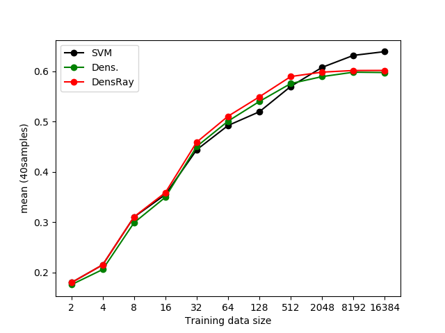
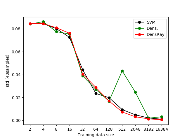
Table 1 shows results. As expected the performance of Densifier and DensRay is comparable (macro mean deviation of 0.001). We explain slight deviations between the results with the slightly different objective functions of DensRay and Densifier. In addition, the re-orthogonalization used in Densifier can result in an unstable training process. Figure 1 assesses the stability by reporting mean and standard deviation for the concreteness task (BWK lexicon). We varied the size of the training lexicon as depicted on the x-axis and sampled 40 subsets of the lexicon with the prescribed size. For the sizes 512 and 2048 Densifier shows an increased standard deviation. This is because there is at least one sample for which the performance significantly drops. Removing the re-orthogonalization in Densifier prevents the drop and restores performance. Recent work Zhao and Schütze (2019) also finds that replacing the orthogonalization with a regularization is reasonable in certain circumstances. Given that DensRay and Densifier yield the same performance and DensRay is a stable closed form solution always yielding a orthogonal transformation we conclude that DensRay is preferable.

Surprisingly, simple linear SVMs perform best in the task of lexicon induction. SVR is slightly better when continuous lexica are used for training (line 8). Note that the eigendecomposition used in DensRay yields a basis with dimensions ordered by their correlation with the linguistic feature. An SVM can achieve this only by iterated application.

	Task	Emb.	Lex. (Train)	Lex. (Test)	Dens.	DensRay	SVR	SVM
1	sent	CZ	SubLex	SubLex	0.546	0.549	0.585	0.585
2	sent	DE	GermanPC	GermanPC	0.636	0.631	0.674	0.677
3	sent	ES	fullstrength	fullstrength	0.541	0.546	0.571	0.576
4	sent	FR	FEEL	FEEL	0.469	0.471	0.555	0.565
5	sent	EN	WHM	WHM	0.623	0.623	0.627	0.625
6	sent	EN(t)	WHM	SE Trial*	0.624	0.621	0.618	0.637
7	sent	EN(t)	WHM	SE Test*	0.600	0.608	0.619	0.636
8	conc	EN	BWK*	BWK*	0.599	0.602	0.655	0.641
9	Macro Mean				0.580	0.581	0.613	0.618

Table 1: Results on lexicon induction. Numbers are Kendall

\tau

rank correlation. For details on the resources see Table 2 and Rothe et al. (2016). Bold: best result across methods. ^⋆: continuous lexicon.

Name	Description
CZ, DE, ES	Czech, German, Spanish embeddings by Rothe et al. (2016)
FR	French frWac embeddings Fauconnier (2015)
EN	English GoogleNews embeddings Mikolov et al. (2013)
EN(t)	English Twitter Embeddings Rothe et al. (2016)

Name	Description
SubLex	Czech sentiment lexicon Veselovská and Bojar (2013)
GermanPC	German sentiment lexicon Waltinger (2010)
fullstrength	Spanish sentiment lexicon Perez-Rosas et al. (2012)
FEEL	French sentiment lexicon Abdaoui et al. (2017)
WHM	English sentiment lexicon; combination of MPQA Wilson et al. (2005), Opinion Lexicon Hu and Liu (2004) and NRC emotion lexcion Mohammad and Turney (2013)
SE	Semeval 2015 Task 10E shared task data Rosenthal et al. (2015)
BWK	English concreteness lexicon Brysbaert et al. (2014)

Table 2: Overview of resources for lexicon induction. The setup is identical to Rothe et al. (2016).

Refer to caption — Figure 1: Mean (top) and standard deviation (bottom) of the performance across 40 samples of the training lexicon with varying sizes. Performed on the English concreteness task (line 8 in Table 1). SVR performs similar to SVM and is omitted for clarity.

4 Removing Gender Bias

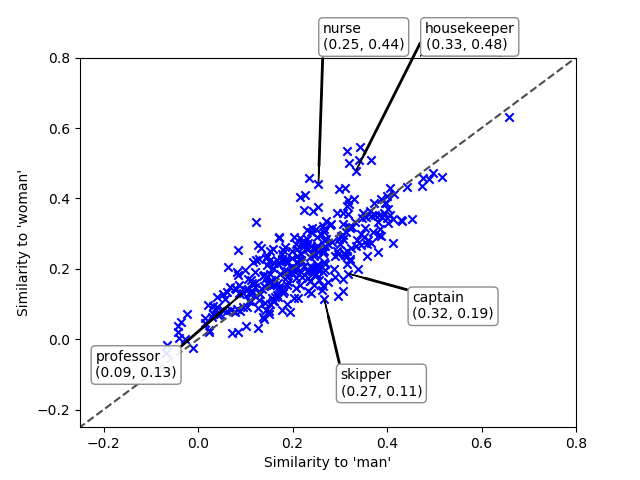
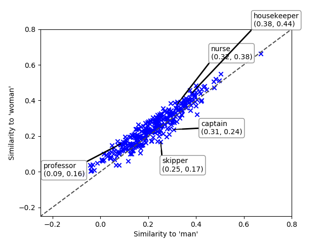
Word embeddings are well-known for encoding prevalent biases and stereotypes (cf. Bolukbasi et al. (2016)). We demonstrate qualitatively that by identifying an interpretable gender dimension and subsequently removing this dimension, one can remove parts of gender information that potentially could cause biases in downstream processing. Given the original word space $E$ we consider the interpretable space $E^{\prime}:=EQ$ , where $Q$ is computed using DensRay. We denote by $E_{\cdot,-1}\in\mathbb{R}^{n\times(d-1)}$ the word space with removed first dimension and call it the “complement” space. We expect $E_{\cdot,-1}$ to be a word space with less gender bias.

To examine this approach qualitatively we use a list of occupation names³³3https://github.com/tolga-b/debiaswe/blob/master/data/professions.json by Bolukbasi et al. (2016) and examine the cosine similarities of occupations with the vectors of “man” and “woman”. Figure 2 shows the similarities in the original space $E$ and debiased space $E_{\cdot,-1}$ . One can see the similarities are closer to the identity (i.e., same distance to “man” and “woman”) in the complement space. To identify occupations with the greatest bias, Table 3 lists occupations for which $\text{sim}(e_{w},e_{\text{man}})-\text{sim}(e_{w},e_{\text{woman}})$ is largest/smallest. One can clearly see a debiasing effect when considering the complement space. Extending this qualitative study to a more rigorous quantitative evaluation is part of future work.

	Original Space			Complement Space
		man	woman		man	woman
female bias	actress	0.23	0.46	lawyer	0.16	0.27
	businesswoman	0.32	0.53	ambassador	0.07	0.17
	registered_nurse	0.12	0.33	attorney	0.05	0.15
	housewife	0.34	0.55	legislator	0.26	0.36
	homemaker	0.22	0.40	minister	0.10	0.20
	…
male bias	hitman	0.41	0.27	captain	0.31	0.24
	gangster	0.34	0.20	marksman	0.29	0.21
	skipper	0.27	0.11	maestro	0.28	0.20
	marksman	0.31	0.14	hitman	0.40	0.32
	maestro	0.30	0.12	skipper	0.25	0.17

Table 3: Top 5 occupations that exhibit the greatest bias (measured by difference in cosine similarity). Numbers indicate cosine similarity between word vectors.

5 Word Analogy

In this section we use interpretable word spaces for set-based word analogy. Given a list of analogy pairs [( $a$ , $a^{\prime}$ ), ( $b$ , $b^{\prime}$ ), ( $c$ , $c^{\prime}$ ), …] the task is to predict $a^{\prime}$ given $a$ . Drozd et al. (2016) provide a detailed overview over different methods, and find that their method LRCos performs best.

LRCos assumes two classes: all left elements of a pair (“left class”) and all right elements (“right class”). They train a logistic regression (LR) to differentiate between these two classes. The predicted score of the LR multiplied by the cosine similarity in the word space is their final score. Their prediction for $a^{\prime}$ is the word with the highest final score.

We train the classifier on all analogy pairs except for a single pair for which we then obtain the predicted score. In addition we ensure that no word belonging to the test analogy is used during training (splitting the data only on word analogy pairs is not sufficient).

Inspired by LRCos we use interpretable word spaces for approaching word analogy: we train DensRay or an SVM to obtain interpretable embeddings $E^{\prime}=EQ$ using the class information as reasoned above. We use a slightly different notation in this section: for a word $w$ the $i$ th component of its embedding is given by $E_{w,i}$ . Therefore we denote as $E_{\cdot,1}$ the first column of $E^{\prime}$ (i.e., the most interpretable dimension). We min-max normalize $E_{\cdot,1}$ such that words belonging to the right class have a high value (i.e., we flip the sign if necessary). For a query word $a$ we now want to identify the corresponding $a^{\prime}$ by solving

\hat{a}=\arg\max_{v\in V}\;\text{norm}(E_{v,1})\,\text{sim}(E_{a,\cdot},E_{v,\cdot})

where sim computes the cosine similarity.

Given the result from §4 we extend the above method by computing the cosine similarity in the orthogonal complement, i.e., $\text{sim}(E_{a,-1},E_{v,-1})$ . We call this method IntCos (INTerpretable, COSine). Depending on the space used for computing the cosine similarity add the word “Original” or “Complement”.

We evaluate this method across two analogy datasets. These are the Google Analogy Dataset (GA) Mikolov et al. (2013) and BATS Drozd et al. (2016). As embeddings spaces we use Google News Embeddings (GN) Mikolov et al. (2013) and FastText subword embeddings (FT) Bojanowski et al. (2017). We consider the first 80k word embeddings from each space.

Table 4 shows the results. The first observation is that there is no clear winner. IntCos Original performs comparably to LRCos with slight improvements for GN/BATS: here the classes are widespread and exhibit low cosine similarity (IntraR and IntraL), which makes them harder to solve. IntCos Complement maintains performance for GN/BATS and is beneficial for Derivational analogies on GN. For most other analogies it harms performance.

Within IntCos Original it is favorable to use DensRay as it gives slight performance improvements. Especially for harder analogies, where interclass similarity is high and intraclass similarities are low (e.g., in GN/BATS), DensRay outperforms SVMs. In contrast to SVMs, DensRay considers difference vectors within classes as well – this seems to be of advantage here.

		Mean Cosine Sim			Precision
					IntCos				LRCos
					complement		original
		Inter	IntraL	IntraR	DensR.	SVM	DensR.	SVM
FT/BATS	Inflectional	0.75	0.48	0.51	0.92	0.93	0.97	0.97	0.97
	Derivational	0.63	0.47	0.45	0.74	0.78	0.81	0.80	0.80
	Encyclopedia	0.48	0.43	0.55	0.30	0.43	0.41	0.43	0.45
	Lexicography	0.62	0.37	0.38	0.17	0.20	0.21	0.22	0.26
	Macro Mean	0.62	0.44	0.47	0.53	0.58	0.60	0.60	0.61
	Macro Std	0.12	0.06	0.09	0.34	0.33	0.34	0.33	0.32
GN/BATS	Inflectional	0.63	0.22	0.23	0.88	0.87	0.88	0.88	0.88
	Derivational	0.44	0.21	0.20	0.55	0.50	0.51	0.48	0.44
	Encyclopedia	0.35	0.29	0.42	0.33	0.35	0.35	0.32	0.34
	Lexicography	0.45	0.17	0.18	0.19	0.17	0.19	0.17	0.18
	Macro Mean	0.46	0.22	0.26	0.48	0.47	0.48	0.46	0.45
	Macro Std	0.14	0.07	0.12	0.31	0.31	0.32	0.32	0.32
FT/GA	Micro Mean	0.73	0.48	0.53	0.88	0.91	0.93	0.92	0.93
	Macro Mean	0.71	0.50	0.53	0.87	0.90	0.91	0.90	0.89
	Macro Std	0.11	0.05	0.06	0.11	0.08	0.12	0.17	0.23
GN/GA	Micro Mean	0.62	0.31	0.36	0.85	0.87	0.89	0.87	0.88
	Macro Mean	0.61	0.30	0.35	0.85	0.86	0.88	0.85	0.87
	Macro Std	0.10	0.09	0.10	0.08	0.07	0.09	0.11	0.11

Table 4: Left part shows mean cosine similarity. Inter: mean cosine similarity between pairs. IntraL/R: mean cosine similarity within the left/right class. Right part shows precision for word analogy task.

6 Related Work

Identifying Interpretable Dimensions. Most relevant to our method is a line of work that uses transformations of existing word spaces to obtain interpretable subspaces. Rothe et al. (2016) compute an orthogonal transformation using shallow neural networks. Park et al. (2017) apply exploratory factor analysis to embedding spaces to obtain interpretable dimensions in an unsupervised manner. Their approach relies on solving complex optimization problems, while we focus on closed form solutions. Senel et al. (2018) use SEMCAT categories in combination with the Bhattacharya distance to identify interpretable directions. Also, oriented PCA Diamantaras and Kung (1996) is closely related to our method. However, both methods yield non-orthogonal transformation. Faruqui et al. (2015a) use semantic lexicons to retrofit embedding spaces. Thus they do not fully maintain the structure of the word space, which is in contrast to this work.

Interpretable Embedding Algorithms. Another line of work modifies embedding algorithms to yield interpretable dimensions Koç et al. (2018); Luo et al. (2015); Shin et al. (2018); Zhao et al. (2018). There is also much work that generates sparse embeddings that are claimed to be more interpretable Murphy et al. (2012); Faruqui et al. (2015b); Fyshe et al. (2015); Subramanian et al. (2018). Instead of learning new embeddings, we aim at making dense embeddings interpretable.

7 Conclusion

We investigated analytical methods for obtaining interpretable word spaces. Relevant methods were examined with the tasks of lexicon induction, word analogy and debiasing. We gratefully acknowledge funding through a Zentrum Digitalisierung.Bayern fellowship awarded to the first author. This work was supported by the European Research Council (# 740516). We thank the anonymous reviewers for valuable comments.

References

Abdaoui et al. (2017) Amine Abdaoui, Jérôme Azé, Sandra Bringay, and Pascal Poncelet. 2017. Feel: a french expanded emotion lexicon. Language Resources and Evaluation, 51(3).
Amir et al. (2015) Silvio Amir, Ramón Astudillo, Wang Ling, Bruno Martins, Mario J Silva, and Isabel Trancoso. 2015. Inesc-id: A regression model for large scale twitter sentiment lexicon induction. In Proceedings of the 9th International Workshop on Semantic Evaluation (SemEval 2015).
Bojanowski et al. (2017) Piotr Bojanowski, Edouard Grave, Armand Joulin, and Tomas Mikolov. 2017. Enriching word vectors with subword information. Transactions of the Association for Computational Linguistics.
Bolukbasi et al. (2016) Tolga Bolukbasi, Kai-Wei Chang, James Y Zou, Venkatesh Saligrama, and Adam T Kalai. 2016. Man is to computer programmer as woman is to homemaker? debiasing word embeddings. In Advances in Neural Information Processing Systems.
Brysbaert et al. (2014) Marc Brysbaert, Amy Beth Warriner, and Victor Kuperman. 2014. Concreteness ratings for 40 thousand generally known english word lemmas. Behavior research methods, 46(3).
Diamantaras and Kung (1996) Konstantinos I Diamantaras and Sun Yuan Kung. 1996. Principal component neural networks: theory and applications, volume 5. Wiley New York.
Drozd et al. (2016) Aleksandr Drozd, Anna Gladkova, and Satoshi Matsuoka. 2016. Word embeddings, analogies, and machine learning: Beyond king-man+ woman= queen. In Proceedings of COLING 2016, the 26th International Conference on Computational Linguistics: Technical Papers.
Faruqui et al. (2015a) Manaal Faruqui, Jesse Dodge, Sujay Kumar Jauhar, Chris Dyer, Eduard Hovy, and Noah A Smith. 2015a. Retrofitting word vectors to semantic lexicons. In Proceedings of the 2015 Conference of the North American Chapter of the Association for Computational Linguistics: Human Language Technologies.
Faruqui et al. (2015b) Manaal Faruqui, Yulia Tsvetkov, Dani Yogatama, Chris Dyer, and Noah A Smith. 2015b. Sparse overcomplete word vector representations. In Proceedings of the 53rd Annual Meeting of the Association for Computational Linguistics and the 7th International Joint Conference on Natural Language Processing.
Fauconnier (2015) Jean-Philippe Fauconnier. 2015. French word embeddings.
Fyshe et al. (2015) Alona Fyshe, Leila Wehbe, Partha P Talukdar, Brian Murphy, and Tom M Mitchell. 2015. A compositional and interpretable semantic space. In Proceedings of the 2015 Conference of the North American Chapter of the Association for Computational Linguistics: Human Language Technologies.
Horn et al. (1990) Roger A Horn, Roger A Horn, and Charles R Johnson. 1990. Matrix analysis. Cambridge university press.
Hu and Liu (2004) Minqing Hu and Bing Liu. 2004. Mining and summarizing customer reviews. In Proceedings of the tenth ACM SIGKDD international conference on Knowledge discovery and data mining.
Koç et al. (2018) Aykut Koç, Ihsan Utlu, Lutfi Kerem Senel, and Haldun M Ozaktas. 2018. Imparting interpretability to word embeddings. arXiv preprint arXiv:1807.07279.
Luo et al. (2015) Hongyin Luo, Zhiyuan Liu, Huanbo Luan, and Maosong Sun. 2015. Online learning of interpretable word embeddings. In Proceedings of the 2015 Conference on Empirical Methods in Natural Language Processing.
Mikolov et al. (2013) Tomas Mikolov, Kai Chen, Greg Corrado, and Jeffrey Dean. 2013. Efficient estimation of word representations in vector space. arXiv preprint arXiv:1301.3781.
Mohammad and Turney (2013) Saif M Mohammad and Peter D Turney. 2013. Crowdsourcing a word–emotion association lexicon. Computational Intelligence, 29(3).
Murphy et al. (2012) Brian Murphy, Partha Talukdar, and Tom Mitchell. 2012. Learning effective and interpretable semantic models using non-negative sparse embedding. Proceedings of the 24th International Conference on Computational Linguistics.
Park et al. (2017) Sungjoon Park, JinYeong Bak, and Alice Oh. 2017. Rotated word vector representations and their interpretability. In Proceedings of the 2017 Conference on Empirical Methods in Natural Language Processing.
Perez-Rosas et al. (2012) Veronica Perez-Rosas, Carmen Banea, and Rada Mihalcea. 2012. Learning sentiment lexicons in spanish. In Proceedings of the seventh international conference on Language Resources and Evaluation.
Rosenthal et al. (2015) Sara Rosenthal, Preslav Nakov, Svetlana Kiritchenko, Saif Mohammad, Alan Ritter, and Veselin Stoyanov. 2015. Semeval-2015 task 10: Sentiment analysis in twitter. In Proceedings of the 9th international workshop on semantic evaluation.
Rothe et al. (2016) Sascha Rothe, Sebastian Ebert, and Hinrich Schütze. 2016. Ultradense word embeddings by orthogonal transformation. In Proceedings of the 2016 Conference of the North American Chapter of the Association for Computational Linguistics: Human Language Technologies.
Senel et al. (2018) Lutfi Kerem Senel, Ihsan Utlu, Veysel Yucesoy, Aykut Koc, and Tolga Cukur. 2018. Semantic structure and interpretability of word embeddings. IEEE/ACM Transactions on Audio, Speech, and Language Processing.
Shin et al. (2018) Jamin Shin, Andrea Madotto, and Pascale Fung. 2018. Interpreting word embeddings with eigenvector analysis. openreview.net.
Subramanian et al. (2018) Anant Subramanian, Danish Pruthi, Harsh Jhamtani, Taylor Berg-Kirkpatrick, and Eduard Hovy. 2018. Spine: Sparse interpretable neural embeddings. In Thirty-Second AAAI Conference on Artificial Intelligence.
Veselovská and Bojar (2013) Kateřina Veselovská and Ondřej Bojar. 2013. Czech sublex 1.0. Charles University, Faculty of Mathematics and Physics.
Waltinger (2010) Ulli Waltinger. 2010. Germanpolarityclues: A lexical resource for german sentiment analysis. In Proceedings of the seventh international conference on Language Resources and Evaluation.
Wilson et al. (2005) Theresa Wilson, Janyce Wiebe, and Paul Hoffmann. 2005. Recognizing contextual polarity in phrase-level sentiment analysis. In Proceedings of Human Language Technology Conference and Conference on Empirical Methods in Natural Language Processing.
Zhao et al. (2018) Jieyu Zhao, Yichao Zhou, Zeyu Li, Wei Wang, and Kai-Wei Chang Chang. 2018. Learning gender-neutral word embeddings. In Proceedings of the 2018 Conference on Empirical Methods in Natural Language Processing.
Zhao and Schütze (2019) Mengjie Zhao and Hinrich Schütze. 2019. A multilingual bpe embedding space for universal sentiment lexicon induction. In Proceedings of the 57th Conference of the Association for Computational Linguistics.

8 Appendix

8.1 Code

The code which was used to conduct the experiments in this paper is available at https://github.com/pdufter/densray.

8.2 Continuous Lexicon

In case of a continuous lexicon $l:V\to\mathbb{R}$ one can extend Equation 2 in the main paper by defining:

A:=\sum_{(v,w)\in V\times V}-l(v)l(w)d_{vw}d_{vw}^{\intercal}

In the case of a binary lexicon Equation 2 from the main paper is recovered for $\alpha_{\not=}=\alpha_{=}=1$ .

8.3 Full Analogy Results

In this section we present the results of the word analogy task per category. See Table 5 and Table 6 for detailed results with the methods IntCos Complement and Original, respectively. The format and numbers presented are the same as in the corresponding table from the main paper.

FastText

Google News

Google Analogy

	Mean Cosine Sim			Precision
				IntCos		LRCos
	Inter	IntraL	IntraR	DensRay	SVM
capital-common-countries	0.76	0.53	0.56	1.00	1.00	1.00
capital-world	0.75	0.44	0.51	0.97	0.96	1.00
city-in-state	0.71	0.51	0.63	0.78	0.79	0.85
currency	0.33	0.59	0.48	0.62	0.69	0.08
family	0.84	0.57	0.59	0.91	0.91	0.95
gram1-adjective-to-adverb	0.66	0.50	0.56	0.78	0.84	0.88
gram2-opposite	0.72	0.51	0.54	0.69	0.83	0.76
gram3-comparative	0.75	0.53	0.57	0.84	0.89	0.95
gram4-superlative	0.70	0.53	0.61	0.94	1.00	1.00
gram5-present-participle	0.76	0.43	0.48	1.00	0.94	1.00
gram6-nationality-adjective	0.70	0.55	0.54	0.90	0.90	0.93
gram7-past-tense	0.73	0.49	0.47	0.82	0.90	0.97
gram8-plural	0.80	0.41	0.42	1.00	1.00	1.00
gram9-plural-verbs	0.74	0.43	0.48	0.90	0.97	1.00
Micro Mean	0.73	0.48	0.53	0.88	0.91	0.93
Macro Mean	0.71	0.50	0.53	0.87	0.90	0.89
Macro Std	0.11	0.05	0.06	0.11	0.08	0.23

	Mean Cosine Sim			Precision
				IntCos		LRCos
	Inter	IntraL	IntraR	DensRay	SVM
capital-common-countries	0.64	0.37	0.38	0.91	0.96	0.91
capital-world	0.64	0.34	0.36	0.86	0.88	0.90
city-in-state	0.59	0.37	0.49	0.82	0.85	0.87
currency	0.37	0.42	0.44	0.78	0.72	0.56
family	0.74	0.48	0.53	0.83	0.87	0.87
gram1-adjective-to-adverb	0.49	0.21	0.26	0.69	0.75	0.75
gram2-opposite	0.50	0.24	0.31	0.68	0.75	0.71
gram3-comparative	0.60	0.25	0.40	0.92	0.92	0.97
gram4-superlative	0.54	0.26	0.39	0.97	0.91	0.94
gram5-present-participle	0.70	0.20	0.21	0.88	0.88	0.94
gram6-nationality-adjective	0.72	0.41	0.41	0.95	0.95	0.93
gram7-past-tense	0.66	0.21	0.22	0.82	0.82	0.85
gram8-plural	0.73	0.21	0.23	0.92	0.89	0.97
gram9-plural-verbs	0.64	0.22	0.24	0.87	0.90	0.93
Micro Mean	0.62	0.31	0.36	0.85	0.87	0.88
Macro Mean	0.61	0.30	0.35	0.85	0.86	0.87
Macro Std	0.10	0.09	0.10	0.08	0.07	0.11

BATS

	Mean Cosine Sim			Precision
				IntCos		LRCos
	Inter	IntraL	IntraR	DensRay	SVM
Derivational	0.63	0.47	0.45	0.74	0.78	0.80
D01 [noun+less-reg]	0.51	0.36	0.45	0.50	0.53	0.60
D02 [un+adj-reg]	0.71	0.46	0.46	0.68	0.72	0.84
D03 [adj+ly-reg]	0.63	0.50	0.52	0.86	0.88	0.90
D04 [over+adj-reg]	0.63	0.45	0.45	0.59	0.69	0.62
D05 [adj+ness-reg]	0.63	0.49	0.51	0.92	1.00	0.92
D06 [re+verb-reg]	0.74	0.52	0.49	0.50	0.62	0.76
D07 [verb+able-reg]	0.57	0.48	0.45	0.71	0.66	0.63
D08 [verb+er-irreg]	0.55	0.48	0.41	0.84	0.88	0.79
D09 [verb+tion-irreg]	0.63	0.46	0.41	0.86	0.88	0.86
D10 [verb+ment-irreg]	0.64	0.46	0.42	0.86	0.88	0.90
Encyclopedia	0.48	0.43	0.55	0.30	0.43	0.45
E01 [country - capital]	0.63	0.47	0.41	0.72	0.96	0.98
E02 [country - language]	0.40	0.43	0.59	0.24	0.35	0.33
E03 [UK-city - county]	0.59	0.49	0.57	0.22	0.36	0.36
E04 [name - nationality]	0.28	0.39	0.64	0.45	0.66	0.60
E05 [name - occupation]	0.44	0.41	0.57	0.42	0.65	0.73
E06 [animal - young]	0.47	0.43	0.44	0.05	0.07	0.15
E07 [animal - sound]	0.37	0.43	0.40	0.15	0.20	0.22
E08 [animal - shelter]	0.44	0.42	0.51	0.00	0.07	0.13
E09 [things - color]	0.44	0.38	0.81	0.04	0.22	0.16
E10 [male - female]	0.73	0.43	0.43	0.68	0.68	0.78
Inflectional	0.75	0.48	0.51	0.92	0.93	0.97
I01 [noun - plural-reg]	0.79	0.39	0.41	0.98	1.00	1.00
I02 [noun - plural-irreg]	0.77	0.40	0.42	0.80	0.80	0.84
I03 [adj - comparative]	0.75	0.50	0.52	0.97	1.00	1.00
I04 [adj - superlative]	0.71	0.51	0.58	0.96	0.96	1.00
I05 [verb-inf - 3pSg]	0.77	0.52	0.53	0.96	0.98	1.00
I06 [verb-inf - Ving]	0.77	0.51	0.51	0.80	0.88	0.96
I07 [verb-inf - Ved]	0.75	0.51	0.55	0.92	0.94	1.00
I08 [verb-Ving - 3pSg]	0.70	0.48	0.51	0.94	0.96	0.98
I09 [verb-Ving - Ved]	0.73	0.50	0.54	0.92	0.88	0.98
I10 [verb-3pSg - Ved]	0.72	0.53	0.55	0.96	0.96	1.00
Lexicography	0.62	0.37	0.38	0.17	0.20	0.26
L01 [hypernyms - animals]	0.58	0.43	0.53	0.02	0.29	0.24
L02 [hypernyms - misc]	0.55	0.35	0.39	0.14	0.11	0.14
L03 [hyponyms - misc]	0.63	0.35	0.31	0.28	0.28	0.28
L04 [meronyms - substance]	0.53	0.36	0.44	0.15	0.21	0.17
L05 [meronyms - member]	0.58	0.36	0.36	0.10	0.10	0.12
L06 [meronyms - part]	0.53	0.31	0.30	0.04	0.09	0.09
L07 [synonyms - intensity]	0.67	0.37	0.37	0.25	0.25	0.36
L08 [synonyms - exact]	0.71	0.33	0.31	0.18	0.16	0.22
L09 [antonyms - gradable]	0.68	0.45	0.43	0.35	0.33	0.55
L10 [antonyms - binary]	0.72	0.40	0.40	0.18	0.18	0.39
Micro Mean	0.62	0.44	0.47	0.52	0.58	0.61
Macro Mean	0.62	0.44	0.47	0.53	0.58	0.61
Macro Std	0.12	0.06	0.09	0.34	0.33	0.32

	Mean Cosine Sim			Precision
				IntCos		LRCos
	Inter	IntraL	IntraR	DensRay	SVM
Derivational	0.44	0.21	0.20	0.55	0.50	0.44
D01 [noun+less-reg]	0.26	0.16	0.24	0.14	0.14	0.05
D02 [un+adj-reg]	0.47	0.17	0.20	0.66	0.54	0.58
D03 [adj+ly-reg]	0.48	0.17	0.22	0.70	0.76	0.76
D04 [over+adj-reg]	0.39	0.17	0.21	0.41	0.44	0.30
D05 [adj+ness-reg]	0.47	0.21	0.26	0.75	0.75	0.65
D06 [re+verb-reg]	0.56	0.29	0.28	0.64	0.53	0.58
D07 [verb+able-reg]	0.38	0.25	0.20	0.38	0.28	0.19
D08 [verb+er-irreg]	0.30	0.24	0.17	0.29	0.19	0.07
D09 [verb+tion-irreg]	0.51	0.22	0.15	0.73	0.63	0.51
D10 [verb+ment-irreg]	0.47	0.24	0.15	0.60	0.56	0.44
Encyclopedia	0.35	0.29	0.42	0.33	0.35	0.34
E01 [country - capital]	0.61	0.35	0.32	0.88	0.90	0.90
E02 [country - language]	0.36	0.31	0.45	0.47	0.30	0.36
E03 [UK-city - county]	0.41	0.36	0.52	0.14	0.14	0.14
E04 [name - nationality]	0.20	0.20	0.39	0.33	0.33	0.26
E05 [name - occupation]	0.33	0.21	0.40	0.45	0.62	0.52
E06 [animal - young]	0.34	0.36	0.38	0.06	0.06	0.12
E07 [animal - sound]	0.15	0.31	0.25	0.17	0.03	0.00
E08 [animal - shelter]	0.25	0.29	0.39	0.00	0.16	0.09
E09 [things - color]	0.20	0.23	0.63	0.08	0.15	0.21
E10 [male - female]	0.62	0.28	0.33	0.66	0.68	0.68
Inflectional	0.63	0.22	0.23	0.88	0.87	0.88
I01 [noun - plural-reg]	0.69	0.13	0.16	0.84	0.84	0.88
I02 [noun - plural-irreg]	0.62	0.12	0.16	0.67	0.69	0.75
I03 [adj - comparative]	0.63	0.23	0.37	0.97	0.97	1.00
I04 [adj - superlative]	0.59	0.26	0.39	0.93	0.93	0.97
I05 [verb-inf - 3pSg]	0.65	0.26	0.33	1.00	1.00	1.00
I06 [verb-inf - Ving]	0.67	0.26	0.19	0.84	0.82	0.82
I07 [verb-inf - Ved]	0.66	0.25	0.20	0.92	0.90	0.88
I08 [verb-Ving - 3pSg]	0.56	0.17	0.31	0.90	0.92	0.90
I09 [verb-Ving - Ved]	0.64	0.18	0.19	0.84	0.84	0.82
I10 [verb-3pSg - Ved]	0.62	0.33	0.20	0.90	0.88	0.88
Lexicography	0.45	0.17	0.18	0.19	0.17	0.18
L01 [hypernyms - animals]	0.47	0.32	0.47	0.00	0.05	0.05
L02 [hypernyms - misc]	0.42	0.21	0.21	0.29	0.21	0.10
L03 [hyponyms - misc]	0.52	0.15	0.15	0.19	0.14	0.14
L04 [meronyms - substance]	0.35	0.16	0.24	0.15	0.09	0.11
L05 [meronyms - member]	0.36	0.15	0.15	0.10	0.08	0.08
L06 [meronyms - part]	0.34	0.14	0.12	0.09	0.09	0.02
L07 [synonyms - intensity]	0.51	0.17	0.16	0.24	0.26	0.30
L08 [synonyms - exact]	0.55	0.11	0.11	0.15	0.15	0.22
L09 [antonyms - gradable]	0.45	0.18	0.19	0.41	0.41	0.43
L10 [antonyms - binary]	0.50	0.14	0.15	0.21	0.17	0.31
Micro Mean	0.47	0.22	0.26	0.49	0.48	0.47
Macro Mean	0.46	0.22	0.26	0.48	0.47	0.45
Macro Std	0.14	0.07	0.12	0.31	0.31	0.32

Table 5: Detailed results for all combinations of FastText/Google News embeddings and Google Analogy and BATS analogies. In this table the cosine similarity is computed in the orthogonal complement. See the main paper for more details.

FastText

Google News

Google Analogy

	Mean Cosine Sim			Precision
				IntCos		LRCos
	Inter	IntraL	IntraR	DensRay	SVM
capital-common-countries	0.76	0.53	0.56	1.00	1.00	1.00
capital-world	0.75	0.44	0.51	0.98	0.98	1.00
city-in-state	0.71	0.51	0.63	0.87	0.85	0.85
currency	0.33	0.59	0.48	0.54	0.31	0.08
family	0.84	0.57	0.59	0.91	0.91	0.95
gram1-adjective-to-adverb	0.66	0.50	0.56	0.88	0.84	0.88
gram2-opposite	0.72	0.51	0.54	0.72	0.83	0.76
gram3-comparative	0.75	0.53	0.57	0.92	0.95	0.95
gram4-superlative	0.70	0.53	0.61	1.00	1.00	1.00
gram5-present-participle	0.76	0.43	0.48	1.00	1.00	1.00
gram6-nationality-adjective	0.70	0.55	0.54	0.93	0.93	0.93
gram7-past-tense	0.73	0.49	0.47	0.95	0.93	0.97
gram8-plural	0.80	0.41	0.42	1.00	1.00	1.00
gram9-plural-verbs	0.74	0.43	0.48	1.00	1.00	1.00
Micro Mean	0.73	0.48	0.53	0.93	0.92	0.93
Macro Mean	0.71	0.50	0.53	0.91	0.90	0.89
Macro Std	0.11	0.05	0.06	0.12	0.17	0.23

	Mean Cosine Sim			Precision
				IntCos		LRCos
	Inter	IntraL	IntraR	DensRay	SVM
capital-common-countries	0.64	0.37	0.38	0.91	0.91	0.91
capital-world	0.64	0.34	0.36	0.90	0.90	0.90
city-in-state	0.59	0.37	0.49	0.85	0.88	0.87
currency	0.37	0.42	0.44	0.67	0.50	0.56
family	0.74	0.48	0.53	0.87	0.87	0.87
gram1-adjective-to-adverb	0.49	0.21	0.26	0.78	0.75	0.75
gram2-opposite	0.50	0.24	0.31	0.71	0.75	0.71
gram3-comparative	0.60	0.25	0.40	0.97	0.95	0.97
gram4-superlative	0.54	0.26	0.39	0.94	0.94	0.94
gram5-present-participle	0.70	0.20	0.21	0.94	0.91	0.94
gram6-nationality-adjective	0.72	0.41	0.41	0.93	0.93	0.93
gram7-past-tense	0.66	0.21	0.22	0.88	0.85	0.85
gram8-plural	0.73	0.21	0.23	0.97	0.89	0.97
gram9-plural-verbs	0.64	0.22	0.24	0.93	0.87	0.93
Micro Mean	0.62	0.31	0.36	0.89	0.87	0.88
Macro Mean	0.61	0.30	0.35	0.88	0.85	0.87
Macro Std	0.10	0.09	0.10	0.09	0.11	0.11

BATS

	Mean Cosine Sim			Precision
				IntCos		LRCos
	Inter	IntraL	IntraR	DensRay	SVM
Derivational	0.63	0.47	0.45	0.81	0.80	0.80
D01 [noun+less-reg]	0.51	0.36	0.45	0.60	0.60	0.60
D02 [un+adj-reg]	0.71	0.46	0.46	0.80	0.72	0.84
D03 [adj+ly-reg]	0.63	0.50	0.52	0.90	0.90	0.90
D04 [over+adj-reg]	0.63	0.45	0.45	0.66	0.69	0.62
D05 [adj+ness-reg]	0.63	0.49	0.51	1.00	0.96	0.92
D06 [re+verb-reg]	0.74	0.52	0.49	0.59	0.71	0.76
D07 [verb+able-reg]	0.57	0.48	0.45	0.74	0.63	0.63
D08 [verb+er-irreg]	0.55	0.48	0.41	0.91	0.86	0.79
D09 [verb+tion-irreg]	0.63	0.46	0.41	0.91	0.93	0.86
D10 [verb+ment-irreg]	0.64	0.46	0.42	0.92	0.90	0.90
Encyclopedia	0.48	0.43	0.55	0.41	0.43	0.45
E01 [country - capital]	0.63	0.47	0.41	0.96	0.96	0.98
E02 [country - language]	0.40	0.43	0.59	0.33	0.24	0.33
E03 [UK-city - county]	0.59	0.49	0.57	0.30	0.42	0.36
E04 [name - nationality]	0.28	0.39	0.64	0.49	0.51	0.60
E05 [name - occupation]	0.44	0.41	0.57	0.75	0.73	0.73
E06 [animal - young]	0.47	0.43	0.44	0.10	0.15	0.15
E07 [animal - sound]	0.37	0.43	0.40	0.22	0.17	0.22
E08 [animal - shelter]	0.44	0.42	0.51	0.02	0.13	0.13
E09 [things - color]	0.44	0.38	0.81	0.12	0.22	0.16
E10 [male - female]	0.73	0.43	0.43	0.76	0.71	0.78
Inflectional	0.75	0.48	0.51	0.97	0.97	0.97
I01 [noun - plural-reg]	0.79	0.39	0.41	1.00	1.00	1.00
I02 [noun - plural-irreg]	0.77	0.40	0.42	0.84	0.82	0.84
I03 [adj - comparative]	0.75	0.50	0.52	1.00	1.00	1.00
I04 [adj - superlative]	0.71	0.51	0.58	0.96	0.96	1.00
I05 [verb-inf - 3pSg]	0.77	0.52	0.53	1.00	1.00	1.00
I06 [verb-inf - Ving]	0.77	0.51	0.51	0.96	0.96	0.96
I07 [verb-inf - Ved]	0.75	0.51	0.55	1.00	1.00	1.00
I08 [verb-Ving - 3pSg]	0.70	0.48	0.51	0.98	0.98	0.98
I09 [verb-Ving - Ved]	0.73	0.50	0.54	0.98	0.96	0.98
I10 [verb-3pSg - Ved]	0.72	0.53	0.55	1.00	1.00	1.00
Lexicography	0.62	0.37	0.38	0.21	0.22	0.26
L01 [hypernyms - animals]	0.58	0.43	0.53	0.20	0.37	0.24
L02 [hypernyms - misc]	0.55	0.35	0.39	0.23	0.16	0.14
L03 [hyponyms - misc]	0.63	0.35	0.31	0.33	0.28	0.28
L04 [meronyms - substance]	0.53	0.36	0.44	0.10	0.15	0.17
L05 [meronyms - member]	0.58	0.36	0.36	0.12	0.10	0.12
L06 [meronyms - part]	0.53	0.31	0.30	0.04	0.15	0.09
L07 [synonyms - intensity]	0.67	0.37	0.37	0.27	0.32	0.36
L08 [synonyms - exact]	0.71	0.33	0.31	0.18	0.16	0.22
L09 [antonyms - gradable]	0.68	0.45	0.43	0.43	0.37	0.55
L10 [antonyms - binary]	0.72	0.40	0.40	0.18	0.18	0.39
Micro Mean	0.62	0.44	0.47	0.59	0.60	0.61
Macro Mean	0.62	0.44	0.47	0.60	0.60	0.61
Macro Std	0.12	0.06	0.09	0.34	0.33	0.32

	Mean Cosine Sim			Precision
				IntCos		LRCos
	Inter	IntraL	IntraR	DensRay	SVM
Derivational	0.44	0.21	0.20	0.51	0.48	0.44
D01 [noun+less-reg]	0.26	0.16	0.24	0.10	0.10	0.05
D02 [un+adj-reg]	0.47	0.17	0.20	0.66	0.58	0.58
D03 [adj+ly-reg]	0.48	0.17	0.22	0.76	0.78	0.76
D04 [over+adj-reg]	0.39	0.17	0.21	0.41	0.41	0.30
D05 [adj+ness-reg]	0.47	0.21	0.26	0.75	0.70	0.65
D06 [re+verb-reg]	0.56	0.29	0.28	0.69	0.61	0.58
D07 [verb+able-reg]	0.38	0.25	0.20	0.28	0.22	0.19
D08 [verb+er-irreg]	0.30	0.24	0.17	0.12	0.10	0.07
D09 [verb+tion-irreg]	0.51	0.22	0.15	0.61	0.61	0.51
D10 [verb+ment-irreg]	0.47	0.24	0.15	0.54	0.50	0.44
Encyclopedia	0.35	0.29	0.42	0.35	0.32	0.34
E01 [country - capital]	0.61	0.35	0.32	0.90	0.90	0.90
E02 [country - language]	0.36	0.31	0.45	0.43	0.21	0.36
E03 [UK-city - county]	0.41	0.36	0.52	0.14	0.12	0.14
E04 [name - nationality]	0.20	0.20	0.39	0.26	0.15	0.26
E05 [name - occupation]	0.33	0.21	0.40	0.60	0.57	0.52
E06 [animal - young]	0.34	0.36	0.38	0.09	0.12	0.12
E07 [animal - sound]	0.15	0.31	0.25	0.08	0.00	0.00
E08 [animal - shelter]	0.25	0.29	0.39	0.07	0.14	0.09
E09 [things - color]	0.20	0.23	0.63	0.19	0.19	0.21
E10 [male - female]	0.62	0.28	0.33	0.68	0.68	0.68
Inflectional	0.63	0.22	0.23	0.88	0.88	0.88
I01 [noun - plural-reg]	0.69	0.13	0.16	0.86	0.84	0.88
I02 [noun - plural-irreg]	0.62	0.12	0.16	0.69	0.71	0.75
I03 [adj - comparative]	0.63	0.23	0.37	0.97	1.00	1.00
I04 [adj - superlative]	0.59	0.26	0.39	0.97	0.97	0.97
I05 [verb-inf - 3pSg]	0.65	0.26	0.33	1.00	1.00	1.00
I06 [verb-inf - Ving]	0.67	0.26	0.19	0.86	0.82	0.82
I07 [verb-inf - Ved]	0.66	0.25	0.20	0.92	0.90	0.88
I08 [verb-Ving - 3pSg]	0.56	0.17	0.31	0.90	0.90	0.90
I09 [verb-Ving - Ved]	0.64	0.18	0.19	0.84	0.82	0.82
I10 [verb-3pSg - Ved]	0.62	0.33	0.20	0.88	0.88	0.88
Lexicography	0.45	0.17	0.18	0.19	0.17	0.18
L01 [hypernyms - animals]	0.47	0.32	0.47	0.08	0.08	0.05
L02 [hypernyms - misc]	0.42	0.21	0.21	0.26	0.26	0.10
L03 [hyponyms - misc]	0.52	0.15	0.15	0.19	0.14	0.14
L04 [meronyms - substance]	0.35	0.16	0.24	0.09	0.09	0.11
L05 [meronyms - member]	0.36	0.15	0.15	0.10	0.06	0.08
L06 [meronyms - part]	0.34	0.14	0.12	0.09	0.09	0.02
L07 [synonyms - intensity]	0.51	0.17	0.16	0.26	0.26	0.30
L08 [synonyms - exact]	0.55	0.11	0.11	0.15	0.15	0.22
L09 [antonyms - gradable]	0.45	0.18	0.19	0.45	0.41	0.43
L10 [antonyms - binary]	0.50	0.14	0.15	0.19	0.17	0.31
Micro Mean	0.47	0.22	0.26	0.49	0.47	0.47
Macro Mean	0.46	0.22	0.26	0.48	0.46	0.45
Macro Std	0.14	0.07	0.12	0.32	0.32	0.32

Table 6: Detailed results for all combinations of FastText/Google News embeddings and Google Analogy and BATS analogies. In this table the cosine similarity is computed in the original space. See the main paper for more details.