1 Introduction

As is well known via triangulation, when we look at a point from two known viewpoints, we can then calculate where the point is. Let us turn our attention to the case of a surface. When we look at a surface, then we observe an apparent contour (a contour), which gives us some information about the surface. In fact, reconstructing objects in 3-space from the information of apparent contours is an important subject in the area of computer vision, computer graphics and visual perception [1, 2, 3, 7, 8, 10, 13, 14, 15, 22].

One cannot obtain complete information from a finite number of apparent contours, in general. However, to obtain the Gaussian curvature of a surface, information about the second order derivatives of the surface is required, and in [13, 14], Koenderink showed that one can obtain the Gaussian curvature of a surface as the product of the curvature of the contour and the normal curvature along a single direction. While Koenderink’s result needs more information than just the apparent contour, that is, it needs the normal curvature, this fact still suggests that we might be able to obtain some information about a surface from curvatures of small numbers of contours of the surface. It then is natural to ask how much information about the contour is enough to get the desired information about a surface.

In this paper, we consider an orthogonal projection of $\boldsymbol{R}^{3}$ to a plane:

$$\pi_{\xi}(x)=x-\left\langle{x},{\xi}\right\rangle\xi:\boldsymbol{R}^{3}\to\xi^{\perp}$$

for a unit vector $\xi\in\boldsymbol{R}^{3}$. The map $\pi_{\xi}$ is called the orthogonal projection in the direction $\xi$. Our interest is in getting local information on surfaces (or curves) from the curvatures of the contours (or the projected curves) with respect to orthogonal projections. In particular, we show how much information about contours (or image curves) is enough to recover the lower degree terms of the Taylor expansions of surfaces (or curves) at observed points. Note that we also give explicit formulae for reconstructing basic information of curves and surfaces from a finite number of projected images (see Remark 1.1). In addition, we construct some examples of sets of different surfaces whose information with respect to contours for certain orthogonal projections is exactly the same (Figures 3.3, 3.4, 3.5). See [1, 3, 4, 5, 6, 7, 15] for other approaches to these kinds of considerations.

Remark 1.1.

Explicit formulae for reconstructing information about surfaces and curves from their projected images are useful tools in practical settings. In addition to Koenderink’s famous result [13, 14] explained above, [10] provided a formula for recovering a surface from continuous data of the apparent contours. Their works have received attention in the context of visual perception and computer vision (cf. [1, 2, 3, 8, 22]). The formulae in the present paper are certain kinds of expansions of previous results [13, 14, 10], which are useful for reconstructing objects from a just few static images. We believe that our formulae are ready for use in practical applications where such a reconstruction is needed.

Throughout the paper, we use the following notation for the Taylor coefficients of a given function. For a $C^{\infty}$ function $\psi:I\to\boldsymbol{R}$, we set

$$(\operatorname{coef}_{0}(\psi,t,k)=)\operatorname{coef}(\psi,t,k)=\left(\psi(0),\psi^{\prime}(0),\dfrac{\psi^{\prime\prime}(0)}{2},\ldots,\dfrac{\psi^{(k)}(0)}{k!}\right)$$

(${~{}}^{\prime}=d/dt$ and $\psi^{(i)}=(\psi^{(i-1)})^{\prime}$ for $i=1,2,\ldots$), namely, if $h=a_{0}+\sum_{i=1}^{k}(a_{i}/i!)t^{i}$, then

$$\operatorname{coef}(\psi,t,k)=(a_{0},a_{1},a_{2}/2,\ldots,a_{k}/k!).$$

The data $\operatorname{coef}(\psi,t,k)$ is called the $k$-th order information of $\psi$ $($at $0)$. We remark that the $k$-th order information of the given function $\psi$ at $0$ represents the $k$-jet of $\psi$ at $0$ in the terminology of singularity theory (cf. [12]).

1.1 Projections of curves

Let $I$ be an open interval containing $0$, and let $\gamma:I\to\boldsymbol{R}^{3}$ ($\gamma(0)=(0,0,0)$) be a given unknown regular $C^{\infty}$ curve whose curvature does not vanish at $0$. We remark that $\gamma$ has the orientation induced from that of $I$. Rotating the coordinate system of $\boldsymbol{R}^{3}$ if necessary, for any $k\in\boldsymbol{N}$, we may assume that $\gamma$ is locally written around $0$ as

$$\gamma(t)=\left(t,\ \sum_{i=2}^{k}\dfrac{a_{i}}{i!}t^{i},\ \sum_{i=3}^{k}\dfrac{b_{i}}{i!}t^{i}\right)+(O(k+1),O(k+1),O(k+1)),$$ (1.1)

where $a_{i},b_{i}\in\boldsymbol{R}$ $(i=2,\ldots,k)$, and $O(k+1)$ stands for the terms whose degrees are greater than $k$. Specifically, $a_{2}$ and $b_{3}$ are important values of the space curve: the curvature and the torsion at $0$. Set $\gamma_{\xi}=\pi_{\xi}\circ\gamma$ for a unit vector $\xi\in\boldsymbol{R}^{3}$. Our aim is to investigate how many conditions are enough to recover the above coefficients in terms of the curvatures of $\gamma_{\xi}$ using a number of distinct directions $\xi$.

Since the setting is complicated for general choices of projection directions, we focus on the two singular cases where the kernel direction $\xi$ of an orthogonal projection is geometrically restricted. The following are our settings, and also abstracts of the results which will be given in Section 2:

• We take two linearly independent vectors $\xi_{1},\xi_{2}$, where each projected curve $\gamma_{\xi_{i}}$ $(i=1,2)$ has an inflection point at $0$. This implies that $\xi_{1},\xi_{2}$ lie in the osculating plane, with the exception of the tangent line of $\gamma$ (Figure 2.1). Then the coefficients $a_{i},b_{i}$ can be uniquely determined from the certain order of the information of the curvature functions of $\gamma_{\xi_{i}}$ $(i=1,2)$ at $0$ (Theorem 2.1). Namely, the coefficients $a_{i},b_{i}$ can be uniquely determined by the information of the derivatives of the curvatures of the two projected curves.

• We take $\xi_{1}$ as a tangent vector of $\gamma$ at $0$. Then, $\gamma_{\xi_{1}}=\pi_{\xi_{1}}\circ\gamma$ has a singular point at $0$ (Figure 2.2). We also take another vector $\xi_{2}$. Then the coefficients $a_{i},b_{i}$ ($i\leq 5$) can be uniquely determined by the information of the curvature functions of $\gamma_{\xi_{i}}$ $(i=1,2)$ at $0$. Namely, the coefficients $a_{i},b_{i}$ ($i\leq 5$) can be uniquely determined from the curvature functions of two projected curves from the tangential direction and another direction (Theorem 2.2). The notion of the cuspidal curvature of a singular plane curve (introduced in [20]), especially, plays an important role.

1.2 Projections of surfaces

Let $U$ be an open subset of $\boldsymbol{R}^{2}$ containing $0=(0,0)$, and let $f:U\to\boldsymbol{R}^{3}$ ($f(0)=(0,0,0)$) be a given unknown regular $C^{\infty}$ surface. Without loss of generality, we may assume that $f$ is given by

$$f(u,v)=\big{(}u,v,h(u,v)\big{)},\quad h(u,v)=\dfrac{a_{20}}{2}u^{2}+\dfrac{a_{02}}{2}v^{2}+\sum_{i+j=3}^{k}\dfrac{a_{ij}}{i!j!}u^{i}v^{j}+O(k+1),$$ (1.2)

where $a_{ij}\in\boldsymbol{R}$ $(i,j=0,1,2,\ldots,k)$. We call $a_{20},a_{02}$ (respectively, $a_{30}$, $a_{21}$, $a_{12}$, $a_{03}$) the second order (respectively, the third order) information of $f$ at $0$. Taking vectors which are tangent to the image of $f$ at $0$, we consider apparent contours of $f$ projected from the directions of these vectors. For tangent vector $\xi$ of the image of $f$ at $0$, we set $f_{\xi}=\pi_{\xi}\circ f$. We call the set $S$ of singular points the contour generator (with respect to $\xi$), and $f_{\xi}(S)$ the contour (of $f$ with respect to $\xi$).

The following are abstracts of the results on surfaces which will be given in Section 3:

• We take three “general” (respectively, four “general”) distinct directions. Then the second order (respectively, the third order) information of a surface is uniquely determined by the $0$-th order (respectively, the first order) information of the curvatures of the contours with respect to the directions. Moreover, formulae on the relations between the information of the surfaces and the curves are explicitly given (Theorem 3.3 (respectively, the formula (3.18))). See (3.16) for the meaning of general distinct directions. We remark that knowing the second order information is the same as knowing the pair of values of the mean and Gaussian curvatures.

• We give an example of a pair of different surfaces having the same information from the curvatures of contours with respect to two distinct directions. Namely, a surface $f$ with two distinct directions $(\xi_{1},\xi_{2})$ and another surface $\tilde{f}$ with two distinct directions $(\tilde{\xi}_{1},\tilde{\xi}_{2})$ are constructed, such that the information on the two contours of $f$ with respect to $\xi_{1}$ and $\xi_{2}$ is the same as the information on the two contours of $\tilde{f}$ with respect to $\tilde{\xi}_{1}$ and $\tilde{\xi}_{2}$ (Example 3.5 and Figures 3.3, 3.4, 3.5).

• We show that if the Gaussian curvature is positive, then there exist two directions such that the product of the contours of these directions gives the Gaussian curvature (Proposition 3.6).

Remark 1.2.

From the above results, we see that in order to judge the sign of the Gaussian at an observed point of a given surface, looking at it along general three directions in the tangent plane is necessary and sufficient.

2 Projections of space curves

Let $\gamma:I\to\boldsymbol{R}^{3}$ be a $C^{\infty}$ curve ($\gamma(0)=(0,0,0)$), and let $\gamma_{\xi}=\pi_{\xi}\circ\gamma$ for $\xi$ with $\pi$ given as in the introduction. We assume that the curvature of $\gamma$ does not vanish at $0$. We consider the following two cases. The first case is that the projection curve $\gamma_{\xi}$ has an inflection point, namely, the vector $\xi$ lies in the osculating plane. The second case is that one of the projection curve $\gamma_{\xi}$ has a singular point, namely, the vector $\xi$ is tangent to $\gamma$ at $0$.

2.1 Projections in the osculating plane

In this section, we consider the case that the curvature of $\gamma$ does not vanish and $\gamma_{\xi}$ has an inflection point at $0$. Then it holds that $\xi$ lies in the osculating plane, except for the tangent line of $\gamma$ at $0$. We remark that $\gamma$ has the orientation induced from that of $I$. Then rotating the coordinate system of $\boldsymbol{R}^{3}$ if necessary, we may assume that $\gamma$ is written as in (1.1) and $\xi(\theta_{j})=(\cos\theta_{j},\sin\theta_{j},0)$, where $0<\theta_{j}<\pi$ $(j=1,2,\ldots)$. We give the orientation of $\xi^{\perp}$ as follows: We take a basis $\{X,Y\}$ of $\xi^{\perp}$. We say that $\{X,Y\}$ is a positive basis if $\{X,Y,\xi\}$ is a positive basis of $\boldsymbol{R}^{3}$. We set the orientation of $\pi_{\xi(\theta_{j})}\circ\gamma$ to agree with that of $\gamma$ (see Figure 2.1). We set $\pi_{\xi(\theta_{j})}\circ\gamma=\gamma_{\theta_{j}}$, and also we set $s_{j}$ to be the arc-length of $\gamma_{\theta_{j}}$, and set $\kappa_{\theta_{j}}$ to be the curvature of $\gamma_{\theta_{j}}\subset\xi^{\perp}$ as a curve in the oriented plane $\xi^{\perp}$.

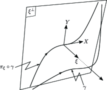
Figure 2.1: Orientations of $\xi^{\perp}$ and $\pi_{\xi}\circ\gamma$.

Suppose that we are given the information of the curvatures of the contours from two distinct directions $0<\theta_{1},\theta_{2}<\pi$ ($\theta_{1}\neq\theta_{2}$). Set $\varphi=\theta_{1}-\theta_{2}$ and $\tilde{\kappa}_{\theta_{j}}=(d\kappa_{\theta_{j}}/ds_{j}(0))^{1/3}$. We can determine the local information of space curves from local information of projected curves in two distinct directions:

Theorem 2.1.

If $(d\kappa_{\theta_{1}}/ds_{1}(0),d\kappa_{\theta_{2}}/ds_{2}(0))\neq(0,0)$, then the following hold.

1. $\theta_{1},\theta_{2}$ and $b_{3}$ are uniquely determined from the second order information of $\kappa_{\theta_{1}},\kappa_{\theta_{2}}$ at $0$ and $\varphi=\theta_{1}-\theta_{2}$.

2. The coefficients $a_{n-2}$ and $b_{n}$ are uniquely determined from the $(n-1)$-st order information of $\kappa_{\theta_{1}},\kappa_{\theta_{2}}$ at $0$ and $\varphi$ for $n\geq 4$.

The explicit formulae for $\theta_{1},\theta_{2}=\theta_{1}+\varphi$ and $b_{3}$ are given as in (2.6) and (2.9) in the proof.

Proof.

Let $e_{1},e_{2}$ be an orthonormal basis of the osculating plane of $\gamma$ at $0$. Then the curvature $\kappa_{\theta_{i}}$ for a general parameter $t$ is

$$\kappa_{\theta_{i}}(t)=\dfrac{\det\left({\begin{pmatrix}\gamma^{\prime}(t)\cdot e_{1}\\ \gamma^{\prime}(t)\cdot e_{2}\end{pmatrix}},{\begin{pmatrix}\gamma^{\prime\prime}(t)\cdot e_{1}\\ \gamma^{\prime\prime}(t)\cdot e_{2}\end{pmatrix}}\right)}{((\gamma^{\prime}(t)\cdot e_{1})^{2}+(\gamma^{\prime}(t)\cdot e_{2})^{2})^{3/2}}=\dfrac{\det\big{(}\gamma^{\prime}(t),\gamma^{\prime\prime}(t),\xi_{\theta_{i}}\big{)}}{|\gamma_{\theta_{i}}^{\prime}(t)|^{3}}\ \left({}^{\prime}=\dfrac{d}{dt}\right).$$

We set $\alpha(t)=\det\big{(}\gamma^{\prime}(t),\gamma^{\prime\prime}(t),\xi_{\theta_{i}}\big{)}$ and $\beta(t)=\gamma_{\theta_{i}}^{\prime}(t)\cdot\gamma_{\theta_{i}}^{\prime}(t)$. Then noticing $\alpha(0)=0$, we have

$$\kappa_{\theta_{i}}^{\prime}(0)= \alpha^{\prime}(0)/\beta(0)^{3/2}$$

$$\kappa_{\theta_{i}}^{\prime\prime}(0)= (-3\alpha^{\prime}(0)\beta^{\prime}(0)+\beta(0)\alpha^{\prime\prime}(0))/\beta(0)^{5/2}$$ (2.1)

$$\kappa_{\theta_{i}}^{\prime\prime\prime}(0)= \dfrac{1}{4\beta(0)^{7/2}}\Big{(}9\alpha^{\prime}(0)(5\beta^{\prime}(0)^{2}-2\beta(0)\beta^{\prime\prime}(0))$$

$$-18\alpha^{\prime\prime}(0)\beta(0)\beta^{\prime}(0)+4\alpha^{\prime\prime\prime}(0)\beta(0)^{2}\Big{)}$$

and

$$\alpha^{\prime}(0)= \det(\gamma^{\prime}(0),\gamma^{\prime\prime\prime}(0),\xi_{\theta_{i}})$$

$$\alpha^{\prime\prime}(0)= \det(\gamma^{\prime\prime}(0),\gamma^{\prime\prime\prime}(0),\xi_{\theta_{i}})+\det(\gamma^{\prime}(0),\gamma^{(4)}(0),\xi_{\theta_{i}})$$ (2.2)

$$\alpha^{\prime\prime\prime}(0)= 2\det(\gamma^{\prime\prime}(0),\gamma^{(4)}(0),\xi_{\theta_{i}})+\det(\gamma^{\prime}(0),\gamma^{(5)}(0),\xi_{\theta_{i}}).$$

Since $0<\theta_{i}<\pi$, it holds that $\sin\theta_{i}\neq 0$, and by a direct calculation we have

$$\operatorname{coef}(\kappa_{\theta_{i}},t,3)$$ (2.3)

$$= \Bigg{(}0,-\dfrac{b_{3}}{\sin^{2}\theta_{i}},-\dfrac{b_{4}\sin\theta_{i}+5a_{2}b_{3}\cos\theta_{i}}{2\sin^{3}\theta_{i}},$$

$$-\dfrac{1}{6\sin^{4}\theta_{i}}\Big{(}b_{5}\sin^{2}\theta_{i}$$

$$+(9a_{3}b_{3}+7a_{2}b_{4})\cos\theta_{i}\sin\theta_{i}+27a_{2}^{2}b_{3}\cos^{2}\theta_{i}\Big{)}\bigg{)}$$

for $i=1,2$. Since $s_{i}$ is an arc-length parameter of $\gamma_{\theta_{i}}$,

$$s_{i}(t)=\int^{t}_{0}\beta(t)^{1/2}\,dt.$$

We set $t(s_{i})$ to be the inverse function of the above $s_{i}(t)$. Then since $s_{i}^{\prime}(t)=\beta(t)^{1/2}$, we see that

$$\dfrac{dt}{ds_{i}}(s_{i}(t))= \dfrac{1}{s_{i}^{\prime}(t)}=\dfrac{1}{\beta(t)^{1/2}},$$

$$\dfrac{d^{2}t}{ds_{i}^{2}}(s_{i}(t))= -\dfrac{s_{i}^{\prime\prime}(t)}{(s_{i}^{\prime}(t))^{3}}=-\dfrac{\beta^{\prime}(t)}{2\beta(t)^{2}},$$

$$\dfrac{d^{3}t}{ds_{i}^{3}}(s_{i}(t))= \dfrac{3(s_{i}^{\prime\prime}(t))^{2}-s_{i}^{\prime}(t)s_{i}^{\prime\prime\prime}(t)}{(s_{i}^{\prime}(t))^{5}}=\dfrac{2(\beta^{\prime}(t))^{2}-\beta(t)\beta^{\prime\prime}(t)}{2\beta^{7/2}(t)}.$$

On the other hand, by the definition of $\beta$,

$$\operatorname{coef}(\beta,t,2)=\big{(}\sin^{2}\theta_{i},-2a_{2}\sin\theta_{i}\cos\theta_{i},\cos\theta_{i}(a_{2}^{2}\cos\theta_{i}-a_{3}\sin\theta_{i})\big{)}$$

holds. Thus

$$\operatorname{coef}\left(t(s_{i}),s_{i},3\right)=\bigg{(}0,\dfrac{1}{\sin\theta_{i}},\dfrac{a_{2}\cos\theta_{i}}{2\sin^{3}\theta_{i}},$$ (2.4)

$$\hskip 14.22636pt\dfrac{\cos\theta_{i}}{6\sin^{5}\theta_{i}}(3a_{2}^{2}\cos\theta_{i}+a_{3}\sin\theta_{i})\bigg{)}.$$

Moreover, by

$$\dfrac{d\kappa_{\theta_{i}}}{ds_{i}}(s_{i}) =\kappa_{1}^{\prime}(t(s_{i}))\dfrac{dt}{ds_{i}}(s_{i})$$

$$\dfrac{d^{2}\kappa_{\theta_{i}}}{ds_{i}^{2}}(s_{i}) =\kappa_{1}^{\prime\prime}(t(s_{i}))\left(\dfrac{dt}{ds_{i}}(s_{i})\right)^{2}+\kappa_{1}^{\prime}(t(s_{i}))\dfrac{dt^{2}}{d^{2}s_{i}}(s_{i})$$

$$\dfrac{d^{3}\kappa_{\theta_{i}}}{ds_{i}^{3}}(s_{i}) =\kappa_{1}^{\prime\prime\prime}(t(s_{i}))\left(\dfrac{dt}{ds_{i}}(s_{i})\right)^{3}+3\kappa_{1}^{\prime\prime}(t(s_{i}))\dfrac{dt}{ds_{i}}(s_{i})\dfrac{dt^{2}}{d^{2}s_{i}}(s_{i})$$

$$\hskip 28.45274pt+\kappa_{1}^{\prime}(t(s_{i}))\dfrac{dt^{3}}{d^{3}s_{i}}(s_{i})$$

together with (2.1), (2.2), (2.3) and (2.4), we have

$$\operatorname{coef}(\kappa_{\theta_{i}},s_{i},3)$$ (2.5)

$$= \Bigg{(}0,-\dfrac{b_{3}}{\sin^{3}\theta_{i}},-\dfrac{b_{4}\sin\theta_{i}+6a_{2}b_{3}\cos\theta_{i}}{2\sin^{5}\theta_{i}},$$

$$-\dfrac{1}{6\sin^{7}\theta_{i}}\Big{(}45a_{2}^{2}b_{3}\cos^{2}\theta_{i}+b_{5}\sin^{2}\theta_{i}$$

$$\hskip 14.22636pt+10(a_{3}b_{3}+a_{2}b_{4})\sin\theta_{i}\cos\theta_{i}\Big{)}\Bigg{)}.$$

By (2.5), the condition $d\kappa_{\theta_{1}}/ds_{1}(0)\neq 0$ or $d\kappa_{\theta_{2}}/ds_{2}(0)\neq 0$ implies $b_{3}\neq 0$. Thus $(d\kappa_{\theta_{1}}/ds_{1}(0),d\kappa_{\theta_{2}}/ds_{2}(0))\neq(0,0)$ implies $d\kappa_{\theta_{1}}/ds_{1}(0)\neq 0$ and $d\kappa_{\theta_{2}}/ds_{2}(0)\neq 0$. Taking another direction $\theta_{2}=\theta_{1}+\varphi$ $(0<\theta_{2}<\pi)$, we may consider $\kappa_{\theta_{1}},\kappa_{\theta_{2}},\varphi$ to be known. Since the equation

$$\dfrac{d\kappa_{\theta_{1}}/ds_{1}(0)}{d\kappa_{\theta_{2}}/ds_{2}(0)}=\dfrac{\sin^{3}(\theta_{1}+\varphi)}{\sin^{3}\theta_{1}}$$

can be solved as

$$\theta_{1}=\cot^{-1}\left(\dfrac{\left(\dfrac{d\kappa_{\theta_{1}}/ds_{1}(0)}{d\kappa_{\theta_{2}}/ds_{2}(0)}\right)^{1/3}-\cos\varphi}{\sin\varphi}\right)\in(0,\pi),$$ (2.6)

we obtain $\theta_{1}$ and $\theta_{2}$.

Furthermore, by (2.5), it holds that

$$\sin\theta_{i}=-\frac{\tilde{b}}{\tilde{\kappa}_{\theta_{i}}},\quad(i=1,2)$$ (2.7)

where $\tilde{b}=b_{3}^{1/3}$ and $\tilde{\kappa}_{\theta_{i}}=(d\kappa_{\theta_{i}}/ds_{i}(0))^{1/3}$. Substituting (2.7) into the trigonometric identity

$$\cos^{2}{(\theta_{1}-\theta_{2})}+\sin^{2}{\theta_{1}}+\sin^{2}{\theta_{2}}-2\sin{\theta_{1}}\sin{\theta_{2}}\cos{(\theta_{1}-\theta_{2})}-1=0,$$

we have

$$(\tilde{\kappa}_{\theta_{1}}^{2}-2\cos{\varphi}\;\tilde{\kappa}_{\theta_{1}}\tilde{\kappa}_{\theta_{2}}+\tilde{\kappa}_{\theta_{2}}^{2})\tilde{b}^{2}-\sin^{2}{\varphi}\;\tilde{\kappa}_{\theta_{1}}^{2}\tilde{\kappa}_{\theta_{2}}^{2}=0.$$ (2.8)

Since $\theta_{1}\neq\theta_{2}$, it holds that $\sin\varphi\neq 0$. Thus by $\tilde{\kappa}_{\theta_{1}}\tilde{\kappa}_{\theta_{2}}\neq 0$, we see that the equality (2.8) implies $\tilde{\kappa}_{\theta_{1}}^{2}-2\cos{\varphi}\;\tilde{\kappa}_{\theta_{1}}\tilde{\kappa}_{\theta_{2}}+\tilde{\kappa}_{\theta_{2}}^{2}\neq 0$. Thus (2.8) also implies that we obtain $b_{3}$, since $\tilde{\kappa}_{\theta_{1}}$, $\tilde{\kappa}_{\theta_{2}}$, $\varphi$ are known. In fact,

$$b_{3}=\left(\dfrac{\sin^{2}{\varphi}\;\tilde{\kappa}_{\theta_{1}}^{2}\tilde{\kappa}_{\theta_{2}}^{2}}{\tilde{\kappa}_{\theta_{1}}^{2}-2\cos{\varphi}\;\tilde{\kappa}_{\theta_{1}}\tilde{\kappa}_{\theta_{2}}+\tilde{\kappa}_{\theta_{2}}^{2}}\right)^{3/2},\quad\left(\tilde{\kappa}_{\theta_{i}}=\left(\dfrac{d\kappa_{\theta_{i}}}{ds_{i}}(0)\right)^{1/3}\quad(i=1,2)\right).$$ (2.9)

Thus the claim (1) holds.

Since the pair of equations

$$\dfrac{d^{2}\kappa_{\theta_{i}}}{ds_{i}^{2}}(0)=-\dfrac{b_{4}\sin\theta_{i}+6a_{2}b_{3}\cos\theta_{i}}{2\sin^{5}\theta_{i}}\quad(i=1,2)$$

is a linear system for $a_{2},b_{4}$, by $\theta_{1}\neq\theta_{2}$ we obtain $a_{2}$ and $b_{4}$ from (2.5) if $b_{3}\neq 0$. Thus the claim (2) when $n=4$ holds. Next, we show (2) when $n\geq 5$. We assume that $\varphi$, $a_{1},\ldots,a_{n-3}$ and $b_{1},\ldots,b_{n-1}$ are known for $n\geq 5$. Now we take the $(n-2)$-th derivative of $\kappa_{\theta_{i}}$ with respect to $s_{i}$. That value of the derivative at $0$ is written in terms of $a_{1},\ldots,a_{n}$ and $b_{1},\ldots,b_{n}$. In the formula of $d^{n-2}d\kappa_{\theta_{i}}/ds_{i}^{n-2}(0)$, as a polynomial of $a_{1},\ldots,a_{n},b_{1},\ldots,b_{n}$, we show that $a_{n-1},a_{n}$ do not appear, and $a_{n-2},b_{n}$ appear only to the first power linear terms. We set $\kappa_{\theta_{i}}=\kappa$ and $s_{i}=s$ for simplicity, for the moment. Let $t(s)$ be the inverse function of

$$s=\int_{0}^{t}|\gamma_{\theta_{i}}^{\prime}(t)|\,dt,$$

where ${}^{\prime}=d/dt$. By the formula for differentiation of a composition of functions (see [18, ($3_{n}$)] or [11, (3.56)] for example),

$$\dfrac{d^{n-2}}{ds^{n-2}}\kappa(t(s))=\sum_{k=0}^{n-2}\dfrac{d^{k}\kappa}{dt^{k}}(t(s))\dfrac{(-1)^{k}}{k!}\sum_{j=0}^{k}(-1)^{j}{\begin{pmatrix}k\\ j\end{pmatrix}}t(s)^{k-j}\dfrac{d^{n-2}}{ds^{n-2}}(t(s)^{j}),$$ (2.10)

and we look at the terms

$$\dfrac{d^{j}t(s)}{ds^{j}}(0),\quad\dfrac{d^{j}\kappa}{dt^{j}}(0),\quad(j=n-4,n-3,n-2).$$

Since $dt/ds=|\gamma_{\theta_{i}}^{\prime}|^{-1}$, it holds that

$$\dfrac{d^{j}t}{ds^{j}} =\dfrac{d^{j-1}}{ds^{j-1}}\left(\dfrac{1}{|\gamma_{\theta_{i}}^{\prime}(t(s))|}\right)=\dfrac{d^{j-1}}{ds^{j-1}}\left(\left\langle{\gamma_{\theta_{i}}^{\prime}(t(s))},{\gamma_{\theta_{i}}^{\prime}(t(s))}\right\rangle^{-1/2}\right)$$

$$=-\dfrac{d^{j-2}}{ds^{j-2}}\left(\left\langle{\gamma_{\theta_{i}}^{\prime}(t(s))},{\gamma_{\theta_{i}}^{\prime}(t(s))}\right\rangle^{-3/2}\left\langle{\gamma_{\theta_{i}}^{\prime}(t(s))},{\gamma_{\theta_{i}}^{\prime\prime}(t(s))}\right\rangle\dfrac{dt(s)}{ds}\right)$$

$$=-\dfrac{d^{j-2}}{ds^{j-2}}\left(\left\langle{\gamma_{\theta_{i}}^{\prime}(t(s))},{\gamma_{\theta_{i}}^{\prime}(t(s))}\right\rangle^{-2}\left\langle{\gamma_{\theta_{i}}^{\prime}(t(s))},{\gamma_{\theta_{i}}^{\prime\prime}(t(s))}\right\rangle\right).$$

Continuing to calculate the derivative of the function by $s$, we finally obtain a polynomial consisting of terms with some powers of $\left\langle{\gamma_{\theta_{i}}^{\prime}(t(s))},{\gamma_{\theta_{i}}^{\prime}(t(s))}\right\rangle$ and

$$\left\langle{\gamma_{\theta_{i}}^{(\ell_{1})}(t(s))},{\gamma_{\theta_{i}}^{(\ell_{2})}(t(s))}\right\rangle\quad(1\leq\ell_{1}\leq\ell_{2}\leq j,\ 3\leq\ell_{1}+\ell_{2}\leq j+1).$$

This implies that $a_{n-1},a_{n},b_{n}$ do not appear in $(d^{j}t(s)/ds^{j})(0)$ $(j=n-4,n-3,n-2)$. Moreover, although $a_{n-2}$ may appear in $(d^{n-2}t(s)/ds^{n-2})(0)$ from the term $\langle\gamma_{\theta_{i}}^{\prime},\gamma_{\theta_{i}}^{(n-2)}\rangle,$ it does not actually appear, since $\gamma_{\theta_{i}}^{\prime}(0)=(1,0,0)$ and the first component of $\gamma_{\theta_{i}}^{(n-2)}(0)$ is $0$. On the other hand, since $\gamma$ is given by (1.1),

$$\begin{split}\det(\gamma^{\prime},\gamma^{(n-2)},\xi_{\theta_{i}})=&-b_{n-2}\sin\theta_{i},\ \det(\gamma^{\prime},\gamma^{(n-1)},\xi_{\theta_{i}})=-b_{n-1}\sin\theta_{i},\\ \det(\gamma^{\prime},\gamma^{(n)},\xi_{\theta_{i}})=&-\boxed{b_{n}}\sin\theta_{i},\\ \det(\gamma^{\prime\prime},\gamma^{(n-2)},\xi_{\theta_{i}})=&a_{2}b_{n-2}\cos\theta_{i},\ \det(\gamma^{\prime\prime},\gamma^{(n-1)},\xi_{\theta_{i}})=a_{2}b_{n-1}\cos\theta_{i},\\ \det(\gamma^{\prime\prime\prime},\gamma^{(n-2)},\xi_{\theta_{i}})=&(a_{3}b_{n-2}-b_{3}\boxed{a_{n-2}})\cos\theta_{i},\end{split}$$ (2.11)

and $a_{n-2},a_{n-1},a_{n},b_{n}$ do not appear in $\det(\gamma^{\prime},\gamma^{\prime\prime},\xi_{\theta_{i}})^{(j)}(0)$ $(j=1,\ldots,n-3)$. This implies that they also do not appear in $d^{j}\kappa/dt^{j}$ $(j=1,\ldots,n-3)$. Furthermore, since

$$\begin{split}\dfrac{d^{n-2}\kappa}{dt^{n-2}}=&\sum_{j+k\leq n}c_{jk}\left(\dfrac{1}{|\gamma^{\prime}_{\theta_{i}}|^{3}}\right)^{(n-2-j-k)}\det(\gamma^{(j)},\gamma^{(k)},\xi_{\theta_{i}})\\ &\hskip 28.45274pt+\dfrac{1}{|\gamma^{\prime}_{\theta_{i}}|^{3}}\bigg{(}\det(\gamma^{\prime},\gamma^{(n)},\xi_{\theta_{i}})+(n-3)\det(\gamma^{\prime\prime},\gamma^{(n-1)},\xi_{\theta_{i}})\\ &\hskip 85.35826pt+m\det(\gamma^{\prime\prime\prime},\gamma^{(n-2)},\xi_{\theta_{i}})\bigg{)}\end{split}$$ (2.12)

$(n\geq 5)$ holds, where $m=(n-5)(n-2)/2$ and $c_{jk}$ are natural numbers, this implies that $a_{n-1},a_{n}$ do not appear in (2.10). Moreover, since the coefficient of $d^{n-2}\kappa/dt^{n-2}$ in (2.10) is $(dt/ds)^{n-2}$, setting

$$A_{i}=\dfrac{1}{|\gamma^{\prime}_{\theta_{i}}(0)|^{3}}\left(\dfrac{dt}{ds}(0)\right)^{n-2},$$

the equations (2.10) at $s=0$ for $i=1,2$ are

$$\begin{split}\dfrac{d^{n-2}\kappa_{\theta_{1}}}{ds_{1}^{n-2}}(0)=-A_{1}(b_{n}\sin\theta_{1}+mb_{3}a_{n-2}\cos\theta_{1})+B_{1},\\ \dfrac{d^{n-2}\kappa_{\theta_{2}}}{ds_{2}^{n-2}}(0)=-A_{2}(b_{n}\sin\theta_{2}+mb_{3}a_{n-2}\cos\theta_{2})+B_{2},\end{split}$$ (2.13)

where $B_{i}$ $(i=1,2)$ are terms consisting of $a_{1},\ldots,a_{n-3}$ and $b_{1},\ldots,b_{n-1}$. The equation (2.13) can be solved when $A_{1}A_{2}b_{3}\sin(\theta_{1}-\theta_{2})\neq 0$. Since $dt/ds(0)=|\gamma_{\theta_{i}}^{\prime}(0)|^{-1}$, we have the assertion. ∎

Since obtaining $a_{2},a_{3},b_{3}$ is equivalent to obtaining the curvature, the first derivative of the curvature and the torsion, results of this type for the perspective projection can be found in [3, 17] and [7, Theorem 8]. Since we can detect the coefficients of the Taylor expansion of $\gamma$, using our result, one can easily construct the desired curve whose projections have the prescribed curvatures.

2.2 Projections in the tangential direction and another direction

In this section, we consider the case that $\xi_{1}$ is tangent to $\gamma$ at $0$. In this case, $\gamma_{\xi_{1}}=\pi_{\xi_{1}}\circ\gamma$ has a singular point at $0$. To consider differential geometric invariants of the singular curve, we describe the cuspidal curvature of singular plane curves introduced in [20] (see also [21]). Let $c:I\to\boldsymbol{R}^{2}$ be a plane curve, and $c^{\prime}(0)=0$. The curve $c$ is said to be $A$-type at $0$ if $c^{\prime\prime}(0)\neq 0$. Let $c$ be an $A$-type curve at $0$. Then

$$\mu=\dfrac{\det(c^{\prime\prime}(0),c^{\prime\prime\prime}(0))}{|c^{\prime\prime}(0)|^{5/2}}.$$

does not depend on the choice of parameter, and is called the cuspidal curvature.

Let $\gamma:I\to\boldsymbol{R}^{3}$ be a $C^{\infty}$ curve with non-zero curvature at $0$. We assume that $\gamma_{\xi_{1}}$ has a singular point at $0$. Since the curvature of $\gamma$ does not vanish, by the Frenet formula, $\gamma_{\xi_{1}}(0)$ is an $A$-type curve at $0$. We also assume that there exists an integer $N$ such that $\det((\gamma_{\xi_{1}})^{\prime\prime},(\gamma_{\xi_{1}})^{(i)})(0)=0$ ($i=3,5,\ldots,2N-1$) and $\det((\gamma_{\xi_{1}})^{\prime\prime},(\gamma_{\xi_{1}})^{(2N+1)})(0)\neq 0$. We give the positively oriented $xyz$-coordinate system for $\boldsymbol{R}^{3}$, and rotating this coordinate system, we give a $yz$-coordinate system for $\xi_{1}^{\perp}$ as follows. We set the $y$-axis as the direction of $(\gamma_{\xi_{1}})^{\prime\prime}(0)$, and set the $x$-axis as the direction of $\xi_{1}$. We give an orientation of $\gamma_{\xi_{1}}$ so that $\det((\gamma_{\xi_{1}})^{\prime\prime},(\gamma_{\xi_{1}})^{(2N+1)})(0)>0$, and also that of $\gamma$ agrees with that of $\gamma_{\xi_{1}}$ (see Figure 2.2). Then we may assume that $\gamma$ is given by (1.1) with $a_{2}>0,b_{3}\geq 0$. Then $\mu=b_{3}/a_{2}^{3/2}$. On the other hand, we consider a unit vector $\xi_{2}=(\sin\theta_{1}\cos\theta_{2},\sin\theta_{1}\sin\theta_{2},\cos\theta_{1})$ $(\cos\theta_{1}\neq 0)$ which is not tangent to $\gamma$ at $0$. Since we take the above $xyz$-coordinate, $\theta_{1},\theta_{2}$ are known.

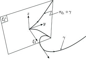
Figure 2.2: Orientations of $\xi_{1}^{\perp}$ and $\pi_{\xi_{1}}\circ\gamma$.

Theorem 2.2.

Suppose that $\cos\theta_{1}\neq 0$, then the following hold.

1. The coefficients $a_{2}$ and $b_{3}$ are uniquely determined by the cuspidal curvature $\mu$ and the $0$-th order information of $\kappa_{\xi_{2}}$ at $0$.

2. In addition to (1), $a_{3}$ is uniquely determined by the cuspidal curvature $\mu$ and the first order information of $\kappa_{\xi_{2}}$ at $0$.

Proof.

We remark that $\cos\theta_{1}\neq 0$ implies $\cos^{2}\theta_{1}\cos^{2}\theta_{2}+\sin^{2}\theta_{2}\neq 0$. The curvature $\kappa_{\xi_{2}}$ of the plane curve $\gamma_{\xi_{2}}$ satisfies

$$\operatorname{coef}(\kappa_{\xi_{2}},s,1)= \Bigg{(}\dfrac{a_{2}\cos\theta_{1}}{(\cos^{2}\theta_{1}\cos^{2}\theta_{2}+\sin^{2}\theta_{2})^{3/2}},\;\;\dfrac{Q(\theta)}{(\cos^{2}\theta_{1}\cos^{2}\theta_{2}+\sin^{2}\theta_{2})^{3}}\Bigg{)},$$ (2.14)

where

$$Q(\theta)=-b_{3}\cos^{2}\theta_{1}\cos^{2}\theta_{2}\sin\theta_{1}\sin\theta_{2}-b_{3}\sin\theta_{1}\sin^{3}\theta_{2}$$

$$\hskip 14.22636pt+\cos^{3}\theta_{1}\cos\theta_{2}(a_{3}\cos\theta_{2}-3a_{2}^{2}\sin\theta_{2})+\cos\theta_{1}\sin\theta_{2}(3a_{2}^{2}\cos\theta_{2}+a_{3}\sin\theta_{2}).$$

Since we know $\mu=b_{3}/a_{2}^{3/2}$ and $\theta_{1},\theta_{2}$, we obtain $a_{2}$ and $b_{3}$ from the first component of (2.14) if $\cos\theta_{1}\neq 0$. Furthermore, we also obtain $a_{3}$ from the second component of (2.14), under the assumption $\cos\theta_{1}(\cos^{2}\theta_{1}\cos^{2}\theta_{2}+\sin^{2}\theta_{2})\neq 0$. ∎

See [16, Section 3] for relationships between invariants of space curves and projected plane curves.

3 Projections of surfaces

In this section, we consider the local information of surfaces and contours. Let $U\subset\boldsymbol{R}^{2}$ be a neighborhood of the origin $0=(0,0)$. Let $f:U\to\boldsymbol{R}^{3}$ ($f(0)=(0,0,0)$) be a $C^{\infty}$ surface with non-vanishing Gaussian curvature at $0$. We assume that $0$ is not an umbilical point. Without loss of generality, we may assume that $f$ is written in the form (1.2) with $a_{20}a_{02}\neq 0$, $a_{20}>a_{02}$, $a_{20}>0$. We set the unit normal vector $\nu$ of $f$ so that it satisfies $\nu(0,0)=(0,0,1)$.

3.1 Obtaining information about surfaces from contours

Let $\xi$ be a unit vector which is tangent to $f$ at $0$. Then we may assume $\xi=\xi(\theta_{1})=(\cos\theta_{1},\sin\theta_{1},0)$, where $0<\theta_{1}<\pi$. The set $S$ of singular points of the map $\pi_{\xi(\theta_{1})}\circ f$ is

$$S=\{(u,v)\,|\,\cos\theta_{1}h_{u}+\sin\theta_{1}h_{v}=0\},$$ (3.1)

where $h$ is given in (1.2). We assume

$$p(\theta_{1})=a_{20}\cos^{2}\theta_{1}+a_{02}\sin^{2}\theta_{1}\neq 0,$$

which implies that the direction $\xi(\theta_{1})$ is not an asymptotic direction of $f$ at the origin. By the assumption $a_{02}\neq 0$ and $0<\theta_{1}<\pi$, it holds that

$$(\cos\theta_{1}h_{u}+\sin\theta_{1}h_{v})_{v}(0,0)=a_{02}\sin\theta_{1}\neq 0,$$

and this implies that there exists a regular parametrization of $S$. For the purpose of taking this parametrization, we set an orientation of $S$ as follows. First, we give an orientation of the normal plane $\xi(\theta_{1})^{\perp}$ of $\xi(\theta_{1})$ such that

$$X=(-\sin\theta_{1},\cos\theta_{1},0),\quad Y=(0,0,1)$$

is a positive basis. Next, we put an orientation on $(\pi_{\xi(\theta_{1})}\circ f)(S)$ so that it agrees with the direction of $X$, and also put that of $S$ agreeing with $(\pi_{\xi(\theta_{1})}\circ f)(S)$ (see Figure 3.1).

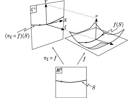
Figure 3.1: Orientations of $\xi^{\perp}$ and the contour.

Let $k_{\theta}$ be the curvature of the contour from a direction $\theta$.

Lemma 3.1.

The first order information $k_{\theta}$ with respect to the arc-length parameter $s$ $($suitably oriented$)$ are

$$\operatorname{coef}(k_{\theta_{1}},1,s)=\Bigg{(}\dfrac{a_{20}a_{02}}{p(\theta_{1})},\dfrac{q(\theta_{1})}{p(\theta_{1})^{3}}\Bigg{)},$$ (3.2)

where

$$q(\theta_{1}) =a_{03}a_{20}^{3}\cos^{3}\theta_{1}-3a_{02}a_{12}a_{20}^{2}\cos^{2}\theta_{1}\sin\theta_{1}$$

$$\hskip 28.45274pt+3a_{02}^{2}a_{20}a_{21}\cos\theta_{1}\sin^{2}\theta_{1}-a_{02}^{3}a_{30}\sin^{3}\theta_{1}.$$ (3.3)

Proof.

Since $a_{02}\sin\theta_{1}\neq 0$, we can take a parametrization $C(t)=(t,c(t))$ of $S$. Then since $\pi_{\xi(\theta_{1})}\circ f\circ C$ lies on the plane $\xi(\theta_{1})^{\perp}$,

$$k_{\theta_{1}}(0)= \dfrac{\det\big{(}\hat{C}^{\prime},\hat{C}^{\prime\prime},\xi(\theta_{1})\big{)}}{|\hat{C}^{\prime}|^{3}}(0),$$

$$\dfrac{dk_{\theta_{1}}}{ds}(0)= \dfrac{\det\big{(}\hat{C}^{\prime},\hat{C}^{\prime\prime\prime},\xi(\theta_{1})\big{)}}{|\hat{C}^{\prime}|^{4}}(0)+3\left\langle{\hat{C}^{\prime}},{\hat{C}^{\prime\prime}}\right\rangle(0)\dfrac{\det\big{(}\hat{C}^{\prime},\hat{C}^{\prime\prime},\xi(\theta_{1})\big{)}}{|\hat{C}^{\prime}|^{6}}(0)$$

where $\hat{C}=f\circ C=f(t,c(t))$ and ${}^{\prime}=d/dt$. Since $h^{\prime}(t,c(t))=0$ at $t=0$, it holds that

$$\det\big{(}\hat{C}^{\prime},\hat{C}^{(i)},\xi(\theta_{1})\big{)}=(c^{\prime}\cos\theta_{1}+\sin\theta_{1})(h\circ C)^{(i)}\quad(i=2,3),$$

where $\hat{C}^{(2)}=\hat{C}^{\prime\prime}$ and $\hat{C}^{(3)}=\hat{C}^{\prime\prime\prime}$. By (3.1), it holds that

$$\operatorname{coef}(c(t),2,t)= \Bigg{(}0,\;\;-\dfrac{a_{20}\cos\theta_{1}}{a_{02}\sin\theta_{1}},\;\;\dfrac{1}{a_{02}^{3}\sin^{3}\theta_{1}}\tilde{q}(\theta_{1})\Bigg{)},$$

where

$$\tilde{q}(\theta_{1})= -a_{12}a_{20}^{2}\cos^{3}\theta_{1}-a_{03}a_{20}^{2}\cos^{2}\theta_{1}\sin\theta_{1}+2a_{02}a_{20}a_{21}\cos^{2}\theta_{1}\sin\theta_{1}$$

$$+ 2a_{02}a_{12}a_{20}\cos\theta_{1}\sin^{2}\theta_{1}-a_{02}^{2}a_{30}\cos\theta_{1}\sin^{2}\theta_{1}-a_{02}^{2}a_{21}\sin^{3}\theta_{1}.$$

Summarizing up the above calculation, we have the assertion. ∎

The inner product of $(\pi_{\xi(\theta_{1})}\circ f\circ C)^{\prime}(0)$ and $X$ is

$$\left\langle{(\pi_{\xi(\theta_{1})}\circ f\circ C)^{\prime}(0)},{X}\right\rangle=\dfrac{-1}{a_{02}\sin\theta_{1}}p(\theta_{1}).$$ (3.4)

Let $s$ be the arc-length parameter of $S$ where the orientation is given in the above manner. Thus we remark that by (3.4), if $a_{02}\sin\theta_{1}p(\theta_{1})$ is negative, $s$ is the opposite direction to the above parameter $t$.

Remark 3.2.

If $a_{20}a_{02}\neq 0$ and $p(\theta_{1})\neq 0$, then $q(\theta_{1})=0$ if and only if the contour has a vertex at $(\pi_{\xi(\theta_{1})}\circ f\circ C)(0)$, and $\xi(\theta_{1})=(\cos\theta_{1},\sin\theta_{1},0)$ is called the cylindrical direction of $f$ at the origin (see [9] for details).

Now we consider obtaining the second order information of the surface by the contours of the projections of three distinct directions. Let $f$ be the surface given by (1.2). Since the mean and the Gaussian curvatures of $f$ are $(a_{20}+a_{02})/2$ and $a_{20}a_{02}$ respectively, if the mean and the Gaussian curvatures are obtained, then one can conclude that the second order information are obtained. Thus we consider obtaining the mean and the Gaussian curvatures. We set $M$ and $G$ to be the mean and the Gaussian curvatures at $0$:

$$M=\frac{a_{20}+a_{02}}{2},\quad G=a_{20}a_{02}.$$ (3.5)

We also take another direction $\theta_{2}(\neq\theta_{1},0<\theta_{2}<\pi)$ which satisfies $p(\theta_{2})\neq 0$. By (3.2) we get

$$\cos 2\theta_{i}=\frac{-2a_{20}a_{02}+(a_{20}+a_{02})k_{\theta_{i}}}{(a_{02}-a_{20})k_{\theta_{i}}}\quad(i=1,2).$$ (3.6)

Substituting these formulae into the trigonometric identity

$$\cos^{2}2(\theta_{i}-\theta_{j})+\cos^{2}2\theta_{i}+\cos^{2}2\theta_{j}-2\cos 2(\theta_{i}-\theta_{j})\cos 2\theta_{i}\cos 2\theta_{j}-1=0,$$

$(i,j=1,2)$ we get an equation $P_{ij}(M,G)=0$ where

$$P_{ij}(M,G)= \left(M_{ij}^{2}-G_{ij}\cos^{2}(\theta_{i}-\theta_{j})\right)G^{2}-2G_{ij}M_{ij}\sin^{2}(\theta_{i}-\theta_{j})GM$$

$$+G_{ij}^{2}\sin^{4}(\theta_{i}-\theta_{j})M^{2}+G_{ij}^{2}\cos^{2}(\theta_{i}-\theta_{j})\sin^{2}(\theta_{i}-\theta_{j})G$$

$$= (M,G)\;Q_{ij}\;{\begin{pmatrix}G\\ M\end{pmatrix}}+G_{ij}^{2}\cos^{2}(\theta_{i}-\theta_{j})\sin^{2}(\theta_{i}-\theta_{j})G$$ (3.7)

and

$$M_{ij}= \frac{k_{\theta_{i}}+k_{\theta_{j}}}{2},\ G_{ij}=k_{\theta_{i}}k_{\theta_{j}},$$ (3.8)

$$Q_{ij}= {\begin{pmatrix}M_{ij}^{2}-G_{ij}\cos^{2}(\theta_{i}-\theta_{j})&-G_{ij}M_{ij}\sin^{2}(\theta_{i}-\theta_{j})\\ -G_{ij}M_{ij}\sin^{2}(\theta_{i}-\theta_{j})&G_{ij}^{2}\sin^{4}(\theta_{i}-\theta_{j})\end{pmatrix}}.$$

Since $P_{ij}(M,G)=0$ is a quadratic curve, generally the values of $G$ and $M$ should be determined by the curvatures of the apparent contours from three distinct directions.

Theorem 3.3.

Take three distinct directions $0<\theta_{1},\theta_{2},\theta_{3}<\pi$ satisfying $p(\theta_{i})\not=0$ and $\sin 2\theta_{1}+\sin 2\theta_{2}+\sin 2\theta_{3}\neq 0$. Then $G$ and $M$ are given as follows:

$$G=\dfrac{\det L}{\det V},\quad M=\dfrac{\det P}{\det V},$$ (3.9)

where

$$x_{1}= {\vphantom{\left(\dfrac{M_{12}}{G_{12}},\dfrac{M_{23}}{G_{23}},\dfrac{M_{31}}{G_{31}}\right)}}^{t}{\!\left(\dfrac{M_{12}}{G_{12}},\dfrac{M_{23}}{G_{23}},\dfrac{M_{31}}{G_{31}}\right)},$$

$$x_{2}= {\vphantom{\left(\dfrac{M_{12}^{2}-G_{12}\cos^{2}(\theta_{1}-\theta_{2})}{G_{12}^{2}\sin^{2}(\theta_{1}-\theta_{2})},\dfrac{M_{23}^{2}-G_{23}\cos^{2}(\theta_{2}-\theta_{3})}{G_{23}^{2}\sin^{2}(\theta_{2}-\theta_{3})},\right.}}^{t}{\!\left(\dfrac{M_{12}^{2}-G_{12}\cos^{2}(\theta_{1}-\theta_{2})}{G_{12}^{2}\sin^{2}(\theta_{1}-\theta_{2})},\dfrac{M_{23}^{2}-G_{23}\cos^{2}(\theta_{2}-\theta_{3})}{G_{23}^{2}\sin^{2}(\theta_{2}-\theta_{3})},\right.}$$

$$\hskip 142.26378pt\left.\dfrac{M_{31}^{2}-G_{31}\cos^{2}(\theta_{3}-\theta_{1})}{G_{31}^{2}\sin^{2}(\theta_{3}-\theta_{1})}\right),$$

$$x_{3}= {\vphantom{\big{(}\cos^{2}(\theta_{1}-\theta_{2}),\cos^{2}(\theta_{2}-\theta_{3}),\cos^{2}(\theta_{3}-\theta_{1})\big{)}}}^{t}{\!\big{(}\cos^{2}(\theta_{1}-\theta_{2}),\cos^{2}(\theta_{2}-\theta_{3}),\cos^{2}(\theta_{3}-\theta_{1})\big{)}},$$ (3.10)

$$x_{4}= {\vphantom{\big{(}\sin^{2}(\theta_{1}-\theta_{2}),\sin^{2}(\theta_{2}-\theta_{3}),\sin^{2}(\theta_{3}-\theta_{1})\big{)}}}^{t}{\!\big{(}\sin^{2}(\theta_{1}-\theta_{2}),\sin^{2}(\theta_{2}-\theta_{3}),\sin^{2}(\theta_{3}-\theta_{1})\big{)}}$$ (3.11)

and

$$L=\big{(}x_{1},x_{3},x_{4}\big{)},\quad P=\big{(}x_{2},x_{3},x_{4}\big{)},\quad V=\big{(}x_{1},x_{2},x_{4}\big{)}.$$

Here ${\vphantom{(~{})}}^{t}{\!(~{})}$ stands for the transpose of a matrix.

Proof.

A triplet of the equations $P_{12}(M,G)=P_{23}(M,G)=P_{31}(M,G)=0$ is a system of equations

$$W{\begin{pmatrix}G^{2}\\ GM\\ M^{2}\end{pmatrix}}=Gb,$$

where $W=(w_{1},w_{2},w_{3})$ with

$$w_{1} ={\begin{pmatrix}M_{12}^{2}-G_{12}\cos^{2}(\theta_{1}-\theta_{2})\\ M_{23}^{2}-G_{23}\cos^{2}(\theta_{2}-\theta_{3})\\ M_{31}^{2}-G_{31}\cos^{2}(\theta_{3}-\theta_{1})\end{pmatrix}},$$ (3.12)

$$w_{2} =-{\begin{pmatrix}2G_{12}M_{12}\sin^{2}(\theta_{1}-\theta_{2})\\ 2G_{23}M_{23}\sin^{2}(\theta_{2}-\theta_{3})\\ 2G_{31}M_{31}\sin^{2}(\theta_{3}-\theta_{1})\end{pmatrix}},\ w_{3}={\begin{pmatrix}G_{12}^{2}\sin^{4}(\theta_{1}-\theta_{2})\\ G_{23}^{2}\sin^{4}(\theta_{2}-\theta_{3})\\ G_{31}^{2}\sin^{4}(\theta_{3}-\theta_{1})\end{pmatrix}},$$ (3.13)

and

$$b={\begin{pmatrix}G_{12}^{2}\cos^{2}(\theta_{1}-\theta_{2})\sin^{2}(\theta_{1}-\theta_{2})\\ G_{23}^{2}\cos^{2}(\theta_{2}-\theta_{3})\sin^{2}(\theta_{2}-\theta_{3})\\ G_{31}^{2}\cos^{2}(\theta_{3}-\theta_{1})\sin^{2}(\theta_{3}-\theta_{1})\end{pmatrix}}.$$ (3.14)

Since

$$\det W=-2G_{12}^{2}G_{23}^{2}G_{31}^{2}\sin^{2}(\theta_{1}-\theta_{2})\sin^{2}(\theta_{2}-\theta_{3})\sin^{2}(\theta_{3}-\theta_{1})\det V,$$

if $k_{\theta_{1}}k_{\theta_{2}}k_{\theta_{3}}\neq 0$, by Cramer’s rule, we get

$$G=\dfrac{\det W_{1}}{\det W},\ M=\dfrac{\det W_{2}}{\det W},\$$ (3.15)

where $W_{1}=(b,w_{2},w_{3})$, $W_{2}=(w_{1},b,w_{3})$. By a direct calculation, we have (3.9). Furthermore, since by (3.6), it holds that $k_{i}=2a_{20}a_{02}/\big{(}a_{20}+a_{02}+\cos 2\theta_{i}(a_{20}-a_{02})\big{)}$, we have

$$\det V= \dfrac{(a_{02}-a_{20})}{2a_{20}^{2}a_{02}^{2}}\Big{(}\sin(\theta_{1}-\theta_{2})\sin(\theta_{2}-\theta_{3})\sin(\theta_{3}-\theta_{1})$$

$$\hskip 113.81102pt\big{(}\sin 2\theta_{1}+\sin 2\theta_{2}+\sin 2\theta_{3}\big{)}\Big{)}.$$

Thus we have the condition $\sin 2\theta_{1}+\sin 2\theta_{2}+\sin 2\theta_{3}\neq 0$. ∎

Since in our setting, $\theta_{1}-\theta_{2}$, $\theta_{1}-\theta_{3}$, $k_{\theta_{1}}$, $k_{\theta_{2}}$, $k_{\theta_{3}}$ are known, all matrix elements of $W$ and $b$ are known. Thus we obtain $G$ and $M$ by (3.15). Moreover, we obtain $\theta_{1}$, $\theta_{2}$ and $\theta_{3}$ by (3.6). Since $G=a_{20}a_{02}$ and $M=(a_{20}+a_{02})/2$, we obtain $a_{20}$ and $a_{02}$. We remark that the set

$$\{(\theta_{1},\theta_{2},\theta_{3})\in(0,\pi)^{3}\,|\,\sin 2\theta_{1}+\sin 2\theta_{2}+\sin 2\theta_{3}\neq 0\}$$ (3.16)

is an open and dense subset of $(0,\pi)^{3}$. On the other hand, let us set $f_{1}(u,v)=(u,v,u^{2}+2v^{2})$ and $\theta_{1}=0,\theta_{2}=\pi/6,\theta_{3}=-\pi/6$. Then $\sin 2\theta_{1}+\sin 2\theta_{2}+\sin 2\theta_{3}=0$. Let $\xi(\theta)=(\cos\theta,\sin\theta,0)$ be a unit vector and let $k^{1}_{\theta}$ be the curvature of the contour from the direction $\theta$ about $f_{1}$. Then

$$k^{1}_{\theta_{1}}=4,\quad k^{1}_{\theta_{2}}=k^{1}_{\theta_{3}}=\dfrac{50}{7\sqrt{7}}.$$

Let us set $f_{2}(u,v)=(u,v,au^{2}+2v^{2})$ and $\theta_{1}=0,\theta_{2}=\pi/4,\theta_{3}=-\pi/4$. Then $\sin 2\theta_{1}+\sin 2\theta_{2}+\sin 2\theta_{3}=0$ also holds. Let $k^{2}_{\theta}$ be the curvature of the contour from the direction $\theta$ about $f_{2}$. Then

$$k^{2}_{\theta_{1}}=4,\quad k^{2}_{\theta_{2}}=k^{2}_{\theta_{3}}=\dfrac{2\sqrt{2}a(2+a)^{2}}{(4+a^{2})^{3/2}},$$

and there is a solution $a$ of the equation

$$\dfrac{2\sqrt{2}a(2+a)^{2}}{(4+a^{2})^{3/2}}-\dfrac{50}{7\sqrt{7}}=0.$$ (3.17)

In fact, the left hand side of (3.17) is $2(441\sqrt{10}-625\sqrt{7})/1225<0$ when $a=1$, and it is $2(98-25\sqrt{7})/49>0$ when $a=2$. This implies that the condition $\sin 2\theta_{1}+\sin 2\theta_{2}+\sin 2\theta_{3}\neq 0$ cannot be removed from the condition of Theorem 3.3.

Next let us consider the third order terms of the surface. Let us take four distinct directions

$$\theta_{1},\ \theta_{2},\ \theta_{3},\ \theta_{4}.$$

Then we obtain $a_{30},a_{21},a_{12},a_{03}$ by $k_{\theta_{i}}$ $(i=1,2,3,4)$ as follows. By (3.2) and (3.3), we see that

$$A{\begin{pmatrix}a_{30}\\ a_{21}\\ a_{12}\\ a_{03}\end{pmatrix}}=d,$$

where $A=(a_{1},a_{2},a_{3},a_{4})$ and

$$a_{1} =-a_{02}^{3}{\vphantom{\Big{(}\sin^{3}\theta_{1},\ \sin^{3}\theta_{2},\ \sin^{3}\theta_{3},\ \sin^{3}\theta_{4}\Big{)}}}^{t}{\!\Big{(}\sin^{3}\theta_{1},\ \sin^{3}\theta_{2},\ \sin^{3}\theta_{3},\ \sin^{3}\theta_{4}\Big{)}},$$

$$a_{2} =3a_{20}a_{02}^{2}{\vphantom{\Big{(}\sin^{2}\theta_{1}\cos\theta_{1},\ \sin^{2}\theta_{2}\cos\theta_{2},\ \sin^{2}\theta_{3}\cos\theta_{3},\ \sin^{2}\theta_{4}\cos\theta_{4}\Big{)}}}^{t}{\!\Big{(}\sin^{2}\theta_{1}\cos\theta_{1},\ \sin^{2}\theta_{2}\cos\theta_{2},\ \sin^{2}\theta_{3}\cos\theta_{3},\ \sin^{2}\theta_{4}\cos\theta_{4}\Big{)}},$$

$$a_{3} =-3a_{20}^{2}a_{02}{\vphantom{\Big{(}\sin\theta_{1}\cos^{2}\theta_{1},\ \sin\theta_{2}\cos^{2}\theta_{2},\ \sin\theta_{3}\cos^{2}\theta_{3},\ \sin\theta_{4}\cos^{2}\theta_{4}\Big{)}}}^{t}{\!\Big{(}\sin\theta_{1}\cos^{2}\theta_{1},\ \sin\theta_{2}\cos^{2}\theta_{2},\ \sin\theta_{3}\cos^{2}\theta_{3},\ \sin\theta_{4}\cos^{2}\theta_{4}\Big{)}},$$

$$a_{4} =a_{20}^{3}{\vphantom{\Big{(}\cos^{3}\theta_{1},\ \cos^{3}\theta_{2},\ \cos^{3}\theta_{3},\ \cos^{3}\theta_{4}\Big{)}}}^{t}{\!\Big{(}\cos^{3}\theta_{1},\ \cos^{3}\theta_{2},\ \cos^{3}\theta_{3},\ \cos^{3}\theta_{4}\Big{)}},$$

$$d ={\vphantom{\Big{(}p(\theta_{1})^{3}\dfrac{dk_{\theta_{1}}}{ds}(0),\ p(\theta_{2})^{3}\dfrac{dk_{\theta_{2}}}{ds}(0),\ p(\theta_{3})^{3}\dfrac{dk_{\theta_{3}}}{ds}(0),\ p(\theta_{4})^{3}\dfrac{dk_{\theta_{4}}}{ds}(0)\Big{)}}}^{t}{\!\Big{(}p(\theta_{1})^{3}\dfrac{dk_{\theta_{1}}}{ds}(0),\ p(\theta_{2})^{3}\dfrac{dk_{\theta_{2}}}{ds}(0),\ p(\theta_{3})^{3}\dfrac{dk_{\theta_{3}}}{ds}(0),\ p(\theta_{4})^{3}\dfrac{dk_{\theta_{4}}}{ds}(0)\Big{)}}.$$

Since $\det A=9a_{20}^{6}a_{02}^{6}\prod_{i<j}\sin(\theta_{i}-\theta_{j})$, and $\theta_{1},\ldots,\theta_{4}$ are distinct, $a_{20}a_{02}\neq 0$, and it holds that $\det A\neq 0$. By Cramer’s rule, we get

$$a_{30}=\dfrac{\det A_{1}}{\det A},\ a_{21}=\dfrac{\det A_{2}}{\det A},\ a_{12}=\dfrac{\det A_{3}}{\det A},\ a_{03}=\dfrac{\det A_{4}}{\det A},$$ (3.18)

where $A_{1}=(d,a_{2},a_{3},a_{4})$, $A_{2}=(a_{1},d,a_{3},a_{4})$, $A_{3}=(a_{1},a_{2},d,a_{4})$, $A_{4}=(a_{1},a_{2},a_{3},d)$. Thus we obtain $a_{30},a_{21},a_{12},a_{03}$ by $k_{\theta_{i}}$ $(i=1,2,3,4)$.

3.2 Quadratic curves defined by two directions

In this section, under the above setting, we consider the quadratic curve

$$C=C_{12}(M,G)=\{(M,G)\in\boldsymbol{R}^{2}\,|\,P_{12}(M,G)=0\}$$

in the $MG$-plane, where $P_{12}(M,G)$ is defined in (3.1). This curve satisfies that for two points $(M,G)$ and $(\tilde{M},\tilde{G})\in C$, there exist surfaces $f=(u,v,(a_{20}u^{2}+a_{02}v^{2})/2+O(3)$ and $\tilde{f}=(u,v,(\tilde{a}_{20}u^{2}+\tilde{a}_{02}v^{2})/2+O(3))$ ($a_{20}+a_{02}=2M,a_{20}a_{02}=G,\tilde{a}_{20}+\tilde{a}_{02}=2\tilde{M},\tilde{a}_{20}\tilde{a}_{02}=\tilde{G}$), and there exist $\theta_{1},\theta_{2},\tilde{\theta}_{1},\tilde{\theta}_{2}$ such that $\theta_{1}-\theta_{2}=\tilde{\theta}_{1}-\tilde{\theta}_{2}$ and $k_{\theta_{i}}=\tilde{k}_{\tilde{\theta}_{i}}$ ($i=1,2$), where $\tilde{k}_{\tilde{\theta}_{i}}$ is the curvature of the contour in the direction $\tilde{\theta}_{i}$ of the surface $\tilde{f}$. Since we assume that $a_{20}>a_{02}$ and $a_{20}>0$, a point on $C$ expresses the unique surface up to second order information. Hence we have a family of surfaces where curvatures of their contours with respect to two (moving) directions do not change.

Proposition 3.4.

We have the following:

1. The curve $C$ is a hyperbola $($respectively ellipse$)$ if $G_{ij}>0$ $($respectively $G_{ij}<0)$.

2. The curve $C$ is tangent to the $M$-axis.

3. If $C$ is a hyperbola, then the two branches of $C$ lie on opposite sides of $\{G>0\}$ and $\{G<0\}$.

Proof.

We have $\det Q_{ij}=-G_{ij}^{3}\cos^{2}(\theta_{i}-\theta_{j})\sin^{4}(\theta_{i}-\theta_{j})$, and (1) is proved. We have $\partial P_{ij}/\partial M(0,0)=0$, which gives (2). By (1) and (2), it is clear that the assertion (3) holds. ∎

The assertion (3) of Proposition 3.4 means that the above family can be divided into two continuous families whose Gaussian curvatures are always positive and always negative respectively.

Example 3.5.

Let us set

$$a_{20} =3-\sqrt{3}+\sqrt{11-6\sqrt{3}}, a_{02} =3-\sqrt{3}-\sqrt{11-6\sqrt{3}},$$

$$\tilde{a}_{20} =-6+\sqrt{37}, \tilde{a}_{02} =-6-\sqrt{37},$$

and let us set

$$\theta_{1} =(-1/2)\arccos\left(\dfrac{1}{13}\left(-4\sqrt{11-6\sqrt{3}}-\sqrt{3(11-6\sqrt{3})}\right)\right),$$

$$\tilde{\theta}_{1} =-\dfrac{1}{2}\arccos\left(\dfrac{5}{\sqrt{37}}\right),$$

$\theta_{2}=\theta_{1}+\pi/6$ and $\tilde{\theta}_{2}=\tilde{\theta}_{1}+\pi/6$. Let $f$ and $\tilde{f}$ be two surfaces defined by

$$f=\left(u,v,\dfrac{a_{20}u^{2}+a_{02}v^{2}}{2}\right),\quad\tilde{f}=\left(u,v,\dfrac{\tilde{a}_{20}u^{2}+\tilde{a}_{02}v^{2}}{2}\right).$$

Then the curvatures of the contours of $f$ with respect to $\xi(\theta_{1})$ and of $\tilde{f}$ with respect to $\xi(\tilde{\theta}_{1})$ are 1, and the curvatures of the contours of $f$ with respect to $\xi(\theta_{2})$ and of $\tilde{f}$ with respect to $\xi(\tilde{\theta}_{2})$ are 2. The $C$ of $f$, $\tilde{f}$ can be drawn as in Figure 3.2. See Figures 3.3, 3.4 and 3.5 for these surfaces and their contours.

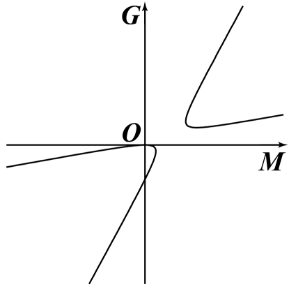
Figure 3.2: The hyperbola $C$

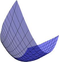
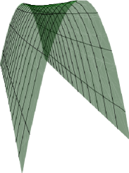
Figure 3.3: The surfaces $f$ (blue) and $\tilde{f}$ (green) viewed from $\xi(\theta_{1})$ and $\xi(\tilde{\theta}_{1})$, respectively. These contours have the same curvatures.

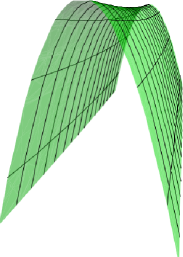
Figure 3.4: The surfaces $f$ and $\tilde{f}$ viewed from $\xi(\theta_{2})$ and $\xi(\tilde{\theta}_{2})$, respectively. These contours have the same curvatures.

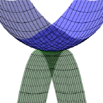
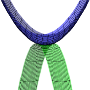
Figure 3.5: The surface $f$ rotated by angle $-\theta_{1}$ in the $XY$-plane with the surface $\tilde{f}$ rotated by angle $-\tilde{\theta}_{1}$ in the $XY$-plane, and the surface $f$ rotated by angle $-\theta_{2}$ in the $XY$-plane with the surface $\tilde{f}$ rotated by angle $-\tilde{\theta}_{2}$ in the $XY$-plane, viewed from $\xi((1,0,0))$.

3.3 Obtaining Gaussian curvature

According to Section 3.1, we can obtain all of the second order information of the surface by the contour of projections from three distinct directions. In particular, we can obtain the Gaussian curvature. In this section, we discuss obtaining just the Gaussian curvature $K$.

By (3.2), we have

$$k_{\theta_{1}}k_{\theta_{2}}=\dfrac{a_{20}^{2}a_{02}^{2}}{(a_{20}\cos^{2}\theta_{1}+a_{02}\sin^{2}\theta_{1})(a_{20}\cos^{2}\theta_{2}+a_{02}\sin^{2}\theta_{2})}.$$

Hence if

$$\dfrac{a_{20}a_{02}}{(a_{20}\cos^{2}\theta_{1}+a_{02}\sin^{2}\theta_{1})(a_{20}\cos^{2}\theta_{2}+a_{02}\sin^{2}\theta_{2})}=1,$$ (3.19)

then $K=k_{\theta_{1}}k_{\theta_{2}}$. If $\theta_{1}$, $\theta_{2}$ satisfy (3.19), then we say that $\xi_{\theta_{1}},\xi_{\theta_{2}}$ are contour-conjugate each other. Now we consider the existence of the contour-conjugate. Since (3.19) is equivalent to

$$a_{20}-a_{02}=0\quad\text{or}\quad a_{20}\dfrac{\cos^{2}\theta_{2}}{\sin^{2}\theta_{2}}=a_{02}\dfrac{\sin^{2}\theta_{1}}{\cos^{2}\theta_{1}},$$ (3.20)

we have the following proposition.

Proposition 3.6.

Let $p$ be a point that is not flat umbilic on a regular surface. If $p$ is an umbilic point, then any pair of two directions are contour-conjugates at $p$. If $K(p)>0$ and $p$ is not an umbilic point, then any direction has two contour-conjugates at $p$, and if $K(p)<0$ there are no contour-conjugate for any direction at $p$.

Example 3.7.

Let us set

$$f(u,v)=\left(u,v,\dfrac{u^{2}}{2}+v^{2}\right)$$

and

$$\theta_{1}=\pi/4,\quad\theta_{2}=\operatorname{arccot}(\sqrt{2}).$$

Then, since $\theta_{1}$ and $\theta_{2}$ satisfy (3.20), they are contour-conjugate (see Figure 3.6), namely, the product of the curvatures with respect to these directions equals $2$, the Gaussian curvature of $f$ at $0$.

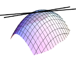
Figure 3.6: Contour-conjugate directions

4 Normal curvature and Euler’s formula

In this appendix, we give a similar formula to Theorem 3.3 for the normal curvatures. To obtain $a_{20},a_{02}$, we have another expression by using Euler’s formula (see [19, p 214], for example). In the same setting as in Section 3.1, let $\theta_{1}$, $\theta_{2}$, $\theta_{3}$ be the distinct angles $(0<\theta_{1},\theta_{2},\theta_{3}<\pi)$. Let $k_{i}^{n}$ $(i=1,2,3)$ be the normal curvatures of $f$ with respect to $\xi(\theta_{i})$, and let $M^{n}_{ij}=(k_{i}^{n}+k_{j}^{n})/2$, $G^{n}_{ij}=k_{i}^{n}k_{j}^{n}$. By Euler’s formula, we have

$$\sin^{4}(\theta_{i}-\theta_{j})M^{2}-2M_{ij}^{n}\sin^{2}(\theta_{i}-\theta_{j})M+\cos^{2}(\theta_{i}-\theta_{j})\sin^{2}(\theta_{i}-\theta_{j})G$$ (4.1)

$$\hskip 42.67912pt+\left((M_{ij}^{n})^{2}-G_{ij}^{n}\cos^{2}(\theta_{i}-\theta_{j})\right)=0.$$

For $ij=12,23,31$, these equations form a linear system

$${\begin{pmatrix}\sin^{4}(\theta_{1}-\theta_{2})&-2M_{12}^{n}\sin^{2}(\theta_{1}-\theta_{2})&\cos^{2}(\theta_{1}-\theta_{2})\sin^{2}(\theta_{1}-\theta_{2})\\ \sin^{4}(\theta_{2}-\theta_{3})&-2M_{23}^{n}\sin^{2}(\theta_{2}-\theta_{3})&\cos^{2}(\theta_{2}-\theta_{3})\sin^{2}(\theta_{2}-\theta_{3})\\ \sin^{4}(\theta_{3}-\theta_{1})&-2M_{31}^{n}\sin^{2}(\theta_{3}-\theta_{1})&\cos^{2}(\theta_{3}-\theta_{1})\sin^{2}(\theta_{3}-\theta_{1})\end{pmatrix}}{\begin{pmatrix}M^{2}\\ M\\ G\end{pmatrix}}$$

$$\hskip 28.45274pt={\begin{pmatrix}(M_{12}^{n})^{2}-G_{12}^{n}\cos^{2}(\theta_{1}-\theta_{2})\\ (M_{23}^{n})^{2}-G_{23}^{n}\cos^{2}(\theta_{2}-\theta_{3})\\ (M_{31}^{n})^{2}-G_{31}^{n}\cos^{2}(\theta_{3}-\theta_{1})\end{pmatrix}}.$$

By Cramer’s rule, we have the expressions

$$M=\dfrac{\det P^{n}}{\det V^{n}},\quad G=\dfrac{2\det L^{n}}{\det V^{n}}$$

under the condition $\det V^{n}\neq 0$, where $V^{n}=\big{(}x_{5},x_{3},x_{4}\big{)}$, $L^{n}=\big{(}x_{6},x_{5},x_{4}\big{)}$, $P^{n}=\big{(}x_{6},x_{3},x_{4}\big{)}$, $x_{3},x_{4}$ are in (3.10), (3.11) respectively, and

$$x_{5} ={\vphantom{\big{(}M_{12}^{n},M_{23}^{n},M_{31}^{n}\big{)}}}^{t}{\!\big{(}M_{12}^{n},M_{23}^{n},M_{31}^{n}\big{)}}$$

$$x_{6} ={\vphantom{\left(\dfrac{(M_{12}^{n})^{2}-G_{12}^{n}\cos^{2}(\theta_{1}-\theta_{2})}{\sin^{2}(\theta_{1}-\theta_{2})},\dfrac{(M_{23}^{n})^{2}-G_{23}^{n}\cos^{2}(\theta_{2}-\theta_{3})}{\sin^{2}(\theta_{2}-\theta_{3})},\right.}}^{t}{\!\left(\dfrac{(M_{12}^{n})^{2}-G_{12}^{n}\cos^{2}(\theta_{1}-\theta_{2})}{\sin^{2}(\theta_{1}-\theta_{2})},\dfrac{(M_{23}^{n})^{2}-G_{23}^{n}\cos^{2}(\theta_{2}-\theta_{3})}{\sin^{2}(\theta_{2}-\theta_{3})},\right.}$$

$$\hskip 170.71652pt\left.\dfrac{(M_{31}^{n})^{2}-G_{31}^{n}\cos^{2}(\theta_{3}-\theta_{1})}{\sin^{2}(\theta_{3}-\theta_{1})}\right).$$

Competing Interests

The authors declare that they have no competing interests.

Author’s Contributions

The current paper was jointly developed by the three authors in the seminar discussions. All the authors equally contributed.

References

- [1] R. Cipolla and P. Giblin, Visual motion of curves and surfaces, Cambridge Univ. Press, Cambridge, 2000.
- [2] R. Cipolla and A. Blake, A surface shape from the deformation of apparent contours, Int. J. Comput. Vision 9 (1992), 83–112.
- [3] R. Cipolla, Active visual inference of surface shape, Lecture Notes in Computer Science 1016 Springer-Verlag Berlin Heidelberg, 1996.
- [4] J. Damon, P. Giblin and G. Haslinger, Local image features resulting from -dimensional image features, illumination and movement, I, Internat. J. Computer Vision 82 (2009), 25-47.
- [5] J. Damon, P. Giblin and G. Haslinger, Local image features resulting from -dimensional image features, illumination and movement, II SIAM Journal of Imaging Sciences 4 (2011), 386-412.
- [6] J. Damon, P. Giblin and G. Haslinger, Local features in natural images via singularity theory, Lecture Notes in Math. 2165, Springer, 2016.
- [7] R. Fabbri and B. Kimia, Multiview differential geometry of curves, Int. J. Comput. Vis. 120 (2016), no. 3, 324–346.
- [8] J. F. Norman, J. T. Todd and F. Phillips, The perception of surface orientation from multiple sources of optical information, Perception Psychophysics 57 (1995), 629–636.
- [9] T. Fukui, M. Hasegawa and K. Nakagawa, Contact of a regular surface in Euclidean 3-space with cylinders and cubic binary differential equations, J. Math. Soc. Japan, 69 (2017), 819–847.
- [10] P. Giblin and R. Weiss, Reconstruction of surfaces from profiles, Proc. 1st International Conference on Computer Vision, (1987) 136–144.
-
[11]
H. W. Gould,
Table for Fundamentals of Series: Part I: Basic
Properties of Series and Products,
unpublished manuscript notebooks.
https://www.math.wvu.edu/~gould/ - [12] S. Izumiya, M. C. Romero-Fuster, M. A. S. Ruas and F. Tari, Differential Geometry from a Singularity Theory Viewpoint. World Scientific Pub. Co Inc. 2015.
- [13] J. J. Koenderink, What does the occluding contour tell us about solid shape?, Perception, 13 (1984), 321–330.
- [14] J. J. Koenderink, Solid shape, MIT Press Series in Artificial Intelligence. MIT Press, Cambridge, MA, 1990.
- [15] J. J. Koenderink and A. J. Van Doorn, The shape of smooth objects and the way contours end, Perception 11, 129-137.
- [16] I. A. Koganand P. J. Olver, Invariants of objects and their images under surjective maps, Lobachevskii J. Math. 36 (2015), no. 3, (2015), 260–285.
- [17] G. Li and S. W. Zucker, A differential geometrical model for contour-based stereo correspondence, Proc. IEEE Workshop on Variational, Geometric, and Level Set Methods in Computer Vision, Nice, France, 2003.
- [18] M. McKiernan, On the th Derivative of Composite Functions, Amer. Math. Monthly 63 (1956), no. 5, 331–333.
- [19] B. O’Neill, Elementary differential geometry, Revised second edition. Academic Press, Amsterdam, 2006.
- [20] K. Saji, M. Umehara, and K. Yamada, The duality between singular points and inflection points on wave fronts, Osaka J. Math. 47 (2010), no. 2, 591–607.
- [21] S. Shiba and M. Umehara, The behavior of curvature functions at cusps and inflection points, Differential Geom. Appl. 30 (2012), no. 3, 285–299.
- [22] J. Y. Zheng, Acquiring -D models from sequences of contours, IEEE Transactions on Pattern Analysis and Machine Intelligence, 16 (1994), no. 2, 163–178.