Stockholm University, AlbaNova University Centre, SE-106 91 Stockholm
Bimetric polytropes
Abstract
We present a method for solving the constraint equations in the Hassan–Rosen bimetric theory to determine the initial data for the gravitational collapse of spherically symmetric dust. The setup leads to equations similar to those for a polytropic fluid in general relativity, here called a generalized Lane–Emden equation. Using a numerical code which solves the evolution equations in the standard 3+1 form, we also obtain a short term development of the initial data for these bimetric polytropes. The evolution highlights some important features of the bimetric theory such as the interwoven and oscillating null cones representing the essential nonbidiagonality in the dynamics of the two metrics. The simulations are in the strong-field regime and show that, at least at an early stage, the collapse of a dust cloud is similar to that in general relativity, and with no instabilities, albeit with small oscillations in the metric fields.
Keywords:
Modified gravity, Ghost-free bimetric theory, Numerical bimetric relativity1 Introduction
In comparison to general relativity (GR), the phenomenology of the Hassan-Rosen (HR) bimetric theory Hassan:2011zd ; Hassan:2011ea ; Hassan:2017ugh ; Hassan:2018mbl is at an early stage, and the full extent of its physical features is still unknown. In GR, numerical relativity plays an important role in theoretical astrophysics to clarify structure formation and growth, or formation processes of black holes. Only by means of numerical simulation and experiments, it is possible to get a theoretical understanding of such phenomena occurring in nature Shibata:2015nr ; Baumgarte:2010nr ; Gourgoulhon:2012trip ; Alcubierre:2012intro ; Bona:2009el . In particular, numerical relativity is essential in analyzing strong-field gravitational systems to interpret gravitational wave detections Abbott:2016blz . Similar remarks also hold for the HR theory. In order to perform bimetric numerical simulations (and discriminate bimetric from GR predictions), many questions need to be addressed; for example Shibata:1999va :
-
(1)
Which initial data solve the bimetric constraints for gravitational collapse?
-
(2)
Which formalism to use for stable bimetric numerical evolution?
-
(3)
What are appropriate gauge conditions?
-
(4)
What algorithms provide numerical stability?
-
(5)
What are suitable boundary conditions for numerical grids?
-
(6)
What is a good method for finding the apparent horizon?
To obtain reliable numerical results, all of these issues have to be resolved.
This work belongs to a series of papers in which we aim to investigate the above issues. Earlier papers in this series establish the bimetric equations in the standard 3+1 form Kocic:2018ddp , and calculate the ratio of lapse functions for the case of spherical symmetry Kocic:2019zdy . In the current paper, we present a method for solving the bimetric constraints to determine the initial data for the gravitational collapse of dust in the HR theory. Using a numerical code based on the equations of motion in the standard 3+1 form, we then obtain a short term development of the initial data. Obtaining a long term bimetric development is the subject of ongoing work. In order to achieve a more stable numerical evolution, Torsello:2019tgc establishes the covariant Baumgarte–Shapiro–Shibata–Nakamura (cBSSN) formalism Shibata:1995we ; Baumgarte:1998te ; Brown:2005a ; Brown:2009a ; Brown:2012a for bimetric relativity. A class of gauge conditions specific to the HR theory are treated in Torsello:meang .
This paper is structured as follows. The rest of this section summarizes the results by examples; it also reviews the basic equations. Section 2 poses and solves the bimetric constraint equations. Section 3 highlights the properties of the evolution of the initial data. The paper ends with a brief discussion and outlook.
1.1 Summary of results
We consider the case where the two metric sectors share the same spherical symmetry Torsello:2017ouh . In GR, the kinematical and dynamical parts of a metric field can be separated using the 3+1 formalism Arnowitt:1962hi ; York:1979aa . The same procedure can be applied to bimetric theory using a suitable parametrization based on the geometric mean metric Kocic:2018ddp . In this context, the general form of the two metrics in spherical polar coordinates reads,
| (1a) | ||||
| (1b) | ||||
where and denote the lapse functions, and are the radial components of the shift vectors, and denote the nontrivial components of the spatial vielbeins. In addition, we also evolve the nonzero components of the extrinsic curvature,
| (2) |
The radial components of the shift vectors are conveniently redefined in terms of the mean shift and the separation parameter Kocic:2018ddp ,
| (3) |
In this parametrization, the lapses , , and the mean shift do not appear in the constraint equations. All the variables in (1)–(3) are functions of . We let matter (if any) be coupled to only one of the metric sectors, here .
We start from the development of existing GR initial data for , hereinafter called the reference GR solution. At this stage we decouple ; the bimetric theory is reduced to two copies of GR where we only consider the evolution in the -sector containing the collapsing matter (letting evolve in parallel, for instance, a Minkowski solution). The bimetric interaction will be engaged in a second stage, treating the bimetric collapse after knowing the behavior of the reference GR solution.
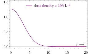
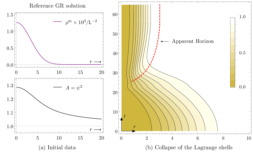
As a reference GR solution, we consider a spherical dust cloud with arbitrary density profile at . The initial data can be constructed using the time symmetric initial condition where the extrinsic curvature is vanishing, assuming the conformally flat spatial metric. The initial values for the density with a Gaussian profile and the corresponding metric field are shown in figure 1. The development of this initial data forms a black hole Nakamura:1980 .
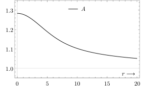
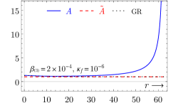
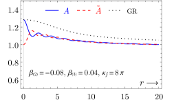
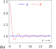
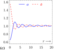
After constructing the reference GR solution, we engage the two sectors through the bimetric interaction and solve the constraint equations for the metric fields, keeping the same matter profile coupled to . This results in a system of coupled differential equations whose solution depends on the parameters of the HR theory. The construction of the bimetric initial data is the topic of section 2. Typical initial values for the metric fields and which are far from the GR limit are shown in figure 2. These fields carry physical content for the observers in the respective metric sector; they roughly correspond to gravitational potentials in the Newtonian limit.
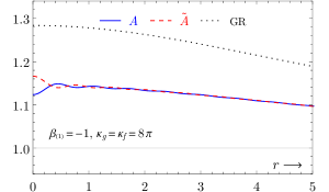
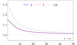
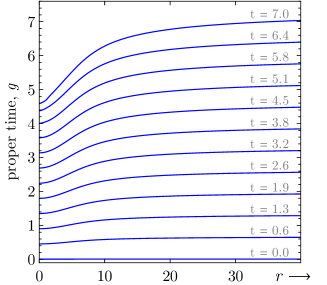
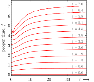
Finally, as described in section 3, we numerically evolve the initial data. The simulations are not long enough to shed light on the end point of gravitational collapse. Nevertheless, the bimetric collapse of the dust cloud stays very close to the reference GR solution, as illustrated in figure 3. More details about the gravitational collapse in the GR limit are given in subsection 3.3 (see also figures 5 and 17).
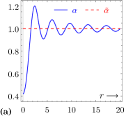
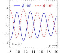
To highlight the bimetric features in the physical content, we employ causal diagrams that display metric configurations according to the method given in Kocic:cdg . From these diagrams one can read-off the oscillation frequencies of the metric fields in space and time. The causal diagrams are based on the fact that the possible configurations of two metrics can be visualized in terms of the null cone intersections Hassan:2017ugh , as shown in figure 4(a). Coordinate transformations only deform the null cones, keeping the nature of their intersections. This gives an invariant picture of the bimetric spacetime. The causal diagram for the evolution of the initial data from figure 2 is plotted in figure 4(b), showing the leading frequencies in the dynamics of the metrics fields.
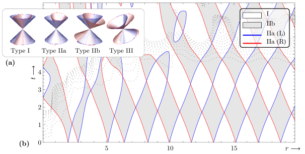
Figure 4 also displays how the metric configurations are interwoven in space and time. Note that the metrics have been constructed to be simultaneously diagonalizable at the initial hypersufrace. Such “bidiagonal slices” may locally reoccur during the evolution (horizontally slicing the white rhomboid-like patches in some regions in figure 4). Notwithstanding, the two metrics are in general not simultaneously diagonalizable, and the solution lacks a timelike Killing vector field (so it cannot be made stationary by any coordinate transformation). Finally, the dotted lines in figure 4 indicate the regions where the constraints get more violated. These are the artifacts of the numerical simulation and indicate a departure from the bimetric solution. More elaborate comments on the evolution and numerical simulations are found in section 3.
1.2 Basic equations
We consider the metrics and coupled through the ghost-free bimetric potential deRham:2010ik ; deRham:2010kj ; Hassan:2011vm ,
| (4) |
Here, denotes the principal square root of the (1,1) tensor field , and are the elementary symmetric polynomials (the principal scalar invariants of ). The potential is parametrized by dimensionless real constants with an overall length scale in the geometrized units . The particular form of the potential is dictated by the necessary condition for the absence of ghosts Creminelli:2005qk , where the dynamics of each metric is given by a separate Einstein-Hilbert term in the action Hassan:2011zd . The principal branch of the square root ensures an unambiguous definition of the theory Hassan:2017ugh .
The resulting bimetric field equations are (here stated in the operator form),
| (5a) | ||||||
| (5b) | ||||||
where and are the Einstein tensors of the two metrics, and are Einstein’s gravitational constants, and are the stress–energy tensors of the matter fields each minimally coupled to a different metric sector, and and are the contributions of the bimetric potential (4), also called the bimetric stress–energy tensors. The functions in (5) encapsulates the variation of the bimetric potential with respect to the metrics,
| (6) |
The bimetric stress–energy tensors satisfy the following identities Hassan:2014vja ; Damour:2002ws ,
| (7a) | ||||
| (7b) | ||||
where and are the covariant derivatives compatible with and , respectively. Assuming that the matter conservation laws hold, and , the field equations (5) imply the bimetric conservation law,
| (8) |
The two equations in (8) are not independent according to the differential identity (7b).
The 3+1 decomposition.
The structure of the bimetric field equations is equivalent to having two copies of GR with the additional stress–energy contributions and coupled through (7a); hence, their 3+1 split is straightforward, provided that one knows the projections of and Kocic:2018ddp . The 3+1 decomposition of (5) results in two sets of the evolution and constraint equations formally analog to those in GR Shibata:2015nr ; Baumgarte:2010nr ; Gourgoulhon:2012trip ; Alcubierre:2012intro ; Bona:2009el .
The constraint equations do not depend on the lapse functions and one shift vector because of the particular form of the potential (4). The projection of the bimetric conservation law (8) gives one additional constraint Kocic:2018ddp , equivalent to the additional constraint obtained from the Hamiltonian analysis Hassan:2018mbl (the so-called secondary constraint). Moreover, as shown in Alexandrov:2012yv ; Hassan:2018mbl , the preservation of this additional constraint relates the two lapses through a ratio, calculated for the case of spherical symmetry in Kocic:2019zdy .
Since our focus is not on the evolution equations, their standard 3+1 form is given in appendix A. The constraint equations are treated in the following section in more detail.
2 Initial data
The initial values for evolution are subject to certain constraints. In spherical symmetry, the dynamical variables are and . Also, the separation parameter defines the relative shift between the two metrics (characterizing the relative ‘off-diagonality’ of the metrics). The two lapse functions , , and the mean shift are kinematical variables and do not appear in the constraint equations. Hence, we need to specify the following metric functions of at : , , , , , , , , and . These functions are constrained by five equations, which leaves a lot of freedom in choosing their initial values. In the rest of this section, we state the constraint equations, solve for a reference GR solution, and construct the related bimetric initial data.
2.1 Constraint equations
To write down the constraint equations, we need the 3+1 decomposition of the stress–energy tensors. Let and denote the normal, tangential and spatial projections of the total stress–energy tensors in the respective sector. These projections sum up the contribution coming from the bimetric potential, denoted by the upper label “b”, and the matter contribution, denoted by the upper label “m”; for example, .
Bimetric sources.
Similarly for we have,
| (10a) | ||||
| (10b) | ||||
| (10c) | ||||
where , , and . To simplify equations, we have defined and,
| (11) |
The function encapsulates the -parameters that do not appear elsewhere. The tangential components satisfy the following identity coming from (7a),
| (12) |
Matter sources.
We assume that matter is present only in the -sector and let . In particular, we consider a perfect fluid with the stress–energy tensor Baumgarte:2010nr ; Rezzolla:2013rel ,
| (13) |
where is the rest-mass density, is the specific enthalpy, is the specific energy, is the pressure, and is the four–velocity of the fluid. The general relativistic hydrodynamic equations consist of the conservation law for , the conservation law of the baryon number, and the equation of state for the fluid, respectively given by,
| (14) |
Following the 3+1 “Valencia” formulation Banyuls:1997zz ; Rezzolla:2013rel , we rewrite (14) in the first order flux–conservative form. In spherical coordinates, the resulting equations are expressed in terms of the following conserved variables (here densitizied),
| (15) |
where is defined in (12), is the radial component of the Eulerian three-velocity of the fluid, and is the corresponding Lorentz factor,
| (16) |
The flux–conservative evolution equations for are relegated to the ancillary file.
For a pressureless fluid (dust), we have , , , and the conversion from the conserved to the primitive variables reads,
| (17) |
Finally, the calculation in Rezzolla:2013rel yields the components of the matter stress–energy tensor,
| (18a) | ||||
| (18b) | ||||
| (18c) | ||||
Bimetric constraints.
The scalar and vector constraint equations are obtained as the normal and tangential projections of the bimetric field equations (5) on the initial hypersurface. The scalar (or Hamiltonian) constraint equations are,
| (19a) | ||||||
| (19b) | ||||||
| The vector (or momentum) constraint equations are, | ||||||
| (19c) | ||||||
| (19d) | ||||||
The last two equations can be combined using the identity (12),
| (20) | ||||
The separation parameter can be determined either from (19c) or (19d).
The bimetric scalar and vector constraints (19) are the same as in GR with the addition of the bimetric sources; what is specific to the HR theory is the additional constraint obtained from the projection of the bimetric conservation law,
| (21) |
As an example of the bimetric initial data with no matter sources, consider the initial values , , , and where . These satisfy (19)–(21) and yield the bi-Minkowski solution.
2.2 Reference GR solution
As mentioned in the introduction, we start from a reference GR solution with decoupled bimetric sectors; we set and let the two sectors independently evolve in parallel. This implies , hence (21) identically vanishes at all times. The -sector is set up to develop the Minkowski solution from the initial data , , and .
The initial data for are constructed using the time symmetric initial condition,
| (22) |
also assuming a conformally flat spatial metric at with the conformal factor ,
| (23) |
At this point all the bimetric constraints except (19a) are satisfied. Hence, and must satisfy,
| (24) |
where and denotes the spherical Laplacian. Consider the initial density,
| (25) |
Here, is a free parameter and is the integral of the Gaussian distribution. This density is the same as in Nakamura:1980 for . The solution to (24) becomes,
| (26) |
An example of the initial data for is shown in figure 5; the evolution of these data is treated in section 3, with the results shown in the right panel of figure 5.
2.3 Bimetric polytrope
We now engage the bimetric interaction, keeping the same initial density of dust as in the reference GR solution. We again use the time symmetric initial condition with the conformally flat spatial metrics in each sectors,
| (27a) | ||||||||
| (27b) | ||||||||
We set but allow for arbitrary -parameters. The metric configuration is therefore of Type I at the initial hypersurface with simultaneously diagonal and .
At the moment of time symmetry where , , and , the constraint equations (19c), (19d), and (21) are automatically satisfied. Thus, we only have to consider the scalar constraints (19a) and (19b); these form a system of generalized Lane–Emden equations,
| (28a) | ||||||
| (28b) | ||||||
In astrophysics Chandra:1957intro , the Lane–Emden equation represents a self–gravitating spherically symmetric fluid with the polytropic equation of state ; in that context, satisfies the Lane–Emden equation . Now, interpreting the conformal factors as gravitational potentials in the Newtonian limit, the metric fields obey deformed polytropic equations of states (where the polytropic index becomes definite for a specific -model in vacuum, ). In other words, engaging the second metric in an existing GR solution introduces a fluid with nontrivial features in both sectors; this gives the name “bimetric polytrope” (referred to as “pure” when ). The departure from GR is controlled by the overall factors and .
Given , the system (28) should be solved for and . We choose asymptotic boundary conditions where , , and at infinity. This imposes a necessary condition for the -parameters; for example, requiring implies,
| (29) |
which fixes and in terms of the other parameters. Moreover, in spherical symmetry, the metric components must be even functions of Alcubierre:2010is . Therefore, we use the Neumann boundary conditions at requiring and . Note that we may still choose some arbitrary positive values for and at .
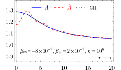
To summarize: beside , , , , , , and the density , we are free to choose and at , and their ratio at . Note that the departure from the reference GR solution is a smooth function of the free parameters (as found by inspection). The GR limit of the HR theory is given by Schmidt-May:2015vnx ; Akrami:2015qga ; Berezhiani:2007zf ; Martin-Moruno:2013wea . Examples of initial data for different parameter values are shown in figure 6.
| (1) | 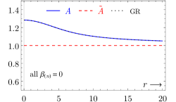 |
(2) | 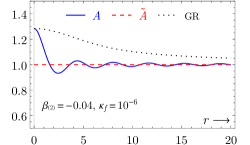 |
| (3) | 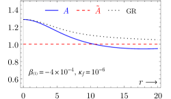 |
(4) | 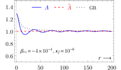 |
| (5) | 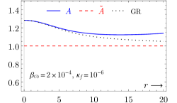 |
(6) |  |
| (7) | 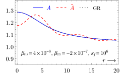 |
(8) |  |
| (9) | 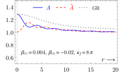 |
(10) |  |
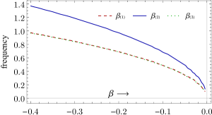
From the plots we observe higher oscillation frequencies for large -parameters, which is compliant with the properties of the Lane–Emden equation Chandra:1957intro ; Christensen:1994ic . The leading frequencies for the pure bimetric polytropes are shown in figure 7.
The preservation of the additional constraint (21) relates the two lapses through where and are functions of dynamical variables Alexandrov:2012yv ; Hassan:2018mbl . For the case of spherical symmetry, these functions are established in Kocic:2019zdy . The relation holds at all times, including where it depends on the initial data as shown in figure 8 and 9.
Symmetries in the shapes of and at may be used as a guideline to what kind of gauge conditions are preferable for the time slicing, e.g., singling out (c) from figure 9.
3 Development of the initial data
Here we present the solutions obtained from the bimetric initial data. We use a free evolution scheme where the constraint equations are solved at the initial surface and the initial data developed by the bimetric evolution equations. The constraint equations are used as error estimators during the evolution. To evolve the equations, we have written a numerical relativity code package for the bimetric theory, bim-solver. The package is written in C++ and provides a framework that combines the evolution equations generated in Mathematica into a functioning bimetric numerical relativity code. The code is OpenMP parallelized OpenMP and supports MPI MPISpec . The implementation details for bim-solver will be given elsewhere.
3.1 Formalism and numerical methods
The evolution equations are of the standard 3+1 form, given in appendix A. Because of the coordinate singularity at , the equations of motion have to be regularized; for this, we use the regularization procedure described in Alcubierre:2004gn ; Ruiz:2007rs ; Alcubierre:2010is ; Alcubierre:2012intro . The regularized equations are relegated to an ancillary file (which can be found on arXiv).
The equations are solved using the finite difference approximation in a uniform grid. The implemented spatial difference scheme is centered in space and with arbitrary finite difference order (we have used up to the sixth order). For the time evolution, we employ the method of lines (MoL) using Runge–Kutta (RK) and iterated Crank-Nicholson (ICN) integration. Moreover, Kreiss-Oliger (KO) dissipation has been added for stability Kreiss:1973aa ; Gustafsson:2013KO . As diagnostics, the -norm of the constraint equations is monitored.
Boundary conditions should be handled appropriately to avoid spurious back reflections of waves causing numerical instabilities. As mentioned, the inner boundaries are fixed by mirroring the grid cells around . The outer boundaries are handled by imposing open boundary conditions. We assume that no waves are traveling in from outside of the domain of influence. Hence, the ghost cells at are updated by extrapolating the interior solution, assuming continuity at the boundary. The extrapolation of the fields is to first order; hence, small unphysical errors are generated in numerical simulations. To delay their propagation, we set the right grid boundary at large radii.
The gauge variables are , , and where the lapses related through . The simplest gauge choices are the algebraic: , , or . The last choice fixes to one the lapse function of the geometric mean metric Kocic:2018ddp (other gauges specific to the HR theory are discussed in Torsello:meang ). Besides using the algebraic gauge conditions, the numerical code also implements the maximal slicing, in this paper used with respect to .
To detect black hole formation, the code implements an apparent horizon finder in both sectors. In spherical symmetry, a marginally outer trapped surface (MOTS) is given by Baumgarte:1996aa ; Thornburg:2006zb ; Shibata:2015nr ,
| (30) |
The apparent horizon is the outermost MOTS at which (30) is satisfied. The solution is obtained using a root-finding algorithm. Alternatively, the function can be plotted, and the apparent horizons determined graphically.
3.2 Simulations
Here we give the numerical details for the simulations and show representative results. We have performed two kinds of simulations:
-
(i)
benchmark (diagnostics) simulation for the reference GR initial data,
-
(ii)
simulations with the engaged bimetric interactions.
For the GR simulation, the grid spacing is with the outer boundary at . The spatial difference scheme is of the fourth order. The integration employs the method of lines with the third order Runge–Kutta and the Courant–Lax factor (CFL) of . The added Kreiss–Oliger dissipation is of the fourth order with the coefficient . The lapse is evolved using maximal slicing. The evolution is stable and goes beyond . The results of the GR simulation are shown in figure 5, which are compatible with Nakamura:1980 .
After the control benchmark, we consider the development of the bimetric initial data constructed in subsection 2.3. Here we use the grid spacing with the outer boundary pushed to and the CFL decreased to . The initial conditions with the evolution of the metric components are shown in figure 10(a).
| (a) | 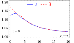 |
(b) | 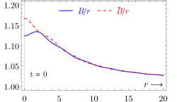 |
| (c) | 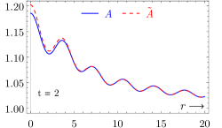 |
(d) | 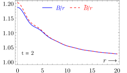 |
| (e) | 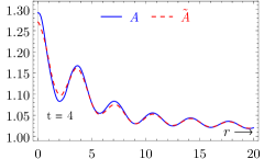 |
(f) | 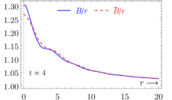 |
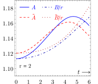
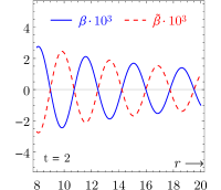
The metric components have a tendency to become bi-proportional, and , at least over a short time period as in figure 12. Note that the null cones oscillate over the time; the same figure shows the radial components of the shift vectors at and .
(a) 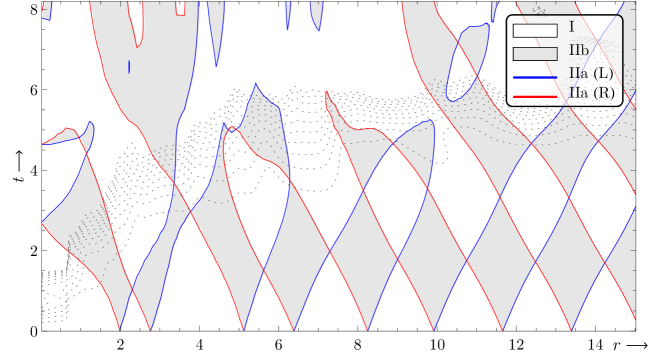
(b) 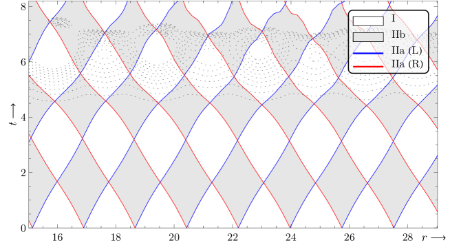
The lapses are evolved using the maximal slicing with respect to ; the proper times of the Eulerian observers for and are shown in figure 11. Time is slowed down near the coordinate origin because of the failed regularization. In contrast to the GR simulations that run beyond , the bimetric evolutions fail within , mostly because of the violated boundary conditions. The main cause of the instability are irregularities coming from round-off errors when calculating the lapse ratio and the corresponding spatial derivatives near . The causal diagram for the solution near the coordinate origin is shown in figure 13(a). The dotted lines indicate surface levels of the -norm of the scalar constraint violations with separation . The irregularities are visible close to the origin. As noted before, the white regions are Type I (bidiagonal) and the shaded Type IIb. The edges are Type IIa, either with the common left- or right-null directions. The intersections of two left-right Type IIa edges are of Type I. The causal diagram at larger radii is given in figure 13(b), with the constraint violations in figure 14. The solution is trustworthy for , which is enough to conclude the time-dependent nonbidiagonality in the dynamics of the two metrics represented by the interwoven and oscillating null cones.
Finally, we have performed several thousands of simulations for different parameter values, and the earlier shown examples are typical. An important observation is that the pure bimetric polytropes (vacuum solutions) share the same property: they are generically nonbidiagonal and nonstationary; an example is shown in figure 15, where the causal diagram is trustworthy for . The pure bimetric polytropes contradict the bimetric analogue of Birkhoff’s theorem Birkhoff:1923 ; Jebsen:1921 ; Jebsen:2005 , which is compatible with the findings in Kocic:2017hve .
3.3 Gravitational collapse
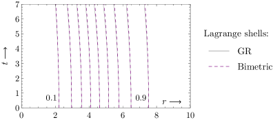
The simulations are not long enough to shed light on the end point of gravitational collapse. Nevertheless, the present numerical experiments show that the collapse of the dust cloud follows the pattern from the reference GR solution, showing no instabilities. A physically realistic solution is illustrated in figure 17, where the initial data are close to GR and . The time variation of the Lagrange shells is shown in panel (b); the plot is almost the same as in figure 5 (the plots can be compared since the evolution of the time gauge are similar for the two solutions for ).
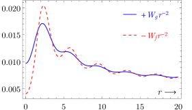
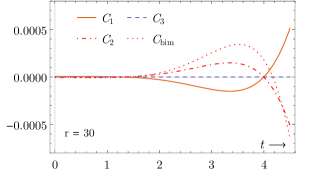
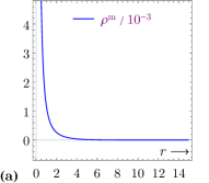
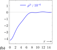
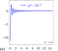
The stress–energy contributions coming from the matter, , and the bimetric potential, , are shown in figures 16(a) and (b). These contributions enter the constraint equations (19a) and (28a). In the GR limit, is more than times smaller than , due to small -parameters. For comparison, figure 16(c) shows a large contribution from the bimetric potential when the initial data are far from GR (as in figure 2).
4 Discussion and outlook
In this work, we have:
-
(i)
presented a method for solving the constraint equations in the Hassan–Rosen theory to determine bimetric initial data by deforming the existing GR initial data,
-
(ii)
obtained the generalized Lane–Emden equations for the bimetric initial data specifically assuming the conformally flat spatial metrics at the moment of time symmetry,
-
(iii)
solved for and analyzed the obtained initial data,
-
(iv)
evolved the initial data using a new numerical code for bimetric relativity.
The results once again point out the importance of nonbidiagonality in the dynamics of the two metrics. The authors in Babichev:2014oua showed that to have dynamically stable solutions, nondiagonal metric elements are needed. Moreover, Torsello:2017cmz concludes that considering static black hole solutions in the HR theory is insufficient and that a full dynamical treatment needs to be performed in order to investigate the end point of gravitational collapse. Finally, even in the absence of external matter sources, the bimetric solutions are essentially nonbidiagonal and nonstationary; hence, our results disprove the analogue version of Birkhoff’s theorem for bimetric theory, which is compatible with the findings in Kocic:2017hve .
The initial data for bimetric polytropes requires negative -parameters because of the boundary conditions that are imposed on the constraint equations (28) (see figure 7). This would correspond to an imaginary Fierz–Pauli mass obtained from the spectrum of linearized mass eigenstates on the proportional backgrounds Hassan:2012wr ; Schmidt-May:2015vnx ; Luben:2018ekw . However, the bimetric polytropes are nonproportional solutions in a strong-field regime with the initial conditions that assume conformal flatness. In addition, we are more restrictive on the choice of and in (29) than needed to define the Fierz–Pauli mass, which could affect the conclusions on its sign. This suggests that the properties of the bimetric parameter space should be further investigated.
A future goal is to obtain a long term development of the initial data. For this purpose, the covariant BSSN formalism is established in Torsello:2019tgc , and various gauge conditions specific to bimetric relativity are investigated in Torsello:meang . Work in progress deals with the implementation of BSSN in bim-solver to obtain stable numerical simulations in spherical symmetry.
Acknowledgments
We would like to thank Giovanni Camelio for a careful reading of the manuscript.
Appendix A Evolution equations
The evolution equations for the spatial metrics are,
| (31a) | ||||||
| (31b) | ||||||
The evolution equations for the extrinsic curvatures are,
| (32a) | ||||
| (32b) | ||||
| (32c) | ||||
| (32d) | ||||
The above set of equations is in each sector equivalent to the GR case Shibata:2015nr .
These equations are subject to the regularization procedure described in Alcubierre:2004gn ; Ruiz:2007rs ; Alcubierre:2010is ; Alcubierre:2012intro . There are two types of regularity conditions that must be satisfied. First, the parity which comes from symmetry considerations. Spherical symmetry implies that a reflection in the radial coordinate leaves metrics unchanged. After reflecting , we see that the lapses, the spatial metric components, and the corresponding components of the extrinsic curvature must be even functions of , while the shift vector must be odd. Beside the parity, the extra regularity conditions require that the manifold must be locally flat at the origin. The regularization is done in several steps (done in both sectors):
-
(i)
redefine (and similarly ),
-
(ii)
introduce:
, , ,
, and ,
-
(iii)
find the evolution equation for these variables,
-
(iv)
evolve these variables imposing the odd parity conditions.
The regularized equations are too long to write down here; they are relegated to an ancillary file, which can be found on arXiv.
References
- (1) S. F. Hassan and R. A. Rosen, Bimetric Gravity from Ghost-free Massive Gravity, JHEP 02 (2012) 126, [1109.3515].
- (2) S. F. Hassan and R. A. Rosen, Confirmation of the Secondary Constraint and Absence of Ghost in Massive Gravity and Bimetric Gravity, JHEP 04 (2012) 123, [1111.2070].
- (3) S. F. Hassan and M. Kocic, On the local structure of spacetime in ghost-free bimetric theory and massive gravity, JHEP 05 (2018) 099, [1706.07806].
- (4) S. F. Hassan and A. Lundkvist, Analysis of constraints and their algebra in bimetric theory, JHEP 08 (2018) 182, [1802.07267].
- (5) M. Shibata, Numerical Relativity. World Scientific Publishing, 2015.
- (6) T. Baumgarte and S. Shapiro, Numerical Relativity. Cambridge University Press, 2010.
- (7) É. Gourgoulhon, 3+1 Formalism in General Relativity: Bases of Numerical Relativity. Lecture Notes in Physics. Springer Berlin Heidelberg, 2012.
- (8) M. Alcubierre, Introduction to 3+1 Numerical Relativity. OUP Oxford, 2012.
- (9) C. Bona, C. Palenzuela-Luque and C. Bona-Casas, Elements of Numerical Relativity and Relativistic Hydrodynamics: From Einstein’s Equations to Astrophysical Simulations. Springer Berlin Heidelberg, 2009.
- (10) LIGO Scientific, Virgo collaboration, B. P. Abbott et al., Observation of Gravitational Waves from a Binary Black Hole Merger, Phys. Rev. Lett. 116 (2016) 061102, [1602.03837].
- (11) M. Shibata, 3-D numerical simulation of black hole formation using collisionless particles: Triplane symmetric case, Prog. Theor. Phys. 101 (1999) 251–282.
- (12) M. Kocic, Geometric mean of bimetric spacetimes, 1803.09752.
- (13) M. Kocic, A. Lundkvist and F. Torsello, On the ratio of lapses in bimetric relativity, 1903.09646.
- (14) F. Torsello, M. Kocic, M. Högås and E. Mortsell, Covariant BSSN formulation in bimetric relativity, 1904.07869.
- (15) M. Shibata and T. Nakamura, Evolution of three-dimensional gravitational waves: Harmonic slicing case, Phys. Rev. D52 (1995) 5428–5444.
- (16) T. W. Baumgarte and S. L. Shapiro, On the numerical integration of Einstein’s field equations, Phys. Rev. D59 (1999) 024007, [gr-qc/9810065].
- (17) J. D. Brown, Conformal invariance and the conformal-traceless decomposition of the gravitational field, Phys. Rev. D 71 (May, 2005) 104011.
- (18) J. D. Brown, Covariant formulations of Baumgarte, Shapiro, Shibata, and Nakamura and the standard gauge, Phys. Rev. D 79 (May, 2009) 104029.
- (19) J. D. Brown, P. Diener, S. E. Field, J. S. Hesthaven, F. Herrmann, A. H. Mroué et al., Numerical simulations with a first-order BSSN formulation of Einstein’s field equations, Phys. Rev. D 85 (Apr, 2012) 084004.
- (20) F. Torsello, The mean gauges in bimetric relativity, (in preparation) .
- (21) F. Torsello, M. Kocic, M. Högås and E. Mortsell, Spacetime symmetries and topology in bimetric relativity, Phys. Rev. D97 (2018) 084022, [1710.06434].
- (22) R. L. Arnowitt, S. Deser and C. W. Misner, The dynamics of general relativity, Gen. Rel. Grav. 40 (2008) 1997–2027, [gr-qc/0405109].
- (23) J. W. York, Jr., Kinematics and Dynamics of General Relativity, pp. 83–126.
- (24) T. Nakamura, K.-i. Maeda, S. Miyama and M. Sasaki, General Relativistic Collapse of an Axially Symmetric Star. I: The Formulation and the Initial Value Equations, Progress of Theoretical Physics 63 (04, 1980) 1229–1244.
- (25) M. Kocic, Note on bimetric causal diagrams, (to appear) .
- (26) C. de Rham and G. Gabadadze, Generalization of the Fierz-Pauli Action, Phys. Rev. D82 (2010) 044020, [1007.0443].
- (27) C. de Rham, G. Gabadadze and A. J. Tolley, Resummation of Massive Gravity, Phys. Rev. Lett. 106 (2011) 231101, [1011.1232].
- (28) S. F. Hassan and R. A. Rosen, On Non-Linear Actions for Massive Gravity, JHEP 07 (2011) 009, [1103.6055].
- (29) P. Creminelli, A. Nicolis, M. Papucci and E. Trincherini, Ghosts in massive gravity, JHEP 09 (2005) 003, [hep-th/0505147].
- (30) S. F. Hassan, A. Schmidt-May and M. von Strauss, Particular Solutions in Bimetric Theory and Their Implications, Int. J. Mod. Phys. D23 (2014) 1443002, [1407.2772].
- (31) T. Damour and I. I. Kogan, Effective Lagrangians and universality classes of nonlinear bigravity, Phys. Rev. D66 (2002) 104024, [hep-th/0206042].
- (32) S. Alexandrov, K. Krasnov and S. Speziale, Chiral description of ghost-free massive gravity, JHEP 06 (2013) 068, [1212.3614].
- (33) L. Rezzolla and O. Zanotti, Relativistic Hydrodynamics. OUP Oxford, 2013.
- (34) F. Banyuls, J. A. Font, J. M. A. Ibanez, J. M. A. Marti and J. A. Miralles, Numerical 3+1 General Relativistic Hydrodynamics: A Local Characteristic Approach, Astrophys. J. 476 (1997) 221.
- (35) S. Chandrasekhar, An Introduction to the Study of Stellar Structure. Dover Publications, 1957.
- (36) M. Alcubierre and M. D. Mendez, Formulations of the 3+1 evolution equations in curvilinear coordinates, Gen. Rel. Grav. 43 (2011) 2769–2806, [1010.4013].
- (37) A. Schmidt-May and M. von Strauss, Recent developments in bimetric theory, J. Phys. A49 (2016) 183001, [1512.00021].
- (38) Y. Akrami, S. F. Hassan, F. Könnig, A. Schmidt-May and A. R. Solomon, Bimetric gravity is cosmologically viable, Phys. Lett. B748 (2015) 37–44, [1503.07521].
- (39) Z. Berezhiani, D. Comelli, F. Nesti and L. Pilo, Spontaneous Lorentz Breaking and Massive Gravity, Phys. Rev. Lett. 99 (2007) 131101, [hep-th/0703264].
- (40) P. Martín-Moruno, V. Baccetti and M. Visser, Massive gravity as a limit of bimetric gravity, in Proceedings, 13th Marcel Grossmann Meeting on Recent Developments in Theoretical and Experimental General Relativity, Astrophysics, and Relativistic Field Theories (MG13): Stockholm, Sweden, July 1-7, 2012, pp. 1270–1272, 2015, 1302.2687, DOI.
- (41) J. Christensen-Dalsgaard and D. J. Mullan, Accurate frequencies of polytropic models, Mon. Not. Roy. Astron. Soc. 270 (1994) 921.
- (42) L. Dagum and R. Menon, OpenMP: an industry standard API for shared-memory programming, IEEE Computational Science and Engineering 5 (Jan, 1998) 46–55.
- (43) Message Passing Interface Forum, MPI: A Message-Passing Interface Standard, Version 2.2, specification, September, 2009.
- (44) M. Alcubierre and J. A. Gonzalez, Regularization of spherically symmetric evolution codes in numerical relativity, Comput. Phys. Commun. 167 (2005) 76–84, [gr-qc/0401113].
- (45) M. Ruiz, M. Alcubierre and D. Nunez, Regularization of spherical and axisymmetric evolution codes in numerical relativity, Gen. Rel. Grav. 40 (2008) 159–182, [0706.0923].
- (46) H. Kreiss and J. Oliger, Methods for the Approximate Solution of Time Dependent Problems, vol. 10. GARP Publication, 1973.
- (47) B. Gustafsson, H. Kreiss and J. Oliger, Time-Dependent Problems and Difference Methods. Wiley, 2013.
- (48) T. W. Baumgarte, G. B. Cook, M. A. Scheel, S. L. Shapiro and S. A. Teukolsky, Implementing an apparent-horizon finder in three dimensions, Phys. Rev. D 54 (Oct, 1996) 4849–4857.
- (49) J. Thornburg, Event and apparent horizon finders for 3+1 numerical relativity, Living Rev. Rel. 10 (2007) 3, [gr-qc/0512169].
- (50) G. Birkhoff and R. Langer, Relativity and Modern Physics. Harvard University Press, 1923.
- (51) J. T. Jebsen, Über die allgemeinen kugelsymmetrischen Lösungen der Einsteinschen Gravitationsgleichungen im Vakuum, Ark. Mat. Astr. Fys. 15 (1921) .
- (52) J. Jebsen, On the general spherically symmetric solutions of Einstein’s gravitational equations in vacuo, Gen. Rel. Gravit. 37 (2005) 2253–2259.
- (53) M. Kocic, M. Högås, F. Torsello and E. Mortsell, On Birkhoff’s theorem in ghost-free bimetric theory, 1708.07833.
- (54) E. Babichev and A. Fabbri, Stability analysis of black holes in massive gravity: a unified treatment, Phys. Rev. D89 (2014) 081502, [1401.6871].
- (55) F. Torsello, M. Kocic and E. Mortsell, Classification and asymptotic structure of black holes in bimetric theory, Phys. Rev. D96 (2017) 064003, [1703.07787].
- (56) S. F. Hassan, A. Schmidt-May and M. von Strauss, On Consistent Theories of Massive Spin-2 Fields Coupled to Gravity, JHEP 05 (2013) 086, [1208.1515].
- (57) M. Lüben, E. Mörtsell and A. Schmidt-May, Bimetric cosmology is compatible with local tests of gravity, 1812.08686.