Multi-stage Antenna Selection for Adaptive Beamforming in MIMO Arrays

Abstract

Increasing the number of transmit and receive elements in multiple-input-multiple-output (MIMO) antenna arrays imposes a substantial increase in hardware and computational costs. We mitigate this problem by employing a reconfigurable MIMO array where large transmit and receive arrays are multiplexed in a smaller set of $k$ baseband signals. We consider four stages for the MIMO array configuration and propose four different selection strategies to offer dimensionality reduction in post-processing and achieve hardware cost reduction in digital signal processing (DSP) and radio-frequency (RF) stages. We define the problem as a determinant maximization and develop a unified formulation to decouple the joint problem and select antennas/elements in various stages in one integrated problem. We then analyze the performance of the proposed selection approaches and prove that, in terms of the output SINR, a joint transmit-receive selection method performs best followed by matched-filter, hybrid and factored selection methods. The theoretical results are validated numerically, demonstrating that all methods allow an excellent trade-off between performance and cost.

I Introduction

The spatial diversity and performance improvements offered by multiple-input multiple-output (MIMO) antenna systems have led to their widespread use in a variety of applications including wireless communications e.g. massive MIMO [Larsson2014a, Mietzner2009], radar and sonar [Li, Hassanien2010]. In radar, MIMO arrays have proven effective at enhancing the radar’s resolution as they offer increased number of degrees of freedom (DOFs) [Bliss2003]. A MIMO phased array comprises an array of antennas, transmitting a set of noncoherent orthogonal waveforms that can be extracted at the receiver by a corresponding number of matched filters. Improved spatial diversity, parameter identifiability, and detection performance result from the added DoFs compared to single-input multiple-output (SIMO) configurations [Li].

The advantages of the MIMO configuration are delivered at the expense of a significant increase in the problem dimensionality and hardware cost [molisch2004mimo]. The system hardware include the antennas, baseband digital signal processing (DSP) and radio frequency (RF) front-ends comprising the low noise amplifiers (LNA), phase shifters, and frequency mixers. Among these, the baseband DSP and RF front-ends are a great deal more expensive than the antenna elements. One way to reduce the cost while maintaining the spectral diversity is to employ a large antenna array but select a subset of antennas to feed through the RF switching network [Heath2001, Wang2014b, Wang2017]. In this work, we focus on antenna selection in the context of MIMO radar.

Over the last decade, antenna selection in MIMO arrays has commanded significant attention both in wireless communications and radar applications. In communications, antenna selection is employed to maximize the channel capacity. To this end, near-optimal strategies that assume perfect knowledge of the channel were proposed in [Gharavi-Alkhansari2004] and [Gorokhov2002]. In [Berenguer2005], a fast adaptive antenna selection via discrete stochastic optimization in is proposed, where an aggressive stochastic approximation is employed to generate iteratively a sequence of estimates of the solution. More recently, antenna selection has been employed to reduce complexity and power consumption in mm-wave MIMO systems through compressed spatial sampling of the received signal [Mendez-Rial2016]. In radar, both deterministic and optimization-based methods have been developed to select a subset of antennas and reconfigure the array architecture in order to maximize the output signal-to-interference and noise ratio (SINR) [Liu2014, Keizer2008, Wang2014b, Wang2017] and enhance the direction of arrival (DoA) estimation [Wang2015]. Antenna selection also plays an important role in aperture sharing in dual function radar communication systems [Deligiannis2018, Nosrati2018].

In MIMO radars, antenna selection has been studied mostly from the perspective of target parameter estimation. An optimal antenna placement was proposed in [He2010] to minimize the Cramér-Rao lower bound (CRLB) of the velocity estimates. In [Godrich2012] a combinatorial optimization approach was used to achieve resource allocation for localization error minimization in multiple radar systems. The CRLB for target location in MIMO radars with collocated antennas was derived in [Gorji2014], allowing its determinant to be minimized. Joint antenna subset selection and optimal power allocation were also implemented in [Ma2014] for localization in MIMO radar sensor networks via convex optimization. In a similar vein, the idea of minimum redundancy has been successfully applied to the design of physical transmit/receive arrays to form MIMO virtual arrays with maximum contiguous aperture, i.e. minimum redundancy virtual arrays (MRVA) [Chen2008b]. The two-level autocorrelation property of the difference sets (DSs) was then successfully exploited to maximize the virtual aperture [JianDong2009].

In this paper we address the problem of antenna selection for interference cancellation and SINR maximization. Antenna selection can be applied to the transmit and receive arrays separately, jointly to the transmit and receive arrays, or to the matched filter bank (virtual array). We study all of these scenarios and propose a comprehensive optimization method to derive their solutions. We first examine the joint transmit/recieve element selection, which reduces the dimensionality and consequently decreases the computational cost. We then consider the factored selection approach in which we separately select subsets of the transmit and receive arrays. We formulate the factored problem as a coupled optimization such that both selections are solved together. The computational cost of the MIMO radar can also be alleviated by reducing the number of matched filters used to generate a virtual array at the receiver, which involves the application of element selection to the virtual array. Finally, we bring these scenarios together in a hybrid selection strategy that is capable of reducing the number of transmitters, receivers and matched filters simultaneously in a unified approach.

The main contributions of this paper are as follows.

1. We express the output SINR, denoted as $\mathrm{SINR}_{\mathrm{out}}$, as a function of selected elements of the MIMO array in a scenario comprising a single target, multiple jammers, and clutter.

2. We propose four different selection approaches, each achieving a different efficiency in terms of hardware (e.g., baseband and RF), computational, and power cost.

3. Since the $\mathrm{SINR}_{\mathrm{out}}$ is a joint function of transmitters and receivers in MIMO, we propose a new factored problem formulation that permits us to decouple the transmit and receive sides and allows their designs to be performed separately.

4. We formulate the dual problem and study the performance of the proposed selection methods from a mathematical point of view.

5. We propose a relaxation method and successfully approximate the global solution via a set of problem-specific randomized rounding strategies.

The rest of this paper is organized as follows. In section II we present the formulation of the $\mathrm{SINR}_{\mathrm{out}}$ maximization using element selection. We then study the selection approaches in Section III. The relaxation strategy is detailed in Section LABEL:sec:relaxation, and the numerical results are presented in Section LABEL:sec:sim. Finally some conclusions are drawn in section LABEL:sec:conclusion.

Notation

We use bold lower-case letters to denote vectors, and upper-case letters for matrices. The notation $\mathbb{E}$ is the expectation operator, and Tr(M) denotes the trace of M. $(\bullet)^{T}$ and $(\bullet)^{H}$ are the Hermitian and transpose operations. The operation diag(v) constructs a square diagonal with v along the diagonal, whereas diag(M) extracts the diagonal of M. The function real($\bullet$) takes the real part of its complex argument. We use $\otimes$ for Kronecker product. Finally, $\textbf{1}_{N}$ is a $N\times 1$ vector of all ones, $\textbf{0}_{N}$ a vector of zeros, and $\textbf{I}_{N}$ the $N\times N$ identity matrix.

II Problem Formulation

Let us consider a MIMO radar equipped with $M$ transmitters and $N$ receivers as shown in Fig. 1. Each transmitter emits one of the predesigned orthogonal waveforms from the waveform vector $\boldsymbol{\phi}(t)=\left[\phi_{1}(t),\phi_{2}(t),...,\phi_{M}(t)\right]$. The snapshot vector received by the receive array for pulse $\tau$ is

$$\textbf{x}(t,\tau)=\textbf{x}_{\mathrm{s}}(t,\tau)+\textbf{x}_{\mathrm{c}}(t,\tau)+\textbf{x}_{\mathrm{j}}(t,\tau)+\textbf{x}_{\mathrm{n}}(t,\tau),$$

where $\textbf{x}_{c}$ and $\textbf{x}_{j}$ represent the clutter and jammer respectively. The signal of interest (SOI), $\textbf{x}_{s}$, represents the target reflection and $\textbf{x}_{n}$ is zero-mean additive Gaussian noise with variance $\sigma_{n}^{2}$.

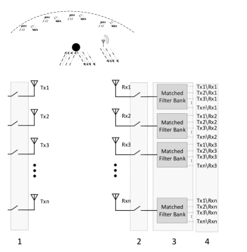
Figure 1: Block diagram of the considered MIMO system. Stage 1: transmit antenna selection. Stage 2: receive antenna selection. Stage 3: matched-filter selection in DSP. Stage 4: output signal selection.

By applying matched-filtering with respect to the $M$ orthogonal waveforms, the extended receive signal becomes

$$\tilde{\boldsymbol{x}}(\tau) =\mathrm{vec}\left(\int_{T_{p}}\textbf{x}(t,\tau)\boldsymbol{\phi}^{H}(t)dt\right)$$

$$=\tilde{\boldsymbol{x}}_{\mathrm{s}}(\tau)+\tilde{\boldsymbol{x}}_{\mathrm{c}}(\tau)+\tilde{\boldsymbol{x}}_{\mathrm{j}}(\tau)+\tilde{\boldsymbol{x}}_{\mathrm{n}}(\tau),$$

where $\tilde{\boldsymbol{x}}$ represents the vectorized version of the matched-filtered snapshot vector. Exploiting the orthogonality assumption, we can write the SOI as

$$\tilde{\boldsymbol{x}}_{\mathrm{s}}(\tau) =\beta_{s}\textbf{a}_{\mathrm{s}}$$

$$\textbf{a}_{\mathrm{s}} =\textbf{a}_{\mathrm{t}}(\theta_{\mathrm{t}})\otimes\textbf{a}_{\mathrm{r}}(\theta_{\mathrm{r}}),$$

where $\beta_{\mathrm{s}}$ is the target reflection coefficient, which we assume obeys the Swirling ii@ model. The transmit steering vector, $\textbf{a}_{\mathrm{t}}(\theta_{\mathrm{t}})$, corresponds the Direction-of-Departure (DoD) $\theta_{\mathrm{t}}$, and the receive steering vector, $\textbf{a}_{\mathrm{r}}(\theta_{\mathrm{r}})$, is associated with DoA $\theta_{\mathrm{r}}$. In the case of a ULA, the steering vectors are given by

$$\textbf{a}_{\mathrm{t}}(\theta_{\mathrm{t}}) =[1,e^{j2\pi d_{\mathrm{t}}sin\theta_{\mathrm{t}}},e^{j2\pi 2d_{\mathrm{t}}sin\theta_{\mathrm{t}}},...,e^{j2\pi Md_{\mathrm{t}}sin\theta_{\mathrm{t}}}],$$

$$\textbf{a}_{\mathrm{r}}(\theta_{\mathrm{r}}) =[1,e^{j2\pi d_{\mathrm{r}}sin\theta_{\mathrm{r}}},e^{j2\pi 2d_{\mathrm{r}}sin\theta_{\mathrm{r}}},...,e^{j2\pi Nd_{\mathrm{r}}sin\theta_{\mathrm{r}}}],$$

with $d_{\mathrm{t}},d_{\mathrm{r}}$ denoting the inter-element spacing employed in transmit and receive arrays.

Now assuming a set of angle cells, $\left\{\theta_{i}\right\}_{i=1}^{N_{\mathrm{c}}}$, we model the clutter as the reflections from these directions and extract the received clutter signal as

$$\tilde{\boldsymbol{x}}_{\mathrm{c}}(\tau) =\sum\limits_{i=1}^{N_{\mathrm{c}}}\beta_{i}\textbf{a}_{\mathrm{c},i}$$

$$\textbf{a}_{\mathrm{c},i} =\textbf{a}_{\mathrm{t}}(\theta_{\mathrm{tc},i})\otimes\textbf{a}_{\mathrm{r}}(\theta_{\mathrm{rc},i}),$$

where $\beta_{i}$ is the reflection coefficient of the $i$-th clutter cell from directions $\theta_{\mathrm{tc},i}$, and $\theta_{\mathrm{rc},i}$ with respect to transmit, and receive sides. Suppose that $N_{\mathrm{j}}$ jamming signals are in the field of view of the radar. Then the jamming signal is expressed as

$$\tilde{\boldsymbol{x}}_{\mathrm{j}}(\tau) =\sum\limits_{i=1}^{N_{\mathrm{j}}}\alpha_{i}\textbf{a}_{\mathrm{j},i}$$ (1)

$$\textbf{a}_{\mathrm{j},i} =\tilde{\boldsymbol{x}}_{\mathrm{j,i}}(\tau)\otimes\textbf{a}_{\mathrm{r}}(\theta_{\mathrm{rj},i}),$$ (2)

with $\alpha_{i}$, and $\tilde{\boldsymbol{x}}_{\mathrm{j,i}}(\tau)$ denoting the complex amplitude, and the matched filtered version of the $i$-th jamming signal. Given a strong jamming source $\textbf{x}_{\mathrm{j,i}}(t,\tau)$ with a power of $\hat{\alpha_{i}}$ , which emulates the radar orthogonal waveforms we have

$$\textbf{x}_{\mathrm{j,i}}(t,\tau)=\hat{\alpha_{i}}\sum\limits_{i=1}^{M}\phi_{i}(t,\tau),$$ (3)

then, this signal passes through the matched filters and by incorporating $\hat{\alpha_{i}}$ in $\alpha_{i}$ we can write $\tilde{\boldsymbol{x}}_{\mathrm{j,i}}(\tau)=\textbf{1}$ [Li2014, Vaidyanathan2009]. The received signal is then input to an adaptive filter with weights vector, w, giving the output

$$y(\tau)=\textbf{w}^{H}\tilde{\boldsymbol{x}}(\tau).$$ (4)

The weights vector that preserves the SOI, $\tilde{\boldsymbol{x}}_{\mathrm{s}}$, while suppressing the clutter, jammers and noise, thus maximizing the output SINR, is obtained by solving the following optimization

$$\min_{\textbf{w}}\; \textbf{w}^{H}\textbf{R}\textbf{w}$$ (5)

s.t. $$\textbf{w}^{H}\textbf{a}_{\mathrm{s}}=1.$$ (6)

This yields the solution [VanTrees2002]

$$\textbf{w}=\frac{\textbf{R}^{-1}\textbf{a}_{\mathrm{s}}}{\textbf{a}_{\mathrm{s}}^{H}\textbf{R}^{-1}\textbf{a}_{\mathrm{s}}},$$ (7)

where R is the interference (jamming and clutter) plus noise covariance matrix of size $MN\times MN$. Assuming the clutter, jammers and noise are statistically independent, we have

R $$=\textbf{R}_{\mathrm{c}}+\textbf{R}_{\mathrm{j}}+\textbf{R}_{n}.$$

Taking the clutter scattering coefficients, $\beta_{i}$ to be mutually uncorrelated, we find that

$$\textbf{R}_{\mathrm{c}} =\mathbb{E}\{\tilde{\boldsymbol{x}}_{\mathrm{c}}(\tau)\tilde{\boldsymbol{x}}^{H}_{\mathrm{c}}(\tau)\}=\sum\limits_{i=1}^{N_{\mathrm{c}}}\sigma^{2}_{\mathrm{c},i}\textbf{a}_{\mathrm{c},i}\textbf{a}_{\mathrm{c},i}^{H}=\textbf{A}_{\mathrm{c}}\textbf{P}_{\mathrm{c}}\textbf{A}_{\mathrm{c}}^{H},$$

where

$$\sigma^{2}_{\mathrm{c},i} =\mathbb{E}\{\beta_{i}\beta_{i}^{*}\},$$ (8)

$$\textbf{A}_{\mathrm{c}} =[a_{\mathrm{c},1},a_{\mathrm{c},2},...,a_{\mathrm{c},N_{\mathrm{c}}}],\;\;MN\times N_{\mathrm{c}}$$ (9)

and

$$\textbf{P}_{\mathrm{c}}=\mathrm{diag}\left(\sigma^{2}_{c,1},...,\sigma^{2}_{c,N_{\mathrm{c}}}\right).$$ (10)

Similarly, using (3), the covariance matrix for the jamming signal is found to be

$$\textbf{R}_{\mathrm{j}}=\mathbb{E}\{\tilde{\boldsymbol{x}}_{\mathrm{j}}(\tau)\tilde{\boldsymbol{x}}^{H}_{\mathrm{j}}(\tau)\}=\textbf{A}_{\mathrm{j}}\textbf{P}_{\mathrm{j}}\textbf{A}_{\mathrm{j}}^{H},$$

where $\textbf{A}_{\mathrm{j}}$, and $\textbf{P}_{\mathrm{j}}$ are $MN\times MN_{\mathrm{j}}$, and $MN_{\mathrm{j}}\times MN_{\mathrm{j}}$ matrices denoted as

$$\textbf{A}_{\mathrm{j}} =[\underbrace{\textbf{a}_{\mathrm{r}}(\theta_{{\mathrm{rj},1}}),...,\textbf{a}_{\mathrm{r}}(\theta_{{\mathrm{rj},1}})}_{M\;\mathrm{times}},...,\underbrace{\textbf{a}_{\mathrm{r}}(\theta_{{\mathrm{rj},N_{\mathrm{j}}}}),...,\textbf{a}_{\mathrm{r}}(\theta_{{\mathrm{rj},N_{\mathrm{j}}}})}_{M\;\mathrm{times}}],$$ (11)

$$\textbf{P}_{\mathrm{j}} =\mathrm{diag}(\underbrace{\sigma^{2}_{j,1},...,\sigma^{2}_{j,1}}_{M\;\mathrm{times}},...,\underbrace{\sigma^{2}_{j,N_{\mathrm{j}}},...,\sigma^{2}_{j,N_{\mathrm{j}}}}_{M\;\mathrm{times}}),$$ (12)

and

$$\sigma^{2}_{\mathrm{j},i}=\mathbb{E}\{\alpha_{i}\alpha_{i}^{*}\}.$$ (13)

Finally, the covariance matrix of the white noise is given by

$$\textbf{R}_{n} =\mathbb{E}\{\tilde{\boldsymbol{x}}_{\mathrm{n}}(\tau)\tilde{\boldsymbol{x}}^{H}_{\mathrm{n}}(\tau)\}=\sigma_{n}^{2}\textbf{I}_{MN}.$$

Now writing $\sigma^{2}_{\mathrm{s}}=\mathbb{E}\{\beta_{\mathrm{s}}\beta_{\mathrm{s}}^{*}\}$, the SINR at the output of the filter (7) is

$$\mathrm{SINR}_{\mathrm{out}}=\sigma^{2}_{\mathrm{s}}\textbf{a}_{\mathrm{s}}^{H}\textbf{R}^{-1}\textbf{a}_{\mathrm{s}}.$$ (14)

The inverse covariance matrix becomes

$$\textbf{R}^{-1} =\left(\textbf{A}_{\mathrm{c}}\textbf{P}_{\mathrm{c}}\textbf{A}_{\mathrm{c}}^{H}+\textbf{A}_{\mathrm{j}}\textbf{P}_{\mathrm{j}}\textbf{A}_{\mathrm{j}}^{H}+\sigma_{n}^{2}\textbf{I}_{MN}\right)^{-1}$$ (15)

$$\stackrel{{\scriptstyle\text{(a)}}}{{=}}\left(\textbf{A}_{\mathrm{jc}}\textbf{P}_{\mathrm{jc}}\textbf{A}_{\mathrm{jc}}^{H}+\sigma_{n}^{2}\textbf{I}_{MN}\right)^{-1}$$ (16)

$$\stackrel{{\scriptstyle\text{(b)}}}{{=}}\sigma^{-2}_{n}\left(I_{MN}-\textbf{A}_{\mathrm{jc}}\left(\sigma^{2}_{n}\textbf{P}_{\mathrm{\mathrm{jc}}}^{-1}+\textbf{A}_{\mathrm{jc}}^{H}\textbf{A}_{\mathrm{jc}}\right)^{-1}\textbf{A}_{\mathrm{jc}}^{H}\right),$$ (17)

where in (a) we put $\textbf{A}_{\mathrm{jc}}=[\textbf{A}_{\mathrm{c}},\textbf{A}_{\mathrm{j}}]$, and $\textbf{P}_{\mathrm{jc}}=\mathrm{diag}\left(\textbf{P}_{\mathrm{c}},\textbf{P}_{\mathrm{j}}\right)$, and (b) follows from the matrix inversion lemma. Now, we can reformulate the output SINR as

$$\mathrm{SINR}_{\mathrm{out}} =\frac{\sigma^{2}_{s}}{\sigma^{2}_{n}}\textbf{a}_{s}^{H}\big{(}\textbf{I}_{MN}-\textbf{A}_{\mathrm{jc}}(\sigma^{2}_{n}\textbf{P}_{\mathrm{jc}}^{-1}+\textbf{A}_{\mathrm{jc}}^{H}\textbf{A}_{\mathrm{jc}})^{-1}\textbf{A}_{\mathrm{jc}}^{H}\big{)}\textbf{a}_{s}.$$ (18)

Defining the matrices

$$\textbf{B}_{\mathrm{jc}}=\sigma_{n}^{2}\textbf{P}_{\mathrm{jc}}^{-1},\;\;\textbf{A}_{\mathrm{s}}=[\textbf{a}_{s},\textbf{A}_{\mathrm{jc}}],\;\;\textbf{B}_{\mathrm{s}}=\left[\textbf{0},\sigma_{n}^{2}\textbf{P}_{\mathrm{jc}}^{-1}\right],$$ (19)

and making use of the determinant formula of block matrices, we obtain[Wang2016, Deligiannis2018]

$$\left|\textbf{A}_{\mathrm{s}}^{H}\textbf{A}_{\mathrm{s}}+\textbf{B}_{\mathrm{s}}\right| =\left|\begin{matrix}\textbf{a}_{s}^{H}\textbf{a}_{s}&\textbf{a}_{s}^{H}\textbf{A}_{\mathrm{jc}}\\ \textbf{A}_{\mathrm{jc}}^{H}\textbf{a}_{s}&\textbf{A}_{\mathrm{jc}}^{H}\textbf{A}_{\mathrm{jc}}+\textbf{B}_{\mathrm{jc}}\\ \end{matrix}\right|$$

$$=\left|\textbf{A}_{\mathrm{jc}}^{H}\textbf{A}_{\mathrm{jc}}+\textbf{B}_{\mathrm{jc}}\right|$$

$$\times \textbf{a}_{s}^{H}\left(\textbf{I}_{MN}-\textbf{A}_{\mathrm{jc}}\left(\textbf{B}_{\mathrm{jc}}+\textbf{A}_{\mathrm{jc}}^{H}\textbf{A}_{\mathrm{jc}}\right)^{-1}\textbf{A}_{\mathrm{jc}}^{H}\right)\textbf{a}_{s}.$$ (20)

Substituting this into the expression of $\mathrm{SINR}_{out}$ yields

$$\mathrm{SINR}_{\mathrm{out}} =\frac{\sigma^{2}_{s}}{\sigma^{2}_{n}}\frac{\left|\textbf{A}_{\mathrm{s}}^{H}\textbf{A}_{\mathrm{s}}+\textbf{B}_{\mathrm{s}}\right|}{\left|\textbf{A}_{\mathrm{jc}}^{H}\textbf{A}_{\mathrm{jc}}+\textbf{B}_{\mathrm{jc}}\right|},$$

where $\left|.\right|$ denotes the determinant and the signal-to-noise ratio, $\mathrm{SNR}=\frac{\sigma^{2}_{s}}{\sigma^{2}_{n}}$. This reveals that, although the SNR is constant, the set of active transmit and receive elements directly affects the achieved output SINR by varying the interplay among the jamming and clutter steering vectors and their powers. Let us introduce a binary vector c with elements 0 if their corresponding elements are inactive and 1 otherwise. Then the element selection can be incorporated into the expression of the output $\mathrm{SINR}$ as follows

$$\mathrm{SINR}_{\mathrm{out}}(\textbf{c})=\frac{\sigma^{2}_{s}}{\sigma^{2}_{n}}h(\textbf{c}),$$ (21)

where

$$h(\textbf{c})=\frac{\left|\textbf{A}_{\mathrm{s}}^{H}\mathrm{diag}(\textbf{c})\textbf{A}_{\mathrm{s}}+\textbf{B}_{\mathrm{s}}\right|}{\left|\textbf{A}_{\mathrm{jc}}^{H}\mathrm{diag}(\textbf{c})\textbf{A}_{\mathrm{jc}}+\textbf{B}_{\mathrm{jc}}\right|}.$$ (22)

The optimum set of $k$ active elements that maximizes the SINR is found via the following optimization:

$$\max_{\textbf{c}}\,\, \mathrm{SINR}_{\mathrm{out}}(\textbf{c})$$ (23)

$$\mathrm{s.t.}\,\, c_{i}^{2}-c_{i}=0\,\,\,\,\,i=1...MN,$$ (24)

$$\textbf{c}^{T}\textbf{c}=k.$$ (25)

The optimization in (23) is maximization of the volume of two ellipsoids. Therefore, we may employ log-determinant function as

$$f(\textbf{c})= \mathrm{logdet}\left(h\left(\textbf{c}\right)\right)$$

$$= \mathrm{logdet}\left(\textbf{A}_{\mathrm{s}}^{H}\mathrm{diag}(\textbf{c})\textbf{A}_{\mathrm{s}}+\textbf{B}_{\mathrm{s}}\right)$$

$$-\mathrm{logdet}\left(\textbf{A}_{\mathrm{jc}}^{H}\mathrm{diag}(\textbf{c})\textbf{A}_{\mathrm{jc}}+\textbf{B}_{\mathrm{jc}}\right).$$ (26)

This problem can be effectively solved via a log-determinant relaxation and a sequential convex programming (SCP) procedure accordingly. We will elaborate on the solution approximation in Section LABEL:sec:relaxation.

Considering (23), we propose four different methods to apply selection in a MIMO radar. We list all the requirements in different modes in a quadratic form. Hence, we cast the general problem of antenna selection in a MIMO radar as follows

$$\max_{\textbf{c}}\,\, f(\textbf{c})$$ (27)

$$\textbf{c}^{T}\textbf{W}_{i}\textbf{c}+\textbf{q}_{i}^{T}\textbf{c}+r_{i}\leq 0,\;\;\;\;i=1,...,\ell.$$ (28)

where $\textbf{W}_{i}\in\mathbb{S}^{MN}$, $\textbf{q}_{i}\in\mathbb{R}^{MN}$, and $r_{i}\in\mathbb{R}$. Note that $\mathbb{S}^{n}$ denotes the set of $n\times n$ symmetric matrices, and $\mathbb{R}^{n}$ represents the set of real vectors of size $n$.

III Selection strategies

The selection strategy may be applied at each of the four stages of a MIMO radar depicted in Fig. 1. In what follows, we detail and compare these selection approaches.

III-A Joint Tx-Rx selection

The first selection strategy involves thinning the MIMO virtual array by selecting the individual matched-filters at the output (stage 4) of Fig. 1. In this case, we reshape the selection vector c as a matrix C

$$\textbf{C}=\bordermatrix{~{}&\text{Tx}_{1}&\text{Tx}_{2}&\cdots&\text{Tx}_{M}\cr\text{Rx}_{1}&c_{1,1}&c_{1,2}&\cdots&c_{1,M}\cr\text{Rx}_{2}&c_{2,1}&c_{2,2}&\cdots&c_{2,M}\cr\vdots&\vdots&\vdots&\ddots&\vdots\cr\text{Rx}_{N}&c_{N,1}&c_{N,2}&\cdots&c_{N,M}\cr},$$ (29)

such that $\textbf{c}=\mathrm{vec}(\textbf{C})$, and $c_{i,j}$ is the entry that indicates whether the $j$-th matched filter (which extracts the $j$-th waveform) in the $i$-th receiver is selected. The joint thinning mode is obtained by directly selecting $k$ elements in c. The selection problem of (27) can now be written as

$$\max_{\textbf{c}}\,\, f(\textbf{c})$$

$$\mathrm{s.t.}\,\, c_{i}^{2}-c_{i}=0\,\,\,\,\,i=1...MN,$$

$$\textbf{c}^{T}\textbf{c}=k.$$ (30)

In this formulation, we place a constraint only on the number of output signals and any subset of the output matched filters is a possible solution. The joint selection finds the best subset, which decreases the dimensionality of the signal used in the post processing (e.g. for detection, estimation or other tasks). However, the entire system including transmitters, receivers, and matched filters should be active, and consequently the hardware cost and power consumption remain high.

III-B Factored Tx and Rx selection

As all of the transmitters are required to be active in the joint selection strategy, transmitters that do not contribute to the selected set of matched-filters effectively waste the power alloted to them. This issue can be mitigated by factorizing the selection problem into transmit and receive sub-problems. Suppose that we select $k_{\mathrm{t}}$ out of $M$ transmitting antennas (stage 1 in Fig. 1) and $k_{\mathrm{r}}$ out of the available $N$ receive antennas (stage 2 in Fig. 1). In terms of the selection matrix (29), this strategy selects $k_{\mathrm{r}}$ rows and $k_{\mathrm{t}}$ columns. Then the factored selection involves the optimization of two selection vectors jointly, one for the transmitters and the other for the receivers. We now develop a novel way to reformulate this coupled problem in one unified formulation.

Let $\textbf{V}_{\mathrm{t}}=\{\textbf{v}_{\mathrm{t},1},...,\textbf{v}_{\mathrm{t},M}\}$, and $\textbf{V}_{\mathrm{r}}=\{\textbf{v}_{\mathrm{r},1},...,\textbf{v}_{\mathrm{r},N}\}$ be a set of binary vectors each of which denoting a specific transmitter or receiver in the selection matrix

$$\textbf{v}_{\mathrm{t},i} =\mathrm{vec}\left(\left[\textbf{0},\ldots,\underset{\text{Tx}_{i}}{\textbf{1}},\ldots,\textbf{0}\right]\right)$$ (31)

$$\textbf{v}_{\mathrm{r},i} =\mathrm{vec}\left(\left[\textbf{0},\ldots,\underset{\text{Rx}_{i}}{\textbf{1}},\ldots,\textbf{0}\right]^{T}\right)$$ (32)

Then, the factored selection problem may be expressed as

max_c  & f(c)
s.t.   c_i^2-c_i=0      i=1…MN,
   c^TP_t,ic∈{0,k_r}      i=1…M,
   c^TP_r,ic∈{0,k_t}      i=1…N,
  c^Tc=k_t k_r,

where

$$\textbf{P}_{{\mathrm{t},i}}=\text{diag}(\textbf{v}_{\mathrm{t},i}),i=1,...,M,\;\textbf{P}_{{\mathrm{r},i}}=\text{diag}(\textbf{v}_{\mathrm{r},i}),i=1,...,N.$$ (35)

In (34) and (34) we constrain the number of active elements in each column (row) to be exactly 0 or $k_{\mathrm{t}}$ (0 or $k_{\mathrm{r}}$).

Now let us define Q as the rectangular matrix

Q $$=\textbf{P}\textbf{P}^{T},\text{ where}\;\;\textbf{P}=\left[\textbf{v}_{\mathrm{t},1},...,\textbf{v}_{\mathrm{t},M},\textbf{v}_{\mathrm{r},1},...,\textbf{v}_{\mathrm{r},N}\right].$$ (36)

Theorem 1

Let $\mathcal{S}$ be the set of selection vectors in conjunction with a factored selection problem comprising of $k_{\mathrm{t}}$ and $k_{\mathrm{r}}$ out of $M$ transmitters and $N$ receivers respectively. Then $\mathcal{S}$ is given by

$$\mathcal{S}=\mathcal{S}_{1}\cap\mathcal{S}_{2}\cap\mathcal{S}_{3}\cap\mathcal{S}_{4},$$

where the sets $\mathcal{S}_{1}$ - $\mathcal{S}_{4}$ are defined as

$$\mathcal{S}_{1}=\{\textbf{c}\;|\;\textbf{c}^{T}\textbf{Q}\textbf{c}=k_{\mathrm{r}}k_{\mathrm{t}}(k_{\mathrm{r}}+k_{\mathrm{t}})\}$$

$$\mathcal{S}_{2}=\{\textbf{c}\;|\;\textbf{c}^{T}\textbf{P}_{{\mathrm{t},i}}\textbf{c}\leq k_{\mathrm{r}}\,\,\,\,\,i=1...M,\}$$

$$\mathcal{S}_{3}=\{\textbf{c}\;|\;\textbf{c}^{T}\textbf{P}_{{\mathrm{r},i}}\textbf{c}\leq k_{\mathrm{t}}\,\,\,\,\,i=1...N\}$$

$$\mathcal{S}_{4}=\{\textbf{c}\;|\;\textbf{c}^{T}\textbf{c}=k_{\mathrm{t}}k_{\mathrm{r}}\}.$$

Proof: See Appendix LABEL:sec:appendix_Proof_theorem1.

Like the constraint in (34), the binary constraints involving the quadratic forms in (34) and (34) are non-convex. Therefore, we propose relaxing them by employing the following set of quadratic constraints instead

$$\textbf{c}^{T}\textbf{Q}\textbf{c} =k_{\mathrm{r}}k_{\mathrm{t}}(k_{\mathrm{r}}+k_{\mathrm{t}})$$ (37)

$$\textbf{c}^{T}\textbf{P}_{{\mathrm{t},i}}\textbf{c} \leq k_{\mathrm{r}}\,\,\,\,\,i=1...M$$ (38)

$$\textbf{c}^{T}\textbf{P}_{{\mathrm{r},i}}\textbf{c} \leq k_{\mathrm{t}}\,\,\,\,\,i=1...N,$$ (39)

Using Theorem 1, the factored selection problem becomes

max_c  & f(c)
s.t.   c_i(c_i-1)=0      i=1…MN,
c^Tc=k_tk_r
c^TQc= k_rk_t (k_r+k_t )
c^TP_t,ic≤k_r       i=1…M,
c^TP_r,ic≤k_t       i=1…N.

We recast the added binary constraints in the factored problem, into a quadratic form as a special case of (27). This enables us to compare the performance of the factored selection with that of the joint selection. We show that the optimum solution (i.e. SINR) obtained by the Lagrange dual of the joint selection optimization is always greater than or equal to that yielded by the factored problem. To this end, we derive a dual problem for the factored selection problem in (40). We revise the factored problem (40), by introducing new variables X, and Y as

min_c  & log det(X^-1)-log det(Y^-1)
s.t.
Λ: X=A_s^H diag(c) A_s+B_s
Δ: Y=A_jc^H diag(c) A_jc+B_jc
μ_i:    c_i(c_i-1)=0      i=1…MN,
ν:   c^Tc=k_tk_r
λ:   c^TQc≤k_rk_t (k_r+k_t)
ρ_i: c^TP_t,ic≤k_r      i=1…M,
η_i: c^TP_r,ic≤k_t       i=1…N,

with Lagrange multipliers $\boldsymbol{\Lambda}\in\mathbb{S}^{n+1}(n=N_{\mathrm{c}}+N_{\mathrm{j}})$, $\boldsymbol{\Delta}\in\mathbb{S}^{n}$, $\boldsymbol{\mu}\in\mathbb{R}^{MN}$, $\boldsymbol{\rho}\in\mathbb{R}^{M}$, $\boldsymbol{\eta}\in\mathbb{R}^{N}$, and $\nu,\lambda\in\mathbb{R}$. We then introduce the Lagrangian

$$L^{\mathrm{fct}}( \textbf{c},\textbf{X},\textbf{Y},\boldsymbol{\Lambda},\boldsymbol{\Delta},\boldsymbol{\mu},\nu,\lambda,\boldsymbol{\rho},\boldsymbol{\eta})=$$

$$\mathrm{logdet}(\textbf{X}^{-1})-\mathrm{logdet}(\textbf{Y}^{-1})+\mathrm{tr}(\textbf{X}\boldsymbol{\Lambda})+\mathrm{tr}(\textbf{Y}\boldsymbol{\Delta})$$

$$+\textbf{c}^{T}(\text{diag}(\boldsymbol{\mu})+\nu\textbf{I}+\lambda\textbf{Q}+\sum\limits_{i=1}^{M}\rho_{i}\textbf{P}_{t,i}+\sum\limits_{i=1}^{N}\eta_{i}\textbf{P}_{r,i})\textbf{c}$$

$$-\boldsymbol{\Lambda}\left(\textbf{A}_{\mathrm{s}}^{H}\mathrm{diag}(\textbf{c})\textbf{A}_{\mathrm{s}}+\textbf{B}_{\mathrm{s}}\right)-\boldsymbol{\Delta}\left(\textbf{A}_{\mathrm{jc}}^{H}\mathrm{diag}(\textbf{c})\textbf{A}_{\mathrm{jc}}+\textbf{B}_{\mathrm{jc}}\right)$$

$$-\boldsymbol{\mu}^{T}\textbf{c}-k_{\mathrm{t}}k_{\mathrm{r}}\nu-\lambda k_{\mathrm{r}}k_{\mathrm{t}}(k_{\mathrm{r}}+k_{\mathrm{t}})$$

$$-k_{\mathrm{r}}\sum\limits_{i=1}^{M}\rho_{i}-k_{\mathrm{t}}\sum\limits_{i=1}^{N}\eta_{i}.$$ (42)

By rearranging the Lagrangian we get

$$L^{\mathrm{fct}}( \textbf{c},\textbf{X},\textbf{Y},\boldsymbol{\Lambda},\boldsymbol{\Delta},\boldsymbol{\mu},\nu,\lambda,\boldsymbol{\rho},\boldsymbol{\eta})=$$

$$\mathrm{logdet}(\textbf{X}^{-1})-\mathrm{logdet}(\textbf{Y}^{-1})+\mathrm{tr}(\textbf{X}\boldsymbol{\Lambda})+\mathrm{tr}(\textbf{Y}\boldsymbol{\Delta})$$

$$-\mathrm{tr}(\textbf{B}_{\mathrm{s}}\boldsymbol{\Lambda})-\mathrm{tr}(\textbf{B}_{\mathrm{jc}}\boldsymbol{\Delta})$$

$$+ \sum\limits_{i=1}^{MN}c_{i}\underbrace{\left(\left[\textbf{A}_{\mathrm{s}}^{T}\right]_{i}^{T}\boldsymbol{\Lambda}\left[\textbf{A}_{\mathrm{s}}^{H}\right]_{i}+\left[\textbf{A}_{\mathrm{jc}}^{T}\right]_{i}^{T}\boldsymbol{\Delta}\left[\textbf{A}_{\mathrm{jc}}^{H}\right]_{i}+\mu_{i}\right)}_{\omega_{i}}$$

$$+\textbf{c}^{T}(\text{diag}(\boldsymbol{\mu})+\nu\textbf{I}+\lambda\textbf{Q}+\sum\limits_{i=1}^{M}\rho_{i}\textbf{P}_{t,i}+\sum\limits_{i=1}^{N}\eta_{i}\textbf{P}_{r,i})\textbf{c}$$

$$-k_{\mathrm{t}}k_{\mathrm{r}}\nu-\lambda k_{\mathrm{r}}k_{\mathrm{t}}(k_{\mathrm{r}}+k_{\mathrm{t}})$$

$$-N\sum\limits_{i=1}^{M}\rho_{i}+M\sum\limits_{i=1}^{N}\eta_{i}.$$ (43)

We minimize $L^{\mathrm{fct}}$ with respect to c, X, and Y. Noting that $L^{\mathrm{fct}}$ is a mixture of two volume covering ellipsoids in terms of X, and Y (see p 222 in [Boyd2010b], and Appendix in [Joshi2009]) and given the set of quadratic forms in c, we arrive at the Lagrange dual function $g^{\mathrm{fct}}$ in (48).

$$g^{\mathrm{fct}}(\boldsymbol{\Lambda},\boldsymbol{\Delta},\boldsymbol{\mu},\nu,\lambda,\boldsymbol{\rho},\boldsymbol{\eta})=\inf_{\textbf{c},\textbf{X},\textbf{Y}}L^{\mathrm{fct}}(\textbf{c},\textbf{X},\textbf{Y},\boldsymbol{\Lambda},\boldsymbol{\Delta},\boldsymbol{\mu},\nu,\lambda,\boldsymbol{\rho},\boldsymbol{\eta})\}$$

$$=\left\{\begin{array}[]{llll}\mathrm{logdet}(\boldsymbol{\Lambda})+\mathrm{logdet}(\boldsymbol{\Delta})+2n+1-\mathrm{tr}(\boldsymbol{\Lambda}\textbf{B}_{\mathrm{s}})-\mathrm{tr}(\boldsymbol{\Delta}\textbf{B}_{\mathrm{jc}})-\frac{1}{4}\boldsymbol{\omega}^{T}\bigg{(}\text{diag}(\boldsymbol{\mu})+\nu\textbf{I}+\lambda\textbf{Q}+\sum\limits_{i=1}^{M}\rho_{i}\textbf{P}_{t,i}+\sum\limits_{i=1}^{N}\eta_{i}\textbf{P}_{r,i}\bigg{)}^{-1}\boldsymbol{\omega}\\ \hskip 256.0748pt-k_{\mathrm{t}}k_{\mathrm{r}}\nu-\lambda k_{\mathrm{r}}k_{\mathrm{t}}(k_{\mathrm{r}}+k_{\mathrm{t}})-k_{\mathrm{r}}\sum\limits_{i=1}^{M}\rho_{i}-k_{\mathrm{t}}\sum\limits_{i=1}^{N}\eta_{i}\\ \hskip 142.26378pt\text{if}\;\;\bigg{(}\text{diag}(\boldsymbol{\mu})+\nu\textbf{I}+\lambda\textbf{Q}+\sum\limits_{i=1}^{M}\rho_{i}\textbf{P}_{t,i}+\sum\limits_{i=1}^{N}\eta_{i}\textbf{P}_{r,i}\bigg{)}\succeq 0,\textbf{X}\succeq 0,\textbf{Y}\succeq 0\\ -\infty\;\;\;\;\;\;\;\text{otherwise.}\end{array}\right.$$ (48)

$$g^{\mathrm{jnt}}(\boldsymbol{\Lambda},\boldsymbol{\Delta},\boldsymbol{\mu},\nu,\lambda,\boldsymbol{\rho},\boldsymbol{\eta})=\inf_{\textbf{c},\textbf{X},\textbf{Y}}L^{\mathrm{jnt}}(\textbf{c},\textbf{X},\textbf{Y},\boldsymbol{\Lambda},\boldsymbol{\Delta},\boldsymbol{\mu},\nu,\lambda,\boldsymbol{\rho},\boldsymbol{\eta})\}$$

$$=\left\{\begin{array}[]{llll}\mathrm{logdet}(\boldsymbol{\Lambda})+\mathrm{logdet}(\boldsymbol{\Delta})+2n+1-\mathrm{tr}(\boldsymbol{\Lambda}\textbf{B}_{\mathrm{s}})-\mathrm{tr}(\boldsymbol{\Delta}\textbf{B}_{\mathrm{jc}})-\frac{1}{4}\boldsymbol{\omega}^{T}\bigg{(}\text{diag}(\boldsymbol{\mu})+\nu\textbf{I}+\lambda\textbf{Q}+\sum\limits_{i=1}^{M}\rho_{i}\textbf{P}_{t,i}+\sum\limits_{i=1}^{N}\eta_{i}\textbf{P}_{r,i}\bigg{)}^{-1}\boldsymbol{\omega}\\ \hskip 256.0748pt-k^{\mathrm{jnt}}\nu-\lambda k^{\mathrm{jnt}}(M+N)-N\sum\limits_{i=1}^{M}\rho_{i}-M\sum\limits_{i=1}^{N}\eta_{i}\\ \hskip 142.26378pt\text{if}\;\;\bigg{(}\text{diag}(\boldsymbol{\mu})+\nu\textbf{I}+\lambda\textbf{Q}+\sum\limits_{i=1}^{M}\rho_{i}\textbf{P}_{t,i}+\sum\limits_{i=1}^{N}\eta_{i}\textbf{P}_{r,i}\bigg{)}\succeq 0,\textbf{X}\succeq 0,\textbf{Y}\succeq 0\\ -\infty\;\;\;\;\;\;\;\text{otherwise.}\end{array}\right.$$ (48)

Theorem 2

Let $f^{\text{jnt}}$ be the optimal value associated with the joint selection (23) and $f^{\text{fct}}$ be that of the factored selection (40). Also, let $k_{\mathrm{r}}^{\mathrm{fct}}$, $k_{\mathrm{t}}^{\mathrm{fct}}$ be the number of selected transmitters and receivers in the factored selection, and $k^{\mathrm{jnt}}$ the number of jointly selected elements such that $k^{\mathrm{jnt}}=k_{\mathrm{r}}^{\mathrm{fct}}k_{\mathrm{t}}^{\mathrm{fct}}$. Then

$$f^{\text{jnt}}\geq f^{\text{fct}}.$$ (49)

Proof:

Let us recast the joint problem as

max_c  & f(c)
s.t.
μ_i:    c_i(c_i-1)=0      i=1…MN,
ν:   c^Tc=k^jnt
λ:   c^TQc≤k^jnt (M+N)
ρ_i: c^TP_t,ic≤N      i=1…M,
η_i: c^TP_r,ic≤M       i=1…N,

We can also reformulate (50) in terms of the equivalent minimization like (41) and derive the Lagrange dual function $g^{\mathrm{jnt}}$ as in (48). By minimization reformulation and employing $\bar{f}^{\text{jnt}}$, and $\bar{f}^{\text{fct}}$ as the corresponding optimal values, the expression in (49) can be transformed into

$$\bar{f}^{\text{jnt}}\leq\bar{f}^{\text{fct}}.$$ (51)

Given the upper bounds in (48) and (48), we show (49) by equivalently proving that

$$g^{\mathrm{jnt}}\leq g^{\mathrm{fct}}.$$ (52)

Now we have that

$$\textbf{Q}\succeq 0,\;\;\textbf{P}_{t,i}\succeq 0,i=1,...,M \;,\;\;\textbf{P}_{r,i}\succeq 0,i=1,...,N.$$ (53)

Also, the Karush-Kuhn-Tucker (KKT) conditions [Boyd2010b] imply that

$$\lambda\geq 0,\;\;\boldsymbol{\rho}\geq 0,\;\;\boldsymbol{\eta}\geq 0.$$ (54)

Therefore, by subtracting (48) and (48) we get

$$g^{\text{fct}}-g^{\text{jnt}} =\lambda\Big{(}k^{\mathrm{jnt}}\big{(}(M+N)-(k_{\mathrm{r}}^{\mathrm{fct}}+k_{\mathrm{t}}^{\mathrm{fct}})\big{)}\Big{)}$$

$$\quad+\sum\limits_{i=1}^{M}\rho_{i}\left(N-k_{\mathrm{r}}^{\mathrm{fct}}\right)+\sum\limits_{i=1}^{N}\eta_{i}\left(M-k_{\mathrm{t}}^{\mathrm{fct}}\right)$$ (55)

$$\geq 0$$

∎

The factored selection operates on a subset of solutions that is included in the joint selection, and hence may not achieve the same optimal solution that is guaranteed by joint selection. Nonetheless, selecting a subset of transmitters allows the available total transmit power to be allocated only to the chosen elements. This is in contrast to the joint selection problem where all transmitters must be operational to guarantee that all matched filters are available for selection. Thus, assuming a total available transmit power $P_{e}=P_{T}$, the transmit power per element in the factored case is $P_{e}=\frac{P_{t}}{k_{\mathrm{t}}}$ as opposed to $\frac{P_{t}}{M}$ for the joint selection case. It is important to note, however that increasing the allocation of transmit power per element may be restricted by the hardware limitations of the components in the RF chain, such as amplifier linear range. This may limit the gain achievable by the factored approach.

III-C Matched Filter Constrained Selection

We can adjust the transmitter power and SNR by a factored selection. Moreover, the number of receivers is decreased, which leads to a considerable hardware reduction. Since the number of transmitters is reduced in a factored selection, the spatial diversity is reduced significantly[Nosrati2017c]. To preserve the spatial diversity provided by MIMO arrays but still reduce hardware and computation overheads, we propose restricting the number of matched filters in each receiver, as well as the number of receivers, in a matched filter constrained (MFC) selection strategy [Nosrati2017]. Using this, we decrease the number of RF front-ends on the receive end (stage 2 in Fig.1) as well as the required processing blocks in DSP (stage 3 in Fig.1).

We specify the MFC selection to select $k_{\mathrm{m}}$ matched filters in $k_{\mathrm{r}}$ receivers as follows

max_c  & f(c)
s.t.   c_i^2-c_i=0      i=1…MN,
c^Tc=k_mk_r,
c^TQ_rc=k_m^2 k_r,
c^TP_t,ic¡=k_r      i=1…M,
c