capbtabboxtable[][\FBwidth] \newfloatcommandcapbalgboxalgorithm[][\FBwidth]
Reducing Noise in GAN Training with Variance Reduced Extragradient
Abstract
We study the effect of the stochastic gradient noise on the training of generative adversarial networks (GANs) and show that it can prevent the convergence of standard game optimization methods, while the batch version converges. We address this issue with a novel stochastic variance-reduced extragradient (SVRE) optimization algorithm, which for a large class of games improves upon the previous convergence rates proposed in the literature. We observe empirically that SVRE performs similarly to a batch method on MNIST while being computationally cheaper, and that SVRE yields more stable GAN training on standard datasets.
1 Introduction
Many empirical risk minimization algorithms rely on gradient-based optimization methods. These iterative methods handle large-scale training datasets by computing gradient estimates on a subset of it, a mini-batch, instead of using all the samples at each step, the full batch, resulting in a method called stochastic gradient descent (SGD, Robbins and Monro (1951); Bottou (2010)).
SGD methods are known to efficiently minimize single objective loss functions, such as cross-entropy for classification or squared loss for regression. Some algorithms go beyond such training objective and define multiple agents with different or competing objectives. The associated optimization paradigm requires a multi-objective joint minimization. An example of such a class of algorithms are the generative adversarial networks (GANs, Goodfellow et al., 2014), which aim at finding a Nash equilibrium of a two-player minimax game, where the players are deep neural networks (DNNs).
As of their success on supervised tasks, SGD based algorithms have been adopted for GAN training as well. Recently, Gidel et al. (2019a) proposed to use an optimization technique coming from the variational inequality literature called extragradient (Korpelevich, 1976) with provable convergence guarantees to optimize games (see § 2). However, convergence failures, poor performance (sometimes referred to as “mode collapse”), or hyperparameter susceptibility are more commonly reported compared to classical supervised DNN optimization.
We question naive adoption of such methods for game optimization so as to address the reported training instabilities. We argue that as of the two player setting, noise impedes drastically more the training compared to single objective one. More precisely, we point out that the noise due to the stochasticity may break the convergence of the extragradient method, by considering a simplistic stochastic bilinear game for which it provably does not converge.
The theoretical aspect we present in this paper is further supported empirically, since using larger mini-batch sizes for GAN training has been shown to considerably improve the quality of the samples produced by the resulting generative model: Brock et al. (2019) report a relative improvement of of the Inception Score metric (see § 4) on ImageNet if the batch size is increased –fold. This notable improvement raises the question if noise reduction optimization methods can be extended to game settings. In turn, this would allow for a principled training method with the practical benefit of omitting to empirically establish this multiplicative factor for the batch size.
In this paper, we investigate the interplay between noise and multi-objective problems in the context of GAN training. Our contributions can be summarized as follows: (i) we show in a motivating example how the noise can make stochastic extragradient fail (see § 2.2). (ii) we propose a new method “stochastic variance reduced extragradient” (SVRE) that combines variance reduction and extrapolation (see Alg. 1 and § 3.2) and show experimentally that it effectively reduces the noise. (iii) we prove the convergence of SVRE under local strong convexity assumptions, improving over the known rates of competitive methods for a large class of games (see § 3.2 for our convergence result and Table 1 for comparison with standard methods). (iv) we test SVRE empirically to train GANs on several standard datasets, and observe that it can improve SOTA deep models in the late stage of their optimization (see § 4).
| Method | Complexity | -adaptivity |
|---|---|---|
| SVRG | no | |
| Acc. SVRG | no | |
| SVRE §3.2 | if |
2 GANs as a Game and Noise in Games
2.1 Game theory formulation of GANs
The models in a GAN are a generator , that maps an embedding space to the signal space, and should eventually map a fixed noise distribution to the training data distribution, and a discriminator whose purpose is to allow the training of the generator by classifying genuine samples against generated ones. At each iteration of the algorithm, the discriminator is updated to improve its “real vs. generated” classification performance, and the generator to degrade it.
From a game theory point of view, GAN training is a differentiable two-player game where the generator and the discriminator aim at minimizing their own cost function and , resp.:
| (2P-G) |
When this game is called a zero-sum game and (2P-G) is a minimax problem:
| (SP) |
The gradient method does not converge for some convex-concave examples (Mescheder et al., 2017; Gidel et al., 2019a). To address this, Korpelevich (1976) proposed to use the extragradient method111For simplicity, we focus on unconstrained setting where . For the constrained case, a Euclidean projection on the constraints set should be added at every update of the method. which performs a lookahead step in order to get signal from an extrapolated point:
| (EG) |
Note how and are updated with a gradient from a different point, the extrapolated one. In the context of a zero-sum game, for any convex-concave function and any closed convex sets and , the extragradient method converges (Harker and Pang, 1990, Thm. 12.1.11).
2.2 Stochasticity Breaks Extragradient
[\capbeside\thisfloatsetupcapbesideposition=right,top,capbesidewidth=6.8cm]figure[\FBwidth]
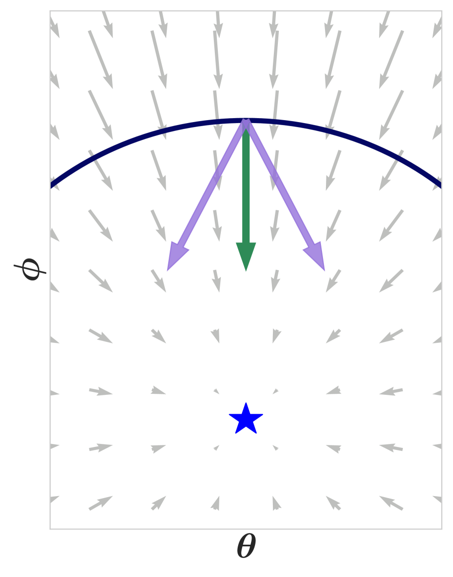
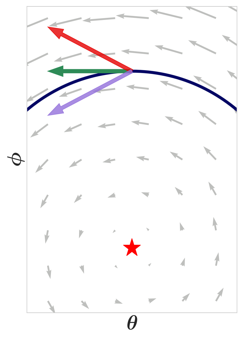
As the (EG) converges for some examples for which gradient methods do not, it is reasonable to expect that so does its stochastic counterpart (at least to a neighborhood). However, the resulting noise in the gradient estimate may interact in a problematic way with the oscillations due to the adversarial component of the game222Gidel et al. (2019b) formalize the notion of “adversarial component” of a game, which yields a rotational dynamics in gradients methods (oscillations in parameters), as illustrated by the gradient field of Fig. 1 (right).. We depict this phenomenon in Fig. 1, where we show the direction of the noisy gradient on single objective minimization example and contrast it with a multi-objective one.
We present a simplistic example where the extragradient method converges linearly (Gidel et al., 2019a, Corollary 1) using the full gradient but diverges geometrically when using stochastic estimates of it. Note that standard gradient methods, both batch and stochastic, diverge on this example.
In particular, we show that: (i) if we use standard stochastic estimates of the gradients of with a simple finite sum formulation, then the iterates produced by the stochastic extragradient method (SEG) diverge geometrically, and on the other hand (ii) the full-batch extragradient method does converge to the Nash equilibrium of this game (Harker and Pang, 1990, Thm. 12.1.11).
Theorem 1 (Noise may induce divergence).
For any There exists a zero-sum -strongly monotone stochastic game such that if , then for any step-size , the iterates computed by the stochastic extragradient method diverge geometrically, i.e., there exists such that .
Proof sketch. All detailed proofs can be found in § C of the appendix. We consider the following stochastic optimization problem (with ):
| (1) |
Note that this problem is a simple dot product between and with an - norm penalization, thus we can compute the batch gradient and notice that the Nash equilibrium of this problem is . However, as we shall see, this simple problem breaks with standard stochastic optimization methods.
Sampling a mini-batch without replacement , we denote . The extragradient update rule can be written as:
| (2) |
where and are the mini-batches sampled for the update and the extrapolation step, respectively. Let us write . Noticing that if and otherwise, we have,
| (3) |
Consequently, if the mini-batch size is smaller than half of the dataset size, i.e. , we have that . For the theorem statement, we set and .
This result may seem contradictory with the standard result on SEG (Juditsky et al., 2011) saying that the average of the iterates computed by SEG does converge to the Nash equilibrium of the game. However, an important assumption made by Juditsky et al. is that the iterates are projected onto a compact set and that estimator of the gradient has finite variance. These assumptions break in this example since the variance of the estimator is proportional to the norm of the (unbounded) parameters. Note that constraining the optimization problem (24) to bounded domains and , would make the finite variance assumption from Juditsky et al. (2011) holds. Consequently, the averaged iterate would converge to . In § A.1, we explain why in a non-convex setting, the convergence of the last iterate is preferable.
3 Reducing Noise in Games with Variance Reduced Extragradient
One way to reduce the noise in the estimation of the gradient is to use mini-batches of samples instead of one sample. However, mini-batch stochastic extragradient fails to converge on (24) if the mini-batch size is smaller than half of the dataset size (see § C.1). In order to get an estimator of the gradient with a vanishing variance, the optimization literature proposed to take advantage of the finite-sum formulation that often appears in machine learning (Schmidt et al., 2017, and references therein).
3.1 Variance Reduced Gradient Methods
Let us assume that the objective in (2P-G) can be decomposed as a finite sum such that333The “noise dataset” in a GAN is not finite though; see § D.1 for details on how to cope with this in practice.
| (5) |
Johnson and Zhang (2013) propose the “stochastic variance reduced gradient” (SVRG) as an unbiased estimator of the gradient with a smaller variance than the vanilla mini-batch estimate. The idea is to occasionally take a snapshot of the current model’s parameters, and store the full batch gradient at this point. Computing the full batch gradient at is an expensive operation but not prohibitive if done infrequently (for instance once every dataset pass).
Assuming that we have stored and , the SVRG estimates of the gradients are:
| (6) |
These estimates are unbiased: , where the expectation is taken over , picked with probability . The non-uniform sampling probabilities are used to bias the sampling according to the Lipschitz constant of the stochastic gradient in order to sample more often gradients that change quickly. This strategy has been first introduced for variance reduced methods by Xiao and Zhang (2014) for SVRG and has been discussed for saddle point optimization by Palaniappan and Bach (2016).
Originally, SVRG was introduced as an epoch based algorithm with a fixed epoch size: in Alg. 1, one epoch is an inner loop of size (Line 6). However, Hofmann et al. (2015) proposed instead to sample the size of each epoch from a geometric distribution, enabling them to analyze SVRG the same way as SAGA under a unified framework called -memorization algorithm. We generalize their framework to handle the extrapolation step (EG) and provide a convergence proof for such -memorization algorithms for games in § C.2.
One advantage of Hofmann et al. (2015)’s framework is also that the sampling of the epoch size does not depend on the condition number of the problem, whereas the original proof for SVRG had to consider an epoch size larger than the condition number (see Leblond et al. (2018, Corollary 16) for a detailed discussion on the convergence rate for SVRG). Thus, this new version of SVRG with a random epoch size becomes adaptive to the local strong convexity since none of its hyper-parameters depend on the strong convexity constant.
However, because of some new technical aspects when working with monotone operators, Palaniappan and Bach (2016)’s proofs (both for SAGA and SVRG) require a step-size (and epoch length for SVRG) that depends on the strong monotonicity constant making these algorithms not adaptive to local strong monotonicity. This motivates the proposed SVRE algorithm, which may be adaptive to local strong monotonicity, and is thus more appropriate for non-convex optimization.
3.2 SVRE: Stochastic Variance Reduced Extragradient
We describe our proposed algorithm called stochastic variance reduced extragradient (SVRE) in Alg. 1. In an analogous manner to how Palaniappan and Bach (2016) combined SVRG with the gradient method, SVRE combines SVRG estimates of the gradient (6) with the extragradient method (EG).
With SVRE we are able to improve the convergence rates for variance reduction for a large class of stochastic games (see Table 1 and Thm. 2), and we show in § 3.3 that it is the only method which empirically converges on the simple example of § 2.2.
We now describe the theoretical setup for the convergence result. A standard assumption in convex optimization is the assumption of strong convexity of the function. However, in a game, the operator,
| (7) |
associated with the updates is no longer the gradient of a single function. To make an analogous assumption for games the optimization literature considers the notion of strong monotonicity.
Definition 1.
An operator is said to be -strongly monotone if for all we have
where we write . A monotone operator is a -strongly monotone operator.
This definition is a generalization of strong convexity for operators: if is -strongly convex, then is a -monotone operator. Another assumption is the regularity assumption,
Definition 2.
An operator is said to be -regular if,
| (8) |
Note that an operator is always -regular. This assumption originally introduced by Tseng (1995) has been recently used (Azizian et al., 2019) to improve the convergence rate of extragradient. For instance for a full rank bilinear matrix problem is its smallest singular value. More generally, in the case , the regularity constant is a lower bound on the minimal singular value of the Jacobian of (Azizian et al., 2019).
One of our main assumptions is the cocoercivity assumption, which implies the Lipchitzness of the operator in the unconstrained case. We use the cocoercivity constant because it provides a tighter bound for general strongly monotone and Lipschitz games (see discussion following Theorem 2).
Definition 3.
An operator is said to be -cocoercive, if for all we have
| (9) |
Note that for a -Lipschitz and -strongly monotone operator, we have (Facchinei and Pang, 2003). For instance, when is the gradient of a convex function, we have . More generally, when , where and are -strongly convex and smooth we have that and is a sufficient condition for (see §B). Under this assumption on each cost function of the game operator, we can define a cocoercivity constant adapted to the non-uniform sampling scheme of our stochastic algorithm:
| (10) |
The standard uniform sampling scheme corresponds to and the optimal non-uniform sampling scheme corresponds to . By Jensen’s inequality, we have: .
For our main result, we make strong convexity, cocoercivity and regularity assumptions.
Assumption 1.
For , the gradients and are respectively and -cocoercive and -regular. The operator (7) is -strongly monotone.
We now present our convergence result for SVRE with non-uniform sampling (to make our constants comparable to those of Palaniappan and Bach (2016)), but note that we have used uniform sampling in all our experiments (for simplicity).
Theorem 2.
We prove this theorem in § C.2. We can notice that the respective condition numbers of and defined as and appear in our convergence rate. The cocoercivity constant belongs to , thus our rate may be significantly faster444Particularly, when is the gradient of a convex function (or close to it) we have and thus our rate recovers the standard , improving over the accelerated algorithm of Palaniappan and Bach (2016). More generally, under the assumptions of Proposition 2, we also recover . than the convergence rate of the (non-accelerated) algorithm of Palaniappan and Bach (2016) that depends on the product . They avoid a dependence on the maximum of the condition numbers squared, , by using the weighted Euclidean norm defined in (15) and rescaling the functions and with their strong-monotonicity constant. However, this rescaling trick suffers from two issues: (i) we do not know in practice a good estimate of the strong monotonicity constant, which was not the case in Palaniappan and Bach (2016)’s application; and (ii) the algorithm does not adapt to local strong-monotonicity. This property is important in non-convex optimization since we want the algorithm to exploit the (potential) local stability properties of a stationary point.
3.3 Motivating example
The example (24) for seems to be challenging in the stochastic setting since all the standard methods and even the stochastic extragradient method fails to find its Nash equilibrium (note that this example is not strongly monotone). We set , and draw , where if and otherwise. Our optimization problem is:
| (11) |
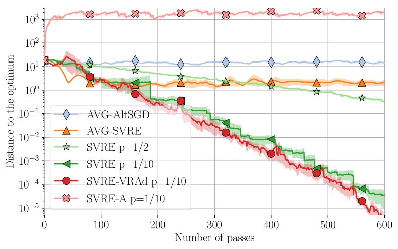
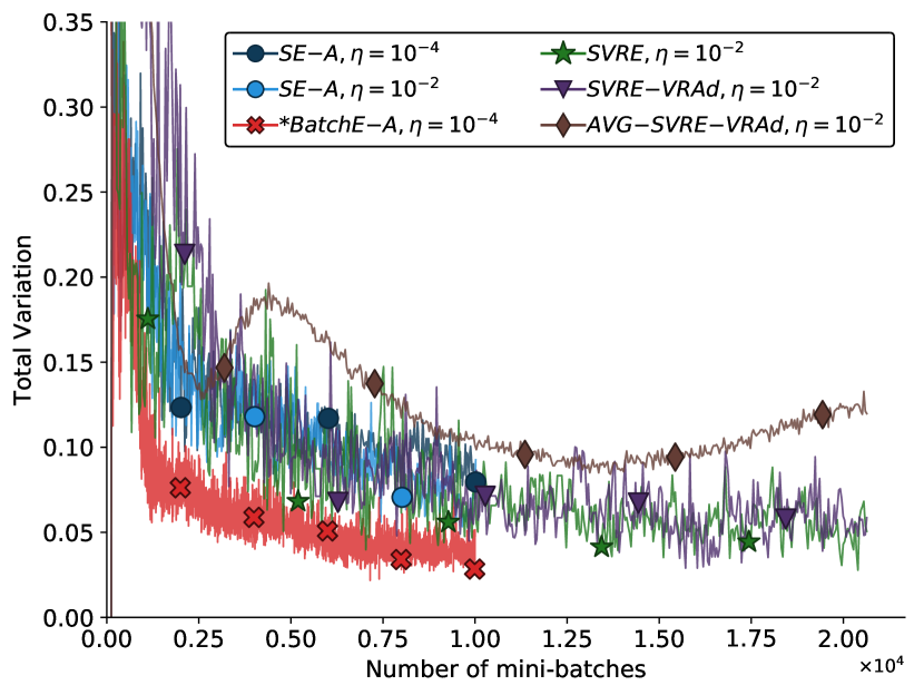
We compare variants of the following algorithms (with uniform sampling and average our results over 5 different seeds): (i) AltSGD: the standard method to train GANs–stochastic gradient with alternating updates of each player. (ii) SVRE: Alg. 1. The AVG prefix correspond to the uniform average of the iterates, . We observe in Fig. 4 that AVG-SVRE converges sublinearly (whereas AVG-AltSGD fails to converge).
This motivates a new variant of SVRE based on the idea that even if the averaged iterate converges, we do not compute the gradient at that point and thus we do not benefit from the fact that this iterate is closer to the optimums (see § A.1). Thus the idea is to occasionally restart the algorithm, i.e., consider the averaged iterate as the new starting point of our algorithm and compute the gradient at that point. Restart goes well with SVRE as we already occasionally stop the inner loop to recompute , at which point we decide (with a probability to be fixed) whether or not to restart the algorithm by taking the snapshot at point instead of . This variant of SVRE is described in Alg. 3 in § E and the variant combining VRAd in § D.1.
In Fig. 4 we observe that the only method that converges is SVRE and its variants. We do not provide convergence guarantees for Alg. 3 and leave its analysis for future work. However, it is interesting that, to our knowledge, this algorithm is the only stochastic algorithm (excluding batch extragradient as it is not stochastic) that converge for (24). Note that we tried all the algorithms presented in Fig. 3 from Gidel et al. (2019a) on this unconstrained problem and that all of them diverge.
4 GAN Experiments
In this section, we investigate the empirical performance of SVRE for GAN training. Note, however, that our theoretical analysis does not hold for games with non-convex objectives such as GANs.
Datasets. We used the following datasets: (i) MNIST(Lecun and Cortes, ), (ii) CIFAR-10(Krizhevsky, 2009, §3), (iii) SVHN(Netzer et al., 2011), and (iv) ImageNetILSVRC 2012 (Russakovsky et al., 2015), using , , , and resolution, respectively.
Metrics. We used the Inception score (IS, Salimans et al., 2016) and the Fréchet Inception distance (FID, Heusel et al., 2017) as performance metrics for image synthesis. To gain insights if SVRE indeed reduces the variance of the gradient estimates, we used the second moment estimate–SME (uncentered variance), computed with an exponentially moving average. See § F.1 for details.
DNN architectures. For experiments on MNIST, we used the DCGAN architectures (Radford et al., 2016), described in § F.2.1. For real-world datasets, we used two architectures (see § F.2 for details and § F.2.2 for motivation): (i) SAGAN (Zhang et al., 2018), and (ii) ResNet, replicating the setup of Miyato et al. (2018), described in detail in § F.2.3 and F.2.4, respectively. For clarity, we refer the former as shallow, and the latter as deep architectures.
Optimization methods.
We conduct experiments using the following optimization methods for GANs: (i) BatchE:full–batch extragradient, (ii) SG:stochastic gradient (alternating GAN), and (iii) SE:stochastic extragradient, and (iv) SVRE:stochastic variance reduced extragradient. These can be combined with adaptive learning rate methods such as Adam or with parameter averaging, hereafter denoted as –A and AVG–, respectively. In § D.1, we present a variant of Adam adapted to variance reduced algorithms, that is referred to as –VRAd. When using the SE–A baseline and deep architectures, the convergence rapidly fails at some point of training (cf. § G.3). This motivates experiments where we start from a stored checkpoint taken before the baseline diverged, and continue training with SVRE. We denote these experiments with WS–SVRE (warm-start SVRE).
4.1 Results
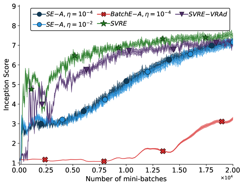
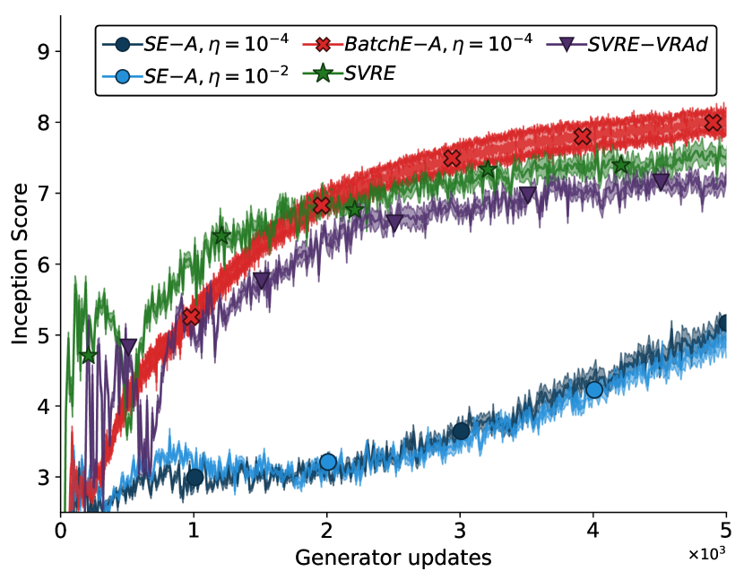
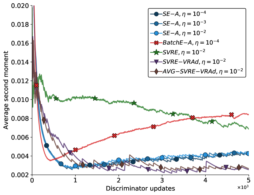
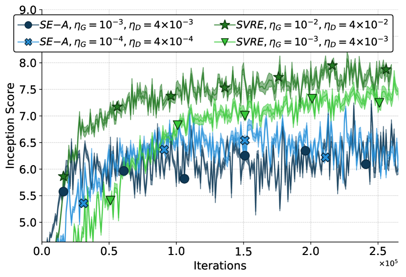
Comparison on MNIST. The MNIST common benchmark allowed for comparison with full-batch extragradient, as it is feasible to compute. Fig. 3 depicts the IS metric while using either a stochastic, full-batch or variance reduced version of extragradient (see details of SVRE-GAN in § D.2). We always combine the stochastic baseline (SE) with Adam, as proposed by Gidel et al. (2019a). In terms of number of parameter updates, SVRE performs similarly to BatchE–A (see Fig. 4(a), § G). Note that the latter requires significantly more computation: Fig. 3(a) depicts the IS metric using the number of mini-batch computations as x-axis (a surrogate for the wall-clock time, see below). We observe that, as SE–A has slower per-iteration convergence rate, SVRE converges faster on this dataset. At the end of training, all methods reach similar performances (IS is above , see Table 9, § G).
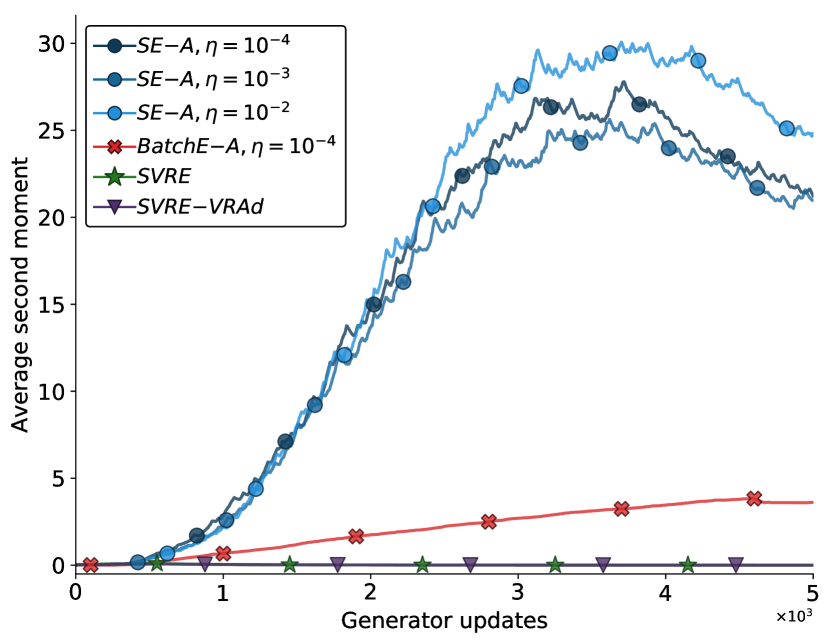
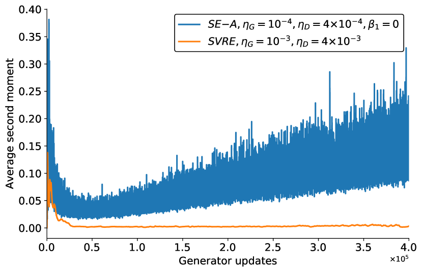
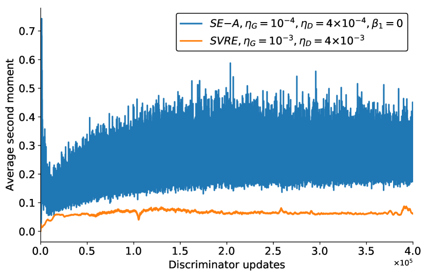
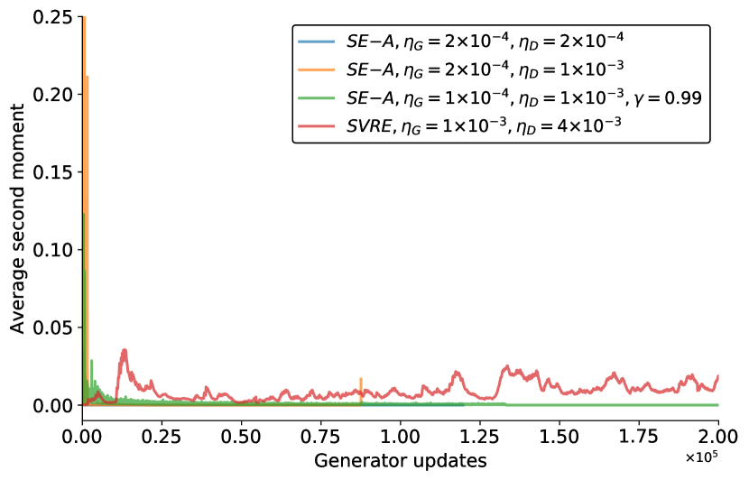
Computational cost. The relative cost of one pass over the dataset for SVRE versus vanilla SGD is a factor of : the full batch gradient is computed (on average) after one pass over the dataset, giving a slowdown of ; the factor takes into account the extra stochastic gradient computations for the variance reduction, as well as the extrapolation step overhead. However, as SVRE provides less noisy gradient, it may converge faster per iteration, compensating the extra per-update cost. Note that many computations can be done in parallel. In Fig. 3(a), the x-axis uses an implementation-independent surrogate for wall-clock time that counts the number of mini-batch gradient computations. Note that some training methods for GANs require multiple discriminator updates per generator update, and we observed that to stabilize our baseline when using the deep architectures it was required to use update ratio of (cf. § G.3), whereas for SVRE we used ratio of (Tab. 2 lists the results). Second moment estimate and Adam. Fig. 3(b) depicts the averaged second-moment estimate for parameters of the Generator, where we observe that SVRE effectively reduces it over the iterations. The reduction of these values may be the reason why Adam combined with SVRE performs poorly (as these values appear in the denominator, see § D.1). To our knowledge, SVRE is the first optimization method with a constant step size that has worked empirically for GANs on non-trivial datasets.
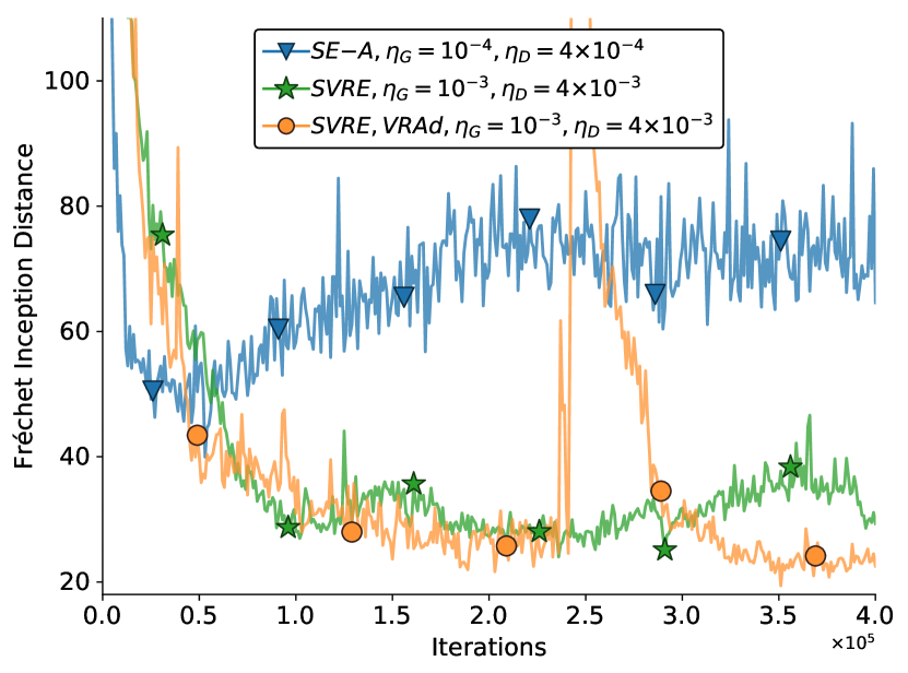
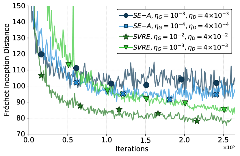
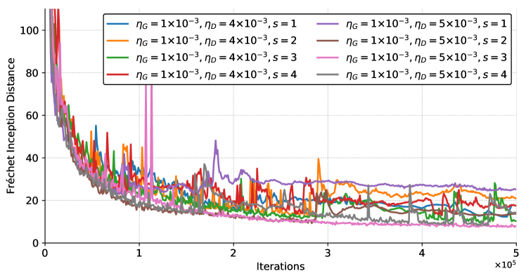
Comparison on real-world datasets. In Fig. 3(c), we compare SVRE with the SE–A baseline on SVHN, using shallow architectures. We observe that although SE–A in some experiments obtains better performances in the early iterations, SVRE allows for obtaining improved final performances. Tab. 2 summarizes the results on CIFAR-10 and SVHN with deep architectures. We observe that, with deeper architectures, SE–A is notably more unstable, as training collapsed in % of the experiments. To obtain satisfying results for SE–A, we used various techniques such as a schedule of the learning rate and different update ratios (see § G.3). On the other hand, SVRE did not collapse in any of the experiments but took longer time to converge compared to SE–A. Interestingly, although WS–SVRE starts from an iterate point after which the baseline diverges, it continues to improve the obtained FID score and does not diverge. See § G for additional experiments.
5 Related work
Surprisingly, there exist only a few works on variance reduction methods for monotone operators, namely from Palaniappan and Bach (2016) and Davis (2016). The latter requires a co-coercivity assumption on the operator and thus only convex optimization is considered. Our work provides a new way to use variance reduction for monotone operators, using the extragradient method (Korpelevich, 1976). Recently, Iusem et al. (2017) proposed an extragradient method with variance reduction for an infinite sum of operators. The authors use mini-batches of growing size in order to reduce the variance of their algorithm and to converge with a constant step-size. However, this approach is prohibitively expensive in our application. Moreover, Iusem et al. are not using the SAGA/SVRG style of updates exploiting the finite sum formulation, leading to sublinear convergence rate, while our method benefits from a linear convergence rate exploiting the finite sum assumption.
Daskalakis et al. (2018) proposed a method called Optimistic-Adam inspired by game theory. This method is closely related to extragradient, with slightly different update scheme. More recently, Gidel et al. (2019a) proposed to use extragradient to train GANs, introducing a method called ExtraAdam. This method outperformed Optimistic-Adam when trained on CIFAR-10. Our work is also an attempt to find principled ways to train GANs. Considering that the game aspect is better handled by the extragradient method, we focus on the optimization issues arising from the noise in the training procedure, a disregarded potential issue in GAN training.
In the context of deep learning, despite some very interesting theoretical results on non-convex minimization (Reddi et al., 2016; Allen-Zhu and Hazan, 2016), the effectiveness of variance reduced methods is still an open question, and a recent technical report by Defazio and Bottou (2018) provides negative empirical results on the variance reduction aspect. In addition, two recent large scale studies showed that increased batch size has: (i) only marginal impact on single objective training (Shallue et al., 2018) and (ii) a surprisingly large performance improvement on GAN training (Brock et al., 2019). In our work, we are able to show positive results for variance reduction in a real-world deep learning setting. This unexpected difference seems to confirm the remarkable discrepancy, that remains poorly understood, between multi-objective optimization and standard minimization.
6 Discussion
Motivated by a simple bilinear game optimization problem where stochasticity provably breaks the convergence of previous stochastic methods, we proposed the novel SVRE algorithm that combines SVRG with the extragradient method for optimizing games. On the theory side, SVRE improves upon the previous best results for strongly-convex games, whereas empirically, it is the only method that converges for our stochastic bilinear game counter-example.
We empirically observed that SVRE for GAN training obtained convergence speed similar to Batch-Extragradient on MNIST, while the latter is computationally infeasible for large datasets. For shallow architectures, SVRE matched or improved over baselines on all four datasets. Our experiments with deeper architectures show that SVRE is notably more stable with respect to hyperparameter choice. Moreover, while its stochastic counterpart diverged in all our experiments, SVRE did not. However, we observed that SVRE took more iterations to converge when using deeper architectures, though notably, we were using constant step-sizes, unlike the baselines which required Adam. As adaptive step-sizes often provide significant improvements, developing such an appropriate version for SVRE is a promising direction for future work. In the meantime, the stability of SVRE suggests a practical use case for GANs as warm-starting it just before the baseline diverges, and running it for further improvements, as demonstrated with the WS–SVRE method in our experiments.
Acknowledgements
This research was partially supported by the Canada CIFAR AI Chair Program, the Canada Excellence Research Chair in “Data Science for Realtime Decision-making”, by the NSERC Discovery Grant RGPIN-2017-06936, by the Hasler Foundation through the MEMUDE project, and by a Google Focused Research Award. Authors would like to thank Compute Canada for providing the GPUs used for this research. TC would like to thank Sebastian Stich and Martin Jaggi, and GG and TC would like to thank Hugo Berard for helpful discussions.
References
- Allen-Zhu and Hazan (2016) Z. Allen-Zhu and E. Hazan. Variance reduction for faster non-convex optimization. In ICML, 2016.
- Azizian et al. (2019) W. Azizian, I. Mitliagkas, S. Lacoste-Julien, and G. Gidel. A tight and unified analysis of extragradient for a whole spectrum of differentiable games. arXiv preprint arXiv:1906.05945, 2019.
- Bottou (2010) L. Bottou. Large-scale machine learning with stochastic gradient descent. In COMPSTAT, 2010.
- Boyd and Vandenberghe (2004) S. Boyd and L. Vandenberghe. Convex optimization. Cambridge university press, 2004.
- Brock et al. (2019) A. Brock, J. Donahue, and K. Simonyan. Large scale GAN training for high fidelity natural image synthesis. In ICLR, 2019.
- Daskalakis et al. (2018) C. Daskalakis, A. Ilyas, V. Syrgkanis, and H. Zeng. Training GANs with optimism. In ICLR, 2018.
- Davis (2016) D. Davis. Smart: The stochastic monotone aggregated root-finding algorithm. arXiv:1601.00698, 2016.
- Defazio and Bottou (2018) A. Defazio and L. Bottou. On the ineffectiveness of variance reduced optimization for deep learning. arXiv:1812.04529, 2018.
- Defazio et al. (2014) A. Defazio, F. Bach, and S. Lacoste-Julien. Saga: A fast incremental gradient method with support for non-strongly convex composite objectives. In NIPS, 2014.
- Facchinei and Pang (2003) F. Facchinei and J.-S. Pang. Finite-Dimensional Variational Inequalities and Complementarity Problems Vol I. Springer Series in Operations Research and Financial Engineering, Finite-Dimensional Variational Inequalities and Complementarity Problems. Springer-Verlag, 2003.
- Gidel et al. (2019a) G. Gidel, H. Berard, P. Vincent, and S. Lacoste-Julien. A variational inequality perspective on generative adversarial nets. In ICLR, 2019a.
- Gidel et al. (2019b) G. Gidel, R. A. Hemmat, M. Pezeshki, R. L. Priol, G. Huang, S. Lacoste-Julien, and I. Mitliagkas. Negative momentum for improved game dynamics. In AISTATS, 2019b.
- Glorot and Bengio (2010) X. Glorot and Y. Bengio. Understanding the difficulty of training deep feedforward neural networks. In AISTATS, 2010.
- Goodfellow et al. (2014) I. Goodfellow, J. Pouget-Abadie, M. Mirza, B. Xu, D. Warde-Farley, S. Ozair, A. Courville, and Y. Bengio. Generative adversarial nets. In NIPS, 2014.
- Harker and Pang (1990) P. T. Harker and J.-S. Pang. Finite-dimensional variational inequality and nonlinear complementarity problems: a survey of theory, algorithms and applications. Mathematical programming, 1990.
- He et al. (2015) K. He, X. Zhang, S. Ren, and J. Sun. Deep residual learning for image recognition. arXiv:1512.03385, 2015.
- Heusel et al. (2017) M. Heusel, H. Ramsauer, T. Unterthiner, B. Nessler, and S. Hochreiter. GANs trained by a two time-scale update rule converge to a local nash equilibrium. In NIPS, 2017.
- Hofmann et al. (2015) T. Hofmann, A. Lucchi, S. Lacoste-Julien, and B. McWilliams. Variance reduced stochastic gradient descent with neighbors. In NIPS, 2015.
- Ioffe and Szegedy (2015) S. Ioffe and C. Szegedy. Batch normalization: Accelerating deep network training by reducing internal covariate shift. In ICML, 2015.
- Iusem et al. (2017) A. Iusem, A. Jofré, R. I. Oliveira, and P. Thompson. Extragradient method with variance reduction for stochastic variational inequalities. SIAM Journal on Optimization, 2017.
- Johnson and Zhang (2013) R. Johnson and T. Zhang. Accelerating stochastic gradient descent using predictive variance reduction. In NIPS, 2013.
- Juditsky et al. (2011) A. Juditsky, A. Nemirovski, and C. Tauvel. Solving variational inequalities with stochastic mirror-prox algorithm. Stochastic Systems, 2011.
- Kingma and Ba (2015) D. P. Kingma and J. Ba. Adam: A method for stochastic optimization. In ICLR, 2015.
- Korpelevich (1976) G. Korpelevich. The extragradient method for finding saddle points and other problems. Matecon, 1976.
- Krizhevsky (2009) A. Krizhevsky. Learning Multiple Layers of Features from Tiny Images. Master’s thesis, 2009.
- Leblond et al. (2018) R. Leblond, F. Pederegosa, and S. Lacoste-Julien. Improved asynchronous parallel optimization analysis for stochastic incremental methods. JMLR, 19(81):1–68, 2018.
- (27) Y. Lecun and C. Cortes. The MNIST database of handwritten digits. URL http://yann.lecun.com/exdb/mnist/.
- Lim and Ye (2017) J. H. Lim and J. C. Ye. Geometric GAN. arXiv:1705.02894, 2017.
- Mescheder et al. (2017) L. Mescheder, S. Nowozin, and A. Geiger. The numerics of GANs. In NIPS, 2017.
- Miyato et al. (2018) T. Miyato, T. Kataoka, M. Koyama, and Y. Yoshida. Spectral normalization for generative adversarial networks. In ICLR, 2018.
- Netzer et al. (2011) Y. Netzer, T. Wang, A. Coates, A. Bissacco, B. Wu, and A. Y. Ng. Reading digits in natural images with unsupervised feature learning. 2011. URL http://ufldl.stanford.edu/housenumbers/.
- Palaniappan and Bach (2016) B. Palaniappan and F. Bach. Stochastic variance reduction methods for saddle-point problems. In NIPS, 2016.
- Radford et al. (2016) A. Radford, L. Metz, and S. Chintala. Unsupervised representation learning with deep convolutional generative adversarial networks. In ICLR, 2016.
- Reddi et al. (2016) S. J. Reddi, A. Hefny, S. Sra, B. Poczos, and A. Smola. Stochastic variance reduction for nonconvex optimization. In ICML, 2016.
- Robbins and Monro (1951) H. Robbins and S. Monro. A stochastic approximation method. The Annals of Mathematical Statistics, 1951.
- Russakovsky et al. (2015) O. Russakovsky, J. Deng, H. Su, J. Krause, S. Satheesh, S. Ma, Z. Huang, A. Karpathy, A. Khosla, M. Bernstein, A. C. Berg, and L. Fei-Fei. ImageNet Large Scale Visual Recognition Challenge. IJCV, 115(3):211–252, 2015.
- Salimans et al. (2016) T. Salimans, I. Goodfellow, W. Zaremba, V. Cheung, A. Radford, and X. Chen. Improved techniques for training GANs. In NIPS, 2016.
- Schaul et al. (2013) T. Schaul, S. Zhang, and Y. LeCun. No more pesky learning rates. In ICML, 2013.
- Schmidt et al. (2017) M. Schmidt, N. Le Roux, and F. Bach. Minimizing finite sums with the stochastic average gradient. Mathematical Programming, 2017.
- Shallue et al. (2018) C. J. Shallue, J. Lee, J. Antognini, J. Sohl-Dickstein, R. Frostig, and G. E. Dahl. Measuring the effects of data parallelism on neural network training. arXiv:1811.03600, 2018.
- Szegedy et al. (2015) C. Szegedy, V. Vanhoucke, S. Ioffe, J. Shlens, and Z. Wojna. Rethinking the inception architecture for computer vision. arXiv:1512.00567, 2015.
- Tseng (1995) P. Tseng. On linear convergence of iterative methods for the variational inequality problem. Journal of Computational and Applied Mathematics, 1995.
- Wilson et al. (2017) A. C. Wilson, R. Roelofs, M. Stern, N. Srebro, and B. Recht. The marginal value of adaptive gradient methods in machine learning. In NIPS, 2017.
- Xiao and Zhang (2014) L. Xiao and T. Zhang. A proximal stochastic gradient method with progressive variance reduction. SIAM Journal on Optimization, 24(4):2057–2075, 2014.
- Zhang et al. (2018) H. Zhang, I. Goodfellow, D. Metaxas, and A. Odena. Self-Attention Generative Adversarial Networks. arXiv:1805.08318, 2018.
Appendix A Noise in games
A.1 Why is convergence of the last iterate preferable?
In light of Theorem 1, the behavior of the iterates on the unconstrained version of (24) ():
| (12) |
where and are compact and convex sets, is the following: they will diverge until they reach the boundary of and and then they will start to turn around the Nash equilibrium of (12) lying on these boundaries. Using convexity properties, we can then show that the averaged iterates will converge to the Nash equilibrium of the problem. However, with an arbitrary large domain, this convergence rate may be arbitrary slow (since it depends on the diameter of the domain).
Moreover, this behavior might be even more problematic in a non-convex framework because even if by chance we initialize close to the Nash equilibrium, we would get away from it and we cannot rely on convexity to expect the average of the iterates to converge.
Consequently, we would like optimization algorithms generating iterates that stay close to the Nash equilibrium.
Appendix B Definitions and Lemmas
B.1 Smoothness and Monotonicity of the operator
Another important property used is the Lipschitzness of an operator.
Definition 4.
A mapping is said to be -Lipschitz if,
| (13) |
Definition 5.
A differentiable function is said to be -strongly convex if
| (14) |
Definition 6.
A function is said convex-concave if is convex for all and is concave for all . An is said to be -strongly convex concave if is convex concave.
Definition 7.
For , an operator is said to be -strongly monotone if ,
where we noted .
Definition 8.
An operator is said to be -cocoercive, if for all we have
| (15) |
Proposition 1 (Folklore).
A -Lipschitz and -strongly monotone operator is -cocoercive
Proof.
By applying lipschitzness and strong monotonicity,
| (16) |
∎
Proposition 2.
If , where and are -strongly convex and smooth, then is a sufficient condition for to be -cocoercive with
Proof.
We rewrite as the sum of the gradient of convex Lipschitz function and a -Lipschitz and -strongly monotone operator :
| (17) |
Then
| (18) | ||||
| (19) | ||||
| (20) | ||||
| (21) | ||||
| (22) | ||||
| (23) |
where for the second inequality we used that a -Lipschitz convex function is -cocoercive and Proposition 2. ∎
Appendix C Proof of Theorems
C.1 Proof of Theorem 1
Proof.
We consider the following stochastic optimization problem,
| (24) |
where if and otherwise. Note that for . Let us consider the extragradient method where to compute an unbiased estimator of the gradients at we sample and use as estimator of the vector flow.
In this proof we note, and the vector such that if and otherwise. Note that and that .
Thus the extragradient update rule can be noted as
| (25) |
where is the mini-batch sampled (without replacement) for the update and the mini-batch sampled (without replacement) for the extrapolation.
We can thus notice that, when , we have
| (26) |
and otherwise,
| (27) |
The intuition is that, on one hand, when (which happens with high probability when , e.g., when , ), the algorithm performs an update that get away from the Nash equilibrium when :
| (28) |
where and . On the other hand, The updates that provide improvement only happen when is large (which happen with low probability, e.g., when , ):
| (29) |
Conditioning on and , we get that
| (30) |
Leading to,
| (31) |
Plugging these expectations in (29), we get that,
| (32) |
Consequently for we get,
| (33) |
To sum-up, if is not large enough (more precisely if ), we have the geometric divergence of the quantity for any . ∎
C.2 Proof of Theorem 2
Setting of the Proof.
We will prove a slightly more general result than Theorem 2. We will work in the context of monotone operator. Let us consider the general extrapolation update rule,
| (34) |
where depends on and depends on . For instance, can either be , or the SVRG estimate defined in (46).
Let us first state a lemma standard in convex analysis (see for instance (Boyd and Vandenberghe, 2004)),
Lemma 1.
Let and then for all we have,
| (35) |
Proof of Lemma 1.
We start by simply developing,
Then since is the projection onto the convex set of we have that , leading to the result of the Lemma. ∎
Lemma 2.
If is -strongly monotone for any we have,
| (36) |
where we noted .
Proof.
By -strong monotonicity,
| (37) |
and then we use the inequality to get the result claimed. ∎
Using this update rule we can thus deduce the following lemma, the derivation of this lemma is very similar from the derivation of Harker and Pang (1990, Lemma 12.1.10).
Lemma 3.
Considering the update rule (34), we have for any and any ,
| (38) |
Proof.
Note that if we would have set and any estimate of the gradient at we recover the standard lemma for gradient method.
Let us consider unbiased estimates of the gradient,
| (46) |
where , the index are (potentially) non-uniformly sampled from with replacement according to and . Hence we have that , where the expectation is taken with respect to the index sampled from .
We will consider a class of algorithm called uniform memorization algorithms first introduced by (Hofmann et al., 2015). This class of algorithms describes a large subset of variance reduced algorithms taking advantage of the finite sum formulation such as SAGA (Defazio et al., 2014), SVRG (Johnson and Zhang, 2013) or -SAGA and -SAGA (Hofmann et al., 2015). In this work, we will use a slightly more general definition of such algorithm in order to be able to handle extrapolation steps:
Definition 9 (Extension of (Hofmann et al., 2015)).
In the case of SVRG, either or (when we update the snapshot).
We have the following lemmas,
Lemma 4.
For any , if we consider a -memorization algorithm we have
Proof.
We use an extended version of Young’s inequality: ,
where we used that . We combine Young’s inequality with the definition of -memorization algorithm: and to get (we omit the subscript for and and we note ),
Notice that since and are independently sampled from the same distribution we have
| (48) |
Note that we have (using that and ),
| (49) |
By assuming that each is -Lipschitz we get,
| (50) | ||||
| (51) | ||||
| (52) |
where . Note that and do not depend on (which is the index sampled for the update step), that is not the case for (the index for the extrapolation step) since is the result of the extrapolation. ∎
This lemma make appear the quantity that we need to bound. In order to do that we prove the following lemma,
Lemma 5.
Let be updated according to the rules of a -uniform memorization algorithm (Def. 9). Let us note . For any ,
| (53) |
Proof.
We will use the definition of -uniform memorization algorithms (saying that is updated at time with probability ). We call this event " updated",
∎
Using all these lemmas we can prove our theorem.
Theorem’ 2.
Under Assumption 1, after iterations, the iterate computed by a -memorization algorithm with step-sizes verifies:
| (54) |
Proof.
In this proof we will consider a constant step-size . For simplicity of notations we will consider the notation,
We start by recalling Lemma 3,
| (55) |
We can then take the expectation and plug-in the expression of from Lemma 4,
Let us define , where . We can combine (55) with Lemma 5 multiplied by a constant that we will set later to get
Since and are independently drawn from the same distribution, we have, and thus,
where for the second inequality we used Young’s inequality and the Lipchitzness of and for the last one we used the co-coercivity of :
| (56) |
Thus using , we get
where . Now we can set to get
By using the strong convexity of and Young’s inequality we have that
| (57) |
Finally with (note that we always have because ) we get
We finally use the projection-type error bound the same way as (Azizian et al., 2019) to get,
Thus we have that,
where . We can thus conclude the proof using the strong convexity of ,
Appendix D Details on the SVRE–GAN Algorithm
D.1 Practical Aspect
Noise dataset.
Variance reduction is usually performed on finite sum dataset. However, the noise dataset in GANs (sampling from the noise variable for the generator ) is in practice considered as an infinite dataset. We considered several ways to cope with this:
-
•
Infinitely taking new samples from a predefined latent distribution . In this case, from a theoretical point of view, in terms of using finite sum formulation, there is no convergence guarantee for SVRE even in the strongly convex case. Moreover, the estimators (65) and (66) are biased estimator of the gradient (as and do not estimate the full expectation but a finite sum).
-
•
Sampling a different noise dataset at each epoch, i.e. considering a different finite sum at each epoch. In that case, we are performing a variance reduction of this finite sum over the epoch.
-
•
Fix a finite sum noise dataset for the entire training.
In practice, we did not notice any notable difference between the three alternatives.
Adaptive methods.
Particular choices such as the optimization method (e.g. Adam (Kingma and Ba, 2015)), learning rates, and normalization, have been established in practice as almost prerequisite for convergence555For instance, Daskalakis et al. (2018); Gidel et al. (2019a) plugged Adam into their principled method to get better results., in contrast to supervised classification problems where they have been shown to only provide a marginal value (Wilson et al., 2017). To our knowledge, SVRE is the only method that works with a constant step size for GANs on non-trivial datasets. This combined with the fact that recent works empirically tune the first moment controlling hyperparameter to (, see below) and the variance reduction (VR) one (, see below) to a non-zero value, sheds light on the reason behind the success of Adam on GANs.
However, combining SVRE with adaptive step size scheme on GANs remains an open problem. We first briefly describe the update rule of Adam, and then we propose a new adaptation of it that is more suitable for VR methods, which we refer to as variance reduced Adam (VRAd).
Adam.
Adam stores an exponentially decaying average of both past gradients and squared gradients , for each parameter of the model:
| (58) | |||
| (59) |
where , , , and denotes the iteration. and are respectively the estimates of the first and the second moments of the stochastic gradient. To compensate the bias toward due to initialization, Kingma and Ba (2015) propose to use bias-corrected estimates of these first two moments:
| (60) | |||
| (61) |
The Adam update rule can be described as:
| (62) |
Adam can be understood as an approximate gradient method with a diagonal step size of . Since VR methods aim to provide a vanishing , they lead to a too large step-size of . This could indicate that the update rule of Adam may not be a well-suited method to combine with VR methods.
VRAd.
This motivates the introduction of a new Adam-inspired variant of adaptive step sizes that maintain a reasonable size even when vanishes,
| (VRAd) |
This adaptive variant of Adam is motivated by the step size derived by Schaul et al. (2013). (VRAd) is simply the square-root of in order to stick with Adam’s scaling of .
D.2 SVRE-GAN
In order to cope with the issues introduced by the stochastic game formulation of the GAN models, we proposed the SVRE algorithm Alg. 1 which combines SVRG and extragradient method. We refer to the method of applying SVRE to train GANs as the SVRE-GAN method, and we describe it in detail in Alg. 2 (generalizing it with mini-batching, but using uniform probabilities). Assuming that we have and , respectively two mini-batches of size of the true dataset and the noise dataset, we compute and the respective mini-batches gradient of the discriminator and the generator:
| (63) | |||
| (64) |
where and are respectively the example of the noise dataset and the of the true dataset. Note that and are lists and thus that we allow repetitions in the summations over and . The variance reduced gradient of the SVRG method are thus given by:
| (65) | ||||
| (66) |
where and are the snapshots and and their respective gradients.
Alg. 2 summarizes the SVRG optimization extended to GAN. To obtain that vanishes, when updating and where the expectation is over samples of and respectively, we use the snapshot networks and for the second term in lines and . Moreover, the noise dataset , where , is fixed. Empirically we observe that directly sampling from (contrary to fixing the noise dataset and re-sampling it with frequency ) does not impact the performance, as is usually high.
Note that the double sum in Line can be written as two sums because of the separability of the expectations in typical GAN objectives. Thus the time complexity for calculating is still and not which would be prohibitively expensive.
Appendix E Restarted SVRE
Appendix F Details on the implementation
For our experiments, we used the PyTorch666https://pytorch.org/ deep learning framework, whereas for computing the FID and IS metrics, we used the provided implementations in Tensorflow777https://www.tensorflow.org/.
F.1 Metrics
We provide more details about the metrics enumerated in § 4. Both FID and IS use: (i) the Inception v3 network (Szegedy et al., 2015) that has been trained on the ImageNet dataset consisting of million RGB images of classes, . (ii) a sample of generated images , where usually .
F.1.1 Inception Score
Given an image , IS uses the softmax output of the Inception network which represents the probability that is of class , i.e., . It then computes the marginal class distribution . IS measures the Kullback–Leibler divergence between the predicted conditional label distribution and the marginal class distribution . More precisely, it is computed as follows:
| (67) |
It aims at estimating (i) if the samples look realistic i.e., should have low entropy, and (ii) if the samples are diverse (from different ImageNet classes) i.e., should have high entropy. As these are combined using the Kullback–Leibler divergence, the higher the score is, the better the performance. Note that the range of IS scores at convergence varies across datasets, as the Inception network is pretrained on the ImageNet classes. For example, we obtain low IS values on the SVHN dataset as a large fraction of classes are numbers, which typically do not appear in the ImageNet dataset. Since MNIST has greyscale images, we used a classifier trained on this dataset and used . For the rest of the datasets, we used the original implementation888https://github.com/openai/improved-gan/ of IS in TensorFlow, and .
F.1.2 Fréchet Inception Distance
Contrary to IS, FID aims at comparing the synthetic samples with those of the training dataset in a feature space. The samples are embedded using the first several layers of the Inception network. Assuming and are multivariate normal distributions, it then estimates the means and and covariances and , respectively for and in that feature space. Finally, FID is computed as:
| (68) |
where denotes the Fréchet Distance. Note that as this metric is a distance, the lower it is, the better the performance. We used the original implementation of FID999https://github.com/bioinf-jku/TTUR in Tensorflow, along with the provided statistics of the datasets.
F.1.3 Second Moment Estimate
To evaluate SVRE effectively, we used the second moment estimate (SME, uncentered variance, see § D.1) of the gradient estimate throughout the iterations per parameter, computed as: , where denotes the gradient estimate for the parameter and iteration , and . For SVRE, is and (see Eq. 65 and 66) for and , respectively. We initialize and we use bias-corrected estimates: . As the second moment estimate is computed per each parameter of the model, we depict the average of these values for the parameters of and separately.
In this work, as we aim at assessing if SVRE effectively reduces the variance of the gradient updates, we use SME in our analysis as it is computationally inexpensive and fast to compute.
F.1.4 Entropy & Total Variation on MNIST
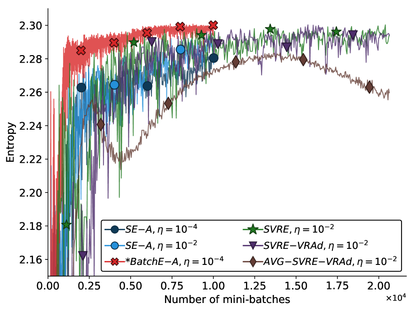
For the experiments on MNIST illustrated in Fig. 4(a) & 3(b) in § 4, we plot in § G the entropy (E) of the generated samples’ class distribution, as well as the total variation (TV) between the class distribution of the generated samples and a uniform one (both computed using a pretrained network that classifies its classes).
F.2 Architectures & Hyperparameters
Description of the architectures.
We describe the models we used in the empirical evaluation of SVRE by listing the layers they consist of, as adopted in GAN works, e.g. (Miyato et al., 2018). With “conv.” we denote a convolutional layer and “transposed conv” a transposed convolution layer (Radford et al., 2016). The models use Batch Normalization (Ioffe and Szegedy, 2015) and Spectral Normalization layers (Miyato et al., 2018).
F.2.1 Architectures for experiments on MNIST
For experiments on the MNIST dataset, we used the DCGAN architectures (Radford et al., 2016), listed in Table 3, and the parameters of the models are initialized using PyTorch default initialization. We used mini-batch sizes of samples, whereas for full dataset passes we used mini-batches of samples as this reduces the wall-clock time for its computation. For experiments on this dataset, we used the non saturating GAN loss as proposed (Goodfellow et al., 2014):
| (69) | |||
| (70) |
where and denote the data and the latent distributions (the latter to be predefined).
For both the baseline and the SVRE variants we tried the following step sizes . We observe that SVRE can be used with larger step sizes. In Table 9, we used and for SE–A and SVRE(–VRAd), respectively.
| Generator |
|---|
| Input: |
| \hdashlinetransposed conv. (ker: , ; stride: ) |
| Batch Normalization |
| ReLU |
| transposed conv. (ker: , , stride: ) |
| Batch Normalization |
| ReLU |
| transposed conv. (ker: , , stride: ) |
| Batch Normalization |
| ReLU |
| transposed conv. (ker: , , stride: , pad: 1) |
| Discriminator |
|---|
| Input: |
| \hdashlineconv. (ker: , ; stride: ; pad:1) |
| LeakyReLU (negative slope: ) |
| conv. (ker: , ; stride: ; pad:1) |
| Batch Normalization |
| LeakyReLU (negative slope: ) |
| conv. (ker: , ; stride: ; pad:1) |
| Batch Normalization |
| LeakyReLU (negative slope: ) |
| conv. (ker: , ; stride: ) |
F.2.2 Choice of architectures on real-world datasets
We replicate the experimental setup described for CIFAR-10 and SVHN in (Miyato et al., 2018), described also below in § F.2.4. We observe that this experimental setup is highly sensitive to the choice of the hyperparameters (see our results in § G.3), making it more difficult to compare the optimization methods for a fixed hyperparameter choice. In particular, apart from the different combinations of learning rates for and , for the baseline this also included experimenting with: (see (58)), a multiplicative factor of exponential learning rate decay scheduling , as well as different ratio of updating and per iteration. These observations, combined with that we had limited computational resources, motivated us to use shallower architectures, which we describe below in § F.2.3, and which use an inductive bias of so-called Self–Attention layers (Zhang et al., 2018). As a reference, our SAGAN and ResNet architectures for CIFAR-10 have approximately and layers, respectively–in total for G and D, including the non linearity and the normalization layers. For clarity, although the deeper and the shallower architectures differ as they are based on ResNet and SAGAN, we refer these as deep (see § F.2.3) and shallow (see § F.2.4), respectively.
F.2.3 Shallower SAGAN architectures
We used the SAGAN architectures (Zhang et al., 2018), as the techniques of self-attention introduced in SAGAN were used to obtain the state-of-art GAN results on ImageNet (Brock et al., 2019). In summary, these architectures: (i) allow for attention-driven, long-range dependency modeling, (ii) use spectral normalization (Miyato et al., 2018) on both and (efficiently computed with the power iteration method); and (iii) use different learning rates for and , as advocated in (Heusel et al., 2017). The foremost is obtained by combining weights, or alternatively attention vectors, with the convolutions across layers, so as to allow modeling textures that are consistent globally–for the generator, or enforcing geometric constraints on the global image structure–for the discriminator.
We used the architectures listed in Table 5 for CIFAR-10 and SVHN datasets, and the architectures described in Table 6 for the experiments on ImageNet. The models’ parameters are initialized using the default initialization of PyTorch.
For experiments with SAGAN, we used the hinge version of the adversarial non-saturating loss (Lim and Ye, 2017; Zhang et al., 2018):
| (71) | |||
| (72) |
where consistent with the notation above, and denote the data and the latent distributions.
| Self–Attention Block ( – input depth) | ||
|---|---|---|
| Input: | ||
| \hdashline i: conv. (ker: , ) | ii: conv. (ker: , ) | iii: conv. (ker: , ) |
| iv: softmax( (i) (ii) ) | ||
| \hdashline Output: | ||
| Generator |
| Input: |
| transposed conv. (ker: , ; stride: ) |
| Spectral Normalization |
| Batch Normalization |
| ReLU |
| \hdashlinetransposed conv. (ker: , , stride: , pad: ) |
| Spectral Normalization |
| Batch Normalization |
| ReLU |
| \hdashlineSelf–Attention Block () |
| \hdashlinetransposed conv. (ker: , , stride: , pad: ) |
| Spectral Normalization |
| Batch Normalization |
| ReLU |
| \hdashlineSelf–Attention Block () |
| \hdashlinetransposed conv. (ker: , , stride: , pad: ) |
| Discriminator |
| Input: |
| conv. (ker: , ; stride: ; pad: ) |
| Spectral Normalization |
| LeakyReLU (negative slope: ) |
| \hdashlineconv. (ker: , ; stride: ; pad: ) |
| Spectral Normalization |
| LeakyReLU (negative slope: ) |
| \hdashlineconv. (ker: , ; stride: ; pad: ) |
| Spectral Normalization |
| LeakyReLU (negative slope: ) |
| \hdashlineSelf–Attention Block () |
| \hdashlineconv. (ker: , ; stride: ) |
| Generator |
| Input: |
| transposed conv. (ker: , ; stride: ) |
| Spectral Normalization |
| Batch Normalization |
| ReLU |
| \hdashlinetransposed conv. (ker: , , stride: , pad: ) |
| Spectral Normalization |
| Batch Normalization |
| ReLU |
| \hdashlinetransposed conv. (ker: , , stride: , pad: ) |
| Spectral Normalization |
| Batch Normalization |
| ReLU |
| \hdashlineSelf–Attention Block () |
| \hdashlinetransposed conv. (ker: , , stride: , pad: ) |
| Spectral Normalization |
| Batch Normalization |
| ReLU |
| \hdashlineSelf–Attention Block () |
| \hdashlinetransposed conv. (ker: , , stride: , pad: ) |
| Discriminator |
| Input: |
| conv. (ker: , ; stride: ; pad: ) |
| Spectral Normalization |
| LeakyReLU (negative slope: ) |
| \hdashlineconv. (ker: , ; stride: ; pad: ) |
| Spectral Normalization |
| LeakyReLU (negative slope: ) |
| \hdashlineconv. (ker: , ; stride: ; pad: ) |
| Spectral Normalization |
| LeakyReLU (negative slope: ) |
| \hdashlineSelf–Attention Block () |
| \hdashlineconv. (ker: , ; stride: ; pad: ) |
| Spectral Normalization |
| LeakyReLU (negative slope: ) |
| \hdashlineSelf–Attention Block () |
| \hdashlineconv. (ker: , ; stride: ) |
For the SE–A baseline we obtained best performances when and , for G and D, respectively. Similarly as noted for MNIST, using SVRE allows for using larger order of the step size on the rest of the datasets, whereas SE–A with increased step size ( and failed to converge. In Table 2, , , and , for SVRE and SVRE–VRAd, respectively. We did not use momentum for the vanilla SVRE experiments.
F.2.4 Deeper ResNet architectures
We experimented with ResNet (He et al., 2015) architectures on CIFAR-10 and SVHN, using the architectures listed in Table 8, that replicate the setup described in (Miyato et al., 2018) on CIFAR-10. For experiments with ResNet, we used the hinge version of the adversarial non-saturating loss, Eq. 71 and 72. For this architectures, we refer the reader to § G.3 for details on the hyperparameters, where we list the hyperparameters along with the obtained results.
| G–ResBlock |
|---|
| Bypass: |
| Upsample() |
| \hdashline Feedforward: |
| Batch Normalization |
| ReLU |
| Upsample() |
| conv. (ker: , ; stride: ; pad: ) |
| Batch Normalization |
| ReLU |
| conv. (ker: , ; stride: ; pad: ) |
| D–ResBlock (–th block) |
|---|
| Bypass: |
| AvgPool (ker: ), if |
| conv. (ker: , ; stride: ) |
| Spectral Normalization |
| AvgPool (ker:, stride:), if |
| \hdashline Feedforward: |
| ReLU , if |
| conv. (ker: , ; stride: ; pad: ) |
| Spectral Normalization |
| ReLU |
| conv. (ker: , ; stride: ; pad: ) |
| Spectral Normalization |
| AvgPool (ker: ) |
| Generator | Discriminator |
|---|---|
| Input: | Input: |
| \hdashlineLinear() | D–ResBlock |
| G–ResBlock | D–ResBlock |
| G–ResBlock | D–ResBlock |
| G–ResBlock | D–ResBlock |
| Batch Normalization | ReLU |
| ReLU | AvgPool (ker: ) |
| conv. (ker: , ; stride: ; pad:1) | Linear() |
| Spectral Normalization |
Appendix G Additional Experiments
G.1 Results on MNIST
| IS | FID | ||||||
|---|---|---|---|---|---|---|---|
| SE–A | SVRE | SVRE–VRAd | SE–A | SVRE | SVRE–VRAd | ||
| MNIST | |||||||
| CIFAR-10 | |||||||
| SVHN | |||||||
| ImageNet | |||||||
The results in Table 2 on MNIST are obtained using runs with different seeds, and the shown performances are the averaged values. Each experiment was run for iterations. The corresponding scores with the standard deviations are as follows: (i) IS: , , ; (ii) FID: , , ; for SE–A, SVRE, and SVRE–VRAd, respectively. On this dataset, we obtain similar final performances if run for many iterations, however SVRE converges faster (see Fig. 3). Fig. 5 illustrates additional metrics of the experiments shown in Fig. 3.
G.2 Results with shallow architectures
Fig. 6 depicts the results on ImageNet using the shallow architectures described in Table 6, § F.2.3. Table 9 summarizes the results obtained on SVHN, CIFAR-10 and ImageNet with these architectures. Fig. 7 depicts the SME metric (see § F.1.3) for the the SE–A baseline and SVRE shown in Fig. 3(c), on SVHN.
G.3 Results with deeper architectures
We observe that GAN training is more challenging when using deeper architectures and some empirical observations differ in the two settings. For example, our stochastic baseline is drastically more unstable and often does not start to converge, whereas SVRE is notably stable, but slower compared to when using shallower architectures. In this section, all our discussions focus on deep architectures (see § F.2.4).
Stability: convergence of the GAN training.
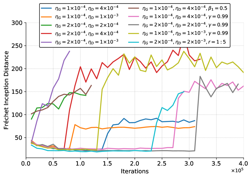
For our stochastic baselines, irrespective whether we use the extragradient or gradient method, we observe that the convergence is notably more unstable (see Fig. 8) when using the deep architectures described in § F.2.4. More precisely, either the training fails to converge or it diverges at later iterations. When updating G and D equal number of times i.e. using update ratio, using SE–A on CIFAR-10 we obtained best FID score of using , , while experimenting with several combinations of . Using exponential learning rate decay with a multiplicative factor of , improved the best FID score to , obtained for the experiment with , . Finally, using update ratio, with , provided best FID of for the baseline. Figures 7(a) and 7(b) depict the hyper-parameter sensitivity of SE–A and SG–A, respectively. The latter denotes the alternating GAN training with Adam, that is most commonly used for GAN training.
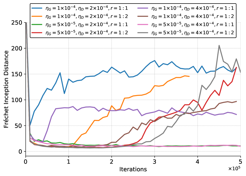
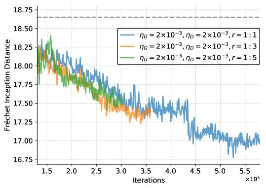
We observe that SVRE is more stable in terms of hyperparameter selection, as it always starts to converge and does not diverge at later iterations. Relative to experiments with shallower architectures, we observe that with deeper architectures SVRE takes longer to converge than its baseline for this architecture. With constant step size of , we obtain FID score of on CIFAR-10. Note that this result outperforms the baseline when using no additional tricks (which themselves require additional hyperparameter tuning). Fig. 9 depicts the FID scores obtained when training with SVRE on the SVHN dataset, for two different hyperparameter settings, using four different seeds for each. From this set of experiments, we observe that contrary to the baseline that either did not converge or diverged in all our experiments, SVRE always converges. However, we observe different performances for different seeds. This suggests that more exhaustive empirical hyperparameter search that aims to find an empirical setup that works best for SVRE or further combining SVRE with adaptive step size techniques are both promising research directions (see our discussion below). Fig. 10 depicts our WS–SVRE experiment, where we start from a stored checkpoint for which we obtained best FID score for the SE–A baseline, and we continue the training with SVRE. It is interesting that besides that the baseline diverged after the stored checkpoint, SVRE further reduced the FID score. Moreover, we observe that using different update ratios does not impact much the performance, what on the other hand was necessary to make the baseline algorithm converge.
Second moment estimate (SME).
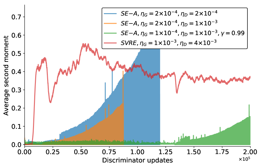
Fig. 11 depicts the second moment estimate (see § F.1.3) for the experiments with deep architectures. We observe that: (i) the estimated SME quantity is more bounded and changes more smoothly for SVRE (as we do not observe large oscillations of it as it is the case for SE–A); as well as that (ii) divergence of the SE–A baseline correlates with large oscillations of SME, in this case, observed for the Discriminator. Regarding the latter, there exist larger in magnitude oscillations of SME (note that the exponential moving average hyperparameter for computing SME is , see § F.1.3).
Conclusion & future directions.
In summary, we observe the following most important advantages of SVRE when using deep architectures: (i) consistency of convergence, and improved stability; as well as (ii) reduced number of hyperparameters. Apart from the practical benefit for applications, the former could allow for a more fair comparison of GAN variants. The latter refers to the fact that SVRE omits the tuning of the sensitive (for the stochastic baseline) hyperparameter (see (58)), as well as and –as training converges for SVRE without using different update ratio and step size schedule, respectively. It is important to note that the stochastic baseline does not converge when using constant step size (i.e. when SGD is used instead of Adam). In our experiments we compared SVRE that uses constant step size, with Adam, making the comparison unfair toward SVRE. Hence, our results indicate that SVRE can be further combined with adaptive step size schemes, so as to obtain both stable GAN performances and fast convergence when using these architectures. Nonetheless, the fact that the baseline either does not start to converge or it diverges later makes SVRE and WS–SVRE a promising approach for practitioners using these deep architectures, whereas, for shallower ones, SVRE speeds up the convergence and often provides better final performances.