Particle Energy Diffusion in Linear Magnetohydrodynamic Waves

Abstract

In high-energy astronomical phenomena, the stochastic particle acceleration by turbulences is one of the promising processes to generate non-thermal particles. In this paper, we investigate the energy-diffusion efficiency of relativistic particles in a temporally evolving wave ensemble that consists of a single mode (Alfvén, fast or slow) of linear magnetohydrodynamic waves. In addition to the gyroresonance with waves, the transit-time damping (TTD) also contributes to the energy-diffusion for fast and slow-mode waves. While the resonance condition with the TTD has been considered to be fulfilled by a very small fraction of particles, our simulations show that a significant fraction of particles are in the TTD resonance owing to the resonance broadening by the mirror force, which non-resonantly diffuses the pitch angle of particles. When the cutoff scale in the turbulence spectrum is smaller than the Larmor radius of a particle, the gyroresonance is the main acceleration mechanism for all the three wave modes. For the fast-mode, the coexistence of the gyroresonance and TTD resonance leads to anomalous energy-diffusion. For a particle with its Larmor radius smaller than the cutoff scale, the gyroresonance is negligible, and the TTD becomes the dominant mechanism to diffuse its energy. The energy-diffusion by the TTD-only resonance with fast-mode waves agrees with the hard-sphere-like acceleration suggested in some high-energy astronomical phenomena.

1. Introduction

The first-order Fermi acceleration at shock waves is the standard model to produce non-thermal particles in high-energy astrophysical objects. However, several objects show a very hard photon spectrum, which is hardly explained by the standard shock acceleration theory. While the magnetic reconnection as an alternative model has been discussed (e.g. Giannios, 2008; Uzdensky et al., 2011; Sironi & Spitkovsky, 2014; Sironi et al., 2015), the spectral-fitting models frequently suggest low magnetization in emission regions (e.g., Atoyan & Aharonian, 1996; Ackermann et al., 2016). Another possible model is the stochastic particle acceleration (SA) in turbulence (e.g., Achternerg, 1979; Ptuskin, 1988; Park & Petrosian, 1995; Schlickeiser & Miller, 1998; Becker et al., 2006; Cho & Lazarian, 2006; Stawartz & Petrosian, 2008). The SA model has been adopted for blazars (Böttcher, 1999; Schlickeiser & Dermer, 2000; Lefa et al., 2011; Asano et al., 2014; Asano & Hayashida, 2015; Kakuwa et al., 2015; Asano & Hayashida, 2018), gamma-ray bursts (Bykov & Mészáros, 1996; Asano & Terasawa, 2009, 2015; Murase et al., 2012; Asano & Mészáros, 2016; Xu & Zhang, 2017), pulsar wind nebula (Tanaka & Asano, 2017), supernova remnants (Liu et al., 2008; Fan et al., 2010), Fermi bubbles (Mertsch & Sarkar, 2011; Sasaki et al., 2015), radio galaxies (O’sullivan et al., 2009), and low-luminosity active galactic nuclei (AGNs) (Kimura et al., 2014, 2015).

Mechanisms of the SA in magnetohydrodynamic (MHD) turbulence have not yet been fully understood. One ambiguous point is in the wave-particle interactions. In the classical SA theory (see Blandford & Eichler, 1987, for a review), the gyroresonance with the Alfvén waves is considered as the main mechanism for the diffusion in the momentum space. Non-resonant acceleration caused by the adiabatic compression of the large-scale waves is studied by Ptuskin (1988) and Cho & Lazarian (2006). In high-energy astrophysical objects compressional waves (fast- and slow-mode waves) can also play a role in the particle acceleration process (Cho & Lazarian, 2003). For compressional waves, the transit-time damping (TTD, Berger et al., 1958) can contribute to accelerating particles as well. However, the fraction of particles in the TTD resonance has been considered very small.

The wave spectrum in turbulence, which affects the SA process, is different in each astronomical object. One of the most broadly accepted models is the Kolmogorov spectrum (Kolmogorov, 1941, hereafter K41), $E(k)\propto k^{-5/3}$, where $k$ is the wavenumber, and $\int E(k)dk$ is the kinetic energy of turbulence. In the K41 model, the system is isotropic and quasi-steady, and the cascade process is regulated by only the energy input rate at a large scale. However, the magnetic field can be a crucial factor in understanding the MHD turbulence, as the magnetic energy density is frequently comparable to the kinetic energy of turbulence.

Iroshnikov (1963) and Kraichnan (1965) (hereafter IK) included the effect of the magnetic field into their picture of isotropic turbulence. In the IK turbulence, the Alfvén velocity is a parameter that characterizes the system, and the energy distribution is expressed as $E(k)\propto k^{-3/2}$. For fast-mode waves, the IK turbulence is a reasonable approximation for several simulations (e.g. Cho et al., 2002). Kowal & Lazarian (2010) have shown an index $-2$ in simulations of fast-mode turbulence. The spectral index of fast-mode turbulence may depend on the simulation setup. The actual index in astronomical fast-mode turbulences is highly uncertain, while the anisotropic turbulence so-called Goldreich–Sridhar model (GS; Goldreich & Sridhar, 1995) is established for the slow and Alfvénic turbulence (see also Goldreich & Sridhar, 1997; Boldyrev, 2005, 2006).

Yan & Lazarian (2002, 2004) argue that the gyroresonance with fast-mode waves is the dominant mechanism in a sub-Alfvénic MHD turbulence, i.e., the fluid velocity is smaller than the Alfvén velocity. They estimated the diffusion coefficient in the momentum space by using the quasi linear theory (QLT), and concluded that the contribution of gyroresonance with the fast mode is larger than other interactions including TTD with the fast mode.

Test particle simulations in turbulences produced by MHD or particle-in-cell (PIC) simulations have been carried out by many authors (e.g. Dmitruk et al., 2003; Lynn et al., 2014; Kimura et al., 2016; Comisso & Sironi, 2018; Zhdankin et al., 2018; Wong et al., 2019). For example, Lynn et al. (2014) have claimed that the TTD resonance with slow-mode waves is the main SA mechanism in a sub-Alfvénic MHD turbulence. They pointed out the importance of the resonance broadening, due to the wave damping, which increases the number fraction of resonating particles. The contribution of fast waves is less than slow-mode waves, as the energy density of fast waves is much smaller than that of slow waves in their simulations. However, the low-energy density of the fast mode may come from that the turbulence forcing in their simulations is not compressive (Cho & Lazarian, 2005). Note also that the Larmor radius is smaller than the grid size in the simulations in Lynn et al. (2014).

The arguments of Yan & Lazarian (2002, 2004) and Lynn et al. (2014) are different. The Yan & Lazarian papers have postulated turbulence property, while the Lynn et al. paper generated turbulences by MHD simulations. Also in the test particle simulations by other authors (Dmitruk et al., 2003; Kimura et al., 2016), each result seems different. While PIC simulations (Comisso & Sironi, 2018; Zhdankin et al., 2018; Wong et al., 2019) can self consistently follow the particle motion differently from test particle simulations, it is not easy to extract a common picture from various results. The variety in simulated results may be due to the difference in the physical properties such as the energy-density ratio of each wave mode and power-law index of the turbulence. While MHD/PIC simulation is a powerful tool to generate turbulences, the turbulence distribution/spectrum depends on the simulation setup. The generated turbulences include hydrodynamical eddy motion and multiple modes of MHD waves. It is hard to control the final turbulence spectrum. In addition, the interpretation of the numerical results, especially for the resonant broadening, is not straightforward.

In this paper, we provide temporally evolving linear waves of a single wave mode, and simulate the trajectory and energy evolution of particles. The turbulences are described as a superposition of the Fourier modes, which was originally proposed by Giacalone & Jokipii (1999). To establish the picture of the energy-diffusion process from a fundamental point, we neglect the nonlinear wave–wave interaction and anisotropy of the turbulence. This method has been widely used for the investigation of the spatial diffusion (Sun & Jokipii, 2011, 2015; Hussein et al., 2015); radiation spectra from the charged particles moving in the turbulence (Teraki & Takahara, 2011, 2014); and the diffusion in the momentum space (O’sullivan et al., 2009; Teraki et al., 2015). With this method, we can focus on each wave mode without additional effects such as boundary effect or wave damping. We can choose the wavelength range freely. When we choose the shortest wavelength longer than the particle Larmor radius, we can investigate the TTD effects without the gyroresonance.

Such large-scale turbulences may exist in high-energy astrophysical objects. Some of those objects show violently variable non-thermal emission. In such objects, the energy injection of turbulence may be highly variable, and the turbulence cascade process may not develop to the small scale comparable to the gyroradius of thermal particles. The SA mechanism with such large-scale turbulence is one of our subjects in this paper. Non-resonant effects are important even when we consider resonance interactions, as they can affect the resonance condition and it makes the mean acceleration efficiency even higher. The non-resonant effect caused by the finite amplitude of the waves, which are not taken into account in the QLT, can broaden the resonance condition, and the number of the resonance particles can be higher. For the spatial diffusions, this finite amplitude effect have been studied (e.g. Völk, 1975; Achternerg, 1981) as an extension of QLT. Such effects are important not only for the incompressive (Alfvénic) turbulences, but also for the compressive turbulences. Based on Völk (1975), Yan & Lazarian (2008) have shown that the mirror force broadens the resonance condition of the TTD in compressive MHD turbulence (see also Xu & Lazarian, 2018). This broadening mechanism is shown to be important also for the SA in this paper.

This paper is organized as follows. In section 2, we show the calculation method. We review and discuss prospective property of the diffusion coefficient in section 3. In section 4, the numerical results are shown especially for the energy-diffusion coefficient. In section 5, we discuss the application of the TTD energy-diffusion to high-energy astronomical objects. Section 6 provides a short discussion.

2. Method

We simulate motion of charged particles moving in an oscillating turbulence. The field description method is based on Giacalone & Jokipii (1999), which was developed to describe a static random magnetic fluctuation. To express oscillating MHD waves, we merge this method with the MHD wave decomposition method by Cho & Lazarian (2003). We inject monoenergetic particles into the described turbulence, and solve the equation of motion. Diffusion coefficients in the energy space is statistically obtained from the energy evolution of the particles interacting with the turbulence.

Our method can easily realize perturbed fields with a high resolution in time and space with a large dynamic range. This enables us to simulate the particle acceleration by the TTD resonance. We cannot see the TTD resonance for test particles traveling in a fixed field obtained by a snapshot of a MHD simulation, while the gyroresonance can be observed in such calculations. Moreover, in our method, we do not need a boundary condition, which can give rise to biased effects on statistical property in particle motion.

2.1. Field description

We describe a turbulence by a superposition of MHD waves with a wavenumber distribution. The MHD mode decomposition is based on the idealized MHD equations. Assuming a wave mode, and setting an angle between the background magnetic field and a wave vector, we obtain the direction of the fluid velocity induced by this wave mode. The power spectrum of the velocity fluctuation provides the amplitude of this wave mode. Summing up the waves, we obtain the turbulence in the real space. We explain the method below.

The background magnetic field is set to directed toward the $z$-axis as

$$\bm{B}_{0}=B_{0}\hat{\bm{z}}.$$ (1)

The plasma beta for the background fluid is defined as

$$\beta\equiv\frac{P_{\rm gas}}{B_{0}^{2}/8\pi},$$ (2)

where $P_{\rm gas}$ is the gas pressure. The Alfvén velocity is written as

$$\mathcal{V}_{\rm A}=\frac{B_{0}}{\sqrt{4\pi\rho}},$$ (3)

where $\rho$ is the mass density of the fluid.

In this paper, we only investigate the mildly high beta region, which is expected in high-energy astrophysical objects. In the following formulae, to express the turbulence, the parameter $\beta$ appears as only the form of the combination with the adiabatic index $\gamma_{\rm ad}$,

$$\alpha\equiv\frac{\beta\gamma_{\rm ad}}{2}=\frac{\mathcal{V}_{\rm sd}^{2}}{\mathcal{V}_{\rm A}^{2}},$$ (4)

where $\mathcal{V}_{\rm sd}$ is the sound speed. As a fiducial value of $\alpha$, we adopt $10$ in this paper. Since the adiabatic index of fully ionized plasma is ranging from 4/3 to 5/3, $\alpha$ is roughly equal to $\beta$.

Given a wave vector $\bm{k}=k\hat{\bm{k}}$, we introduce the displacement vector $\hat{\bm{\xi}}$ that is the unit vector directed toward the fluid velocity component $\bm{V}$. We consider the turbulence consists of a superposition of linear waves of the MHD normal modes (Alfvén, fast, and slow), neglecting the wave–wave coupling. While the turbulence fluctuates with time, the total energy of each wave mode is conserved.

The phase velocity of the Alfvén wave is

$$\mathcal{V}_{k,{\rm A}}=\mathcal{V}_{\rm A}\cos\theta_{k},$$ (5)

where $\theta_{k}$ is the angle between $\bm{B_{0}}$ and $\bm{k}$. The fluid velocity induced by the Alfvén wave is perpendicular to both $\bm{B}_{0}$ and $\bm{k}$ so that the displacement vector for the Alfvén wave is

$$\hat{\bm{\xi}}_{\rm A} = -\hat{\bm{\phi}}\equiv\hat{\bm{k}}\times\hat{\bm{z}}.$$ (6)

For the fast and the slow modes, the phase velocity $\mathcal{V}_{k,{\rm f/s}}$ satisfies

$$\mathcal{V}_{k,{\rm f/s}}^{2}=\frac{1}{2}\mathcal{V}_{\rm A}^{2}\left((1+\alpha)\pm\sqrt{(1+\alpha)^{2}-4\alpha\cos^{2}\theta_{k}}\right),$$ (7)

where the upper (lower) sign in the above equation denotes the fast (slow) mode. The fluid velocity $\bm{V}=V\hat{\bm{\xi}}$ is in the plane spanned by $\bm{B}_{0}$ and $\bm{k}$. Decomposing the velocity vector as $\bm{V}=V_{z}\hat{\bm{z}}+V_{k}\hat{\bm{k}}$, the dispersion relation of the fast/slow wave is written as

$$\left(\begin{array}[]{cc}\omega^{2}&k^{2}\mathcal{V}_{\rm A}^{2}\cos\theta_{k}\\ k^{2}\mathcal{V}_{\rm sd}^{2}\cos\theta_{k}&\left(\mathcal{V}_{\rm A}^{2}+\mathcal{V}_{\rm sd}^{2}\right)k^{2}-\omega^{2}\\ \end{array}\right)\left(\begin{array}[]{cc}V_{z}\\ V_{k}\\ \end{array}\right)=0,$$ (8)

where $\omega$ is the wave frequency. The velocity vector is rewritten as $\bm{V}=(V_{k}+V_{z}\cos\theta_{k})\hat{\bm{k}}-V_{z}\sin\theta_{k}\hat{{\bm{\theta}}}$, where $\hat{{\bm{\theta}}}$ is the unit vector perpendicular to $\hat{\bm{k}}$ in the plane spanned by $\bm{B}_{0}$ and $\bm{k}$. Adopting the phase velocity $\mathcal{V}_{k,{\rm f/s}}=\omega/k$, we obtain

$$\bm{V}\propto\hat{\bm{k}}+\frac{\sin\theta_{k}\cos\theta_{k}}{\left(\frac{\mathcal{V}_{k,{\rm f/s}}}{\mathcal{V}_{\rm A}}\right)^{2}-\cos^{2}\theta_{k}}\hat{{\bm{\theta}}}.$$ (9)

Then, the displacement vectors for the fast and the slow mode are written as

$$\hat{\bm{\xi}}_{\rm f} = \frac{1}{\sqrt{1+C_{\rm f}^{2}}}(\hat{\bm{k}}+C_{\rm f}\hat{{\bm{\theta}}}),$$ (10)

$$\hat{\bm{\xi}}_{\rm s} = \frac{1}{\sqrt{1+C_{\rm s}^{2}}}(C_{\rm s}\hat{\bm{k}}-\hat{{\bm{\theta}}}),$$ (11)

respectively, where the factors $C_{\rm f}$ and $C_{\rm s}$ are defined as

$$C_{\rm f}\equiv\frac{2\sin\theta_{k}\cos\theta_{k}}{2\sin^{2}\theta_{k}-1+\alpha+\sqrt{(1+\alpha)^{2}-4\alpha\cos^{2}\theta_{k}}},$$ (12)

$$C_{\rm s}\equiv-\frac{2\sin^{2}\theta_{k}-1+\alpha-\sqrt{(1+\alpha)^{2}-4\alpha\cos^{2}\theta_{k}}}{2\sin\theta_{k}\cos\theta_{k}},$$ (13)

respectively. In the limit of $\alpha\gg 1$ ($\beta\gg 1$), those values are approximated as

$$C_{\rm f}\simeq C_{\rm s}\simeq\frac{\sin\theta_{k}\cos\theta_{k}}{\alpha}.$$ (14)

Those small factors and equations (10) and (11) imply that the fluid velocity for the fast (slow) mode is almost parallel to $\hat{\bm{k}}$ ($-\hat{{\bm{\theta}}}$) under the condition of $\beta\gg 1$.

The induction equation provides the perturbed magnetic field $\bm{B}=\bm{B}_{0}+\bm{b}$ as $\bm{b}=(\bm{k}/\omega)\times(\bm{B}_{0}\times\bm{V})$. The magnetic field fluctuations for the Alfvén, fast, and slow modes are

$$\bm{b}_{\rm A} = \frac{V}{\mathcal{V}_{k,{\rm A}}}B_{0}\cos\theta_{k}\hat{\bm{\phi}},$$ (15)

$$\bm{b}_{\rm f} = -\frac{V}{\mathcal{V}_{k,{\rm f}}}B_{0}\frac{C_{\rm f}\cos\theta_{k}+\sin\theta_{k}}{\sqrt{1+C_{\rm f}^{2}}}\hat{{\bm{\theta}}},$$ (16)

$$\bm{b}_{\rm s} = -\frac{V}{\mathcal{V}_{k,{\rm s}}}B_{0}\frac{C_{\rm s}\sin\theta_{k}-\cos\theta_{k}}{\sqrt{1+C_{\rm s}^{2}}}\hat{{\bm{\theta}}},$$ (17)

respectively. The divergence free condition of magnetic field $\nabla\cdot\bm{B}=0$ is always satisfied in this description. In our calculation method, the deviation from the condition $\nabla\cdot\bm{B}=0$ does not accumulate as the numerical error, as the field is calculated only on the particle position in each time step.

The fluid velocity $\bm{V}$ is a function of wavenumber as

$$V^{2}(k_{n})=\overline{V}^{2}G(k_{n})\left[\sum^{N}_{n=1}G(k_{n})\right]^{-1},$$ (18)

where $\overline{V}$, $G(k_{n})$ and $n$ are the spatial root mean square of the fluid velocity, the turbulence power function for the wave spectrum, and the numbering of each wave, respectively. We describe the turbulence by discrete $N$ waves, for which we take $N=10^{3}$ throughout this paper.

In this paper, to concentrate on the essential effect of turbulence excluding extra effects, we assume idealized turbulences: isotropic or slab (only including waves of $\hat{\bm{k}}=\hat{\bm{z}}$) turbulences, irrespectively of the wave mode. The spectrum function is assumed as a power-law like form,

$$G(k_{n})=\frac{2\pi k_{n}^{2}\Delta k_{n}}{1+(k_{n}L)^{\nu}},$$ (19)

where $L\equiv k_{\rm min}^{-1}$ and $\Delta k_{n}$ are the injection scale of the turbulence, and the bin width in the $k$-space, respectively. A logarithmic spacing in $k_{n}$ is chosen in our computation. For the power-law index $\nu$, we adopt $\nu=11/3$, $7/2$ and $4$, which correspond to the K41, IK, and hard-sphere model, respectively.

The kinetic energy density of the fast wave is $\rho V^{2}/2\sim\rho\mathcal{V}_{\rm f}^{2}(b/B_{0})^{2}/2$. Because $\mathcal{V}_{\rm f}/\mathcal{V}_{\rm A}\sim\sqrt{\alpha}\gg 1$, $\rho V^{2}/2\sim\alpha b^{2}/(8\pi)$, which is much larger than the turbulence magnetic energy density. For the slow and Alfvén waves, the kinetic energy density is comparable to the magnetic energy density as $\rho V^{2}/2\sim b^{2}/(8\pi)$.

From the velocity vector and magnetic field for each wave, we can calculate the electric field from the idealized MHD condition as

$$\bm{E}=-\frac{1}{c}\sum_{n=1}^{N}{\bm{V}}(k_{n})\times\left(\bm{B}_{0}+\sum_{n=1}^{N}{\bm{b}}(k_{n})\right).$$ (20)

To write down the electromagnetic turbulence explicitly, we rotate the coordinate from $(x,y,z)$ to $(x^{\prime},y^{\prime},z^{\prime})$ as

$$\hat{\bm{\theta}}=\hat{\bm{x}^{\prime}},\quad\hat{\bm{\phi}}=\hat{\bm{y}^{\prime}},\quad\hat{\bm{k}}=\hat{\bm{z}^{\prime}},$$ (21)

(Giacalone & Jokipii, 1999). The linear wave considered in this paper is expressed

$$|\bm{V}(k_{n})|=V(k_{n})\cos\{k_{n}z^{\prime}+\varphi(k_{n})-\omega(k_{n})t\},$$ (22)

where $\varphi(k_{n})$ is the random phase. The magnetic fluctuation $\bm{b}(k_{n})$ also follows this form as written in equations (15)-(17).

2.2. Calculation of the diffusion coefficient

We inject charged particles into the generated synthetic electromagnetic turbulence, and solve the equation of motion

$$\frac{d\bm{p}}{dt}=e\left(\bm{E}+\frac{\bm{v}}{c}\times\bm{B}\right),$$ (23)

by the Buneman–Borris method, where $\bm{v}$ is the velocity of the particle. The initial Lorentz factor is set to monoenergetic and the distribution of the initial velocity direction is isotropic. To evaluate the diffusion coefficient, we calculate the mean displacement of the Lorentz factor of $\left<(\Delta\gamma)^{2}\right>$. If the particle accelerated diffusively, it evolves as

$$\left<(\Delta\gamma)^{2}\right>=2D_{\gamma\gamma}t,$$ (24)

where $D_{\gamma\gamma}$ is the energy (Lorentz factor) diffusion coefficient.

3. Theoretical Description

Before showing the numerical results, we review and discuss prospective properties of the diffusion coefficient. In a disturbed electromagnetic field, the acceleration of particles is done by the electric field. However, if a particle interacts with a periodic electric field induced by plane waves, the net energy change becomes zero. So the energy-diffusion is inefficient in such a situation. The resonance with a wave is essential for the particle acceleration. Given the gyro frequency of the particle $\Omega\equiv eB_{0}/(\gamma mc)$, the resonance condition is written as

$$\omega-k_{\parallel}v_{\parallel}=n\Omega,$$ (25)

where $k_{\parallel}$ and $v_{\parallel}$ are the parallel components of the wave vector and the particle velocity to the background magnetic field, respectively. The integer $n$ provides the resonance conditions.

The gyroresonance corresponds to the case of $n=\pm 1,\pm 2,...$. Usually, the acceleration is dominated by the resonance with $n=\pm 1$. When the particle is relativistic and the wave is nonrelativistic (the phase velocity $\mathcal{V}_{\rm ph}\ll c$), the resonance condition with $n=\pm 1$ can be approximated as $k_{\parallel}^{-1}\sim r_{\rm L}$, where $r_{\rm L}$ is the Larmor radius of the particle.

On the other hand, the TTD resonance condition is $n=0$. The compressional waves (fast and slow waves) can accelerate particles via the TTD resonance, in which $v_{\parallel}$ equals to the parallel component of the phase velocity $\mathcal{V}_{{\rm ph},\parallel}$.

The power spectrum of the magnetic turbulence is defined as

$$\delta B^{2}=\sum_{n=1}^{N}b^{2}(k_{n})=\int_{k_{\rm min}}^{k_{\rm max}}dkP_{B}(k).$$ (26)

When we write $P_{B}(k)\propto k^{-q}$, this implies $q=\nu-2$. In this section, we adopt an approximation:

$$P_{B}(k)\simeq(q-1)\frac{\delta B^{2}}{k_{\rm min}}\left(\frac{k}{k_{\rm min}}\right)^{-q}.$$ (27)

3.1. Energy Gain

Figure 1 shows the energy change processes via interaction with electric fields induced by MHD waves. In the gyroresonant case, the electric field changes its direction resonantly with the gyro motion. As Figure 1 (a) shows, the Larmor radius grows according to the growth of the particle energy.

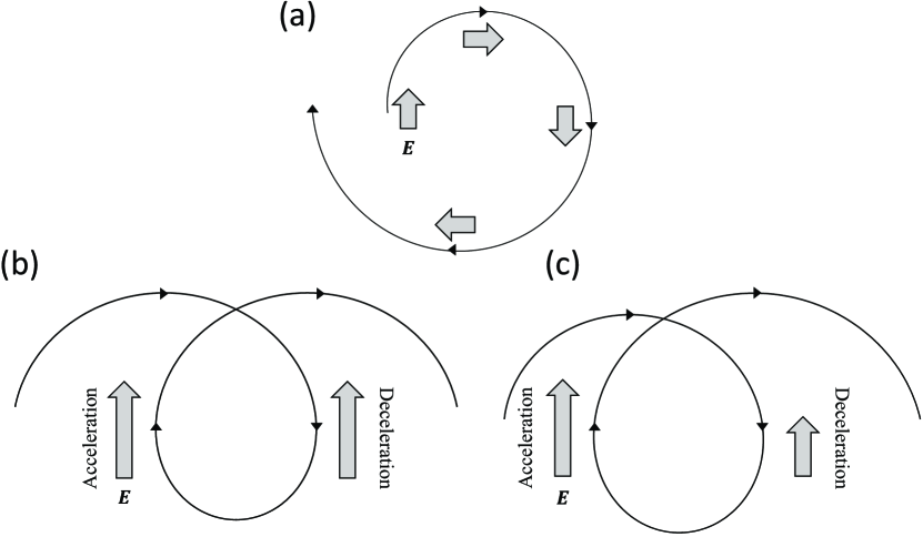
Figure 1.— Schematic pictures of the particle energy gain via interaction with MHD waves. The charge of the particle is positive. The magnetic field is perpendicular to the page, and the particle trajectories are projected to this plane. (a) Gyroresonance case ($\Omega\simeq\pm k_{\parallel}v_{\parallel}$). (b) TTD case ($v_{\parallel}\simeq\omega/k_{\parallel}$) with an Alfvén wave or a slow wave with $k_{\perp}=0$. (c) TTD case with a fast/slow wave with $k_{\perp}\neq 0$.

On the other hand, even if a particle is in the TTD resonance ($v_{\parallel}\simeq\omega/k_{\parallel}$), an Alfvén wave and a slow wave with $k_{\perp}=0$ do not accelerate the particle. In this case, the electric and magnetic fields the particle experiences are constant. As Figure 1 (b) shows, the effects of acceleration and deceleration cancel out in one gyro period. In the plane perpendicular to the magnetic field ($\bm{B}_{0}+\bm{b}$), we simply observe the $\bm{E}\times\bm{B}$ drift motion.

To increase the particle energy, a difference of the electric field in the perpendicular direction is required (see Figure 1 (c)), which means a finite parallel value of $\nabla\times\bm{E}$. From the induction equation, this condition is equivalent to a finite value of $\dot{b}_{\parallel}$, which is zero in an Alfvén wave and parallel slow/fast wave.

The energy gain per one gyro motion is $e\oint\bm{E}\cdot d\bm{l}\sim e|\Delta\bm{E}|r_{\rm L}$. The electric field difference is $|\Delta\bm{E}|\sim r_{\rm L}dE/dx_{\perp}\sim|\bm{V}\times\bm{B}_{0}|k_{\perp}r_{\rm L}/c$. During the TTD resonance, the number of gyration is roughly $N_{\rm gyro}\sim(k_{\parallel}r_{\rm L})^{-1}$, so that the energy change per interaction becomes $|e\Delta\bm{E}|r_{\rm L}N_{\rm gyro}\propto VB_{0}\tan{\theta_{k}}r_{\rm L}\propto V\tan{\theta_{k}}\gamma$. Though a lower magnetic field leads to a lower electric field, the resultant larger Larmor radius ($\propto B_{0}^{-1}$) extends the scale $\Delta x_{\perp}$, which enhances $|\Delta\bm{E}|$. Therefore, the energy change is independent of $B_{0}$, which agrees with the picture of the second order Fermi acceleration ($\Delta\gamma\propto\gamma$).

However, if $k_{\perp}r_{\rm L}\gg 1$, too frequent changes of the electric field sign in one gyro motion reduce the net energy change. To accelerate particles via the TTD resonance, the magnetic field should be strong enough to keep $k_{\perp}r_{\rm L}<1$.

3.2. Gyroresonance

The analytical description of the energy-diffusion via gyroresonance with MHD waves has been shown by many authors (see e.g., Melrose, 1974; Blandford & Eichler, 1987; Schlickeiser, 1989a, b). We do not need to review the detailed kinematics in this process. A particle of a Lorentz factor $\gamma$ interacts with mainly waves of a wavenumber

$$k_{\rm res}\equiv\frac{eB_{0}}{\gamma mc^{2}},$$ (28)

in gyroresonance.

From QLT, the diffusion coefficient with gyroresonance is represented as

$$D_{\gamma\gamma} = \frac{\pi}{12}\gamma^{2}\left(\frac{\mathcal{V}_{\rm ph}}{c}\right)^{2}\left(\frac{k_{\rm res}P_{B}(k_{\rm res})}{B_{0}^{2}}\right)\frac{eB_{0}}{\gamma mc},$$ (29)

where $\mathcal{V}_{\rm ph}$ is the phase velocity of the scattering agent. Hereafter, we express the parameter $k_{\rm min}$ as

$$k_{\rm min}=\eta\frac{eB_{0}}{mc^{2}},$$ (30)

then

$$D_{\gamma\gamma}\simeq\frac{\pi}{12}(q-1)\left(\frac{\mathcal{V}_{\rm ph}}{c}\right)^{2}\frac{\delta B^{2}}{B_{0}^{2}}\eta^{q-1}\gamma^{q}\frac{eB_{0}}{mc}.$$ (31)

From equations (15)–(17), $\delta B^{2}/B_{0}^{2}\sim(\overline{V}/\mathcal{V}_{\rm ph})^{2}$. Then, irrespectively of the wave mode, the diffusion coefficient is written as

$$D_{\gamma\gamma} \simeq \frac{\pi}{12}(q-1)\left(\frac{\overline{V}}{c}\right)^{2}\eta^{q-1}\gamma^{q}\frac{eB_{0}}{mc}$$

$$\simeq 3.76\times 10^{-7}\left(\frac{\overline{V}}{10^{-3}c}\right)^{2}\left(\frac{\eta}{10^{-2}}\right)^{2/3}\left(\frac{\gamma}{10}\right)^{5/3}\frac{eB_{0}}{mc},$$

where we have adopted $q=5/3$.

3.3. TTD Resonance

3.3.1 Resonance Broadening

The fraction of particles that fulfill the resonance condition $v_{\parallel}=\mathcal{V}_{{\rm ph},\parallel}\ll c$ is very small for the isotropic particle distribution, so that the TTD is usually ignored in QLT. The condition is rewritten as $\cos\theta_{\rm p}\sim\mathcal{V}_{{\rm ph},\parallel}/c$, where $\theta_{\rm p}$ is the pitch angle. However, even if the initial pitch angle is smaller than $\cos^{-1}{(\mathcal{V}_{{\rm ph},\parallel}/c)}$, the finite amplitude of the turbulence can change the pitch angle, and make the particles put into the TTD resonance.

The non-resonant pitch angle change comes from the mirror force. We write the initial parallel and perpendicular components of the particle velocity as $v_{\parallel,0}$ and $v_{\perp,0}$, respectively. According to $v_{\parallel}^{2}+v_{\perp}^{2}=c^{2}$ and the adiabatic invariance $p_{\perp}^{2}/B$, the fluctuating magnetic field $B_{0}+\delta B$ changes the velocity as

$$v_{\parallel}^{2}=v_{\parallel,0}^{2}-v_{\perp,0}^{2}\frac{\delta B}{B_{0}}.$$ (34)

Denoting the square of the mean amplitude of the disturbed field component as $\left<(\delta B)^{2}\right>$, we introduce the Bohm factor as

$$\xi\equiv\frac{B_{0}^{2}}{\left<(\delta B)^{2}\right>}.$$ (35)

To make particles put into the TTD resonance with non-relativistic waves ($\mathcal{V}_{{\rm ph},\parallel}\ll c$), $v_{\parallel}\simeq 0$ is required. If the initial pitch angle is larger than $\theta_{\rm min}$, which is defined as

$$\sin^{2}{\theta_{\rm min}}\equiv\frac{1}{1+\xi^{-1/2}},$$ (36)

$v_{\parallel}\simeq 0$ is realized by the mirror force.

In the isotropic distribution, the fraction of particles that satisfy $\theta_{\rm min}<\theta_{\rm p}<\pi-\theta_{\rm min}$ is

$$f_{\rm res}=\cos{\theta_{\rm min}}=\frac{1}{\sqrt{1+\xi^{1/2}}},$$ (37)

when $\cos{\theta_{\rm min}}>\mathcal{V}_{\rm ph}/c$. Note that the resonance broadening does not depend on the wave scale.

To demonstrate the resonance broadening, we provide isotropic slow-mode waves with $\nu=11/3$ ($q=5/3$) between $k=k_{\rm min}$ and $k_{\rm max}=100k_{\rm min}$, where $\eta=10^{-4}$, and inject particles with the initial Lorentz factor $10$, for which $k_{\rm res}=10k_{\rm max}$. In this case, the pitch angle diffusion due to gyroresonance can be neglected. With the method explained in §2, we follow the particle trajectory. The results are shown in Figure 2. Here, we have assumed $\alpha=10$, $\mathcal{V}_{\rm A}=10^{-2}c$, and $\overline{V}=0.1\mathcal{V}_{\rm A}$. For $\alpha\gg 1$, the phase velocity of the slow wave is roughly $\mathcal{V}_{\rm A}$, so that the Bohm factor is approximated as $\xi\simeq(\mathcal{V}_{\rm A}/\overline{V})^{2}=100$ in this case.

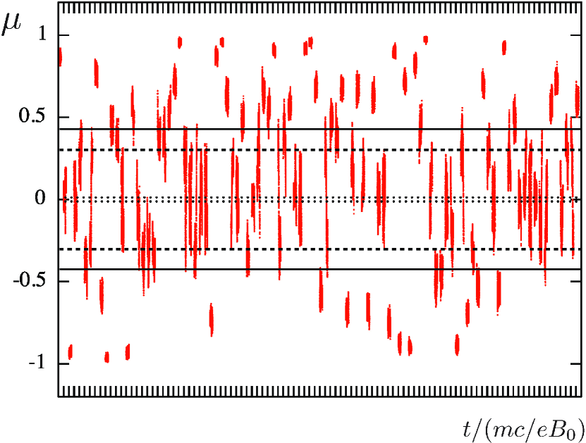
Figure 2.— Time evolution of the pitch angle of the each particles. We adopt isotropic slow-mode waves, whose parameters are $q=5/3$, $\alpha=10$, $\eta=10^{-4}$, $k_{\rm max}=100k_{\rm min}$, $\mathcal{V}_{\rm A}=10^{-2}c$, and $\overline{V}=10^{-3}c$. The vertical axis is the pitch angle cosine. We inject particles of $\gamma=10$ and follow each particle for a time interval of $10^{6}mc/(eB_{0})$, which corresponds to the grid scale on the horizontal axis. We plot the evolution of $\mu$ for randomly selected 100 particles with different time offsets. The horizontal dashed and solid lines correspond to $\cos{\theta_{\rm min}}\simeq\pm 0.3$ and $\sqrt{2}\cos{\theta_{\rm min}}$, respectively. The dotted lines are $\mu=\mathcal{V}_{\rm A}/c=\pm 0.01$, which is the TTD resonance condition without the resonance broadening.

Figure 2 shows that particles with $|\mu|=|\cos\theta_{\rm p}|$ smaller than $\cos{\theta_{\rm min}}\simeq 0.3$ (dashed line) can penetrate into the region $|\mu|<\mathcal{V}_{\rm A}/c=0.01$ (dotted line) owing to the mirror force. Note that the pitch angle starting from $\theta_{\rm p}=\theta_{\rm min}$ can become as small as $\cos\theta_{\rm p}=\sqrt{2}\cos{\theta_{\rm min}}$ (obtained from equation (34) with negative $\delta B$). Although $\xi=100$ is significantly large, the effect of the mirror force efficiently enlarges the resonance particle number. The example in Figure 2 is for the slow mode. The results for the fast mode are also similar to the slow-mode results.

Let us estimate the diffusion coefficient of the pitch angle in this case. The combination of the adiabatic constant $p_{\perp}^{2}/B$ and the energy $p_{\perp}^{2}+p_{\parallel}^{2}+m^{2}c^{2}$ provides

$$\frac{\Delta p}{\delta t}\sim\frac{p_{\perp}v_{\perp}}{2B}\nabla_{\parallel}|B_{\parallel}|\sim pv_{\perp}k_{\parallel}\frac{\delta B(k)}{B_{0}},$$ (38)

where $\delta B(k)\equiv\sqrt{kP_{\rm B}(k)}$. During the transit-time of the wave,

$$\delta t\sim\frac{1}{v_{\parallel}k_{\parallel}},$$ (39)

the pitch angle changes as

$$\Delta\mu\sim\frac{\Delta p}{p}\sim\frac{v_{\perp}}{v_{\parallel}}\frac{\delta B(k)}{B_{0}},$$ (40)

so that the resonance broadening is dominated by the largest scale for $q>1$. The pitch angle diffusion coefficient is written as

$$D_{\mu\mu}\sim\sum_{n}\frac{(\Delta\mu)^{2}}{\delta t}\sim\sum_{n}v_{\perp}^{2}k_{\parallel}^{2}\left(\frac{k_{n}P_{B}(k_{n})}{B_{0}^{2}}\right)\cdot\delta t.$$ (41)

3.3.2 Energy Diffusion Coefficient

Figure 3 shows the particle distribution in a cross section of the momentum space for the same simulation as that in Figure 2, where slow waves are isotropically propagating. As discussed in the previous subsection, particles within $|\mu|<\cos{\theta_{\rm min}}$ can resonate with the waves. We can see that only such resonating particles are exuded outside the equi-energy circle of $\gamma\sqrt{\beta_{x}^{2}+\beta_{z}^{2}}=10$, which is the initial energy at injection. In this subsection, we describe the energy-diffusion coefficient in the TTD resonance.

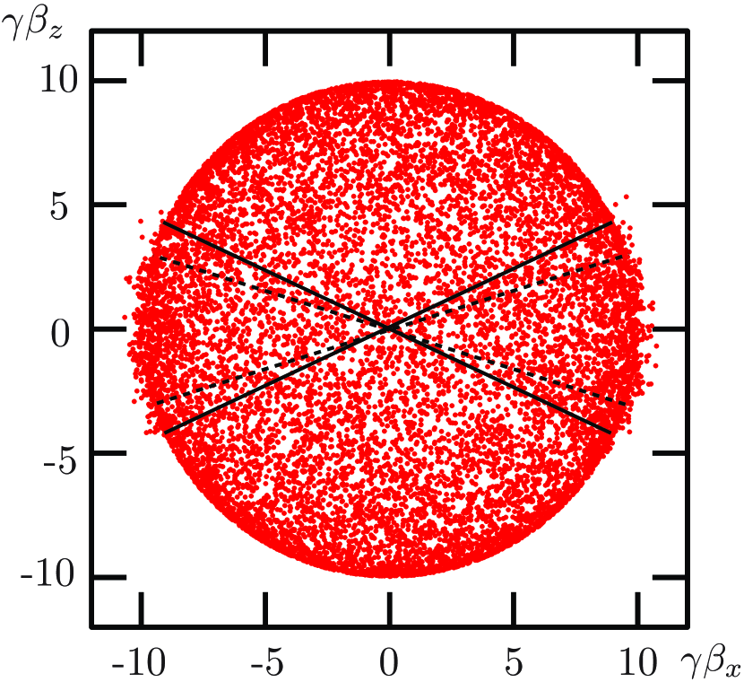
Figure 3.— Distribution of $\gamma\bm{\beta}$ of 12,800 particles after elapsed time of $10^{6}mc/eB_{0}$ in the pure slow-mode waves. The simulation is the same as that in Fig. 2. Horizontal axis is $\gamma\beta_{x}$, and vertical axis is $\gamma\beta_{z}$. The background magnetic field is parallel to $\bm{z}$. The long dashed lines and solid lines correspond to $\cos{\theta_{\rm min}}$ and $\sqrt{2}\cos{\theta_{\rm min}}$, the critera of the resonance broadening.

Figure 4 shows another demonstration of the resonance broadening for fast waves. Also in this case, the gyroresonance is negligible effect ($k_{\rm res}=10k_{\rm max}$). Though the phase velocity is faster than the phase velocity for slow wave, $\mathcal{V}_{\rm ph}/c\sim\sqrt{\alpha}\mathcal{V}_{\rm A}/c\simeq 0.03$ is still lower than $\cos{\theta_{\rm min}}\simeq 0.3$. As the figure shows, roughly 50% of particles are in the diffusion process, and rest of particles remains around the initial energy. The resonance fraction is slightly larger than the simple estimate $\cos{\theta_{\rm min}}$ or $\sqrt{2}\cos{\theta_{\rm min}}$.

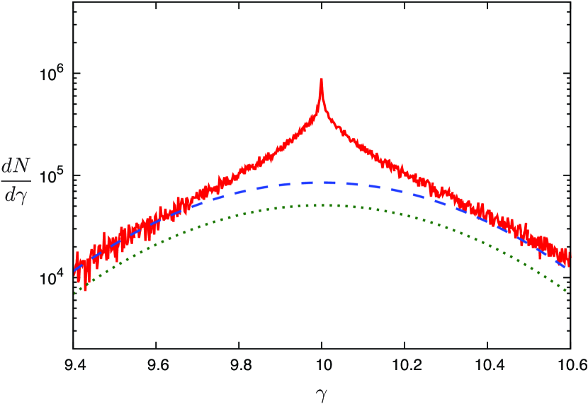
Figure 4.— Energy distribution of particles at $t=10^{6}mc/(eB_{0})$ in the pure fast-mode waves. The parameters are $q=3/2$, $\alpha=10$, $\eta=10^{-4}$, $k_{\rm max}=100k_{\rm min}$, $\mathcal{V}_{\rm A}=10^{-2}c$, and $\overline{V}=10^{-3}c$. The initial Lorentz factor is 10. The blue dashed line and green dotted lines are the Gaussian curves with dispersion $\sigma=0.5$, and particle numbers $0.5N_{\rm all}$ and $0.3N_{\rm all}$, respectively (the total particle number $N_{\rm all}=12,800$).

Because the energy-diffusion due to the TTD resonance is consistent with the second order Fermi acceleration, we can write the energy change in the timescale $\delta t\sim(v_{\parallel}k_{\parallel})^{-1}$ by considering the Lorentz transformation between the wave rest frame and Laboratory frame before and after the pitch angle change. The change of the angle $\Delta\mu$ in the wave rest frame yields the energy change as

$$\Delta\gamma\sim\frac{\mathcal{V}_{\rm ph}}{c}\gamma\Delta\mu.$$ (42)

The fraction of particle that can resonate with waves can be written as

$$f_{\rm res}=\max\left(\frac{\mathcal{V}_{\rm ph}}{c},\frac{1}{\sqrt{1+\xi^{1/2}}}\right).$$ (43)

Then, the energy-diffusion coefficient is estimated as

$$D_{\gamma\gamma}\sim\sum_{n}\frac{(\Delta\gamma)^{2}}{\delta t}f_{\rm res}\sim\sum_{n}\gamma^{2}\left(\frac{\mathcal{V}_{\rm ph}}{c}\right)^{2}\frac{(\Delta\mu)^{2}}{\delta t}f_{\rm res}.$$ (44)

From equation (41), we obtain

$$D_{\gamma\gamma}\sim\sum_{n}\gamma^{2}\left(\frac{\mathcal{V}_{\rm ph}}{c}\right)^{2}ck_{n}\left(\frac{k_{n}P_{B}(k_{n})}{B_{0}^{2}}\right)f_{\rm res}.$$ (45)

Each term in equation (45) is proportional to $k_{n}^{2-q}$, so that the largest $k_{n}$ contributes dominantly for $q<2$. As we mentioned in the previous subsection, the wave power absorption by particles is strongly suppressed for $k_{\perp}r_{\rm L}>1$. Therefore, for $k_{\rm res}<k_{\rm max}$, the diffusion coefficient is approximated as

$$D_{\gamma\gamma}\sim\gamma^{2}\left(\frac{\mathcal{V}_{\rm ph}}{c}\right)^{2}ck_{\rm res}\left(\frac{k_{\rm res}P_{B}(k_{\rm res})}{B_{0}^{2}}\right)f_{\rm res},$$ (46)

which is almost the same as the coefficient in the gyroresonance case, equation (29), except for the factor $f_{\rm res}$. Finally the expression becomes a similar equation to equation (3.2) as

$$D_{\gamma\gamma} \sim f_{\rm res}(q-1)\left(\frac{\overline{V}}{c}\right)^{2}\eta^{q-1}\gamma^{q}\frac{eB_{0}}{mc}.$$ (47)

On the other hand, for $k_{\rm res}>k_{\rm max}$, we obtain

$$D_{\gamma\gamma}\sim\gamma^{2}\left(\frac{\mathcal{V}_{\rm ph}}{c}\right)^{2}ck_{\rm max}\left(\frac{k_{\rm max}P_{B}(k_{\rm max})}{B_{0}^{2}}\right)f_{\rm res}.\\$$ (48)

From equation (27), this is rewritten as

$$D_{\gamma\gamma}\sim f_{\rm res}(q-1)\gamma^{2}\left(\frac{\overline{V}}{c}\right)^{2}ck_{\rm max}\left(\frac{k_{\rm max}}{k_{\rm min}}\right)^{1-q}.$$ (49)

The precise numerical factor for $D_{\gamma\gamma}$ may depend on the wave mode. We have derived the above rough formulation aside the concept of the resonance discussed in section 3.1. However, as we have discussed, a finite value of $k_{\perp}$ is required to change the particle energy via the TTD resonance. In the limit of $\alpha\gg 1$, the direction of fluid motion is almost parallel (perpendicular) to the wave vector $\bm{k}$ for the fast (slow) mode. For a significantly large $k_{\perp}$, the fast mode is advantageous to induce a larger electric field than the slow mode. We expect a larger energy-diffusion by the TTD resonance in the fast mode than the slow mode.

4. Diffusion Coefficients in Simulations

In this section, we show the energy-diffusion process obtained from our numerical simulations with the method explained in section 2. The injected turbulence energy at a large scale is transferred to small scale turbulences. This cascade process may be interrupted at a certain scale by energy dissipation processes like the TTD. Below this scale, the power spectrum becomes steep. This scale practically corresponds to the maximum wavenumber $k_{\rm max}$.

Hereafter, given an energy of particles, we consider two cases for the maximum wavenumber $k_{\rm max}$: one with gyroresonance ($k_{\rm res}<k_{\rm max}$) and one without gyroresonance ($k_{\rm res}>k_{\rm max}$).

4.1. With Gyroresonance

For particles of $k_{\rm res}<k_{\rm max}$, both the gyroresonance and TTD resonance contribute to the particle energy-diffusion. As shown in Figure 5, we follow the motion of $N=1,280$ particles injected with $\gamma=10$ and obtain the temporal evolution of the dispersion of $\gamma$ for each run. Between $t=10^{3}mc/(eB_{0})$ and $10^{6}mc/(eB_{0})$, we fit the evolution of the dispersion with $\left<(\Delta\gamma)^{2}\right>\propto t$ and estimate the energy-diffusion coefficient.

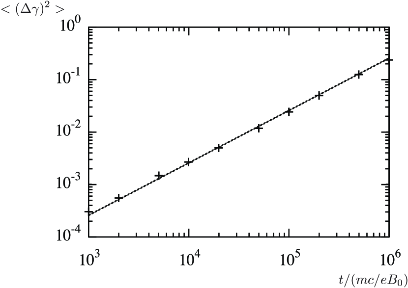
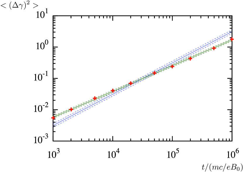
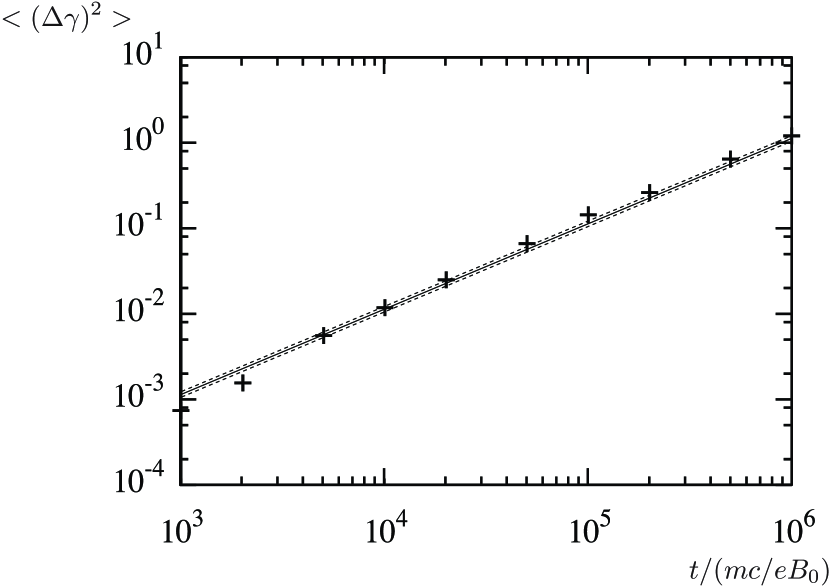
Figure 5.— Evolutions of the dispersion of Lorentz factor $\gamma$ in turbulences with $q=5/3$, $\alpha=10$, $\eta=10^{-2}$, $k_{\rm max}=100k_{\rm min}$, $\mathcal{V}_{\rm A}=10^{-2}c$, and $\overline{V}=10^{-3}c$. The initial Lorentz factor is 10 ($k_{\rm res}=0.1k_{\rm max}$). The upper, middle and lower panels show the results for pure Alfvén, fast- and slow-mode waves, respectively. The solid and dashed lines indicate the fitting results. For the Alfvén and the slow modes, the numerical results agree with the standard diffusion behavior $\left<(\Delta\gamma)^{2}\right>\propto t$. For the fast mode (middle), while the blue lines of $\left<(\Delta\gamma)^{2}\right>\propto t$ are deviated from the numerical results, the green lines of $\left<(\Delta\gamma)^{2}\right>\propto t^{0.82}$ well follow the results.

As Figure 5 shows, the dispersion for the Alfvén mode, where only the gyroresonance contributes to the energy-diffusion, precisely follow the analytical evolution as $\left<(\Delta\gamma)^{2}\right>\propto t$. We have not found signature of the advection in the energy space like the first-order Fermi acceleration, which leads to $\left<(\Delta\gamma)^{2}\right>\propto t^{2}$. However, the evolution for the fast mode significantly deviates from the standard diffusion behavior. The dispersion in the fast mode rather evolves as $\left<(\Delta\gamma)^{2}\right>\propto t^{0.82}$. Such a sub-diffusion behavior is typically seen in transient phenomena before the attainment of the steady state. The interpretation of this anomalous diffusion for the fast mode is difficult. The sub-diffusion may be due to the combination of the gyro and TTD resonances, because we observe normal diffusion behavior in cases without the gyroresonance (section 4.2). With $\xi\simeq(\mathcal{V}_{\rm A}/\overline{V})^{2}=100$, the TTD timescale is roughly written with $t_{\rm TTD}\sim\xi\gamma mc/(eB_{0})=10^{3}mc/(eB_{0})$ in our parameter set. Actually, for $t<t_{\rm TTD}$, the super-diffusion behavior ($\left<(\Delta\gamma)^{2}\right>$ evolves faster than $\propto t$) is observed in our fast-mode case. In this relatively long timescale, $t_{\rm TTD}$, the pitch angle evolution by the gyroresonance may be not diffusive under the influence of the mirror force. In spite of this anomalous behavior, we fit the numerical results with $\left<(\Delta\gamma)^{2}\right>\propto t$ as Figure 5, and obtain approximate values of the diffusion coefficient.

Table 1Diffusion coefficients with gyroresonance

Name	Mode	$q$	$D_{\gamma\gamma}/D_{\gamma\gamma,0}$
A0	Alfvén	$5/3$ (slab)	$1.08\pm 0.01$
A1	Alfvén	$5/3$	$0.35\pm 0.01$
A2	Alfvén	$3/2$	$0.41\pm 0.01$
f1	fast	$5/3$	$2.18\pm 0.31$
f2	fast	$3/2$	$2.16\pm 0.27$
s1	slow	$5/3$	$0.80\pm 0.06$
s2	slow	$3/2$	$0.68\pm 0.09$

Based on the discussion in section 3, we normalize the diffusion coefficient by an analytical estimate,

$$D_{\gamma\gamma,0}\equiv\frac{\pi}{12}(1+3f_{\rm res})(q-1)\left(\frac{\overline{V}}{c}\right)^{2}\eta^{q-1}\gamma^{q}\frac{eB_{0}}{mc}.$$ (50)

The statistical errors in Figure 5 are negligible. The errors for $D_{\gamma\gamma}$ come from the deviation from the ideal behavior $\left<(\Delta\gamma)^{2}\right>\propto t$ (see dashed lines in Figure 5). The results are tabulated in Table 1. The run A0 is the slab case, where only parallel waves are injected. In other cases, the distributions of turbulent waves are isotropic. The obtained diffusion coefficients are consistent with the analytical estimate $D_{\gamma\gamma,0}$ within a factor of 2 or 3. As we have expected in section 3.3.2, the energy-diffusion for the fast mode is slightly larger. The relatively large errors for the fast and the slow modes come from the modulated evolutions of $\left<(\Delta\gamma)^{2}\right>$ shown in Figure 5.

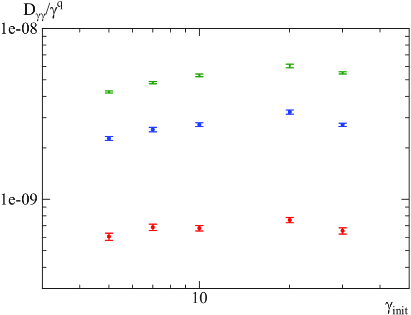
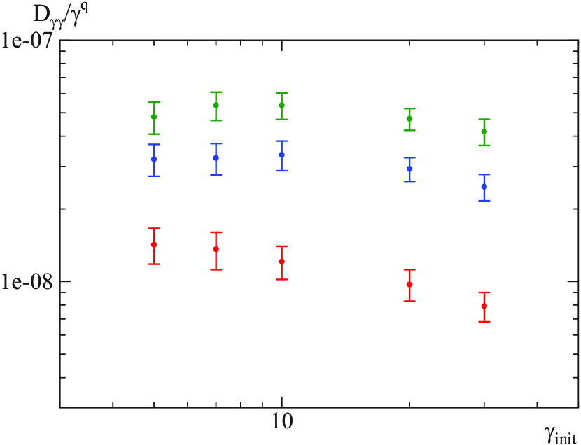
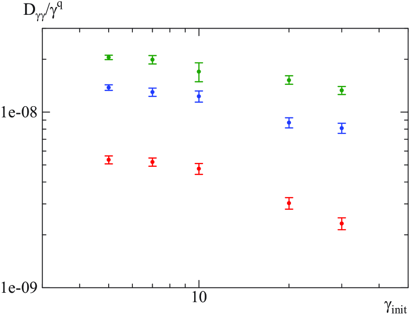
Figure 6.— Energy dependence of the diffusion coefficient for the case of $k_{\rm res}<k_{\rm max}$. The common parameters are $\alpha=10$, $\eta=10^{-2}$, $k_{\rm max}=100k_{\rm min}$, $\mathcal{V}_{\rm A}=10^{-2}c$, and $\overline{V}=10^{-3}c$. The values are normalized by $eB_{0}/(mc)$. The horizontal axis is the initial Lorentz factor. The red, blue, and green symbols correspond to $q=2$, $5/3$, and $3/2$, respectively. The upper, middle, and lower panels show the results for pure Alfvén, fast- and slow-mode waves, respectively.

To check the energy dependence $D_{\gamma\gamma}\propto\gamma^{q}$, we change the initial Lorentz factor within $k_{\rm min}<k_{\rm res}<k_{\rm max}$. The results are summarized in Figure 6. Roughly speaking, the results are consistent with the expectation $D_{\gamma\gamma}\propto\gamma^{q}$. For the slow-mode cases and the case $q=2$ in the fast mode, however, the diffusion coefficient becomes slightly lower than the anticipated values at a higher $\gamma$. At present, we do not have clear explanation for those deviations. As equation (45) indicates, $q=2$ is the threshold value above which the waves at $k=k_{\rm min}$ dominantly contribute to the TTD process rather than waves at $k=k_{\rm res}$. For $q=2$, the lower cutoff in the wavenumber spectrum may affect the energy dependence of the diffusion coefficient. In this sense, the results for the slow mode would suggest that the contribution below $k_{\rm res}$ is larger for the slow mode than the fast mode. In addition, as we have mentioned, the coexistence of the gyroresonance and TTD resonance, whose timescales are different, may cause anomalous effect on the diffusion.

4.2. Without Gyroresonance

In this subsection, we shift the wavenumber distribution toward a longer wavelength, adopting $\eta=10^{-4}$ and $k_{\rm max}=100k_{\rm min}$. For $\gamma=10$, $k_{\rm res}=10k_{\rm max}$ so that gyroresonance does not occur. We have confirmed that the energy-diffusion is not seen in the Alfvén mode. Differently from the cases with the gyroresonance, the energy dispersion evolution due to fast waves is almost diffusive ($\left<(\Delta\gamma)^{2}\right>\propto t$). For the fast and the slow modes, our results are summarized in Table 2, where we normalize the diffusion coefficient by

$$D_{\gamma\gamma,0}\equiv\frac{\pi}{4}f_{\rm res}(q-1)\gamma^{2}\left(\frac{\overline{V}}{c}\right)^{2}ck_{\rm max}\left(\frac{k_{\rm max}}{k_{\rm min}}\right)^{1-q},$$ (51)

obtained from the discussion in section 3.3.2. While the diffusion coefficients for the fast mode are slightly larger than the analytical estimate $D_{\gamma\gamma,0}$, the results for the slow mode well agree with that. The enhancement of $D_{\gamma\gamma}$ in the fast mode may be due to the relatively larger electric field induced by waves with a large $k_{\perp}$ as mentioned in section 3.3.2.

Table 2Diffusion coefficients without gyroresonance

Name	Mode	$q$	$D_{\gamma\gamma}/D_{\gamma\gamma,0}$
f3	fast	$5/3$	$5.59\pm 0.41$
f4	fast	$3/2$	$4.46\pm 0.14$
s3	slow	$5/3$	$1.13\pm 0.11$
s4	slow	$3/2$	$0.91\pm 0.09$

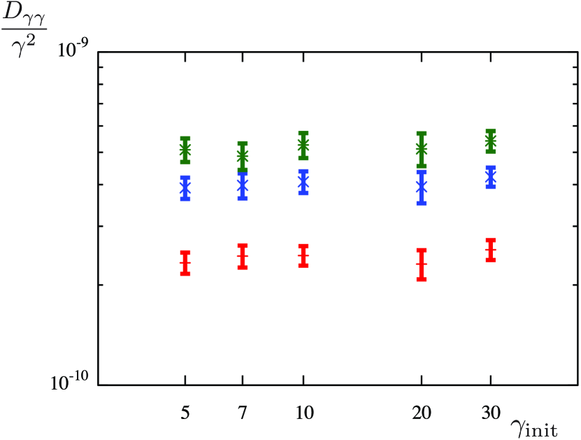
Figure 7.— Energy dependence of the diffusion coefficient for the fast-mode cases with $k_{\rm res}>k_{\rm max}$. The common parameters are $\alpha=10$, $\eta=10^{-4}$, $k_{\rm max}=100k_{\rm min}$, $\mathcal{V}_{\rm A}=10^{-2}c$, and $\overline{V}=10^{-3}c$. The horizontal axis is the initial Lorentz factor. The red, blue, and green symbols correspond to $q=2$, $5/3$, and $3/2$, respectively.

The energy dependence of the diffusion coefficients shown in Figure 7 is consistent with the hard-sphere-like acceleration irrespectively of the index $q$. The dependences on the other parameters are also shown in Figure 8. In the analytical estimate in equation (51), the diffusion coefficient does not depend on $\alpha$, but our results suggest a weak dependence on $\alpha$. For the other parameters, Figure 8 roughly supports the analytical estimate.

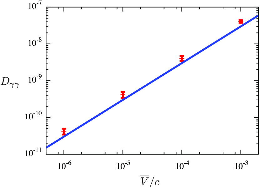
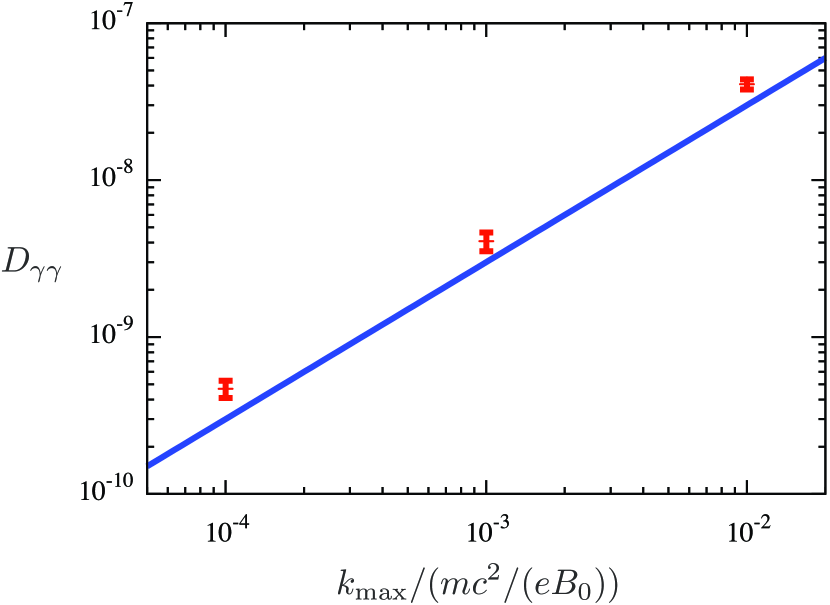
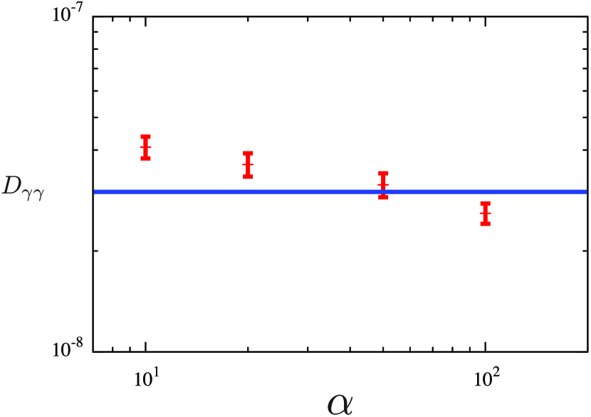
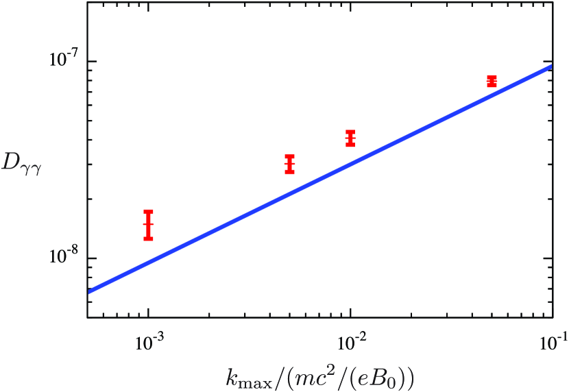
Figure 8.— Parameter dependence on the diffusion coefficient at $\gamma=10$ for the fast-mode cases with $k_{\rm res}>k_{\rm max}$. The fiducial parameters are $q=5/3$, $\alpha=10$, $\eta=10^{-4}$, $k_{\rm max}=100k_{\rm min}$, $\mathcal{V}_{\rm A}=10^{-2}c$, and $\overline{V}=10^{-3}c$. The plotted values are obtained by changing one of those parameters: (Upper left)  $\overline{V}$-dependence. The solid line shows $D_{\gamma\gamma}\propto\overline{V}^{2}$. (Upper right)  $k_{\rm max}$-dependence with a fixed $k_{\rm max}/k_{\rm min}=100$. The solid line shows $D_{\gamma\gamma}\propto k_{\rm max}$. (Lower left)  $\alpha$-dependence. The solid line shows $D_{\gamma\gamma}\propto\alpha^{0}$. (Lower right)  $k_{\rm max}$-dependence with a fixed $k_{\rm min}$. The solid line shows $D_{\gamma\gamma}\propto k_{\rm max}^{1/2}$.

5. Application of the TTD-only Model

In this paper, we have quantitatively estimated the energy-diffusion of particles via interaction with MHD waves. The combination of the effects of the acceleration and the escape from the acceleration site can produce various type of particle energy distribution (e.g. Bykov & Mészáros, 1996; Becker et al., 2006). While the gyroresonance with Alfvén waves has been frequently considered as the dominant contribution to the particle acceleration in high-energy objects (e.g. Stawartz & Petrosian, 2008; Lefa et al., 2011; Kakuwa et al., 2015), the magnetic energy in such objects is usually subdominant so that the energy of Alfvén waves seems not enough to account for the energy source of high-energy particles. Our simulations have demonstrated significant efficiency of the energy-diffusion by fast/slow waves without gyroresonance, which is not widely recognized. Such non-gyroresonance (TTD-only) interactions with compressible waves bring us an alternative picture for particle acceleration in high-energy objects.

The simple hard-sphere acceleration model without escape effect in Asano & Hayashida (2018; see also Asano & Hayashida, 2015) can reproduce various blazar spectra. As an example, let us discuss the model parameters for the representative blazar Mrk 421 in terms of the particle energy-diffusion by compressible waves without gyroresonance. In the model of Asano & Hayashida (2018), in which the broadband spectrum is reproduced with the hard-sphere acceleration, the comoving size of the acceleration/emission region $R$, the magnetic field, and the acceleration timescale $\gamma^{2}/D_{\gamma\gamma}$ are $10^{16}~{}\mbox{cm}$, $0.18~{}\mbox{G}$, and $2.1\times 10^{5}~{}\mbox{s}$, respectively. The magnetic energy density is much smaller than the electron energy density so that the turbulence energy may be dominated by fast waves.

Supersonic turbulences promptly decay via shock waves. In the relativistic outflow of Mrk 421, therefore, we can expect that the turbulence velocity is slower than the sound velocity as $\overline{V}<c/\sqrt{3}$. Adopting $\xi=1$ and $k_{\rm min}=R^{-1}$, equation (51) and Table 2 give us

$$\frac{\gamma^{2}}{D_{\gamma\gamma}}\simeq 2.1\times 10^{5}\left(\frac{\overline{V}}{0.2c}\right)^{-2}\left(\frac{k_{\rm max}^{-1}}{1.4\times 10^{12}~{}\mbox{cm}}\right)^{1/3}~{}\mbox{s},$$ (52)

for $q=5/3$. The shortest wavelength $k_{\rm max}^{-1}=1.4\times 10^{12}~{}\mbox{cm}$ corresponds to the Larmor radius of 76 TeV electron/proton, while the maximum energy of electrons in Mrk 421 is less than TeV. With a significantly large cutoff scale of the turbulence ($\gtrsim 10^{12}~{}\mbox{cm}$) and slower turbulence velocity than the sound speed, the particle acceleration required in Asano & Hayashida (2018) can be achieved. The cutoff scale $k_{\rm max}^{-1}$ may corresponds to the scale where the cascade timescale is comparable to the energy transfer timescale to non-thermal or thermal particles.

Tanaka & Asano (2017) also applied the SA models to the radio emission in the Crab nebula. In that model, parameters are time-dependent, and electrons are accelerated during initial a few hundreds years. The nebula expansion speed is $1800~{}\mbox{km}~{}\mbox{s}^{-1}$. The obtained electron spectrum is consistent with the hard radio spectrum. The required acceleration timescale (Model 2 in Tanaka & Asano, 2017) is $\gamma^{2}/D_{\gamma\gamma}\simeq 140~{}\mbox{yr}$ at the age of 100 yr, at which the size of the nebula and the magnetic field are $R_{\rm N}=5.7\times 10^{17}$ cm and $B=1.4$ mG, respectively. Assuming $q=5/3$, $\xi=1$ and $k_{\rm min}^{-1}=R_{\rm N}/10$ with equation (51) and Table 2, we consistently obtain

$$\frac{\gamma^{2}}{D_{\gamma\gamma}}\simeq 140\left(\frac{\overline{V}}{1800~{}\mbox{km}~{}\mbox{s}^{-1}}\right)^{-2}\left(\frac{k_{\rm max}^{-1}}{3\times 10^{14}~{}\mbox{cm}}\right)^{1/3}~{}\mbox{yr}.$$ (53)

The required cutoff scale of $3\times 10^{14}~{}\mbox{cm}$ is larger than the Larmor radius of electrons whose energy is less than $130$ TeV. Therefore, our estimate only with the fast-wave TTD resonance is consistent for radio-emitting particles, whose energy are typically lower than 10 GeV.

6. Discussion

In this paper, we have quantitatively estimated the energy-diffusion of particles in temporally evolving pure Alfvén, fast- or slow-mode waves. Particles can interact with waves via not only the gyroresonance but also the TTD resonance. We have confirmed the significant TTD resonance broadening due to the finite wave amplitude. If the particle Larmor radius is large enough for gyroresonance, both the gyroresonance and the TTD resonance can significantly contribute to changing the particle energy. In this case, while the coexistence of the gyroresonance and TTD resonance leads to a non-standard energy-diffusion for the fast mode, the slow-mode case is roughly consistent with the diffusion picture.

In the gyroresonance case, where the turbulence cascade develops to a smaller scale than the Larmor radius, the dominant contribution to the particle acceleration comes from waves with a scale $\sim r_{\rm L}$. Although a larger scale component can affect the particle energy with the same level, the trajectory of particles is strongly affected by smaller components than the larger scale. While we have assumed that the interaction time $\delta t$ is $1/k_{\parallel}v_{\parallel}$, it would be shortened by components with a shorter wavelength. As a result, waves with a wavelength not so far from $r_{\rm L}$ are regarded as the dominant contribution to diffuse the particle energy. Note that waves with perpendicular scales smaller than $r_{\rm L}$ do not accelerate particles efficiently (Chandran, 2000).

When the Larmor radius is shorter than the shortest wavelength, only the TTD resonance contributes to the energy-diffusion. We have demonstrated that the dominant contribution comes from the smallest scale in turbulence at $k_{\rm max}^{-1}>r_{\rm L}$ ($D_{\gamma\gamma}\propto k_{\rm max}^{2-q}$). Our simulations show a slightly larger energy-diffusion for the fast mode than the simple analytical estimate. In some high-energy objects, such as blazars, pulsar wind nebulae, and gamma-ray bursts, particle acceleration due to the TTD resonance can be expected. With $\delta B\leq B_{0}$, the energy density of Alfvén and slow-mode waves is comparable to or less than the magnetic energy density. In high-energy objects such as blazars, the magnetic energy density is estimated to be much less than the energy of the accelerated particles. In such cases, fast-mode waves are most likely the energy source of high-energy particles. The TTD-only resonance leads to the hard-sphere-like energy-diffusion coefficient, which seems consistent with blazar spectra as shown in Asano & Hayashida (2018).

To extract the essential physics, we have concentrated on the simplest cases in this paper; we have neglected the effects of wave damping, anisotropic wave distribution, and nonlinearity. Lynn et al. (2014) claimed that all scales equally contribute to accelerating particles ($D_{\gamma\gamma}\propto\ln(k_{\rm max})$) in slow waves with the resonance broadening due to wave damping. We need to distinguish the broadening mechanism in MHD simulations, which has not yet been clarified. At large scales, turbulence may be hydrodynamical eddy-turbulence rather than MHD-like wave-turbulence. In such cases, the particle acceleration mechanism by the fluid compression may be more relevant as discussed in Ptuskin (1988) and Cho & Lazarian (2006). The combination of the above multiple processes makes it difficult to extract the essential acceleration mechanism. The idealized simulations in this paper are the first step to find the dominant mechanism of the particle acceleration in turbulence.

As numerical simulations in Cho & Lazarian (2003) have shown (see also Cho et al., 2002; Kowal & Lazarian, 2010), while fast-mode waves distribute isotropically, the slow and Alfvénic turbulence is likely anisotropic, which is typically expressed by the GS model (Goldreich & Sridhar, 1995). In the GS turbulence, the perpendicular waves dominate as $k_{\parallel}\propto k_{\perp}^{2/3}$. At smaller scales than the injection scale, $k_{\perp}\gg k_{\parallel}$, in other words, eddies in small scales are elongated along the background magnetic field. Although the power-law indices of turbulence are under the discussion (Boldyrev, 2005, 2006; Beresnyak, 2014), the anisotropy is confirmed by many direct MHD simulations (for a review, Brandenburg & Lazarian, 2013).

Chandran (2000) has shown that the acceleration efficiency in the GS turbulence is much lower than that for isotropic turbulence. Even when the gyroresonance $k_{\parallel}^{-1}\sim r_{\rm L}$ is realized, the short perpendicular scale leads low efficiency of acceleration because of too frequent changes of the electric field in one gyro motion. On the other hand, the TTD resonance condition is broadened by the mirror force non-resonantly, and the GS anisotropy makes the maximum energy-absorption condition of $r_{\rm L}\sim k_{\perp}^{-1}$ at a large scale $k^{-1}\sim k_{\parallel}^{-1}\gg k_{\perp}^{-1}$, which enhances the energy-diffusion efficiency. Beresnyak et al. (2011) estimated the spatial diffusion of particles following test particles in turbulences generated from direct incompressive MHD simulations. They conclude that the main scattering process is the TTD with the pseudo-Alfvén mode, which is the incompressive limit of the slow mode, and the gyroresonance is inefficient in the GS turbulences.

In the GS turbulence, as discussed above, the TTD resonance with slow-mode waves rather than the gyroresonance with Alfvén waves dominantly contributes to the particle energy-diffusion. Considering the negative effect of the anisotropy in slow and Alfvén waves, here we again emphasize the importance of the fast mode in the particle energy-diffusion.

References

- Achternerg (1979) Achternerg, A. 1979, A&A, 76, 276
- Achternerg (1981) Achternerg, A. 1981, A&A, 98, 161
- Ackermann et al. (2016) Ackrmann, M., Anantua, R., Asano, K. et al., 2016, ApJL, 824, L20
- Asano & Hayashida (2015) Asano, K., & Hayashida, M. 2015, ApJ, 808, L18
- Asano & Hayashida (2018) Asano, K., & Hayashida, M. 2018, ApJ, 861, 31
- Asano & Mészáros (2016) Asano, K., & Mészáros, P. 2016, PRD, 94, 023005
- Asano et al. (2014) Asano, K., Takahara, F., Kusunose, M., Toma, K., & Kakuwa, J., 2014, ApJ, 780, 64
- Asano & Terasawa (2009) Asano, K., & Terasawa, T. 2009, ApJ, 705, 1714
- Asano & Terasawa (2015) Asano, K., & Terasawa, T. 2015, MNRAS, 454, 2242
- Atoyan & Aharonian (1996) Atoyan, A. M., & Aharonian, F. A. 1996, MNRAS, 278, 525
- Becker et al. (2006) Becker P. A., Le T., & Dermer C. D., 2006, ApJ, 647, 539
- Beresnyak (2014) Beresnyak, A., 2014, ApJ, 784, L20
- Beresnyak et al. (2011) Beresnyak, A., Yan, H., & Lazarian, A., 2011, ApJ, 728, 60
- Berger et al. (1958) Berger, J. M., Newcomb, W. A., Dawson, J. M., Frieman, E. A., Kulsrud, R. M., & Lenard, A. 1958, PhPl, 1, 301
- Blandford & Eichler (1987) Blandford, R., & Eichler, D. 1987, PhR, 154, 1
- Boldyrev (2005) Boldyrev, S., 2005, ApJ, 626, L37
- Boldyrev (2006) Boldyrev, S., 2006, PRL, 96, 115002
- Böttcher (1999) Böttcher, M., Pohl, M., & Schlickeiser, R., 1999, APh, 10, 47
- Brandenburg & Lazarian (2013) Brandenburg, A., & Lazarian, A., 2013, Space Science Reviews, 178, 163
- Bykov & Mészáros (1996) Bykov, A. M., & Mészáros, P., 1996, ApJ, 461, L37
- Chandran (2000) Chandran, B. D. G., 2000, PRL, 85, 4656
- Cho et al. (2002) Cho, J., Lazarian, A., & Vishniac, E. T., 2002, ApJ, 564, 291
- Cho & Lazarian (2003) Cho, J., & Lazarian, A., 2003, MNRAS, 345, 235
- Cho & Lazarian (2005) Cho, J. & Lazarian, A., 2005, Theoret. Comput. Fluid Dynamics, 2005, 19, 157
- Cho & Lazarian (2006) Cho, J. & Lazarian, A., 2006, ApJ, 638, 811
- Comisso & Sironi (2018) Comisso, L. & Sironi, L., 2018, PRL, 121, 255101
- Dmitruk et al. (2003) Dmitruk, P., Matthaeus, W. H., Seenu, N., & Brown, M. R. 2003, ApJL, 597, L81
- Fan et al. (2010) Fan, Z., Liu, S., & Fryer, C. L., 2010, MNRAS, 406, 1337