Anomalous correlators in nonlinear dispersive wave systems

Abstract

We show that Hamiltonian nonlinear dispersive wave systems with cubic nonlinearity and random initial data develop, during their evolution, anomalous correlators. These are responsible for the appearance of “ghost” excitations, i.e. those characterized by negative frequencies, in addition to the positive ones predicted by the linear dispersion relation. We use generalization of the Wick’s decomposition and the wave turbulence theory to explain theoretically the existence of anomalous correlators. We test our theory on the celebrated $\beta$-Fermi-Pasta-Ulam-Tsingou chain and show that numerically measured values of the anomalous correlators agree, in the weakly nonlinear regime, with our analytical predictions. We also predict that similar phenomena will occur in other nonlinear systems dominated by nonlinear interactions, including surface gravity waves. Our results pave the road to study phase correlations in the Fourier space for weakly nonlinear dispersive wave systems.

Keywords: Nonlinear waves , Fermi-Pasta-Ulam-Tsingou chain, Anomalous correlators

I Introduction

Wave Turbulence theory has led to successful predictions on the wave spectrum in many fields of physics Falkovich et al. (1992); Nazarenko (2011). In this framework the system is represented as a superposition of a large number of weakly interacting waves with the complex normal variables $a_{k}=a(k,t)$. In its essence, the classical Wave Turbulence theory is a perturbation expansion in the amplitude $a_{k}$ of the nonlinearity, yielding, at the leading order, to a system of quasi-linear waves whose amplitudes are slowly modulated by resonant nonlinear interactions Falkovich et al. (1992); Nazarenko (2011); Benney and Newell (1969); Newell (1968); Benney and Saffmann (1966); Kadomtsev (1965). This modulation leads to a redistribution of the spectral energy density among length-scales, and is described by a wave kinetic equation. One way to derive the wave kinetic equation is to use the random phase and amplitude approach developed in Nazarenko (2011); Choi et al. (2005, 2004). The initial state of the system can be always prepared so that the assumption of random phases and amplitudes is true. Whether the phases remain random in the evolution of the system has been an issue of intense discussions. In Wave Turbulence theory, the standard object to look at is the second-order correlator, $\langle a_{k}(t)a^{*}_{l}(t)\rangle$, where $\langle\dots\rangle$ is an average over an ensemble of initial conditions with different random phases and amplitudes. As will be clear later on, under the homogeneity assumption, the second order correlator is related to the wave action spectral density function, i.e. the wave spectrum, $n_{k}=n(k,t)$. However, one should note that the complex normal variable, as defined in the the Wave Turbulence theory, is a complex function also in physical space. Therefore, the second-order statistics are not fully determined by the above correlator. The so called “anomalous correlator”, $\langle a_{k}(t)a_{l}(t)\rangle$, see Lvov (2012); Zakharov et al. (1975), needs also to be computed. Under the hypothesis of homogeneity, will be related to the anomalous spectrum, $m_{k}=m(k,t)$, to be defined in the next Section. Indeed, if phases are totally random, this quantity would be zero. We show that, in the nonlinear evolution of the system, this is not the case. Far from it, this quantity is strongly nonzero and, in the limit of weak nonlinearity, we predict analytically and verify numerically its value.

Our ideas are based on the extension of the Wave Turbulence Theory to include these anomalous correlators. Notably, conventional Wave Turbulence Theory has been successful in the understanding of the spectral energy transfer in complex wave systems such as the ocean Janssen (2004), optics Picozzi et al. (2014) and Bose-Einstein condensates Proment et al. (2012), one dimensional chains M. Onorato and Lvov (2015), and magnets V.S.Lvov (1994). Analogously, anomalous correlators first appeared in the well known Bardeen, Cooper, and Schriffer (BCS) theory of superconductivity Bardeen (1957). Subsequently, anomalous correlators have been studied in S–theory Zakharov et al. (1975); Lvov (2012).

Recently, anomalous correlations were shown to play an important role in explaining numerical observations of nondecaying oscillations around a steady state in a turbulence–condensate system modeled by the Nonlinear Schrödinger equation Bardeen (1957, 1991, 1957). Such oscillations, corresponding to a fraction of the wave action being periodically converted from the condensate to the turbulent part of the spectrum, were shown to be directly due to phase coherence Bardeen (1957). In Guasoni et al. (2017) a system of Coupled Nonlinear Schrödinger equations has been considered and specific attention was focussed on the phenomena of recurrence of incoherent waves observed in the early stages of the dynamics. The authors derived a variant of the kinetic equation which includes anomalous correlators; the peculiarity of such an equation is that it is capable of describing properly the recurrence phenomena observed in the simulations.

One of the main tools used to derive the theory is the Wick’s contraction rule that allows one to split higher order correlators as a sum of products of second order correlators, plus cumulants. To explain analytically the existence of the anomalous correlators, it is necessary to use the more general form of the Wick’s decomposition, namely the form that allows anomalous correlators. We then demonstrate that the anomalous correlators are responsible for creating the “ghost waves”, i.e. the waves with the frequency equal to the negative of the frequency predicted by the linear dispersion relationship. These ideas are tested on a simple, but non trivial, system, i.e. the $\beta$-Fermi-Pasta-Ulam-Tsingou (FPUT) chain. The chain model was introduced in the fifties to study the thermal equipartition in crystals Fermi et al. (1955); it consists of $N$ identical masses, each one connected by a nonlinear string; the elastic force can be expressed as a power series in the displacement from equilibrium. Fermi, Pasta, Ulam and Tsingou integrated numerically the equations of motion and conjectured that, after many iterations, the system would exhibit a thermalization, i.e. a state in which the influence of the initial modes disappears and the system becomes random, with all modes excited equally (equipartition of energy) on average. Successful predictions on the time scale of equipartition have been recently obtained in M. Onorato and Lvov (2015); Pistone et al. (2018); Lvov and Onorato (2018) using the Wave Turbulence approach. In this paper we perform extensive numerical simulations with initial random data and look all at the possible excitations, once a thermalized state has been reached. This is all done by analyzing the spatial -temporal $(k-\Omega)$ spectrum, i.e. the square of the space-time Fourier transform of the wave amplitudes. Analyses of the effective dispersion relation in the nonlinear system is a well known and widely used theoretical and numerical tool, see for example Lee et al. (2013).

We give numerical evidence that in addition to the “normal” waves with frequency $\omega$ predicted by the linear dispersion relation for wave number $k$, there are the “ghost” excitations with the negative frequencies. Our theoretical analysis reveals that the origin of those “ghost” excitations resides on the nonzero values of the second-order anomalous correlator.

II The Model

The theory that we develop hereafter applies to any system with cubic nonlinearity. Examples of such systems among others, include deep water surface gravity waves  Zakharov (1968), Nonlinear Klein Gordon Pistone et al. (2018), $\beta$-Fermi-Pasta-Ulam-Tsingou chain. In normal variables $a_{k}$ the Hamiltonian of these systems assumes the canonical form:

$$\begin{split}&H=\sum_{k}{\omega_{k}|a_{k}|^{2}}+\sum_{k_{1},k_{2},k_{3},k_{4}}\big{[}(T^{(1)}_{1234}a_{1}^{*}a_{2}a_{3}a_{4}+c.c)\delta_{1}^{234}\\ &+\frac{1}{2}T^{(2)}_{1234}a_{1}^{*}a_{2}^{*}a_{3}a_{4}\delta_{12}^{34}+\frac{1}{4}T^{(4)}_{1234}(a_{1}^{*}a_{2}^{*}a_{3}^{*}a_{4}^{*}+c.c)\delta_{1234}\big{]},\end{split}$$ (1)

where $\omega_{k}=\omega(k)$ are the positive frequencies associated to the wave numbers via the dispersion relation, $T^{(i)}_{1234}$ are coefficients that depend on the problem considered and satisfy specific symmetries for the system to be Hamiltonian, $c.c.$ implies complex conjugation, $a_{j}=a(k_{j},t)$ are the complex normal variables, $\delta_{ij}^{lm}=\delta(k_{i}+k_{j}-k_{l}-k_{m})$ is the Kronecker Delta. We assume that the only resonant interactions possible are the ones for which the following two relations are satisfied for a set of wave numbers

$$k_{1}+k_{2}=k_{3}+k_{4},\;\;\;\omega(k_{1})+\omega(k_{2})=\omega(k_{3})+\omega(k_{4}).$$ (2)

With the objective of presenting some comparison with numerical simulations, out of many physical systems described by the above Hamiltonian, we select a simple one dimensional system, the $\beta$-Fermi-Pasta-Ulam-Tsingou chain. Modeling a vibrating string, this problem consists of a system of $N$ identical particles connected locally to each other by a nonlinear oscillator. In the physical space the displacements with respect to the equilibrium position $q_{j}(t)$ and their momenta $p_{j}(t)$, the Hamiltonian takes the following form:

$$H=H_{2}+H_{4}$$ (3)

with

$$\begin{split}&H_{2}=\sum\limits_{j=1}^{N}\left(\frac{1}{2}p_{j}^{2}+\frac{1}{2}(q_{j}-q_{j+1})^{2}\right),\\ &H_{4}=\frac{\beta}{4}\sum\limits_{j=1}^{N}(q_{j}-q_{j+1})^{4}.\end{split}$$ (4)

$\beta$ is the nonlinear spring coefficient (without loss of generality, we have set the masses and the linear spring constant equal to 1). The Newton’s law in physical space is given by:

$$\ddot{q}_{j}=(q_{j+1}+q_{j-1}-2q_{j})+\beta\big{[}(q_{j+1}-q_{j})^{3}-(q_{j}-q_{j-1})^{3}\big{]}.$$ (5)

We assume periodic boundary condition; our approach is developed in Fourier space and the following definitions of the direct and inverse Discrete Fourier Transforms are adopted:

$$Q_{k}=\frac{1}{N}\sum_{j=0}^{N-1}q_{j}e^{-i2\pi kj/N},\;q_{j}=\sum_{k=-N/2+1}^{N/2}Q_{k}e^{i2\pi jk/N},$$ (6)

where $k$ are discrete wave numbers and $Q_{k}$ are the Fourier amplitudes. The displacement $q_{j}$ and momentum $p_{j}$ of the $j$ particle are linked by canonically conjugated Hamilton equations

$$\dot{p}_{j}=-\frac{\partial H}{\partial q_{j}},\dot{q}_{j}=\frac{\partial H}{\partial p_{j}}.$$

We then perform the Fourier transformation to Fourier images of position and momenta, and then additional canonical transformation to complex amplitude $a_{k}$ given by

$$a_{k}=\frac{1}{\sqrt{2\omega_{k}}}(\omega_{k}Q_{k}+iP_{k}),$$ (7)

where $\omega_{k}=2|\sin(\pi k/{N})|>0$ and $Q_{k}$ and $P_{k}$ are the Fourier amplitudes of $q_{j}$ and $p_{j}$, respectively. In terms of $a_{k}$ the equation of motion reads, see Bustamante et al. (2019):

$$\begin{split}&i\frac{da_{1}}{dt}=\omega_{k_{1}}a_{1}+\sum_{k_{2},k_{3},k_{4}}\big{(}T^{(1)}_{1234}a_{2}a_{3}a_{4}\delta_{1}^{234}+T^{(2)}_{1234}a_{2}^{*}a_{3}a_{4}\delta_{12}^{34}+\\ &+T^{(3)}_{1234}a_{2}^{*}a_{3}^{*}a_{4}\delta_{123}^{4}+T^{(4)}_{1234}a_{2}^{*}a_{3}^{*}a_{4}^{*}\delta_{1234}\big{)},\end{split}$$ (8)

where all wave numbers $k_{2},k_{3}$ and $k_{4}$ are summed from $0$ to $N-1$ and $\delta_{ab..}^{cd..}=\delta(k_{a}+k_{b}+...-k_{c}-k_{d}-...)$ is the generalized Kronecker Delta that accounts for a periodic Fourier space, i.e. its value is one when the argument is equal to 0 (mod $N$). The matrix elements $T^{(1)}_{1234}$, $T^{(2)}_{1234}$, $T^{(3)}_{1234}$, prescribe the strength of interactions of wave numbers $k_{1}$, $k_{2}$, $k_{3}$ and $k_{4}$. Their values (30) are given in Appendix A.

II.1 The $(k-\Omega)$ spectrum

The main statistical object discussed in this paper is the wave number-frequency $(k-\Omega)$ spectrum. Starting from the complex amplitude $a(k,t)$ we take the Fourier transform in time so that we get $a(k,\Omega)$; Under the hypothesis of homogeneous and stationary conditions, the second-order $(k-\Omega)$ correlator takes the following form

$$\langle a(k_{i},\Omega_{p})a(k_{j},\Omega_{q})^{*}\rangle=N(k_{i},\Omega_{p})\delta(k_{i}-k_{j})\delta(\Omega_{p}-\Omega_{q}),$$ (9)

where $\langle....\rangle$ implies averages over initial conditions with different random phases. $N(k,\Omega)$ is the $(k-\Omega)$ spectrum defined as follows:

$$N^{(a)}(k,\Omega)=\frac{1}{2\pi}\frac{1}{N}\int_{-\infty}^{+\infty}\sum_{l=1}^{N}R(l,\tau)\mathrm{e}^{-i2\pi kl/N}\mathrm{e}^{-i\Omega\tau}d\tau,$$ (10)

with $R(l,\tau)=\langle a_{j}(t)^{*}a_{j+l}(t+\tau)\rangle$ is the space-time autocorrelation function.
The linear $(k-\Omega)$ spectrum - Before diving into the nonlinear dynamics, we discuss the predictions in the linear regime. Therefore, we start by neglecting the nonlinearity in equation (8) and find the solution in the form

$$\begin{split}a_{k}(t)=a_{k}(t_{0})e^{-i\omega_{k}t}.\end{split}$$ (11)

where $t_{0}$ is a time at which the solution is known or an initial condition. We then take Fourier transform in time

$$\begin{split}a(k,\Omega)=a(k,t_{0})\delta(\Omega-\omega_{k})\end{split}$$ (12)

After multiplication by its complex conjugate and taking averages over different realizations with the same statistics, we get:

$$N^{(a)}(k,\Omega)=n^{(a)}(k,t_{0})\delta(\Omega-\omega_{k}),$$ (13)

where $n^{(a)}(k,t_{0})$ is the standard wave spectrum at time $t_{0}$ related to the second-order correlator as

$$\langle a(k_{i},t_{0})a(k_{i},t_{0})^{*}\rangle=n^{(a)}(k_{i},t_{0})\delta(k_{i}-k_{j}).$$ (14)

and defined via the autocorrelation function as

$$n^{(a)}(k_{i},t_{0})=\frac{1}{N}\sum_{l}\langle a_{j}(t_{0})a_{j+l}(t_{0})^{*}\rangle e^{-i2\pi kl/N}.$$ (15)

In the linear regime $n^{(a)}(k_{i},t_{0})$ does not evolve in time.

Equation (13) implies that in the linear case the $(k-\Omega)$ spectrum is different from zero only for those values of $\Omega$ and $k$ for which the dispersion relation is satisfied. Note that in this formulation $\omega_{k}$ is defined as a positive quantity; therefore, only the positive branch of the dispersion relation curve appears in the linear regime.

II.2 Numerical results for the $(k-\Omega)$ spectrum

We now test the predictions from equation (13) both in the linear regime and observe what happens to it in the nonlinear regime. We perform numerical simulations of the equations (5) using a symplectic algorithm, see Yoshida (1990). We use 32 particles in the simulations; such choice is completely uninfluential for the results presented below. In the linear regime, we just prescribe a thermalized spectrum with some initial random phases of the wave amplitudes $a_{k}$ and evolve the system in time up to a desired final time; a Fourier Transform in time is then taken to build the $(k-\Omega)$ spectrum. In the nonlinear regime we perform long simulations up to a thermalized spectrum. For a given nonlinearity, 1000 realizations characterized by different random phases are made and ensemble averages are considered to compute the $(k-\Omega)$ spectrum. All simulations have the same initial linear energy and, from an operative point of view, the only difference between them is the value of $\beta$. To characterize the strength of the nonlinearity, we use the following ratio between nonlinear and linear Hamiltonians at the beginning of each simulation:

$$\epsilon=\frac{H_{4}}{H_{2}}\propto\beta$$ (16)

Results are shown in Figure 1, where, for different values of the nonlinear parameter $\epsilon$, the spectrum $N^{(a)}(k,\Omega)$ is plotted using a colored logarithmic scale. We first focus our attention on the linear regime, $\epsilon=0$: results are shown in Figure 1(a).

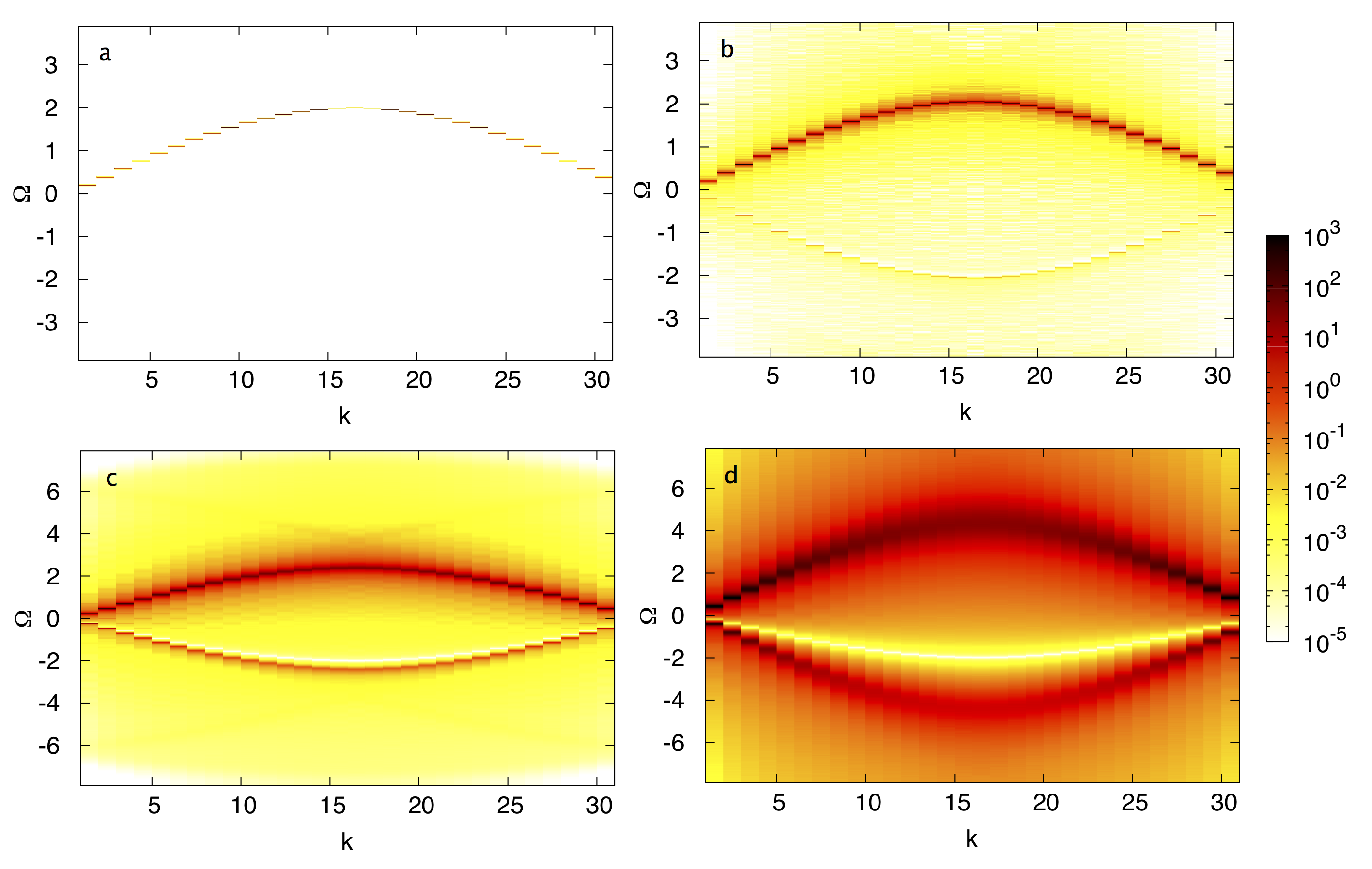
Figure 1: $(k-\Omega)$ spectrum, $N^{(a)}(k,\Omega)$, for different values of $\epsilon$: $(a)$ $\epsilon=0$, $(b)$ $\epsilon=0.0089$ $(c)$ $\epsilon=0.089$ $(d)$ $\epsilon=1.12$. In the linear case, $(a)$, the $N^{(a)}(k,\Omega)$ is different from 0 only when the frequency $\Omega$ matches the linear dispersion relation. As the nonlinearity is increased, $(b-d)$, a frequency shift, a broadening of the frequencies and a lower branch less intense than the upper one are visible. Waves with negative frequencies are named “ghost” excitations.

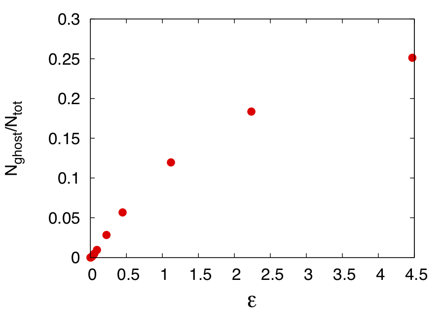
Figure 2: Ratio between the number of “ghost” excitations, $\text{N}_{\text{ghost}}$, over the total number of waves, $\text{N}_{\text{tot}}$,as a function of the nonlinearity.

As well predicted by the theory, the plot shows dots in the positive frequency plane, where the frequencies $\Omega$ and wave numbers $k$ satisfy the linear dispersion curve $\omega_{k}$. Increasing the nonlinearity, Figures 1 -(b,c,d), two well known effects appears: the first one is a shift of the frequencies, due to nonlinearity (this is more evident in Figures 1 -(c,d) where the frequency scale in the vertical axes has been changed). The second one is the broadening of the frequencies; this is related to the fact that the amplitude for each wave number is not constant in time; therefore, the amplitude-dependent frequencies are not constant in time and they oscillate around a mean value with some fluctuations. Those results are well understood, at least in the weakly nonlinear regime, and can be predicted using Wave Turbulence tools, see Nazarenko (2011); Lvov and Onorato (2018). Besides these two effects, starting from Figure 1-(b), the presence of a lower branch, whose intensity is much less than the upper one, starts to be visible. The lower curve becomes more important and, when the nonlinearity is of order one, is of the same order of magnitude of the upper one. The total number of waves in the simulation, $\text{N}_{\text{tot}}$, is given by the integral over $\Omega$ and the sum over all $k$ of the function $N^{(a)}(k,\Omega)$. In the weakly nonlinear regime, $\text{N}_{\text{tot}}$ is an adiabatic invariant of the equation of motion (5); the plot highlights the existence of waves with negative frequencies, which will be named “ghost” excitations. One of the scopes of the present paper is the understanding of the origin of such waves. Before entering into the discussion, we show in Figure 2 the ratio of “ghost” excitations, $\text{N}_{\text{ghost}}$, i.e. $N^{(a)}(k,\Omega)$ integrated over negative frequencies and summed over all wave numbers, divided by the total number of waves, $\text{N}_{\text{tot}}$. As can be seen from the plot, there is a monotonic growth of the “ghost” waves that, for very large nonlinearity, can reach values up to 25$\%$ of the total number.

III Anomalous correlators

To explain the presence of “ghost” excitations, we introduce the so called second-order anomalous correlator Lvov (2012); Zakharov et al. (1975); Guasoni et al. (2017):

$$\langle a_{k}(t)a_{j}(t)\rangle=m_{k}(t)\delta(k+j),$$ (17)

with the anomalous spectrum defined as

$$m_{k}^{(a)}(t)=\frac{1}{N}\sum_{l}\langle a_{j}a_{j+l}\rangle e^{-i2\pi kl/N}.$$ (18)

Similarly, we also introduce the second-order $(k-\Omega)$ anomalous correlator:

$$\langle a(k_{i},\Omega_{l})a(k_{j},\Omega_{m})\rangle=M^{(a)}(k_{i},\Omega_{l})\delta(k_{i}+k_{j})\delta(\Omega_{l}+\Omega_{m}),$$ (19)

where

$$M^{(a)}(k,\Omega)=\frac{1}{2\pi}\frac{1}{N}\int_{-\infty}^{+\infty}\sum_{l=1}^{N}S(l,\tau)\mathrm{e}^{-i2\pi kl/N}\mathrm{e}^{-i\Omega\tau}d\tau$$ (20)

and $S(l,\tau)=\langle a_{j}(t)a_{j+l}(t+\tau)\rangle$. The presence in equations (17) and (19) of the Kronecker $\delta$ over wave numbers and the Dirac $\delta$ over frequency, are related to the hypothesis of statistical homogeneity and stationarity, respectively. Note that $M^{(a)}(k,\Omega)$ is not the Fourier transform in time of $m_{k}^{(a)}(t)$ and in general both can be complex functions.

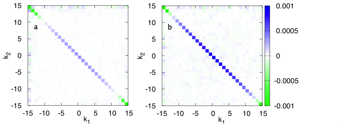
Figure 3: The real part of the second-order anomalous correlator, ${\text{R}e}[\langle a_{k_{1}}a_{k_{2}}\rangle]$, for (a) $\epsilon=0.0089$, (b) $\epsilon=1.12$. A diagonal contribution corresponding to $k_{2}=-k_{1}$ is evident in both figures. As the nonlinearity is increased, the contribution becomes larger.

To verify numerically that the anomalous correlator is indeed nonzero, we measure numerically the real part of the second-order correlator $\langle a_{k_{i}}(t)a_{k_{j}}(t)\rangle$ as a function of $k_{1}$ and $k_{2}$. Results are plotted in Figure 3 where we show the results of two numerical simulations characterized by two different values of the nonlinear parameter, (a) $\epsilon=0.0089$ and (b) $\epsilon=1.12$. In both cases, a diagonal contribution is visible, pointing out the existence of anomalous correlators in the $\beta$-FPUT model.

Generalization of the Wick’s decomposition - Using (17), it is straightforward to extend the Wick’s decomposition by taking into account the anomalous correlators, as done in V.S.Lvov (1994):

$$\begin{split}&\langle a_{k}^{*}a^{*}_{l}a_{p}a_{n}\rangle=n_{k}n_{l}(\delta^{k}_{p}\delta^{l}_{n}+\delta^{k}_{n}\delta^{l}_{p})+m^{*}_{k}m_{p}\delta_{kl}\delta_{pn},\\ &\langle a_{k}^{*}a_{l}a_{p}a_{n}\rangle=n_{k}m_{p}(\delta_{k}^{l}\delta_{pn}+\delta_{k}^{n}\delta_{lp})+n_{k}\delta^{p}_{k}m_{l}\delta_{nl},\\ &\langle a_{k}a_{l}a_{p}a_{n}\rangle=m_{k}m_{l}(\delta_{kp}\delta_{ln}+\delta_{kl}\delta_{pn}+\delta_{kl}\delta_{pn}).\end{split}$$ (21)

The above relations will be fundamental for making a natural closure of the moments when calculating analytically the $(k-\Omega)$ spectrum.

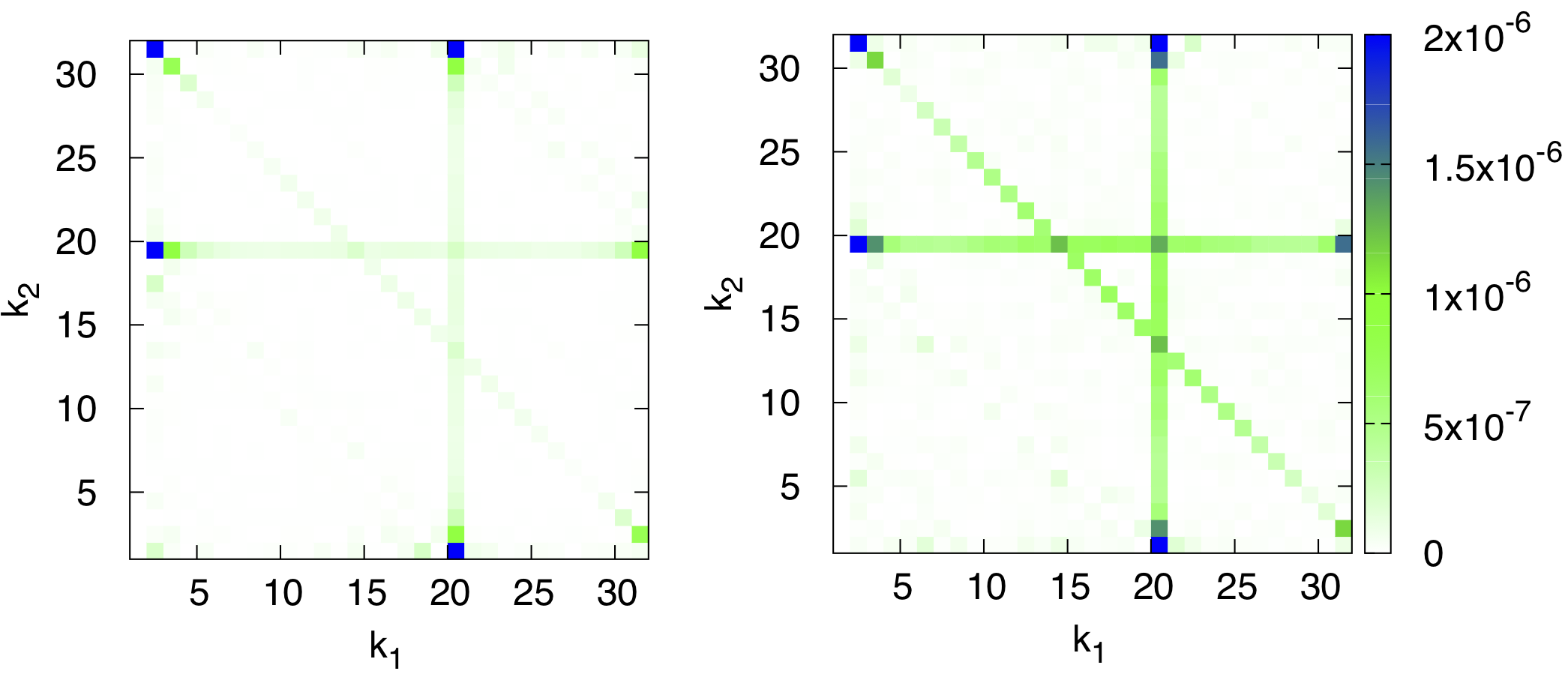
Figure 4: Fourth-order correlator $|{\text{R}e}[\langle a_{k_{1}}a_{k_{2}}a_{k_{3}}^{*}a_{k_{1}+k_{2}-k_{3}}^{*}\rangle]|$ with $k_{3}$=20. (a) $\epsilon=0.0089$, (b) $\epsilon=1.12$. Different horizontal, vertical and diagonal lines are visible. Horizontal and vertical lines corresponds to trivial resonances: $k_{1}=k_{3}$, vertical line; $k_{2}=k_{3}$, horizontal line; $k_{2}=-k_{1}+N$, diagonal line. The latter line corresponds to the presence of an anomalous second-order correlator. The intensity of the lines is larger for larger nonlinearity.

In Figure 4, we find further evidence justifying this decomposition by plotting the real part of the fourth-order correlator $\langle a_{k_{1}}a_{k_{2}}a_{k_{3}}^{*}a_{k_{1}+k_{2}-k_{3}}^{*}\rangle$ with $k_{3}=20$, computed from numerical simulations for (a) $\epsilon=0.0089$ and (b) $\epsilon=1.12$. The diagonal lines in both figures, highlighting the contribution from the second-order anomalous correlator, are noticeable. The vertical and horizontal lines correspond to the trivial resonances in which two wave numbers are equal (mod $N$).

III.1 Theoretical prediction for the anomalous correlator in the weakly nonlinear regime

A key step for the development of a theory for the anomalous correlator is the change of variable (near identity transformation) which allows one to remove bound modes, i.e. those modes that are phase locked to free modes and do not obey the linear dispersion relation. The procedure is well known in Hamiltonian mechanics and well documented for example in Falkovich et al. (1992). We accomplish this via the following canonical transformation from variable $a_{k}(t)$ to $b_{k}(t)$

$$\begin{split}&a_{1}=b_{1}+\sum\limits_{k_{2},k_{3},k_{4}}\big{[}B^{(1)}_{1234}b_{2}b_{3}b_{4}\delta^{234}_{1}+B^{(3)}_{1234}b_{2}^{*}b^{*}_{3}b_{4}\delta^{4}_{123}+\\ &+B^{(4)}_{1234}b^{*}_{2}b^{*}_{3}b^{*}_{4}\delta_{1234}\big{]},\end{split}$$ (22)

with the coefficients $B^{(i)}_{1234}$ selected in such a way to remove non resonant terms in the original Hamiltonian Krasitskii (1994). Their values are given in Appendix A.

The transformation is asymptotic in the sense that the small amplitude approximation is made and the terms in the sums on the right hand side are much smaller than the leading order term $b_{1}$. The evolution equation for variable $b_{k}(t)$ contains resonant interactions and take the following standard form:

$$\begin{split}i\frac{db_{1}}{\partial t}=\omega_{1}b_{1}+\sum_{k_{2},k_{3},k_{4}}T^{(2)}_{1234}b_{2}^{*}b_{3}b_{4}\delta_{12}^{34}+{\text{h.o.t.}}\end{split}$$

where higher order terms arising from the transformation have been neglected.

Using the transformation (22) and the generalized Wick’s decomposition (21), we can now build the time averaged anomalous spectrum (for details, see Appendix B):

$$\begin{split}&\langle m_{k}^{(a)}(t)\rangle_{t}=2\left(n_{k}^{(a)}+n_{-k}^{(a)}\right)\sum_{j}B^{(3)}_{k,-k,j,j}n_{j}^{(a)},\end{split}$$ (23)

where $\langle...\rangle_{t}$ implies averaging over time. For the $\beta$–FPUT system in thermal equilibrium, where $n^{(a)}_{k}=T/\omega_{k}$ with $T$ constant, (23) reduces to

$$\omega_{k}|\langle m_{k}^{(a)}(t)\rangle_{t}|=\frac{3NT^{2}\beta}{2}.$$ (24)

In Figure 5 we compare this prediction for $\omega_{k}|\langle m_{k}^{(a)}(t)\rangle_{t}|$ in thermal equilibrium to the values given by numerical simulations for varying values of nonlinearity: the results are in good agreement in the weakly nonlinear regime, $\epsilon<0.1$ Here 500 ensembles were used to build the correlator $m_{k}(t)$; the subsequent time averaging window used was $10^{5}$ with a sample spacing of $\Delta t=0.1$. For larger nonlinearity, is expected that higher order terms play a role in the evolution of the anomalous correlator.

In Figure 6 we show the time evolution of the first five modes of $|\langle\omega_{k}m_{k}^{(a)}(t_{a})\rangle_{t_{a}<t}|$, where ensemble averaging is used to build $m_{k}^{(a)}(t)$ and time averaging is used over the window $0<t_{a}<t$ to remove fast oscillations (see equation (36)). We verify that this quantity is indeed initially zero due to the randomness of phases. Here we use a larger value of nonlinearity $\epsilon=10$ to show the development of the anomalous correlator in a shorter time window. The amplitudes were initialized so that $|a_{k}(t=0)|=\sqrt{\frac{N-k}{2}}$ for $k=\pm 1,\pm 2,\pm 3$, with higher modes zero. The phases were initially normally distributed. We observe that the anomalous correlator grows with time, reaching a peak in modes 1, 2, 3, before it eventually saturates between all modes equally, with $\omega_{k}|\langle m^{(a)}_{k}(t_{a})\rangle_{t<t_{a}}|$ being constant for large times, as expected from our prediction (23).

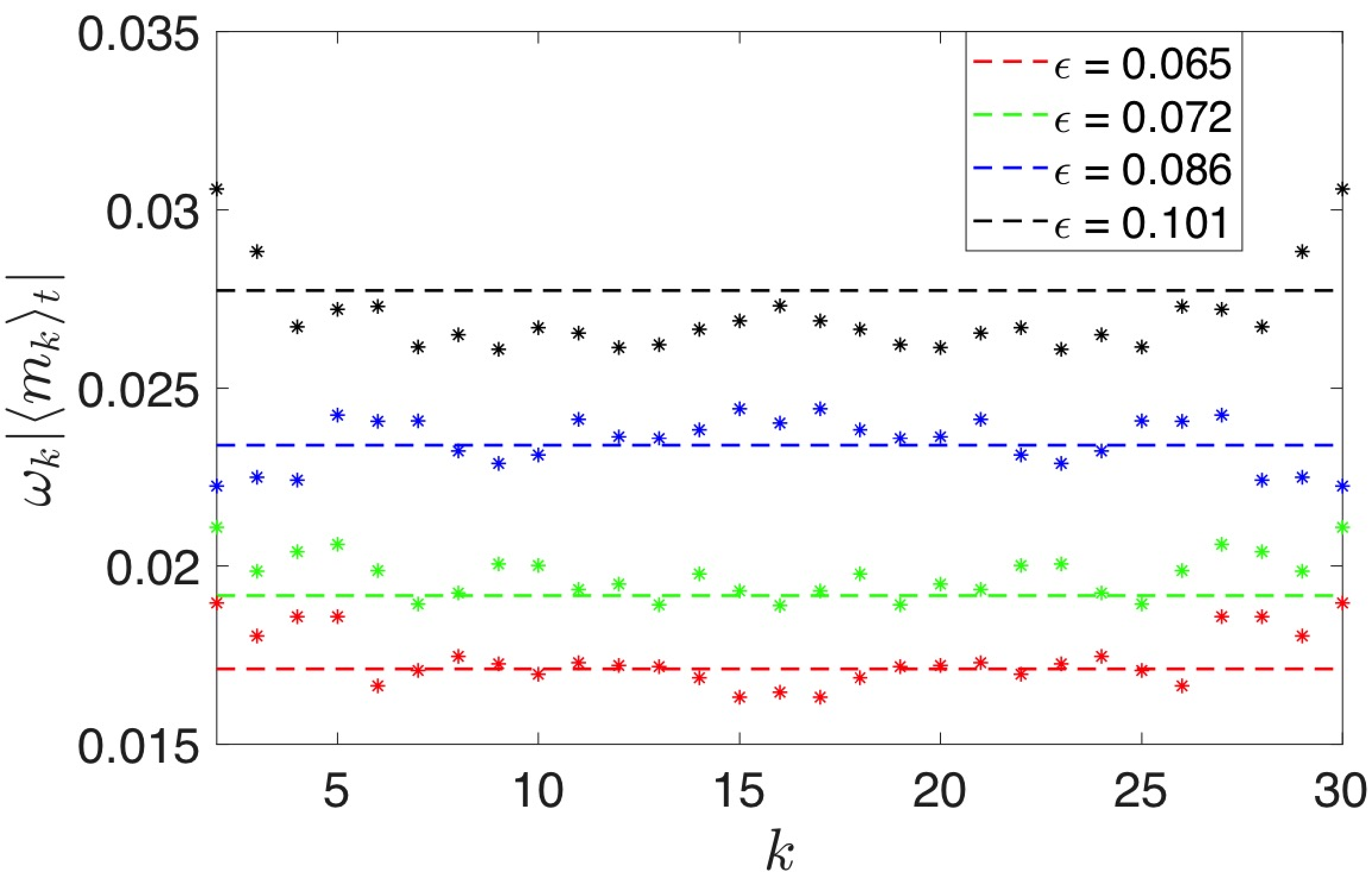
Figure 5: Comparison of anomalous spectrum $\omega_{k}|\langle m^{(a)}_{k}(t)\rangle_{t}|$ as observed in numerical simulations (dots) with theoretical predictions given by (24) (dashed lines) for $\epsilon=0.065,0.072,0.086,0.101.$

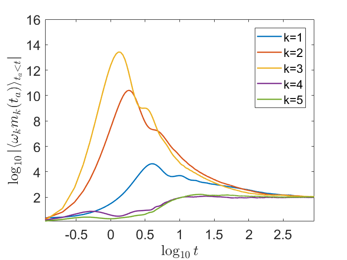
Figure 6: Time evolution of the first five modes of the averaged quantity $|\langle\omega_{k}m_{k}^{(a)}(t_{a})\rangle_{t_{a}<t}|$ from $t=0$ to $t=1000$, with $\epsilon=10$.

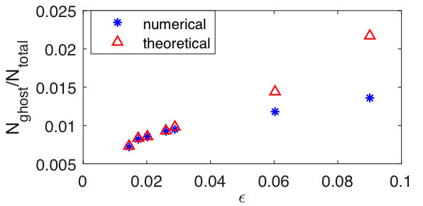
Figure 7: The ratio between the number of “ghost” excitations, $\text{N}_{\text{ghost}}$, over the total number of waves, $\text{N}_{\text{tot}}$, as a function of the nonlinearity. Numerical values are blue; theoretical values, red triangles, are given by (27).

IV Theoretical prediction for “ghost” excitations

We have now developed all the tools for predicting analytically the $(k-\Omega)$ spectrum as defined in the equation (9). Taking the Fourier Transform in time of the canonical transformation (see appendix C), using the generalized Wick’s decomposition and the hypothesis of statistical stationarity and homogeneity, we get at leading order:

$$\begin{split}N^{(a)}(k,\Omega)=&n^{(b)}(k,t_{0})\delta(\Omega-\omega_{k})+\\ &+F(k){\rm Re}[m^{(b)}(k,t_{0})]\delta(\Omega+\omega_{k})\end{split}$$ (25)

with

$$\begin{split}&F(k)=4\int\sum_{l}B_{klkl}^{(3)}N^{(b)}(l,\Omega_{p})d\Omega_{p},\end{split}$$ (26)

where we have used the fact that at the leading order $m^{(b)}(k,t)\simeq m^{(a)}(k,t)$ and $n^{(b)}(k,t_{0})\simeq n^{(a)}(k,t_{0})$. The equation (25) predicts the presence of the upper and lower branch in the $(k-\Omega$) plane. The presence of “ghost” excitations is clearly related to the second-order anomalous correlator. We can now predict the percentage of “ghost” excitations as

$$\frac{\text{N}_{\text{ghost}}}{\text{N}_{\text{tot}}}=\frac{\sum_{k}{\rm Re}[m^{(a)}(k,t_{0})]F(k)}{\sum_{k}\big{(}n^{(a)}(k,t_{0})+{\rm Re}[m^{(a)}(k,t_{0})]F(k)\big{)}}$$ (27)

In Figure 7 we plot the ratio as determined by (27) compared with the ratio observed in our simulations for several values of nonlinearity. We find that the results agree for small values of nonlinearity $\epsilon<0.03$; for larger nonlinearity the theoretical prediction is considerably larger.

V Nonlinear standing waves

The development of a regime characterized by an anomalous spectrum corresponds to a tendency for the system to develop standing waves in the original displacement variable $q_{j}(t)$. Indeed, the existence of an anomalous spectrum implies a correlation between positive and negative wave numbers. The connection between the anomalous correlator and standing waves can be seen on the following illustrative example. Consider the restrictive ensemble of realizations of the linear system where amplitudes and phases are initiated in Fourier space with a correlation between wave numbers $k=1$ and $k=-1$. Namely, let us initialize the system with amplitudes are equal and phases given by

$$a_{k}(t=0)=\begin{cases}A_{1}e^{-i\phi_{1}},&\text{if }k=1\\ A_{1}e^{i\phi_{1}},&\text{if }k=-1\\ 0,&\text{otherwise},\end{cases}$$ (28)

with the random phase $\phi_{1}$. In terms of the displacement variables this would correspond to the system being initially at rest and displaced from equilibrium as a single wave

$$q_{j}(t=0)=2A_{1}\sqrt{\frac{2}{\omega_{1}}}\cos\Big{(}\frac{2\pi j}{N}-\phi_{1}\Big{)}.$$

Since the system is assumed to be linear, the time evolution of complex amplitudes $a_{1}$ and $a_{-1}$ will be given by

$$a_{\pm 1}(t)\simeq A_{1}e^{-i(\omega_{1}t\pm\phi_{i})}.$$

Averaging over random phase $\phi_{1}$, the anomalous correlator becomes

$$m_{1}=\langle a_{1}a_{-1}\rangle=A_{1}^{2}e^{-2i\omega_{1}t},$$

analogous to the oscillating term of equation (36) for the anomalous correlator in the nonlinear case with amplitudes and phases being initially completely random. In terms of displacement, such initial conditions give

$$q_{j}(t)=2A_{1}\sqrt{\frac{2}{\omega_{1}}}\cos\Big{(}\frac{2\pi j}{N}-\phi_{1}\Big{)}\cos(\omega_{1}t),$$

which corresponds to the standing wave pattern. Thus, we see that the phase and amplitude correlations which result in a nonzero anomalous correlator are directly linked to the formation of standing waves in this particular example.

This consideration can be generalized for the case of weakly nonlinear systems and more general initial conditions. Indeed, for weakly nonlinear systems the amplitudes $|a_{1}|$ and $|a_{-1}|$ will be changing slowly over many oscillations, thus maintaining strongly nonzero anomalous correlator and standing waves.

In Figure 8-(a) we numerically solve the equations of motion with initial conditions given by (28). Here we plot a colormap of the displacement $q_{j}(t)$ for all masses as a function of time as the system reaches the timescale required for statistical thermal equilibrium. The nonlinearity parameter $\epsilon=4.74$, in the regime of strong nonlinearity and outside the regime of validity of our theory. Nevertheless, we initially consider this example to display how the system behaves when the phase correlations develop rapidly. The existence of several regions of standing wave behavior are clearly visible as darker regions in the image, as the inset Figure 8-(b) shows.

It is important to emphasize that Figure 8 shows a single realization of the system, while correlators $m_{k}(t),n_{k}(t)$ describe statistical ensemble–averaged quantities. Thus the existence of the standing wave patterns is not in violation of the presumed assumption of spatial homogeneity.

Below we give numerical evidence that such coherent structures can also be observed for smaller values of nonlinearity that are within the regime of validity of our theory.

In Figure 9-(a) we plot the displacement as a function of time for the system with $\epsilon=0.02$, a value of nonlinearity well within the regime of agreement of our theory as shown in Figures 7, 5. Here, we prescribe initial conditions so that the total energy is initially in the first wave number, i.e. $a_{k}(t=0)=0$ for all $k\neq 1$, and plot a single realization. This corresponds to a pure traveling wave solution in the linear system; indeed as seen in Figure 9-(a), the system is initially a traveling wave, represented by series of slanted parallel lines in the colormap of $q_{j}(t)$. Conversely, in Figure 9-(b) we show that by the time the system has reached the timescale required for statistical thermal equilibrium, a prominent standing wave has developed, due to the phase correlations between positive and negative lowest wave numbers. Notably, phase correlations are not restricted to only the lowest wave numbers. To emphasize this, we consider the following spatial frequency filter applied to the displacement

$$\tilde{q}_{j}(t)=\sum_{k=-N/2+1}^{N/2}H_{k}Q_{k}e^{i2\pi jk/N},$$ (29)

where $H_{k}=\begin{cases}1,&\text{if }k=5,6\\ 0,&\text{otherwise}\end{cases}$, is selected to only show the waves with frequencies corresponding to $k=5,6$.

We plot the resulting colormap of $\tilde{q}_{j}(t)$ in Figures 9-(c) and its inset 9-(d). Here we clearly still observe these standing waves in the selected unfiltered wave numbers, meaning that the coherent structures are not limited to the lowest wave number. Our choice of displaying wave numbers $5,6$ is arbitrary; we also verified that similar structures exist over all the wave numbers.

Similarly, in Figure 10 we obtain similar results for a moderate value of nonlinearity $\epsilon=0.54$ just outside the range of applicability of our theory. We plot the initial time evolution of the displacements in Figure 10-(a), the time evolution of the displacements in thermal equilibrium in Figure 10-(b), and the displacements after applying a spatial frequency filter to emphasize wave number $k=4$ in Figure 10-(c). We note the arbitrary fluctuations between the coherent standing waves and between traveling waves in Figure 10-(b,c).

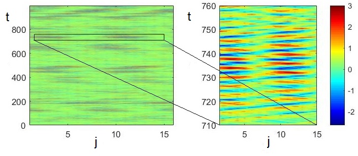
Figure 8: Color map of the displacement $q_{j}(t)$ for the system with $\epsilon=4.74$ initialized with particles at rest with initial positions as a single sine wave. A nonlinear standing wave pattern is visible.

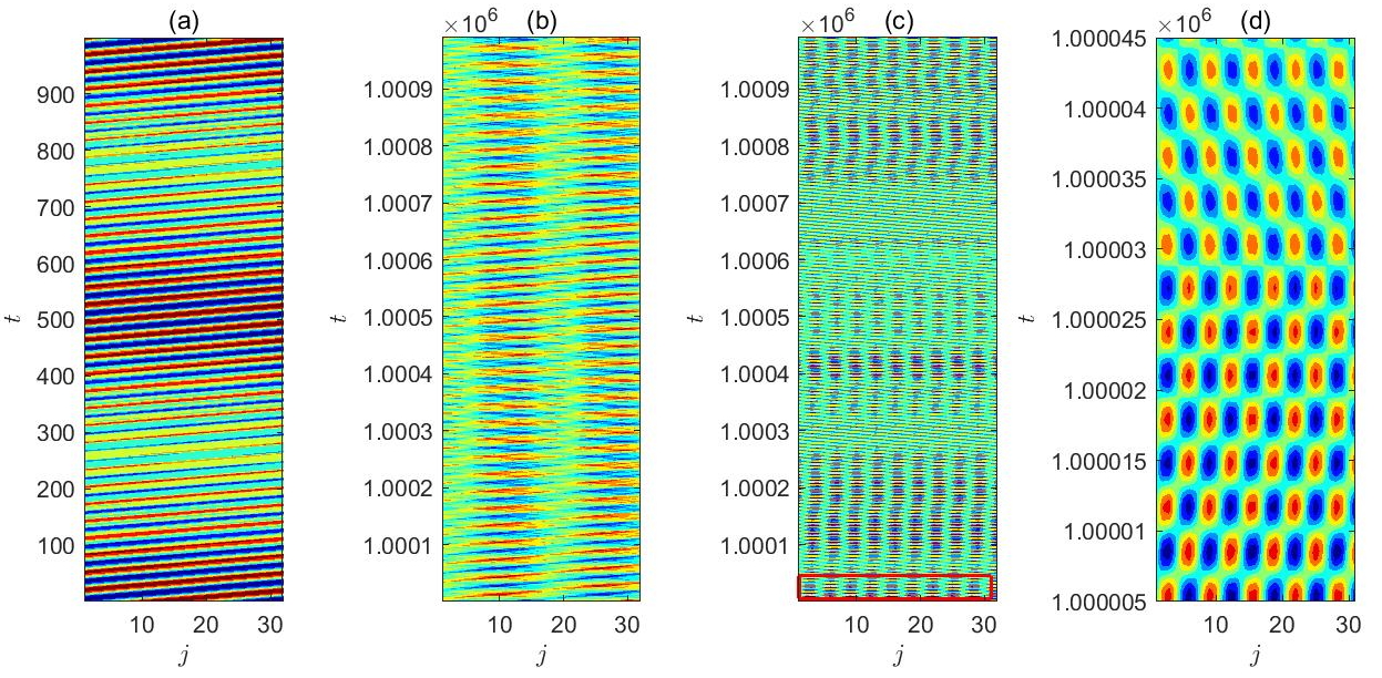
Figure 9: Color map of the displacement $q_{j}(t)$ for $\epsilon=0.02$: (a) initial traveling wave, $0<t<1000$ (b) standing wave structure in thermal equilibrium, $10^{6}<t<10^{6}+1000$ (c) $\tilde{q}_{j}(t)$, displacement after removing wave numbers $k=1...4,7...N$ (d) closer look at the boxed region in (c).

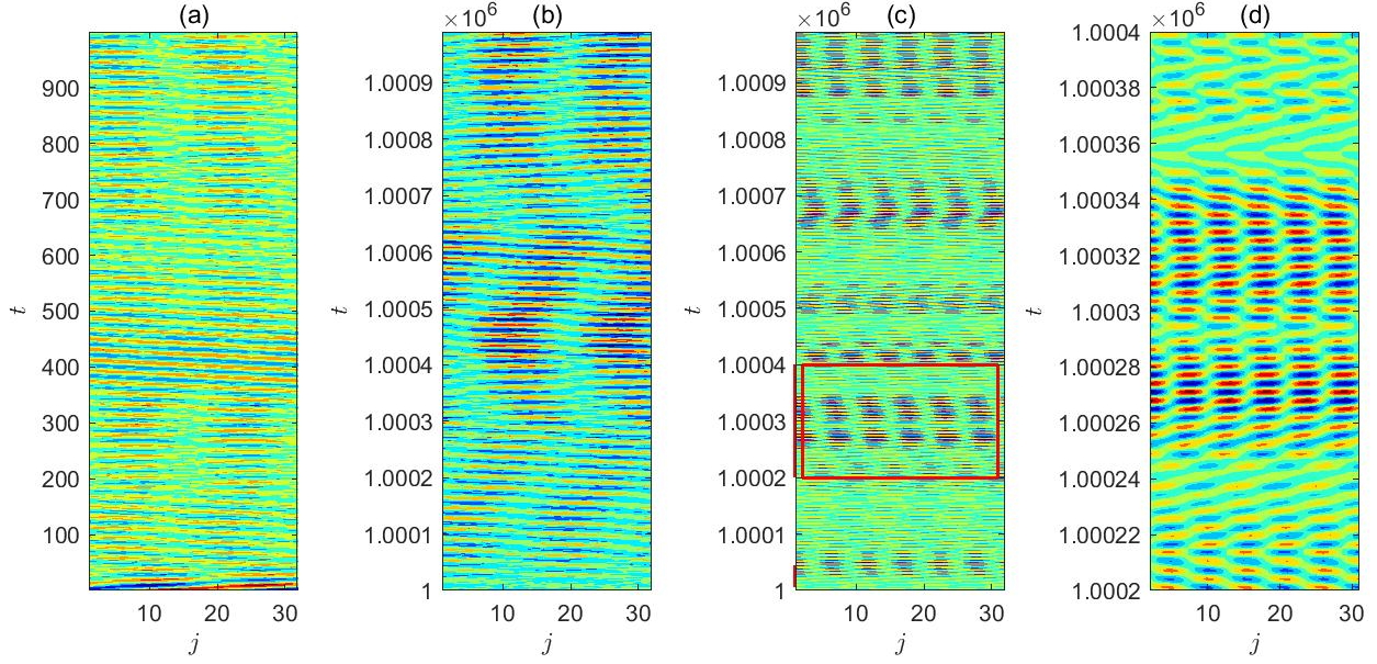
Figure 10: Color map of the displacement $q_{j}(t)$ for $\epsilon=0.54$: (a) initial traveling wave, $0<t<1000$ (b) standing wave structure in thermal equilibrium, $10^{6}<t<10^{6}+1000$ (c) $\tilde{q}_{j}(t)$, displacement after removing wave numbers $k=1...3,5...N$ (d) closer look at the boxed region in (c).

VI Conclusion

In this paper we have given the numerical evidence that anomalous correlators develop spontaneously in a classical system. From a theoretical point of view it is possible to develop a theory for weakly nonlinear dispersive waves that accounts for presence of such anomalous correlator. The framework in which the theory has been developed is the Wave Turbulence one. In such theory one usually is interested in the second order correlator $\langle a_{k_{i}}a_{k_{j}}^{*}\rangle$ which is strictly related to the wave action spectrum. However, what is clear from numerical simulations of the $\beta$-FPUT system is that also the correlator $\langle a_{k_{i}}a_{k_{j}}\rangle$ can assume values that are different from zero. This finding has consequences on the standard Wave Turbulence theory that is based on the Wick’s selection rule, i.e. the splitting of higher order correlators as a sum of products of second order correlators. Following Falkovich et al. (1992); V.S.Lvov (1994), we have generalized the Wick’s rule by including the anomalous correlators. We note that we differ from the case described in the S–theory Zakharov et al. (1975); Lvov (2012) in that there the existence of anomalous correlators was connected with coherent pumping in the system, with the anomalous correlator being a measure of partial coherence for exiting waves. In our observations and predictions, waves with random initial conditions form phase correlations with each other, resulting in an anomalous correlator which is initially zero but then saturates to a nonzero value as it evolves with time.

One of the most striking manifestation of those correlators is the appearance of “ghost excitations”, i.e. those characterized by a negative frequencies. A formula for the content of energy of such excitations as a function of the wave spectrum is obtained and compared favorably, in the weakly nonlinear, regime with numerical simulations. Moreover, we have shown that the spontaneous emergence of the anomalous correlator is strongly connected with the formation of nonlinear standing waves; indeed, the presence of those waves implies a strong correlation between the phases of positive and negative wave numbers.

Our approach paves a new road to investigate dispersive nonlinear systems by taking into account not only amplitudes of the waves, as in traditional wave turbulence, but also the phases of the waves. We conjecture that the anomalous correlators play an important role in the theory of extreme events, such as rogue waves, which form via a mechanism related to phase locking between different wave numbers Onorato et al. (2013). Phase locking also leads to the existence of solitons in nonlinear media.

As was discussed in the introduction, anomalous phase correlations have been observed to play a role in causing shifts of wave action from turbulence and condensate in the Nonlinear Schrodinger equation Bardeen (1957). Our approach of extending Wave Turbulence Theory to include the anomalous correlator could be generalized to address the role these correlations play in the statistical properties of the Nonlinear Schrodinger equation and other integrable systems. On a similar note, recurrences in an NLS-like model were shown to be directly related to the formation of anomalous phase correlations Guasoni et al. (2017); further investigating FPUT recurrences potential ties to the anomalous correlator is a subject of current work.

Finally, we emphasize that the Hamiltonian we considered is of the same family as the one for surface gravity waves (after removing by a canonical transformation nonresonant three wave interactions). We predict that also the anomalous correlators will play an important role in the understanding of statistical properties of ocean waves.

Acknowledgments The authors are grateful to Dr. B. Giulinico for discussions. We are grateful to anonymous referees, who’s insightful suggestions improved the manuscript considerably. M. O. has been funded by Progetto di Ricerca d’Ateneo CSTO160004, by the “Departments of Excellence 2018/2022” Grant awarded by the Italian Ministry of Education, University and Research (MIUR) (L.232/2016) and by Simons Foundation, Wave Turbulence. JZ and YL acknowledge support from NSF OCE grant 1635866. YL acknowledges support from ONR grant N00014-17-1-2852.

Appendix A
Matrix element in eq. (8) - The matrix elements governing four wave interactions for the variable $a_{k}(t)$ are:

$$\begin{split}&T^{(1)}_{1234}=-\frac{1}{4}\beta{\mathrm{e}^{i\pi(-k_{1}+k_{2}+k_{3}+k_{4})/N}}\prod_{i=1}^{4}\frac{2\sin(\pi k_{i}/N)}{\sqrt{\omega_{i}}},\\ &T^{(2)}_{1234}=-3T^{(1)}_{1-234},\;\;T^{(3)}_{1234}=3T^{(1)}_{4231}\;\;T^{(4)}_{1234}=-T^{(1)}_{-1234}.\end{split}$$ (30)

Matrix elements in the canonical transformation, eq. (22) - The coefficients in eq. (8) suitable for removing nonresonant terms are given by:

$$\begin{split}B^{(1)}_{1234}=\frac{T^{(1)}_{1234}}{\omega_{1}-\omega_{2}-\omega_{3}-\omega_{4}},\\ B^{(3)}_{1234}=\frac{T^{(3)}_{1234}}{\omega_{4}-\omega_{1}-\omega_{2}-\omega_{3}},\\ B^{(4)}_{1234}=\frac{T^{(4)}_{1234}}{-\omega_{1}-\omega_{2}-\omega_{3}-\omega_{4}}.\end{split}$$ (31)

Appendix B

Starting from the transformation in (22) and the generalized Wick’s decomposition in (21), we obtain:

$$\begin{split}&m_{k}^{(a)}(t)=m_{k}^{(b)}(t)+2\left(n_{k}^{(b)}(t)+n_{-k}^{(b)}(t)\right)\\ &\times\sum_{j}B^{(3)}_{k,{{-}k},j,j}n_{j}^{(b)}(t),\end{split}$$ (32)

where higher order terms in $m_{k}$ have been neglected. The next step consists in building the evolution equation for $m_{k}^{(b)}(t)$ from equation (III.1). Interestingly, the evolution equation for $m_{k}^{(b)}(t)$ appears as a deterministic dispersive non homogeneous wave evolution equation V.S.Lvov (1994),

$$\begin{split}&i\frac{dm_{k}^{(b)}}{dt}=2\tilde{\omega}_{k}m_{k}^{(b)}+\big{[}(n_{k}^{(b)}+n_{-k}^{(b)})\sum_{j}T_{k-kj-j}m_{j}^{(b)}\big{]},\end{split}$$ (33)

with $\tilde{\omega}_{k}=\omega_{k}+2\sum_{j}T_{kjkj}n_{j}^{(b))}$. Such equations have been derived in the theory of Bose Einstein condensates and superconductivity.

The equation for the spectrum, see V.S.Lvov (1994), is given by

$$\begin{split}&\frac{dn_{k}^{(b)}}{dt}=-2{\rm Im}[m_{k}^{(b)}\sum T_{k,-k,j,-j}m_{j}^{(b)*}].\end{split}$$ (34)

From equations (33) and (34), after some algebra, it is possible to show that the following interesting relations holds:

$$\begin{split}&\frac{d[|m^{(b)}(k)|^{2}]}{d{t}}=\frac{d[n_{k}^{(b)}n_{-k}^{(b)}]}{d{t}}\\ &\frac{d[n_{k}^{(b)}-n_{-k}^{(b)}]}{d{t}}=0\end{split}$$ (35)

If $n_{k}^{(b)}$ has reached energy equipartition such that $n_{k}^{(b)}=n_{-k}^{(b)}=const/\omega_{k}$ then $|m_{k}^{(b)}|=n_{k}^{(b)}$; therefore, we expect to observe equipartition also for $\omega_{k}|m_{k}^{(b)}|$.

We now consider the leading order solution of equation (33)

$$m_{k}^{(b)}(t)=m_{k}^{(b)}(t_{0})e^{-i2\tilde{\omega}_{k}t}+\text{higher order terms}.$$

and plug it in (32), and assuming that the spectrum $n_{k}$ is in stationary conditions, we get

$$\begin{split}&m_{k}^{(a)}(t)=m_{k}^{(b)}(t_{0})e^{-i2\tilde{\omega}_{k}t}+2\left(n_{k}^{(a)}(t_{0})+n_{-k}^{(a)}(t_{0})\right)\\ &\times\sum_{j}B^{(3)}_{k,{{-}k},j,j}n_{j}^{(a)}(t_{0}).\end{split}$$ (36)

Note that we have used the fact that at the leading order $n_{k}^{(b)}(t_{0})\simeq n_{k}^{(a)}(t_{0})$.
Appendix C
We consider equation eq. (22) and take the Fourier Transform in time, to get:

$$\begin{split}&a_{k_{i},\Omega_{p}}=b_{k_{i},\Omega_{p}}+\\ &+\int\sum_{j,k,l}B_{ijkl}^{(1)}b_{{j},\Omega_{q}}b_{{k},{\Omega_{r}}}b_{{l},{\Omega_{s}}}\delta_{ij}^{kl}\delta_{\Omega_{p}}^{\Omega_{q}\Omega_{r}\Omega_{s}}d\Omega_{qrs}+\\ &+\int\sum_{j,k,l}B_{ijkl}^{(3)}b_{{j},\Omega_{q}}^{*}b_{{k},{\Omega_{r}}}^{*}b_{{l},{\Omega_{s}}}\delta_{ijk}^{l}\delta_{\Omega_{p}\Omega_{q}}^{\Omega_{r}\Omega_{s}}d\Omega_{qrs}+\\ &+\int\sum_{j,k,l}B_{ijkl}^{(4)}b_{{j},\Omega_{q}}^{*}b_{{k},{\Omega_{r}}}^{*}b_{{l},{\Omega_{s}}}^{*}\delta_{ijkl}\delta_{\Omega_{p}\Omega_{q}\Omega_{r}\Omega_{s}}d\Omega_{qrs}.\end{split}$$ (37)

The next step is to build the second order correlator $\langle a(k_{i},\Omega_{l})a(k_{j},\Omega_{m})^{*}\rangle$ assuming stationarity.

We use the generalized Wick’s decomposition in (21), i.e. including the anomalous correlators. The leading order result is contained in equation (25).

References

- Falkovich et al. (1992) G. Falkovich, V. S. Lvov, and V. E. Zakharov, Kolmogorov spectra of turbulence (Springer, Berlin, 1992).
- Nazarenko (2011) S. Nazarenko, Wave turbulence, Vol. 825 (Springer, 2011).
- Benney and Newell (1969) J. Benney and A. C. Newell, “Random wave closure,” Studies in Appl. Math. 48, 1 (1969).
- Newell (1968) A. C. Newell, “The closure problem in a system of random gravity waves,” Review of Geophysics 6, 1 (1968).
- Benney and Saffmann (1966) D. J. Benney and P. Saffmann, “Nonlinear interaction of random waves in a dispersive medium,” Proc Royal. Soc 289, 301–320 (1966).
- Kadomtsev (1965) B. B. Kadomtsev, Plasma Turbulence (Academic Press, New York, 1965).
- Choi et al. (2005) Y. Choi, Y. V. Lvov, S. Nazarenko, and B. Pokorni, “Anomalous probability of large amplitudes in wave turbulence,” Physics Letters A 339, 361 (2005).
- Choi et al. (2004) Y. Choi, Y. V. Lvov, and S. Nazarenko, “Probability densities and preservation of randomness in wave turbulence,” Physics Letters A 332, 230 (2004).
- Lvov (2012) V. S. Lvov, Wave turbulence under parametric excitation: applications to magnets (Springer Science & Business Media, 2012).
- Zakharov et al. (1975) V. E. Zakharov, V. S. Lvov, and S. S. Starobinets, “Spin-wave turbulence beyond the parametric excitation threshold,” Physics-Uspekhi 17, 896–919 (1975).
- Janssen (2004) P. Janssen, The interaction of ocean waves and wind (Cambridge University Press, Cambridge, 2004) p. 379.
- Picozzi et al. (2014) A. Picozzi, J. Garnier, T. Hansson, P. Suret, S. Randoux, G. Millot, and D. N. Christodoulides, “Optical wave turbulence: Towards a unified nonequilibrium thermodynamic formulation of statistical nonlinear optics,” Physics Reports 542 (2014).
- Proment et al. (2012) D. Proment, S. Nazarenko, and M. Onorato, “Sustained turbulence in the three-dimensional grosspitaevskii model,” Physica D: Nonlinear Phenomena 241 (2012), 10.1016/j.physd.2011.06.007.
- M. Onorato and Lvov (2015) D. Proment M. Onorato, L. Vozella and Y. V. Lvov, “A route to thermalization in the -fermi-pasta-ulam system,” Proceeding of National Academy of Science 112, 4208–4213 (2015).
- V.S.Lvov (1994) V.S.Lvov, Wave Turbulence Under Parametric Excitations, Applications to Magnets (Springer-Verlag, 1994).
- Fermi et al. (1955) E. Fermi, J. Pasta, and S. Ulam, Studies of nonlinear problems, Tech. Rep. (I, Los Alamos Scientific Laboratory Report No. LA-1940, 1955).
- Pistone et al. (2018) L. Pistone, M. Onorato, and S. Chibbaro, “Thermalization in the discrete nonlinear klein-gordon chain in the wave-turbulence framework,” EPL (Europhysics Letters) 121, 44003 (2018).
- Lvov and Onorato (2018) Y. V. Lvov and M. Onorato, “Double scaling in the relaxation time in the -fermi-pasta-ulam-tsingou model,” Physical review letters 120, 144301 (2018).
- Lee et al. (2013) W. Lee, G. Kovacic, and D. Cai, “Generation of dispersion in nondispersive nonlinear waves in thermal equilibrium,” Proceedings of the National Academy of Sciences of the United States of America 110, 3237–3241 (2013).
- Zakharov (1968) V Zakharov, “Stability of period waves of finite amplitude on surface of a deep fluid,” J. Appl. Mech. Tech. Phys. 9, 190–194 (1968).
- Bustamante et al. (2019) Miguel D Bustamante, Kevin Hutchinson, Yuri V Lvov, and Miguel Onorato, “Exact discrete resonances in the fermi-pasta-ulam–tsingou system,” Communications in Nonlinear Science and Numerical Simulation 73, 437–471 (2019).
- Yoshida (1990) H. Yoshida, “Construction of higher order symplectic integrators,” Physics Letters A 150, 262–268 (1990).
- Guasoni et al. (2017) M. Guasoni, J. Garnier, B. Rumpf, D. Sugny, J. Fatome, F. Amrani, G. Millot, and A. Picozzi, “Incoherent fermi-pasta-ulam recurrences and unconstrained thermalization mediated by strong phase correlations,” Physical Review X 7, 011025 (2017).
- Krasitskii (1994) V P Krasitskii, “On reduced equations in the Hamiltonian theory of weakly nonlinear surface waves,” J. Fluid Mech. 272, 1–20 (1994).
- Onorato et al. (2013) M. Onorato, S. Residori, U. Bortolozzo, A. Montina, and F. T. Arecchi, “Rogue waves and their generating mechanisms in different physical contexts,” Physics Reports 528 (2013), 10.1016/j.physrep.2013.03.001.
- Bardeen (1957) J. Bardeen, L. N. Cooper, J. R. Schrieffer “Microscopic Theory of Superconductivity,” Physical Review 106, 162–164 (1957).
- Bardeen (1957) P. Miller, N. Vladimirova, F. Falkovich “Oscillations in a turbulence-condensate system,” Physical Review E 87, 065202 (2013).
- Bardeen (1991) S. Dyachenko, A.C. Newell, A. Pushkarev, V.E. Zakharov “Optical turbulence: weak turbulence, condensates and collapsing filaments in the nonlinear Schrodinger equation,” Physica D 57, 96–160 (1992).
- Bardeen (1957) N. Vladimirova, S. Derevyanko, F. Falkovich “Phase transitions in wave turbulence,” Physical Review E 85, 010101(R) (2012).