The time-resolved spectra of photospheric emission from a structured jet for gamma-ray bursts

Abstract

The quasi-thermal components found in many Fermi gamma-ray bursts (GRBs) imply that the photosphere emission indeed contributes to the prompt emission of many GRBs. But whether the observed spectra empirically fitted by the Band function or cutoff power law, especially the spectral and peak energy ($E_{p}$) evolutions can be explained by the photosphere emission model alone needs further discussion. In this work, we investigate in detail the time-resolved spectra and $E_{p}$ evolutions of photospheric emission from a structured jet, with an inner-constant and outer-decreasing angular Lorentz factor profile. Also, a continuous wind with a time-dependent wind luminosity has been considered. We show that the photosphere spectrum near the peak luminosity is similar to the cutoff power-law spectrum. The spectrum can have the observed average low-energy spectral index $\alpha$ $\sim-1$, and the distribution of the low-energy spectral index in our photosphere model is similar to that observed ($-2\lesssim$ $\alpha\lesssim 0$). Furthermore, the two kinds of spectral evolutions during the decay phase, separated by the width of the core ($\theta_{c}$), are consistent with the time-resolved spectral analysis results of several Fermi multi-pulse GRBs and single-pulse GRBs, respectively. Also, for this photosphere model we can reproduce the two kinds of observed $E_{p}$ evolution patterns rather well. Thus, by considering the photospheric emission from a structured jet, we reproduce the observations well for the GRBs best fitted by the cutoff power-law model for the peak-flux spectrum or the time-integrated spectrum.

1. INTRODUCTION

After decades of investigations, the radiation mechanism of gamma-ray burst (GRB) prompt emission remains unclear. Optically thin synchrotron emission caused by internal shocks (Rees & Meszaros, 1994) has been the most widely discussed model for many years, since it can naturally explain the non-thermal nature of the observed typical spectrum, which is a smoothly joint broken power law called the “Band” function (Band et al., 1993). Observationally, the typical low-energy photon index $\alpha$ of the Band function is around $-1$ (Preece et al., 2000; Nava et al., 2011; Zhang et al., 2011). However, this model is found to face several difficulties in recent years. First, many of the observed bursts have a harder low-energy slope than the death line $\alpha=-2/3$, which cannot be obtained by basic synchrotron theory (Crider et al., 1997; Preece et al., 1998; Kaneko et al., 2006; Goldstein et al., 2012). Second, the spectral width for a large fraction of GRBs is found so narrow that it cannot be explained by synchrotron radiation (Axelsson & Borgonovo, 2015; Yu et al., 2015). Third, the narrow distribution at a few hundred keV of the observed peak energies cannot be well explained. Finally, since only the relative kinetic energy between different shells in the internal shock model can be released, the radiation efficiency is rather low (Kobayashi et al., 1997; Lazzati et al., 1999; Guetta et al., 2001; Kino et al., 2004), which contradicts with the observed high efficiency of a few tens of percent (Fan & Piran, 2006; Zhang et al., 2007; Beniamini et al., 2015).

Due to these difficulties for the internal shock model, the photospheric emission model seems to be a promising scenario (e.g., Thompson, 1994; Mészáros & Rees, 2000; Rees & Mészáros, 2005; Pe’er & Ryde, 2011; Toma et al., 2011; Fan et al., 2012; Lazzati et al., 2013; Lundman et al., 2013; Ruffini et al., 2013; Deng & Zhang, 2014; Bégué & Pe’er, 2015; Gao & Zhang, 2015; Pe’er et al., 2015; Ryde et al., 2017; Acuner & Ryde, 2018; Hou et al., 2018; Meng et al., 2018; Li, 2019a). The photospheric emission is the reasonable result of the original fireball model (Goodman, 1986; Paczynski, 1986), since at the base of the outflow the optical depth is much greater than unity (e.g. Piran, 1999). As the fireball expands and becomes transparent, the internally trapped photons are eventually released at the photosphere. The photospheric emission model naturally explains the clustering of the peak energies and the high radiation efficiency observed.

Indeed, a quasi-thermal component has been found in tens of BATSE GRBs (Ryde, 2004, 2005; Ryde & Pe’er, 2009) and some Fermi GRBs (GRB 090902B, Abdo et al. 2009, Ryde et al. 2010, Zhang 2011; GRB100724B, Guiriec et al. 2011; GRB 110721A, Axelsson et al. 2012; GRB 100507, Ghirlanda et al. 2013; GRB 101219B, Larsson et al. 2015; and the short GRB 120323A, Guiriec et al. 2013). Especially in the case of GRB 090902B, the photospheric emission dominates the observed emission. But whether the whole observed Band function or cutoff power law is of a photosphere origin remains unknown. If they are, the quasi-thermal spectrum needs to be broadened. Two different ways of broadening have been considered currently: subphotospheric dissipation (Rees & Mészáros, 2005; Giannios, 2006; Beloborodov, 2017; Vurm & Beloborodov, 2016) and geometric broadening (Pe’er, 2008; Ito et al., 2013; Lundman et al., 2013; Deng & Zhang, 2014).

Generally, photosphere is defined as a surface where the Thompson scattering optical depth $\tau$ for a photon is $\tau=1$. Consistent with Abramowicz et al. (1991), Pe’er (2008) found that the photospheric radius $R_{\text{ph}}$ is angle-dependent for a relativistic, spherically symmetric wind, $R_{\text{ph}}(\theta)\propto$ $(\theta^{2}/3+1/\Gamma^{2})$, where $\theta$ is the angle measured from the line of sight (LOS) and $\Gamma$ is the outflow bulk Lorentz factor. But in principle, the photons can be last scattered at any position $(r,\Omega)$ inside the outflow, where $r$ is the distance from the explosion center and $\Omega(\theta,\phi)$ is the angular coordinates. Thus, a probability function $P(r,\Omega)$ is brought in to describe the possibility of last scattering at any location (Pe’er, 2008; Beloborodov, 2011; Pe’er & Ryde, 2011). Also, the observed spectrum is a superposition of a collection of blackbodies with different temperature, therefore it is broadened (namely geometric broadening).

Based on the geometric broadening, Deng & Zhang (2014) performed a detailed study of the photosphere emission spectrum for the spherically symmetric wind. They showed that the spectrum below $E_{p}$ can be modified to $F_{\nu}\sim\nu^{1.5}$ ($\alpha\sim+0.5$), which is not consistent well with the observation ($\alpha\sim-1.0$). Also, for the $E_{p}$ evolution as a function of photosphere luminosity, the $L_{\text{ph}}-E_{p}$ anti-correlation is clearly shown. The observed hard-to-soft evolution and $E_{p}$-intensity tracking (Ford et al., 1995; Liang & Kargatis, 1996; Ghirlanda et al., 2010; Lu et al., 2010, 2012) cannot be reproduced well. They thus claimed that a more complicated photosphere model may be needed. Here in this work, by considering the photosphere emission for a jet with lateral structure, we show that the observed typical low-energy photon index ($\alpha\sim-1.0$) and $E_{p}$ evolutions (hard-to-soft evolution or $E_{p}$-intensity tracking) can be obtained. Indeed within the collapsar model (MacFadyen & Woosley, 1999), as the jet gets through the collapsing progenitor star, the pressure of the surrounding gas collimates it (e.g., Zhang,Woosley & MacFadyen, 2003; Morsony, Lazzati & Begelman, 2007; Mizuta, Nagataki & Aoi, 2011), thus the jet may have angular profiles of energy flux and Lorentz factor, namely a structured jet (e.g., Dai & Gou, 2001; Rossi et al., 2002; Zhang & Mészáros, 2002; Zhang et al., 2004; Beniamini et al., 2019; Beniamini & Nakar, 2019). Noteworthily, this structured jet is well believed to exist in GRB 170817A (the first joint detection of short GRB and gravitational wave, Lazzati et al. 2018; Lyman et al. 2018; Meng et al. 2018; Mooley et al. 2018; Zhang et al. 2018b; Ghirlanda et al. 2019), whose unusual performance of the prompt emission and the afterglow has invoked hot debate (e.g., Ai et al., 2018; Geng et al., 2018b; Li et al., 2018; Lin et al., 2018; Geng et al., 2019; Lan et al., 2019; Li et al., 2019; Wang et al., 2019). Previously, Lundman et al. (2013) showed that, with the collimated and steady-state jet the photospheric spectrum can reproduce the observed average low-energy photon index $\alpha\approx-1$. But for the photospheric emission from a structured jet, the time-resolved spectra, the spectral evolutions, more reasonable energy injection of continuous wind, the effect of variable wind luminosity and the evolution of $E_{p}$ need to be further explored, which are the main contents in our work.

We calculate the time-resolved photosphere spectra from a structured jet for progressively more reasonable energy injections: impulsive injection, continuous wind with a constant wind luminosity and continuous wind with a variable wind luminosity. We also perform the time-resolved spectral analysis of several GRBs observed by Fermi GBM and possessing a pulse that has a rather good profile, and then compare the spectral evolutions of this analysis and the model. In addition, we discuss the luminosity profiles and $E_{p}$ evolution based on the model calculation. We show that the photosphere spectrum around the peak luminosity is close to the spectrum of the cutoff power-law model, which is the best-fit model for large amounts of the time-resolved spectra in GRBs (e.g., Kaneko et al., 2006; Yu et al., 2016). Also, the spectrum can get a flattened shape ($\alpha$ $\sim-1$) below the peak, and the distribution of the low-energy spectral index is similar to that observed ($-2\lesssim$ $\alpha\lesssim 0$). Based on the model calculation, the two types of spectral evolutions (decided by the width of the core) during the decay phase are consistent with the time-resolved spectral analysis results of several Fermi multi-pulse GRBs and single-pulse GRBs, respectively. Finally, for this photosphere model we can reproduce the two types of observed $E_{p}$ evolution patterns rather well.

The paper is organized as follows. In Section 2, we describe the basic assumptions in our photosphere model. We then present the calculations of the time-resolved photosphere spectra for progressively more reasonable energy injections, the time-resolved spectral analysis of several Fermi GRBs and the discussion on $E_{p}$ evolution in Section 3. The conclusions are drawn in Section 4.

2. Basic Assumptions

Figure 1.— Basic picture of our model. Long-lasting central engine with a variable wind luminosity and an inner constant and outer decreased angular Lorentz factor profile are assumed. Different colors of the layers represent different wind luminosity (the maximum for the red, the minimum for the blue). Also, the grayscale in the lateral directions shows the Lorentz factor profile (darker for larger Lorentz factor).

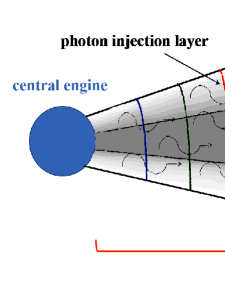
The basic physical picture of our paper is shown in Figure 1. The photons are continuously emitted into a series of layers released by a long-lasting central engine, and the wind luminosity of the central engine is time-dependent, similar to those in Deng & Zhang (2014) (see Figure 1 therein). But in our model, the jet is structured, with an inner-constant and outer-decreasing angular Lorentz factor profile (as seen in Figure 1 of Lundman et al. 2013) and an angle-independent luminosity. The angular Lorentz factor profile takes the form

$$(\Gamma-\Gamma_{\min})^{2}=\frac{(\Gamma_{0}-\Gamma_{\min})^{2}}{(\theta/\theta_{c})^{2p}+1},$$ (1)

where $\Gamma_{0}$ is the constant Lorentz factor in the jet core, $\theta_{c}$ is the half-opening angle for the jet core, $p$ is the power-law index of the profile, and $\Gamma_{\min}=1.2$ is the minimum value of the Lorentz factor.

Also, the effect of the non-zero viewing angle $(\theta_{\text{v}})$ is the same as that shown in Figure 2 of Lundman et al. (2013). There are two sets of spherical coordinates in the jet: the spherical coordinates $(r,\theta,\phi)$ with the polar axis parallel to the jet axis of symmetry and the spherical coordinates $(r,\theta_{\text{LOS}},\phi_{\text{LOS}})$ with the polar axis parallel to the LOS. The radial coordinate $(r)$ is along the axis at an angle $\theta_{\text{LOS}}$ to the LOS and $\theta$ to the jet axis.

3. THE TIME-RESOLVED SPECTRA OF MODEL AND OBSERVATION

In this section, we firstly present calculations of the time-resolved photosphere spectra for progressively more reasonable energy injections, impulsive injection in Section 3.1, continuous wind with a constant wind luminosity in Section 3.2, and continuous wind with a variable wind luminosity in Section 3.3. Then in Section 3.4, we compare them with the time-resolved spectral analysis results of several GRBs observed by Fermi GBM and possessing a pulse that has a rather good profile. Finally, discussions on the luminosity profiles and $E_{p}$ evolution patterns are presented in Section 3.5.

3.1. Impulsive Injection

Figure 2.— Instantaneous photosphere spectra from a structural jet with impulsive injection of energy. The Lorentz factor profile $\Gamma_{0}=400$, $\theta_{c}\Gamma_{0}=1$ and $p=1$ is used along with $\theta_{\text{v}}$ $=0$. A total outflow luminosity of $L=10^{52}$ erg s^-1 is assumed, base outflow radius $r_{0}=10^{8}$ cm, and luminosity distance $d_{\text{L}}=$ $4.85\times 10^{28}$ cm ($z=2$). Different line styles represent different observational times.   

.

Figure 3.— Time-resolved spectra for different Lorentz factor profiles or viewing angle. (a) A larger Lorentz factor gradient $p=4$, along with $\Gamma_{0}=400$, $\theta_{c}\Gamma_{0}=1$ and $\theta_{\text{v}}=0$. (b) $\ \Gamma_{0}=200$, with $\theta_{c}=1/$ $\Gamma_{0}$, $p=1$ and $\theta_{\text{v}}=0$.  (c)  A wider jet core $\theta_{c}=10/\Gamma_{0}=1/40$, with $\Gamma_{0}=400$, $p=1$ and $\theta_{\text{v}}=0$.  (d)  Gaussian jet with $\Gamma_{0}=400$, $\theta_{c}=1/400$, and $\theta_{\text{v}}=0$.  (e)  Non-zero viewing angle $\theta_{\text{v}}=1/200$, with $\Gamma_{0}=400$, $\theta_{c}=1/400$ and $p=1$. The yellow spectra in each figure represent the spectra of the corresponding time in Figure 2. While the black solid spectra in Figure 3c are for the uniform jet. Note that the line styles and the corresponding observational times within the box in Figure 3a are applied to all the figures (from 3a to 3e).

In this section, to calculate the time-resolved spectra, we modify Equation (10) in Lundman et al. (2013) which calculates the time-integrated photospheric spectrum:

$$F_{E}^{\text{ob}}(\theta_{\text{v}}) = \frac{1}{4\pi d_{\text{L}}^{2}}\iint(1+\beta)D^{2}\frac{d\dot{N}_{\gamma}}{d\Omega}\times\frac{R_{\text{dcp}}}{r^{2}}\exp\left(-\frac{R_{\text{ph}}}{r}\right)$$ (2)

$$\times\left\{E\frac{dP}{dE}\right\}d\Omega dr,$$

where both the velocity $\beta$ and the Doppler factor $D=[\Gamma(1-\beta\cos\theta_{\text{LOS}})]^{-1}$ depend on the angle $\theta$ to the jet axis of symmetry [$\beta=\beta(\theta)$, $D=D(\theta,\theta_{\text{LOS}})$]. $\theta_{\text{LOS}}$ is the angle to the LOS. While the viewing angle $\theta_{\text{v}}$ is the angle of the jet axis of symmetry to the LOS. If $\theta_{\text{v}}=0$, then $\theta=\theta_{\text{LOS}}$. Else if  $\theta_{\text{v}}>0$, we have

$$\theta =\theta(\theta_{\text{LOS}},\phi_{\text{LOS}})$$

$$=\arccos[\cos(\theta_{\text{LOS}})\cos(\theta_{\text{v}})+\sin(\theta_{\text{LOS}})\sin(\theta_{\text{v}})\cos\phi_{\text{LOS}}].\text{ \ \ \ \ \ \ \ \ }$$ (3)

Thus, $\beta(\theta_{\text{LOS}},\phi_{\text{LOS}})=\beta[\theta(\theta_{\text{LOS}},\phi_{\text{LOS}})]$ and $D(\theta_{\text{LOS}},\phi_{\text{LOS}})=D[\theta(\theta_{\text{LOS}},\phi_{\text{LOS}}),$ $\theta_{\text{LOS}}]$.

Since the outflow luminosity is assumed to be angle-independent, the photon emission rate at the base of the outflow, $r=r_{0}$, is also independent of angle, $d\dot{N}_{\gamma}/d\Omega=\dot{N}_{\gamma}/4\pi$ and $\dot{N}_{\gamma}=L/2.7k_{\text{B}}T_{0}$, where $L$ is the total outflow luminosity and $T_{0}=(L/4\pi r_{0}^{2}ac)^{1/4}$ is the base outflow temperature.

The decoupling radius,$\ R_{\text{dcp}}$, is defined as the radius where the optical depth to scattering a photon moving in the radial direction becomes unity. While the photospheric radius, $R_{\text{ph}}$, is the radius where the optical depth to scattering a photon moving towards the observer becomes unity. Their difference is the direction where the photon propagates.

The decoupling radius,$\ R_{\text{dcp}}$, can be calculated by

$$R_{\text{dcp}}=\frac{1}{(1+\beta)\beta\Gamma^{2}}\frac{\sigma_{\text{T}}}{m_{\text{p}}c}\frac{d\dot{M}}{d\Omega},$$ (4)

where $d\dot{M}(\theta)/d\Omega=L/4\pi c^{2}\Gamma(\theta)$ is the angle-dependent mass outflow rate per solid angle. Thus, the  decoupling radius is also angle-dependent.

While the photospheric radius, $R_{\text{ph}}$, can be written as

$$R_{\text{ph}}=\frac{\sigma_{\text{T}}}{m_{\text{p}}c\sin\theta_{\text{LOS}}}\int\nolimits_{0}^{\theta_{\text{LOS}}}\frac{(1-\beta\cos\tilde{\theta}_{{}_{\text{LOS}}})}{\beta}\frac{d\dot{M}}{d\Omega}\text{ }d\tilde{\theta}_{{}_{\text{LOS}}}.\text{ \ \ \ \ \ \ \ \ \ \ \ \ \ }$$ (5)

In the former term of Equation $(\ref{a})$, $[(1+\beta)D^{2}/4\pi]\cdot(R_{\text{dcp}}/r^{2})\exp\left(-R_{\text{ph}}/r\right)$ represents the probability density function for the final scattering to happen at the radius $r$ and the angular coordinate $\Omega(\theta,\phi)$, namely, $P(r,\Omega)$. Also, this term is very similar to the probability density function used in Pe’er & Ryde (2011) and that introduced in Beloborodov (2011).

For the latter term $E\cdot(dP/dE)$, $dP/dE$ describes the probability for a photon to have an observer frame energy between $E$ and $E+$ $dE$ within volume element $dV$. It is derived as

$$\frac{dP}{dE}=\frac{1}{2.40(k_{\text{B}}T^{\text{ob}})^{3}}\frac{E^{2}}{\exp(E/k_{\text{B}}T^{\text{ob}})-1},$$ (6)

where $T^{\text{ob}}(r,\Omega)=D(\Omega)\cdot$ $T^{{}^{\prime}}(r,\Omega)$ is the observer frame temperature, $T^{{}^{\prime}}(r,\Omega)$ is the comoving temperature. Notice that the comoving temperature also depends on the angle, since the Lorentz factor $\Gamma$, the saturation radius $R_{s}$ and the photospheric radius $R_{\text{ph}}$ are all angle-dependent, i.e.,

$$T^{\prime}(r,\Omega)=\left\{\begin{array}[]{c}\frac{T_{0}}{\Gamma(\Omega)},\text{ \ \ \ \ \ \ \ \ \ \ \ \ \ \ \ \ \ \ \ }r<R_{s}(\Omega)<R_{\text{ph}}(\Omega),\\ \frac{T_{0}[r/R_{s}(\Omega)]^{-2/3}}{\Gamma(\Omega)},\text{ \ \ \ \ \ \ \ }R_{s}(\Omega)<r<R_{\text{ph}}(\Omega),\\ \frac{T_{0}[R_{\text{ph}}(\Omega)/R_{s}(\Omega)]^{-2/3}}{\Gamma(\Omega)},\text{ }R_{s}(\Omega)<R_{\text{ph}}(\Omega)<r.\end{array}\right.$$ (7)

Adding a $\delta$-function  $\delta(t-ru/\beta c)$ to Equation $(\ref{a})$, $u=(1-\beta\cos\theta_{\text{LOS}})$ here, we get the formula that calculates the instantaneous spectrum at the observer time $t$:

$$F_{E}^{\text{ob}}(\theta_{\text{v}},t) = \frac{1}{4\pi d_{\text{L}}^{2}}\iint(1+\beta)D^{2}\frac{d\dot{N}_{\gamma}}{d\Omega}\times\frac{R_{\text{dcp}}}{r^{2}}\exp\left(-\frac{R_{\text{ph}}}{r}\right)$$ (8)

$$\left\{E\frac{dP}{dE}\right\}\times\delta(t-\frac{ru}{\beta c})\text{ }d\Omega dr.$$

Since $\beta c/u$ is independent of $t$, we have $\delta(t-ru/\beta c)=(\beta c/u)\times\delta(r=\beta ct/u)$. Meanwhile, taking into account the effect of redshift, we have

$$F_{E^{\text{ob}}}^{\text{ob}}(\theta_{\text{v}},t)=\frac{1}{4\pi d_{\text{L}}^{2}}\int(1+\beta)D^{2}\frac{d\dot{N}_{\gamma}}{d\Omega}\times\frac{R_{\text{dcp}}}{r^{2}}\exp\left(-\frac{R_{\text{ph}}}{r}\right)$$

$$\text{ \ \ \ \ \ \ \ \ \ }\left\{E\frac{dP}{dE}\right\}\times\frac{\beta c}{u}\text{ }d\Omega\text{, \ \ \ \ }r=\frac{\beta ct}{u}\text{, }E=(1+z)E^{\text{ob}}.$$ (9)

So, through the numerical integration of Equation $(\ref{a0})$, we obtain the time-resolved spectra. The results are presented in Figs 2 and 3. We have considered a big set of the parameter space region: $\Gamma_{0}=200$, $400$; $p=1$, $4$; $\theta_{c}\Gamma_{0}=1$, $10$ and $\theta_{\text{v}}/\theta_{c}=0$, $2$. The Gaussian jet is considered, too. Also, a total outflow luminosity of $L=10^{52}$ erg s^-1 and the base outflow radius $r_{0}=10^{8}$ cm are assumed. A luminosity distance of $d_{\text{L}}=$ $4.85\times 10^{28}$ cm ($z=2$, which is the peak of the GRB formation rate according to Pescalli et al. 2016) is used for spectrum normalization and redshift effect.

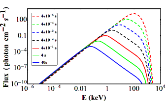
In Figure 2, we consider a narrow jet core ($\theta_{c}=1/\Gamma_{0}$) with the Lorentz factor gradient $p=1$ observed at $\theta_{\text{v}}$ $=0$. Obviously, in this case the time-resolved photosphere spectrum evolves from the pure blackbody (early on) to a power law with negative index ($F_{\nu}\sim\nu^{-1.75}$). The late-time spectrum is quite different from the flattened shape for the uniform jet (Pe’er & Ryde, 2011; Deng & Zhang, 2014). In addition, the power law has an exponential tail of blackbody emission at the high-energy end, which is the same as the case of the uniform jet.

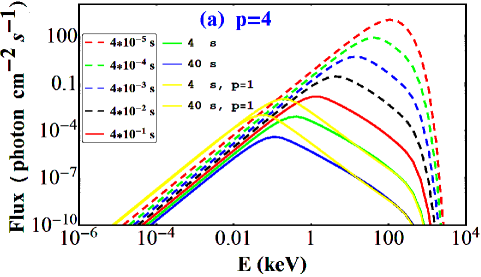
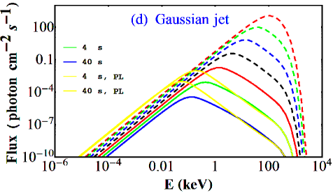
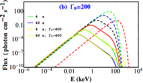
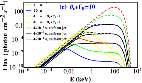
From Figure 3, we can compare the spectral evolutions for different Lorentz factor profiles or viewing angle. As shown in Figure 3a, with a larger Lorentz factor gradient $p=4$, the late-time power law is more flat. This is because that the outer jet region becomes more narrow and thus contributes less to the spectra. Also, Figure 3d is quite similar to Figure 3a, because the Lorentz factor falls down very quickly for the Gaussian profile, too. For $p=4$, when $\Gamma\sim 1$, we have $\theta\sim(\Gamma_{0}/1)^{1/4}\cdot\theta_{c}\sim 4.5\theta_{c}$; while for Gaussian jet, $\theta\sim\sqrt{2\ln(\Gamma_{0}/1)}\cdot\theta_{c}\sim 3.5\theta_{c}$. Figure 3b shows that, when $\Gamma_{0}$ is smaller the slope of the power law has no change, but the cut-off energy on the high-energy end decreases. Surely the peak energy of the early-time blackbody decreases too, and the blackbody arrives later. Furthermore, Figure 3e is close to Figure 3b, which means if the viewing angle is non-zero the spectral evolution is similar. Finally, Figure 3c presents the time-resolved spectra for a wider jet core $\theta_{c}=10/\Gamma_{0}$. Compared with the yellow spectra (for the narrow jet core), we find that the late-time power law flattens significantly, but not completely (compared with the black solid spectra for the uniform jet).

3.2. Continuous Wind with a Constant Wind Luminosity

GRBs are observed to have a duration, we thus consider the more reasonable case that the central engine produces a continuous wind. In this section, the wind luminosity and the baryon loading rate at different time are assumed to be constant, thus the Lorentz factor is also constant:

$$L_{w}(\hat{t}) = L_{0},$$

$$\dot{M}(\hat{t}) = \dot{M}_{0},$$

$$\eta(\hat{t}) = \Gamma(\hat{t})=\Gamma(\hat{t}=0),$$ (10)

where $\hat{t}$ indicates the central-engine time since the very first layer of the wind was injected.

We may consider that the wind consists of many thin layers, with each layer indicated by its injection time $\hat{t}$ . For a layer ejected from $\hat{t}$ to $\hat{t}$ $+$ $d\hat{t}$, the spectrum at the observer time $t$ (for $t>\hat{t}$) is

$$F_{E^{\text{ob}}}^{\text{ob}}(\theta_{\text{v}},t,\hat{t})=\frac{1}{4\pi d_{\text{L}}^{2}}\int(1+\beta)D^{2}\frac{d\dot{N}_{\gamma}}{d\Omega}\times\frac{R_{\text{dcp}}}{r^{2}}$$

$$\exp\left(-\frac{R_{\text{ph}}}{r}\right)\text{\ }\left\{E\frac{dP}{dE}\right\}\times\frac{\beta c}{u}\text{ }d\Omega\text{, \ \ }$$

$$r=\frac{\beta c(t-\hat{t})}{u}\text{, }E=(1+z)E^{\text{ob}}\text{.}$$ (11)

Compared with Equation $(\ref{a0})$, the only difference is  $r=\beta c(t-\hat{t})/u$. Then, by integrating over all the layers, we get the spectrum at $t$, i.e.,

$$F_{E^{\text{ob}}}^{\text{ob}}(\theta_{\text{v}},t)=\int\nolimits_{0}^{t}F_{E^{\text{ob}}}^{\text{ob}}(\theta_{\text{v}},t,\hat{t})d\hat{t}.$$ (12)

Figure 4.— Time-resolved photosphere spectra for the continuous wind with abrupt shut-down at $1$ s (red). The parameters are the same as Figure 2.

Figure 5.— Photosphere luminosity light curves of continuous winds, which shut down at $1$ s (red) and $10$ s (blue). After the shut-down, the light curves fall quickly before entering the $t^{-2}$ phase.

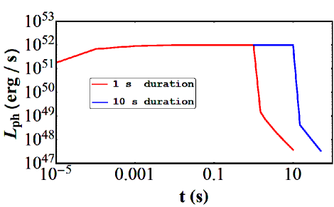
Figure 4 presents the time-resolved photosphere spectra of the continuous wind with time-independent luminosity and Lorentz factor (before $1$ s), and the spectral evolution after an abrupt shut-down (at $1$ s). Here, we take the same parameters as Figure 2. Before $1$ s, the spectrum evolves from a pure blackbody ($t=10^{-4}$ s) to the spectrum with a flattened shape ($F_{\nu}\sim\nu^{0}$) below the peak. This is caused by the superposition of emission from all layers, since the spectrum from the old layer is a power law with negative index ($F_{\nu}\sim\nu^{-1.75}$) as shown in Figure 2. The flattened shape ($F_{\nu}\sim\nu^{0}$) below the peak is consistent with the average low-energy spectral index for the time-resolved spectra observed in GRBs (e.g., Kaneko et al., 2006; Yu et al., 2016). After an abrupt shut-down (at $1$ s) the power law with negative index shows up quickly, but the flux is predominantly low, meaning that there is a rapid falling phase (see the photosphere luminosity light curves in Figure 5). This is the same as the case of the uniform jet.

3.3. Continuous Wind with a Variable Wind Luminosity

Figure 6.— Time-resolved spectra of winds with variable luminosity for different luminosity histories. A peak time $\hat{t}_{p}=2.4$ s and a peak luminosity $L_{w,\text{ }p}$ $=10^{52}$ erg s^-1 are adopted for all cases.  (a) The broken power law model with $a_{r}=0.75$ and $a_{d}=$ $-5$.  (b) The broken power law model with $a_{r}=0.75$ and $a_{d}=$ $-8$.  (c)  The exponential model with $\tau_{1}=32$, $\ \tau_{2}$ $=0.5\ \$and$\ \ \hat{t}_{s}=$ $-1.6$. The other parameters are the same as Figure 2. The Lorentz factor profile $\Gamma_{0}=400$, $\theta_{c}\Gamma_{0}=1$ and $p=1$ is used along with $\theta_{\text{v}}=0$. The base outflow radius $r_{0}=10^{8}$ cm is assumed, and luminosity distance $d_{\text{L}}=$ $4.85\times 10^{28}$ cm ($z=2$). Different colors represent different observational times.

Figure 7.— Time-resolved spectra of winds with variable luminosity for different Lorentz factor profiles.  (a) $p=4$.  (b) $\ \theta_{c}\Gamma_{0}=10$, $p=4$.  (c) $\ \theta_{c}\Gamma_{0}=10$, $p=1$.  (d) $\ \theta_{c}\Gamma_{0}=1/10$, $p=0.5$. The other parameters are the same as Figure 6c. Different colors represent different observational times.

Figure 8.— Time-resolved spectra of winds with variable luminosity for non-zero viewing angle or smaller $\Gamma_{0}$.  (a) $\ \theta_{\text{v}}$ $=1/400$.  (b) $\Gamma_{0}=200$, $\theta_{c}=1/200$.  (c) $\ \theta_{c}=1/40$, $p=4$ and $\theta_{\text{v}}$ $=1/40$. The other parameters are the same as Figure 6c. Different colors represent different observational times.

Figure 9.— Time-resolved spectra of winds with variable luminosity for different $r_{0}$ or $L_{w,\text{ }p}$.  (a) $\ r_{0}=10^{9}$ cm.  (b) $\ L_{w,\text{ }p}$ $=10^{53}$ erg s^-1. The other parameters are the same as Figure 6c. Different colors represent different observational times.

Since the light curves of the GRBs show relatively slow change in luminosity, unlike the steep rise and fall (almost within $10^{-4}$ s) for the case of constant wind luminosity, the wind luminosity may vary with time, rising and then falling gradually.

3.3.1 Wind Luminosity History

Generally, GRB pulses can be fitted well with the exponential model (Norris et al., 2005) or the smoothly joint broken power law model (Kocevski et al., 2003). So, we approximate the wind luminosity history with the broken power law model and the exponential model, respectively.

For the broken power law model, the rising and decaying indices are $a_{r}$ and $a_{d}$ respectively, along with a peak luminosity $L_{w,p}$ at $\hat{t}_{p}$. Then in the rising phase ($\hat{t}$ $<$ $\hat{t}_{p}$), the luminosity history can be written as

$$\log L_{w}(\hat{t})=a_{r}\log\hat{t}+b_{r}\text{,}$$ (13)

while in the decaying phase ($\hat{t}$ $>$ $\hat{t}_{p}$), as

$$\log L_{w}(\hat{t})=a_{d}\log\hat{t}+b_{d}\text{,}$$ (14)

where $b_{r}=\log L_{w,p}-a_{r}\log\hat{t}_{p}$ and $b_{d}=\log L_{w,p}-a_{d}\log\hat{t}_{p}$ are normalization parameters.

For the exponential model, the luminosity history can be

$$L_{w}(\hat{t} > \hat{t}_{s})=L_{w,p}\times\exp\left[2\left(\tau_{1}/\tau_{2}\right)^{1/2}\right]$$ (15)

$$\text{ \ \ \ \ \ \ \ \ }\times\exp\left(-\frac{\tau_{1}}{\hat{t}-\hat{t}_{s}}-\frac{\hat{t}-\hat{t}_{s}}{\tau_{2}}\right)\text{,}$$

where $\hat{t}_{s}$ is the start time, $\tau_{1}$ and $\tau_{2}$ are respectively the characteristic time scales indicating the rise and decay periods, $L_{w,p}$ is still the peak of luminosity at $\hat{t}_{p}$, and $\hat{t}_{p}=\hat{t}_{s}+\left(\tau_{1}\cdot\tau_{2}\right)^{1/2}$.

3.3.2 Spectra Calculation

From Equation $(\ref{a1})$, we have $R_{\text{dcp}}\propto$ $L_{w}$. In addition, $R_{s}=\Gamma r_{0}$ is independent of $L_{w}$. So we normally have $R_{\text{dcp}}\geq R_{s}$ for a relatively large $L_{w}$ ($L_{w}=10^{52}$ erg s^-1); but as the wind luminosity may rise and then fall, we may have $R_{\text{dcp}}<R_{s}$ in the relatively early and late periods of the pulse. In the following, we deal with these two cases, respectively.

$\ \ \ R_{\text{dcp}}\geq R_{s}$ Case

Since the outflow luminosity varies with time, $d\dot{N}_{\gamma}/d\Omega$ is surely time-dependent,

$$\frac{d\dot{N}_{\gamma}(\hat{t})}{d\Omega}=\frac{\dot{N}_{\gamma}(\hat{t})}{4\pi},$$

$$\dot{N}_{\gamma}(\hat{t})=\frac{L_{w}(\hat{t})}{2.7k_{\text{B}}T_{0}(\hat{t})}\text{, \ }T_{0}(\hat{t})=\left(\frac{L_{w}(\hat{t})}{4\pi r_{0}^{2}ac}\right)^{1/4}.$$ (16)

Note that $T_{0}$ is time-dependent, too.

When calculating the decoupling radius$\ R_{\text{dcp}}$,  the optical depth can be written as

$$\tau=\frac{1}{(1+\beta)\beta\Gamma^{2}}\frac{\sigma_{\text{T}}}{m_{\text{p}}c}\int\nolimits_{R_{\text{dcp}}}^{\infty}\frac{d\dot{M}}{d\Omega}\frac{1}{r^{2}}dr\text{.}$$ (17)

Here, $d\dot{M}(\theta)/d\Omega$ should depend both on $\hat{t}$ and $r$ $(r>R_{\text{dcp}})$. Also, $d\dot{M}/d\Omega$ and $\Gamma$ are both angle-dependent. We omit writing angular dependences here and below for clarity. $d\dot{M}(\hat{t},R_{\text{dcp}})/d\Omega=d\dot{M}(\hat{t})/d\Omega$ $=L_{w}(\hat{t})/4\pi c^{2}\Gamma$ is the mass outflow rate at the central engine time $\hat{t}$, while

$$\frac{d\dot{M}(\hat{t},r)}{d\Omega}=\frac{L_{w}(\hat{t}-\Delta\hat{t})}{4\pi c^{2}\Gamma}$$ (18)

denotes the mass outflow rate at $\hat{t}-\Delta\hat{t}$ (much earlier than $\hat{t}$), $\Delta\hat{t}=(r-R_{\text{dcp}})/2\Gamma^{2}\beta c$. In addition, since $\tau\thicksim 1/r$, we can set the upper limit in Equation $(\ref{b1})$ as 11$R_{\text{dcp}}$. Then, for $L_{w}=10^{52}$ erg s^-1 and $\Gamma=200$, $\Delta\hat{t}$ $\mathbf{=}$ $10(R_{\text{dcp}}/2\Gamma^{2}\beta c)\thicksim$ $3\times 10^{-3}$ s $\ll 1$ s. Thus, we may consider $d\dot{M}/d\Omega$ to be independent of $r$, which means

$$R_{\text{dcp}}(\hat{t})=\frac{1}{(1+\beta)\beta\Gamma^{2}}\frac{\sigma_{\text{T}}}{m_{\text{p}}c}\frac{d\dot{M}(\hat{t})}{d\Omega}\text{.}$$ (19)

And the other way round, when the photon emitted from the layer ($\hat{t}$) catches up with the only slightly earlier layer ($\hat{t}-\Delta\hat{t}$, $\Delta\hat{t}$ $\thicksim$ $3\times 10^{-3}$ s), it has reached a quite large radius 11$R_{\text{dcp}}$. This means that the assumption of infinity outer boundary is reasonable.

For the same reason, we take $d\dot{M}(\hat{t},r)/d\Omega\simeq d\dot{M}(\hat{t},R_{\text{ph}})/d\Omega=d\dot{M}(\hat{t})/d\Omega$ $(r>R_{\text{ph}})$, regardless of the angle-dependent $\Delta\hat{t}$. Thus, the time-dependent photospheric radius $R_{\text{ph}}(\hat{t})$ can be written as

$$R_{\text{ph}}(\hat{t})=\frac{\sigma_{\text{T}}}{m_{\text{p}}c\sin\theta_{\text{LOS}}}\int\nolimits_{0}^{\theta_{\text{LOS}}}\frac{1-\beta\cos\tilde{\theta}_{{}_{\text{LOS}}}}{\beta}\frac{d\dot{M}(\hat{t})}{d\Omega}d\tilde{\theta}_{{}_{\text{LOS}}}.$$ (20)

Then, the comoving temperature $T^{{}^{\prime}}(r,\Omega,\hat{t})$ can be obtained by (omitting angular dependences):

$$T^{\prime}(r,\hat{t})=\left\{\begin{array}[]{c}T_{0}(\hat{t})/\Gamma,\text{ \ \ \ \ \ \ \ \ \ \ \ \ \ \ \ \ \ \ \ \ \ \ \ }r<R_{s}<R_{\text{ph}}(\hat{t}),\text{ }\\ T_{0}(\hat{t})[r/R_{s}]^{-2/3}/\Gamma,\text{ \ \ \ \ \ \ \ \ \ }R_{s}<r<R_{\text{ph}}(\hat{t}),\text{ }\\ \text{ }T_{0}(\hat{t})[R_{\text{ph}}(\hat{t})/R_{s}]^{-2/3}/\Gamma,\text{ \ }R_{s}<R_{\text{ph}}(\hat{t})\text{ }<r.\text{ }\end{array}\right.$$ (21)

Similar to the case of constant wind luminosity, we have

$$F_{E^{\text{ob}}}^{\text{ob}}(\theta_{\text{v}},t,\hat{t})=\frac{1}{4\pi d_{\text{L}}^{2}}\int(1+\beta)D^{2}\frac{d\dot{N}_{\gamma}(\hat{t})}{d\Omega}\times\frac{R_{\text{dcp}}(\hat{t})}{r^{2}}$$

$$\exp\left(-\frac{R_{\text{ph}}(\hat{t})}{r}\right)\left\{\frac{1}{2.40}\frac{[E/k_{\text{B}}DT^{\prime}(r,\hat{t})]^{3}}{\exp[E/k_{\text{B}}DT^{\prime}(r,\hat{t})]-1}\right\}\times\frac{\beta c}{u}d\Omega,\text{\ }$$

$$\text{\ }r=\frac{\beta c(t-\hat{t})}{u}\text{, }E=(1+z)E^{\text{ob}}\text{.}$$ (22)

Then, using Equation $(\ref{c2})$ to integrate over all the layers, we get the spectrum at $t$. Note that we must judge whether we have $R_{\text{dcp}}(\hat{t})\geq R_{s}$ for the layer ejected at $\hat{t}$; if not, we should calculate as following.

$\ \ \ R_{\text{dcp}}<R_{s}$ Case

In this condition, $d\dot{N}_{\gamma}(\hat{t})/d\Omega$ is still calculated by Equation $(\ref{d1})$. As for the decoupling radius$\ R_{\text{dcp}}$, we have

$$R_{\text{dcp}}(\hat{t})=\left[\frac{\sigma_{\text{T}}}{6m_{\text{p}}c}\frac{d\dot{M}(\hat{t})}{d\Omega}r_{0}^{2}\right]^{1/3}\text{.}$$ (23)

Meanwhile, firstly $\Gamma$ depends on both $r$ and $\theta$, thus it is hard to calculate $R_{\text{ph}}(\hat{t})$. Secondly, $R_{\text{ph}}\thicksim R_{\text{dcp}}$(see the Figure 4 in Lundman et al. 2013). Thirdly, since $R_{\text{dcp}}<R_{s}$ the observed temperature is close to $T_{0}$ if $\theta$ is not too large. While as shown in Lundman et al. (2013), for a prompt GRB spectrum the part expected to be observed is formed by the photons making their final scattering at approximately $\lesssim 5/$ $\Gamma_{0}$. For simplicity, we take

$$R_{\text{ph}}(\hat{t})=R_{\text{dcp}}(\hat{t})\text{. }$$ (24)

Besides, the comoving temperature $T^{{}^{\prime}}(r,\hat{t})$ is given by

$$T^{\prime}(r,\hat{t})=T_{0}(\hat{t})/\Gamma(\hat{t})\text{,}$$ (25)

where $\Gamma(\hat{t})=R_{\text{dcp}}(\hat{t})/r_{0}$. Then, $F_{E^{\text{ob}}}^{\text{ob}}(\theta_{\text{v}},t,\hat{t})$ is still calculated by Equation $(\ref{f})$, except that

$$\beta = \beta(\hat{t})=\{1-[\Gamma(\hat{t})]^{-2}\}^{1/2}\text{,}$$

$$D = D(\hat{t})=\frac{1}{\Gamma(\hat{t})}\frac{1}{1-\beta(\hat{t})\cos\theta_{\text{LOS}}}\text{.}$$ (26)

3.3.3 Results

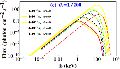
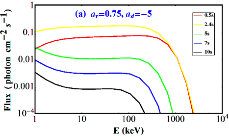
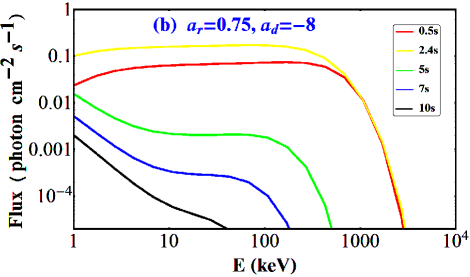
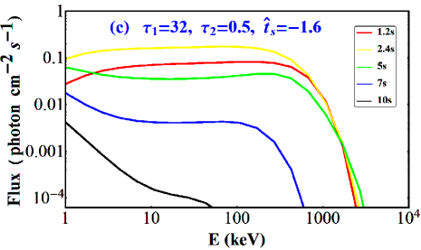
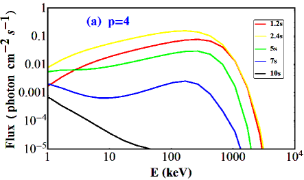
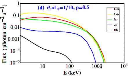
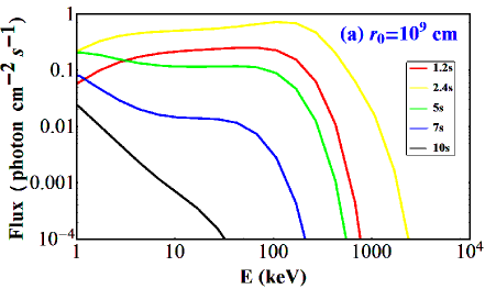
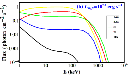
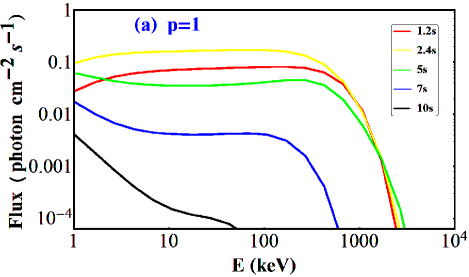
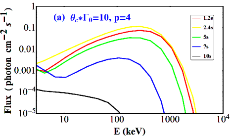
Figures 6a-6c show the calculated, instantaneous spectra of winds with variable luminosity for different luminosity histories. We fix $\hat{t}_{p}=2.4$ s, $L_{w,p}$ $=10^{52}$ erg s^-1, $r_{0}=10^{8}$ cm and $d_{\text{L}}=$ $4.85\times 10^{28}$ cm ($z=2$), and use the Lorentz factor profile $\Gamma_{0}=400$, $\theta_{c}\Gamma_{0}=1$, $p=1$ along with $\theta_{\text{v}}$ $=0$. We investigate three different luminosity profiles, the broken power law model with $(a_{r},a_{d})=(0.75,-5)$, $(0.75,-8)$ and the exponential model with $\tau_{1}=32$, $\ \tau_{2}$ $=0.5\ \$and$\ \ \hat{t}_{s}=$ $-1.6$. For each plot, different colors show different observational times. Obviously, during the rising phase ($t=0.5$ s or $1.2$ s, $2.4$ s) the resulting spectra are quite similar to those for the case of the constant luminosity (Figure 4), i.e., the spectra have a flattened shape ($F_{\nu}\sim\nu^{0}$) below the peak, consistent with the average low-energy spectral index for the time-resolved spectra observed in GRBs (e.g., Kaneko et al., 2006; Yu et al., 2016), and caused by the superposition of emission from the layers injected at different times. During the decay phase ($t=5$ s, $7$ s, $10$ s), the power law with negative index shows up gradually. The reason is that the high-latitude emission becomes more dominant (see Figure 2), since it comes from the much earlier layers that have higher luminosities. The steeper the decay phase gets, the more significant the power law with negative index is. For the broken power law model with $(a_{r},a_{d})=(0.75,-8)$ and the exponential model, the spectrum at $t=10$ s is fully a power law with negative index.

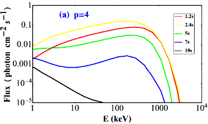
In Figures 7a-7d, we compare the resulting time-resolved spectra for different Lorentz factor profiles. The other parameters are the same as Figure 6c. As shown in Figure 7a, with a larger Lorentz factor gradient $p=4$, the resulting spectra during the rising phase ($t=$ $1.2$ s, $2.4$ s) are a little harder ($F_{\nu}\sim\nu^{0.5}$) below the peak, during the decay phase ($t=5$ s, $7$ s, $10$ s), a power law with negative index still shows up gradually. At $t=7$ s, the spectrum is the mix of a power law with negative index on the low-energy end and a modified blackbody with a shallower low-energy spectral index  ($\alpha\sim-0.5$) on the high-energy end. While the spectrum at $t=10$ s is fully a power law with negative index. Figure 7b presents the time-resolved spectra for a wider jet core with $\theta_{c}\Gamma_{0}=10$ and $p=4$, the resulting spectra during the rising phase are similar to Figure 7a, with $F_{\nu}\sim\nu^{1.0}$ below the peak. At $t=7$ s, the spectrum is still the mix of a power law with negative index and a modified blackbody with a shallower low-energy spectral index  ($\alpha\sim 0.0$). However, the spectrum at $t=10$ s is not a power law with negative index, but a modified blackbody with a flattened shape ($F_{\nu}\sim\nu^{0}$) below the peak. Figure 7c shows that, with $\theta_{c}\Gamma_{0}=10$ and $p=1$, the resulting spectra during the rising phase and the decay phase are almost the same, i.e., a modified blackbody with a shallower low-energy spectral index ($\alpha\sim 0.0$). Finally, Figure 7d presents the time-resolved spectra for a narrower jet core with $\theta_{c}\Gamma_{0}=1/10$ and $p=0.5$, the resulting spectra during the rising phase are much softer ($F_{\nu}\sim\nu^{-0.8}$) below the peak, which is consistent with the lowest low-energy spectral index for the time-resolved spectra observed in GRBs (e.g., Kaneko et al., 2006; Yu et al., 2016). During the decay phase, a power law with negative index shows up gradually also.

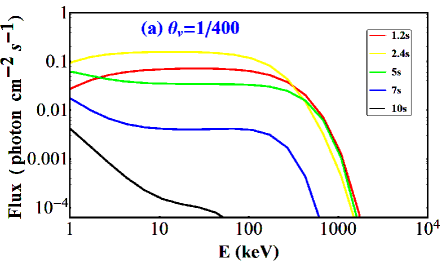
Figures 8a-8c show the resulting time-resolved spectra for non-zero viewing angle or smaller $\Gamma_{0}$. Figure 8a shows that, for a non-zero viewing angle $\theta_{\text{v}}$ $=1/400$, the resulting spectra during the rising phase are similar to those for $\theta_{\text{v}}$ $=0$ (see Figure 6c), i.e., the spectra have a flattened shape ($F_{\nu}\sim\nu^{0}$) below the peak, but the $E_{p}$ is much smaller. During the decay phase, the resulting spectra are similar to those for $\theta_{\text{v}}$ $=0$, too. For $\Gamma_{0}=200$ (smaller), $\theta_{c}=1/200$ in Figure 8b and $\theta_{c}=1/40$, $p=4$, $\theta_{\text{v}}$ $=1/40$ in Figure 8c, the resulting spectra during the rising and decay phases are similar to Figure 8a.

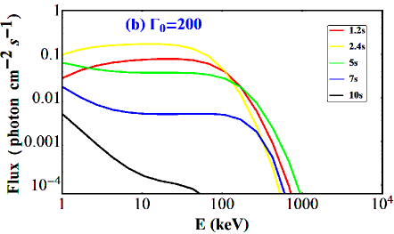
In Figures 9a and 9b, we consider the influence of different $r_{0}$ or $L_{w,p}$ on the time-resolved spectra, respectively. For$\ r_{0}=10^{9}$ cm and$\ L_{w,p}$ $=10^{53}$ erg s^-1, the resulting spectra during the rising phase change little (compared with Figure 6c). But during the decay phase, the power law with negative index shows up more quickly for $\ r_{0}=10^{9}$ cm, while same with Figure 6c for $L_{w,p}$ $=10^{53}$ erg s^-1.

3.4. Time-resolved spectral analysis of GRBs observed by Fermi GBM

Figure 10.— Comparison of the calculated time-resolved spectra for $\theta_{c}\Gamma_{0}=1$, $p=4$ and the time-resolved spectral analysis results of GRB 081125. Top left panel: the calculated time-resolved spectra for $\theta_{c}\Gamma_{0}=1$ and $p=4$, same as Figure 7a. Top right panel: the best-fit model spectra of the time-resolved spectra from GRB 081125 for several different time intervals. Middle and bottom panels: the spectral fits to the time-resolved spectra for $2.35-2.8$ s (middle left) and $6.3-9.6$ s (bottom right), and the observed spectra (fitted with the PL model) for $4.3-5.3$ s (middle right) and $5.3-6.3$ s (bottom left).

Figure 11.— Comparison of the calculated time-resolved spectra for $\theta_{c}\Gamma_{0}=1$, $p=1$ and the time-resolved spectral analysis results of GRB 090131B. Top left panel: the calculated time-resolved spectra for $\theta_{c}\Gamma_{0}=1$ and $p=1$, same as Figure 6c. Top right panel:  the best-fit model spectra of the time-resolved spectra from GRB 090131B for several different time intervals. Bottom panels: the spectral fits to the time-resolved spectra for $24.2-26.6$ s and $26.6-30$ s (from left to right), respectively.

Figure 12.— The time-resolved spectral analysis results of GRB 090626A. Left panel: the best-fit model spectra of the time-resolved spectra from GRB 090626A for several different time intervals. Right panel: the spectral fits to the time-resolved spectrum for $8.9-14$ s.

Figure 13.— Comparison of the calculated time-resolved spectra for $\theta_{c}\Gamma_{0}=10$, $p=4$ and the time-resolved spectral analysis results of GRB 081224. Top left panel: the calculated time-resolved spectra for $\theta_{c}\Gamma_{0}=10$ and $p=4$, same as Figure 7b. Top right panel: the best-fit model spectra of the time-resolved spectra from GRB 081224 for several different time intervals. Bottom panels: the spectral fits to the time-resolved spectra for $2.370-3.037$ s (left) and $8.019-13.930$ s (right), and the observed spectrum (fitted with the PL model) for $5.792-8.019$ s (middle).

Figure 14.— The time-resolved spectral analysis results of GRB 090809B. Top panel:  the best-fit model spectra of the time-resolved spectra from GRB 090809B for several different time intervals. Bottom panels: the spectral fits to the time-resolved spectra for $3.140-3.803$ s (left) and $8.5-11.3$ s (right), and the observed spectrum (fitted with the PL model) for $4.543-5.446$ s (middle).

Previously, we calculated the time-resolved spectra of winds with variable luminosity for a big set of the parameter space region. Here, we perform time-resolved spectral analysis of several GRBs observed by Fermi GBM and possessing a pulse that has a rather good profile. By comparison, we may know whether the photosphere model with an angular Lorentz factor profile can explain the observed spectral evolution well. We select the GRBs based on Lu et al. (2012), and divide the GRBs into two categories: multi-pulse GRBs (GRB 081125, GRB 090131B and GRB 090626A) which have multiple pulses, and single-pulse GRBs (GRB 081224, GRB 090809B and GRB 110817A) which have single pulse.

3.4.1 multi-pulse GRBs

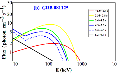
Figure 10 shows the time-resolved spectral analysis results of GRB 081125. Three different empirical models are fitted to each observed time-resolved spectrum, namely, the Band function (BAND), the cutoff power law (COMP) model and a simple power law (PL). In the top right panel, we present the model spectra of the best-fit models with corresponding parameters for $2.35-2.8$ s and $6.3-9.6$ s. The spectral fits to the time-resolved spectra for $2.35-2.8$ s and $6.3-9.6$ s are illustrated in the middle left panel and the bottom right panel, respectively. But we find that neither of the three different empirical models can fit the time-resolved spectra very well for $4.3-5.3$ s and $5.3-6.3$ s, since the time-resolved spectra seem to be fitted better with the power law model on the low-energy end and the COMP model on the high-energy end. The combined model spectra of the PL plus COMP model with corresponding rough best-fit parameters are shown in the top right panel also. The observed spectra (fitted with the PL model) for $4.3-5.3$ s and $5.3-6.3$ s are illustrated in the middle right panel and the bottom left panel, respectively. We find that the observed spectral evolution is quite similar to that for the case of $\theta_{c}\Gamma_{0}=1$ and $p=4$ (shown in the top left panel, and same as Figure 7a). The spectra during the rising phase ($t=$ $1.2$ s, $2.4$ s for model, $2.35-2.8$ s for observation) are cutoff power law with a little harder than the flattened shape below the peak, during the decay phase ($t=5$ s, $7$ s, $10$ s for model, $4.3-5.3$ s, $5.3-6.3$ s and $6.3-9.6$ s for observation), a power law with negative index shows up gradually. At $t=7$ s for model and $4.3-5.3$ s, $5.3-6.3$ s for observation, the spectra are all the mix of the power law with negative index on the low-energy end and the modified blackbody with a shallower low-energy spectral index (larger than $-1$) on the high-energy end. While the spectra at $t=10$ s for model and $6.3-9.6$ s for observation both are fully the power law with negative index. Our best-fit results of the time-resolved spectra from GRB 081125 are almost consistent with those of Yu et al. (2016), where the best-fit models before $3.615$ s are all the COMP model and the best-fit models after $3.615$ s are the PL model.

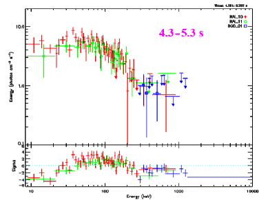
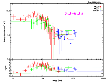
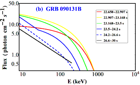
Similarly, Figure 11 shows the time-resolved spectral analysis results of GRB 090131B. The best-fit results of the time-resolved spectra for several different time intervals are presented in the top right panel. In the bottom panels, the spectral fits to the time-resolved spectra for $24.2-26.6$ s (left) and $26.6-30$ s (right) are illustrated. The observed spectral evolution is found to be quite similar to that for the case of $\theta_{c}\Gamma_{0}=1$ and $p=1$ (shown in the top left panel, and same as Figure 6c). The spectra during the rising phase ($t=$ $1.2$ s, $2.4$ s for model, $22.658-22.907$ s, $22.907-23.168$ s for observation) are cutoff power law with the flattened shape below the peak, during the decay phase ($t=5$ s, $7$ s, $10$ s for model, $23.5-24.2$ s, $24.2-26.6$ s and $26.6-30$ s for observation), a power law with negative index shows up gradually. At $t=7$ s for model and $23.5-24.2$ s for observation, the spectra both are the mix of the power law with negative index on the low-energy end and the modified blackbody with the low-energy flattened shape on the high-energy end. While the spectra at $t=10$ s for model and $24.2-26.6$ s, $26.6-30$ s for observation (see the two bottom panels) are all fully the power law with negative index. Our best-fit results of the time-resolved spectra from GRB 090131B are also almost consistent with those of Yu et al. (2016), where the best-fit models before $23.422$ s are all the COMP model and the best-fit models after $23.898$ s are the PL model.

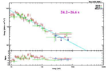
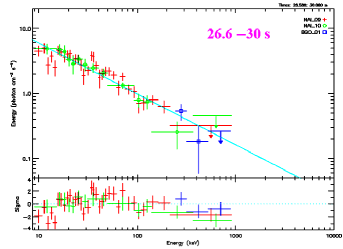
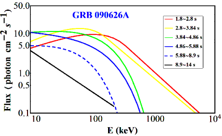
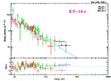
Also, Figure 12 shows the time-resolved spectral analysis results of GRB 090626A. The best-fit results of the time-resolved spectra for several different time intervals are presented in the left panel, and the spectral fits to the time-resolved spectrum for $8.9-14$ s in the right panel. The observed spectral evolution is similar to that for the case of $\theta_{c}\Gamma_{0}=1$ and $p=1$ (see Figure 6c), too. And the best-fit results of the time-resolved spectra are also almost consistent with those of Yu et al. (2016), where the best-fit models after $5.888$ s are the PL model.

3.4.2 single-pulse GRBs

Figure 15.— The time-resolved spectral analysis results of GRB 110817A. Top panel:  the best-fit model spectra of the time-resolved spectra from GRB 110817A for several different time intervals. Bottom panels: the spectral fits to the time-resolved spectra for $1.3-1.7$ s (left) and $3.7-6.3$ s (right), and the observed spectrum (fitted with the PL model) for $2.2-2.7$ s (middle).

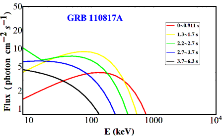
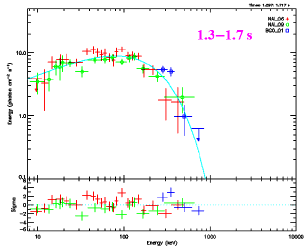
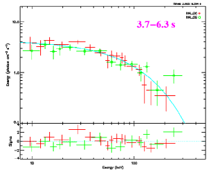
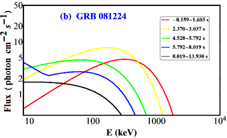
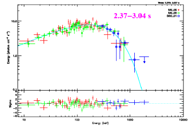
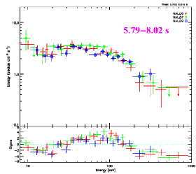
Figure 13 shows the time-resolved spectral analysis results of GRB 081224. The best-fit results of the time-resolved spectra for several different time intervals are presented in the top right panel. In the bottom panels, the spectral fits to the time-resolved spectra for $2.370-3.037$ s (left) and $8.019-13.930$ s (right), and the observed spectra (fitted with the PL model) for $5.792-8.019$ s (middle) are illustrated. The observed spectral evolution is found to be quite similar to that for the case of $\theta_{c}\Gamma_{0}=10$ and $p=4$ (shown in the top left panel, and same as Figure 7b). The spectra during the rising phase ($t=$ $1.2$ s, $2.4$ s for model, $2.370-3.037$ s for observation) are still the cutoff power law with a little harder than the flattened shape below the peak. At $t=7$ s for model and $5.792-8.019$ s for observation, the spectra both are the mix of the power law with negative index on the low-energy end and the modified blackbody with a shallower low-energy spectral index (larger than $-1$) on the high-energy end. However, the spectra at $t=10$ s for model and $8.019-13.930$ s for observation are not the power law with negative index, but the modified blackbody with the flattened shape ($F_{\nu}\sim\nu^{0}$) below the peak. The best-fit results of the time-resolved spectra are almost consistent with those of Yu et al. (2016), where the best-fit models before $13.975$ s are all the COMP model and the best-fit low-energy spectral index changes from $-0.2$ to $-1$.

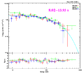
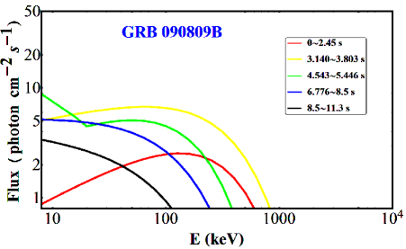
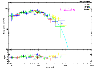
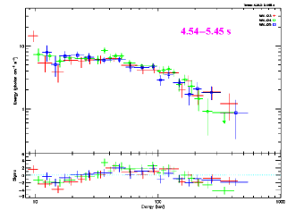
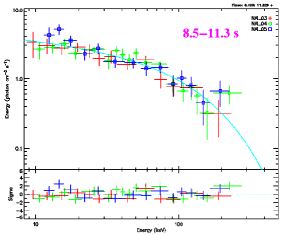
Figures 14 and 15 present the time-resolved spectral analysis results of GRB 090809B and GRB 110817A, respectively. The observed spectral evolution for each is similar to that for GRB 081224, thus the case of $\theta_{c}\Gamma_{0}=10$ and $p=4$. The best-fit results of the time-resolved spectra are also almost consistent with those of Yu et al. (2016).

According to the above analyses, we can see that the photosphere model with an angular Lorentz factor profile may explain the observed spectral evolution well. In addition, the observed spectral evolutions for multi-pulse GRBs and single-pulse GRBs seem to be different. The $\theta_{c}$ for multi-pulse GRBs seems to be more narrow, while much wider for the single-pulse GRBs.

3.5. Luminosity profiles and $E_{p}$ evolution

Figure 16.— The initial wind luminosity $L_{w}$ and photosphere luminosity $L_{\text{ph}}$ profiles. For comparison, the photosphere luminosity $L_{\text{ph}}$ profiles have all been normalized to $L_{w,\text{ }p}$ $=10^{52}$ erg s^-1 at $2.4$ s. The initial wind luminosity $L_{w}$ profiles for the exponential model ($\tau_{1}=32$, $\tau_{2}$ $=0.5$, $\hat{t}_{s}=$ $-1.6$) and the broken power law model ($a_{r}=0.75$, $a_{d}=$ $-5$) are plotted by the red solid line and the blue solid line, respectively. The photosphere luminosity $L_{\text{ph}}$ profiles for the exponential model with various parameters are shown by the points of different shapes and colors at $1.2$ s, $2.4$ s and $5$ s. While the photosphere luminosity $L_{\text{ph}}$ profile for the broken power law model with the typical parameters ($\theta_{c}\Gamma_{0}=1$, $p=1$, $\theta_{v}$ $=0$ ) is shown by the blue triangle points at $2.4$ s, $4$ s and $6$ s. The three dashed lines are the light curves for GRB 110817A (orange), GRB 081224 (black) and GRB 090131B (green), respectively.

Figure 17.— Evolution of $E_{p}$ for different parameters. Top left panel: initial wind luminosity $L_{w}$ (green dashed line) and evolution of $E_{p}$ with “$\theta_{c}\Gamma_{0}=1$, $p=1$”(red solid line), “$\theta_{c}\Gamma_{0}=10$, $p=4$”(orange solid line) or a uniform jet (black solid line) for the case “$\tau_{1}=32$, $\tau_{2}=0.5$, $\hat{t}_{s}=-1.6$”. Top right panel: $E_{p}$ evolution (red solid line), the initial wind luminosity $L_{w}$ (green dashed line) and the photosphere luminosity $L_{\text{ph}}$ (black circle points and blue solid line) for the case “$a_{r}=0.75$, $a_{d}=$ $-5$”. The $E_{p}$ is for the time-integrated spectra here, which have a time bin of $1$ $s$ (The $E_{p}$ at $1.5$ s is for the time interval of $1-2$ s, and so on).  Bottom panel: initial wind luminosity $L_{w}$ (green dashed line) and evolution of $E_{p}$ with $r_{0}=10^{9}$ cm (red solid line) for the case “$\tau_{1}=32$, $\tau_{2}=0.5$, $\hat{t}_{s}=-1.6$”.

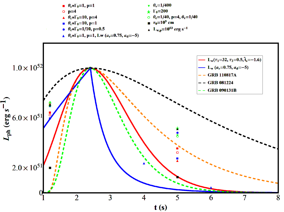
The light curve is an important observational characteristic for GRBs. Here, in Figure 16, we use the light curve profiles of a few GRBs to test the reasonability of our initial wind luminosity $L_{w}$ profiles. Also, we explore the parameter dependencies of the photosphere luminosity $L_{\text{ph}}$ profiles. For the initial wind luminosity $L_{w}$ profile of $a_{r}=0.75$ and $a_{d}=$ $-5$, the photosphere luminosity $L_{\text{ph}}$ profile (blue triangle points) is close to the light curve profile of GRB 090131B. While for the initial wind luminosity $L_{w}$ profile of $\tau_{1}=32$, $\tau_{2}$ $=0.5$ and $\hat{t}_{s}=$ $-1.6$, the photosphere luminosity $L_{\text{ph}}$ profiles (the points of different shapes and colors for various parameters) are close to the light curve profile of GRB 110817A. As for the parameter dependencies, the photosphere luminosity $L_{\text{ph}}$ falls down more rapidly for a wider jet core ($\theta_{c}\Gamma_{0}=10$, $p=1$ or $\theta_{c}\Gamma_{0}=10$, $p=4$) or larger $r_{0}$ ($r_{0}=10^{9}$ cm), and more slowly for a narrower jet core ($\theta_{c}\Gamma_{0}=1/10$, $p=0.5$), smaller $\Gamma_{0}$ ($\Gamma_{0}=200$), non-zero viewing angle ($\theta_{\text{v}}$ $=1/400$ or $\theta_{c}=1/40$, $p=4$, $\theta_{\text{v}}$ $=1/40$) or larger $L_{w,p}$ ($L_{w,p}$ $=10^{53}$ erg s^-1).

Furthermore, the evolution of $E_{p}$ is crucial to judge whether a GRB prompt emission model is better. Observationally, the hard-to-soft evolution and intensity-tracking patterns have been identified (Ford et al., 1995; Liang & Kargatis, 1996; Lu et al., 2010, 2012). For the photosphere emission model of a uniform jet, Deng & Zhang (2014) showed that the observed hard-to-soft evolution pattern cannot be reproduced, and the $E_{p}-L$ tracking pattern can be reproduced when the dimensionless entropy $\eta$ depends positively on $L_{w}$. Here, by considering the structured jet and including the $R_{\text{ph}}<R_{s}$ regime, we can reproduce the hard-to-soft evolution and intensity-tracking patterns better with the photosphere model.

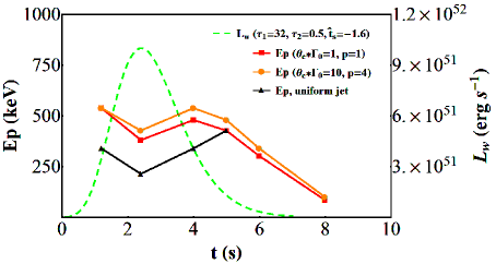
Based on the numerical results of the time-resolved spectra presented in Figure 6c ($\theta_{c}\Gamma_{0}=1$, $p=1$) and Figure 7b ($\theta_{c}\Gamma_{0}=10$, $p=4$), we plot the evolution of $E_{p}$ with respect to wind luminosity ($\tau_{1}=32$, $\tau_{2}=0.5$, $\hat{t}_{s}=-1.6$) in the top left panel of Figure 17. An approximate hard-to-soft evolution is shown, except for a slight increase after the peak of $L_{w}$. The evolution is similar for other Lorentz factor profiles and viewing angles considered above. Now, we perform some analytical discussions. For the regime $R_{\text{ph}}>R_{s}$ (relatively large $L_{w}$ near the peak), the observed temperature can be expressed as

$$T_{\text{ph}}(\theta) \propto L_{w}^{1/4}r_{0}^{-1/2}[R_{\text{ph}}(\theta)/R_{s}(\theta)]^{-2/3}$$ (27)

$$\propto L_{w}^{1/4}r_{0}^{-1/2}\{[L_{w}/\Gamma^{3}(\theta)]/[\Gamma(\theta)r_{0}]\}^{-2/3}$$

$$\propto L_{w}^{-5/12}r_{0}^{1/6}\Gamma^{8/3}(\theta).$$

Here, the observed temperature is angle-dependent. Compared with the case of a uniform jet (black solid line), the $L_{w}-E_{p}$ anti-correlation is much weaker. And if we consider the time-integrated spectra, the anti-correlation may almost disappear. Then as the $L_{w}$ falls down, one enters the regime $R_{\text{ph}}<R_{s}$, and

$$T_{\text{ph}}(\theta)\propto L_{w}^{1/4}r_{0}^{-1/2}.$$ (28)

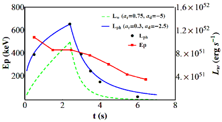
Now, we have $E_{p}\propto L_{w}^{1/4}$, which means $E_{p}$ decreases. Thus, a approximate hard-to-soft evolution shows up. For the time-integrated spectra of the wind luminosity $a_{r}=0.75$, $a_{d}=$ $-5$ which has a steeper decay phase, the hard-to-soft evolution is rather well as showed in the top right panel of Figure 17. For this wind luminosity, the photosphere luminosity $L_{\text{ph}}$ in the decay phase has an index of $a_{d}=$ $-2.5$ which is consistent with the average decay phase index $d=2.44\pm 0.12$ of a large sample of GRBs in Kocevski et al. (2003). In addition, with a larger $r_{0}$ ($r_{0}=10^{9}$ cm) the evolution of $E_{p}$ acts as the intensity-tracking pattern well, as showed in the bottom panel of Figure 17. This is because the $R_{\text{ph}}<R_{s}$ regime works for the whole wind profile (For the same reason, the intensity-tracking pattern can be obtained with smaller peak luminosity $L_{w,p}=10^{51}$ erg s^-1). And the much larger $r_{0}$ is consistent with the rather high mean value $\left\langle r_{0}\right\rangle\sim 10^{8.5}$ cm deduced in Pe’er et al. (2015).

4. CONCLUSIONS AND DISCUSSION

In this paper, we investigate the time-resolved spectra and $E_{p}$ evolutions of photospheric emission from a structured jet. To be more realistic, a continuous wind with a time-dependent wind luminosity has been considered. The following conclusions are drawn. (1) The photosphere spectrum near the peak luminosity is similar to the spectrum of the cutoff power-law model, which is the best-fit model for a large percentage of the time-resolved spectra in GRBs (e.g., Kaneko et al., 2006; Yu et al., 2016). (2) The photosphere spectrum near the peak luminosity can have a flattened shape ($F_{\nu}$ $\sim$ $\nu^{0}$) below the peak, consistent with the average low-energy spectral index ($\alpha$ $\sim-1$) for the time-resolved spectra observed in GRBs (e.g., Kaneko et al., 2006; Yu et al., 2016). Also, the distribution of the low-energy spectral index for our photosphere model is similar to that observed ($-2\lesssim$ $\alpha\lesssim 0$). For $\theta_{c}\Gamma_{0}=1/10$ and $p=0.5$, $\alpha$ $\sim-1.8$; for $\theta_{c}\Gamma_{0}=10$ and $p=4$, $\alpha$ $\sim 0$. (3) Judged by the width of the jet core, the spectral evolutions during the decay phase for our photosphere model can be mainly divided into two types. A power law with negative index gradually emerges for narrower core ($\theta_{c}\Gamma_{0}=1$), while a modified blackbody with a flattened shape ($F_{\nu}\sim\nu^{0}$) below the peak shows up for wider core ($\theta_{c}\Gamma_{0}=10$, $p=4$). Based on the time-resolved spectral analysis of several GRBs observed by Fermi GBM and possessing a pulse that has a rather good profile, we find that the above-mentioned two kinds of spectral evolutions during the decay phase do seem to exist. The spectral evolution for the multi-pulse GRBs is similar to that for narrower jet core, while the single-pulse GRBs similar to wider jet core. (4) For this photosphere model, we can reproduce the two types of observed $E_{p}$ evolution patterns rather well. For the typical parameters, we get the hard-to-soft evolution; and for a larger $r_{0}$ ($r_{0}=10^{9}$ cm) or smaller $L_{w,p}$ ($L_{w,p}=10^{51}$ erg s^-1), we have the intensity-tracking pattern. From the above, by considering the geometrical broadening for structured jet, we reproduce the observed time-resolved spectra, the spectral evolutions and $E_{p}$ evolutions well for the GRBs best fitted by the cutoff power-law model for the peak-flux spectrum or the time-integrated spectrum.

Photospheric emission for spherically symmetric outflows has been investigated by several authors (Pe’er, 2008; Beloborodov, 2011; Pe’er & Ryde, 2011; Deng & Zhang, 2014). But hydrodynamic simulations for a jet propagating through the envelope of the progenitor star (Zhang,Woosley & MacFadyen, 2003; Mizuta et al., 2006; Morsony, Lazzati & Begelman, 2007; Lazzati et al., 2009; Nagakura et al., 2011) show that the jet should have lateral structure and rapid time variability. Thus, in this paper we consider an angular Lorentz factor profile and a continuous wind with a time-dependent wind luminosity. Lundman et al. (2013) showed that, with an inner-constant and outer-decreasing angular Lorentz factor profile and steady-state jet, the photospheric spectrum can reproduce the observed average low-energy photon index $\alpha\approx-1$. But whether the time-resolved spectra, the spectral evolutions and $E_{p}$ evolutions for more reasonable energy injection of continuous wind can match the observations needs to be further considered, which have been carefully treated in this paper. And we find that they match well for the GRBs best fitted by the cutoff power-law model for the peak-flux spectrum or the time-integrated spectrum. We only give a rough comparison here since we mainly focus on the model calculations, the complete fit to the data with the model will be further explored in future works.

In this work, we assumed a local thermal radiation spectrum for each independently-evolving angular fluid element and ignored the sideway diffusion effect of photons at certain angular distance. The sideway diffusion can cause a smearing out effect on temperature and lead to a non-thermal spectrum due to inverse Compton radiation for jets with $\theta_{c}\sim 1/\Gamma_{0}$ (Ito et al 2013, Lundman et al 2013). Such effect unfortunately can not be calculated by the approach in this paper. We thus caution the spectral calculations performed in this paper when $\theta_{c}$ $\sim$ $1/\Gamma_{0}$, and especially when $\theta_{c}$ $\ll$ $1/\Gamma_{0}$.

In addition, we consider non-dissipative fireball dynamics here. The radial distributions of the Lorentz factor and the comoving temperature in dissipative outflows are significantly different (Giannios, 2012; Beloborodov, 2013). Energy dissipation in the area of moderate optical depth has been proposed by many authors, with various dissipative mechanisms such as shocks (Pe’er et al., 2005, 2006; Lazzati & Begelman, 2010), magnetic reconnection (Giannios, 2006; Giannios & Spruit, 2007; Beniamini & Giannios, 2017) and proton–neutron nuclear collisions (Beloborodov, 2010; Vurm et al., 2011). Then, relativistic electrons are generated that upscatter the thermal photons to shape the non-thermal spectrum above the peak energy. Namely, we may get the Band function spectrum with the observed low-energy photon index if the subphotospheric dissipation and the geometric broadening (for structured jet) coexist. So, decided by whether the dissipation exists, we may obtain the two kinds of spectra (COMP or Band) for the peak-flux spectrum or the time-integrated spectrum within the framework of the photosphere model.

References

- Abdo et al. (2009) Abdo, A. A., Ackermann, M., Ajello, M., et al. 2009, ApJL, 706, L138
- Abramowicz et al. (1991) Abramowicz, M. A., Novikov, I. D., & Paczynski, B. 1991, ApJ, 369, 175
- Acuner & Ryde (2018) Acuner, Z., & Ryde, F. 2018, MNRAS, 475, 1708
- Ai et al. (2018) Ai, S., Gao, H., Dai, Z.-G., et al. 2018, ApJ, 860, 57
- Axelsson et al. (2012) Axelsson, M., Baldini, L., Barbiellini, G., et al. 2012, ApJL, 757, L31
- Axelsson & Borgonovo (2015) Axelsson, M., & Borgonovo, L. 2015, MNRAS, 447, 3150
- Band et al. (1993) Band, D., Matteson, J., Ford, L., et al. 1993, ApJ, 413, 281
- Bégué & Pe’er (2015) Bégué, D., & Pe’er, A. 2015, ApJ, 802, 134
- Beloborodov (2010) Beloborodov, A. M. 2010, MNRAS, 407, 1033
- Beloborodov (2011) Beloborodov, A. M. 2011, ApJ, 737, 68
- Beloborodov (2013) Beloborodov, A. M. 2013, ApJ, 764, 157
- Beloborodov (2017) Beloborodov, A. M. 2017, ApJ, 838, 125
- Beniamini et al. (2015) Beniamini, P., Nava, L., Duran, R. B., & Piran, T. 2015, MNRAS, 454, 1073
- Beniamini & Giannios (2017) Beniamini, P., & Giannios, D. 2017, MNRAS, 468, 3202
- Beniamini & Nakar (2019) Beniamini, P., & Nakar, E. 2019, MNRAS, 482, 5430
- Beniamini et al. (2019) Beniamini, P., Petropoulou, M., Barniol Duran, R., & Giannios, D. 2019, MNRAS, 483, 840
- Crider et al. (1997) Crider, A., Liang, E. P., Smith, I. A., et al. 1997, ApJL, 479, L39
- Dai & Gou (2001) Dai, Z. G., & Gou, L. J. 2001, ApJ, 552, 72
- Deng & Zhang (2014) Deng, W., & Zhang, B. 2014, ApJ, 785, 112
- Fan & Piran (2006) Fan, Y., & Piran, T. 2006, MNRAS, 369, 197
- Fan et al. (2012) Fan, Y.-Z., Wei, D.-M., Zhang, F.-W., & Zhang, B.-B. 2012, ApJL, 755, L6
- Ford et al. (1995) Ford, L. A., Band, D. L., Matteson, J. L., et al. 1995, ApJ, 439, 307
- Gao & Zhang (2015) Gao, H., & Zhang, B. 2015, ApJ, 801, 103
- Geng et al. (2018a) Geng, J.-J., Huang, Y.-F., Wu, X.-F., Zhang, B., & Zong, H.-S. 2018a, ApJS, 234, 3
- Geng et al. (2018b) Geng, J.-J., Dai, Z.-G., Huang, Y.-F., et al. 2018b, ApJ, 856, L33
- Geng et al. (2019) Geng, J.-J., Zhang, B., Kölligan, A., Kuiper, R., & Huang, Y.-F. 2019, ApJ, 877, L40
- Ghirlanda et al. (2010) Ghirlanda, G., Nava, L., & Ghisellini, G. 2010, A&A, 511, A43
- Ghirlanda et al. (2013) Ghirlanda, G., Pescalli, A., & Ghisellini, G. 2013, MNRAS, 432, 3237
- Ghirlanda et al. (2019) Ghirlanda, G., Salafia, O. S., Paragi, Z., et al. 2019, Science, 363, 968
- Giannios (2006) Giannios, D. 2006, A&A, 457, 763
- Giannios & Spruit (2007) Giannios, D., & Spruit, H. C. 2007, A&A, 469, 1
- Giannios (2012) Giannios, D. 2012, MNRAS, 422, 3092
- Goldstein et al. (2012) Goldstein, A., Burgess, J. M., Preece, R. D., et al. 2012, ApJS, 199, 19
- Goodman (1986) Goodman, J. 1986, ApJL, 308, L47
- Guetta et al. (2001) Guetta, D., Spada, M., & Waxman, E. 2001, ApJ, 557, 399
- Guiriec et al. (2013) Guiriec, S., Daigne, F., Hascoët, R., et al. 2013, ApJ, 770, 32
- Guiriec et al. (2011) Guiriec, S., Connaughton, V., Briggs, M. S., et al. 2011, ApJL, 727, L33
- Hou et al. (2018) Hou, S.-J., Zhang, B.-B., Meng, Y.-Z., et al. 2018, ApJ, 866, 13
- Ito et al. (2013) Ito, H., Nagataki, S., Ono, M., et al. 2013, ApJ, 777, 62
- Kaneko et al. (2006) Kaneko, Y., Preece, R. D., Briggs, M. S., et al. 2006, ApJS, 166, 298
- Kino et al. (2004) Kino, M., Mizuta, A., & Yamada, S. 2004, ApJ, 611, 1021
- Kobayashi et al. (1997) Kobayashi, S., Piran, T., & Sari, R. 1997, ApJ, 490, 92
- Kocevski et al. (2003) Kocevski, D., Ryde, F., & Liang, E. 2003, ApJ, 596, 389
- Lan et al. (2019) Lan, M.-X., Geng, J.-J., Wu, X.-F., & Dai, Z.-G. 2019, ApJ, 870, 96
- Larsson et al. (2015) Larsson, J., Racusin, J. L., & Burgess, J. M. 2015, ApJL, 800, L34
- Lazzati et al. (1999) Lazzati, D., Ghisellini, G., & Celotti, A. 1999, MNRAS, 309, L13
- Lazzati et al. (2009) Lazzati, D., Morsony, B. J., & Begelman, M. C. 2009, ApJL, 700, L47
- Lazzati & Begelman (2010) Lazzati, D., & Begelman, M. C. 2010, ApJ, 725, 1137
- Lazzati et al. (2013) Lazzati, D., Morsony, B. J., Margutti, R., & Begelman, M. C. 2013, ApJ, 765, 103
- Lazzati et al. (2018) Lazzati, D., Perna, R., Morsony, B. J., et al. 2018, Physical Review Letters, 120, 241103
- Li et al. (2018) Li, B., Li, L.-B., Huang, Y.-F., et al. 2018, ApJ, 859, L3
- Li (2019b) Li, L. 2019, ApJS, 242, 16
- Li (2019a) Li, L. 2019, arXiv:1905.02340
- Li et al. (2019) Li, L.-B., Geng, J.-J., Huang, Y.-F., & Li, B. 2019, arXiv:1901.08266
- Liang & Kargatis (1996) Liang, E., & Kargatis, V. 1996, Nature, 381, 49
- Lin et al. (2018) Lin, D.-B., Liu, T., Lin, J., et al. 2018, ApJ, 856, 90
- Lu et al. (2010) Lu, R.-J., Hou, S.-J., & Liang, E.-W. 2010, ApJ, 720, 1146
- Lu et al. (2012) Lu, R.-J., Wei, J.-J., Liang, E.-W., et al. 2012, ApJ, 756, 112
- Lundman et al. (2013) Lundman, C., Pe’er, A., & Ryde, F. 2013, MNRAS, 428, 2430
- Lü et al. (2017) Lü, H.-J., Lü, J., Zhong, S.-Q., et al. 2017, ApJ, 849, 71
- Lyman et al. (2018) Lyman, J. D., Lamb, G. P., Levan, A. J., et al. 2018, Nature Astronomy, 2, 751
- MacFadyen & Woosley (1999) MacFadyen, A. I., & Woosley, S. E. 1999, ApJ, 524, 262
- Meng et al. (2018) Meng, Y.-Z., Geng, J.-J., Zhang, B.-B., et al. 2018, ApJ, 860, 72
- Mészáros & Rees (2000) Mészáros, P., & Rees, M. J. 2000, ApJ, 530, 292
- Mizuta et al. (2006) Mizuta, A., Yamasaki, T., Nagataki, S., & Mineshige, S. 2006, ApJ, 651, 960
- Mizuta, Nagataki & Aoi (2011) Mizuta, A., Nagataki, S., & Aoi, J. 2011, ApJ, 732, 26
- Mooley et al. (2018) Mooley, K. P., Deller, A. T., Gottlieb, O., et al. 2018, Nature, 561, 355
- Morsony, Lazzati & Begelman (2007) Morsony, B. J., Lazzati, D., & Begelman, M. C. 2007, ApJ, 665, 569
- Nagakura et al. (2011) Nagakura, H., Ito, H., Kiuchi, K., & Yamada, S. 2011, ApJ, 731, 80
- Nava et al. (2011) Nava, L., Ghirlanda, G., Ghisellini, G., & Celotti, A. 2011, A&A, 530, A21
- Norris et al. (2005) Norris, J. P., Bonnell, J. T., Kazanas, D., et al. 2005, ApJ, 627, 324
- Paczynski (1986) Paczynski, B. 1986, ApJL, 308, L43
- Pe’er et al. (2005) Pe’er, A., Mészáros, P., & Rees, M. J. 2005, ApJ, 635, 476
- Pe’er et al. (2006) Pe’er, A., Mészáros, P., & Rees, M. J. 2006, ApJ, 642, 995
- Pe’er (2008) Pe’er, A. 2008, ApJ, 682, 463
- Pe’er & Ryde (2011) Pe’er, A., & Ryde, F. 2011, ApJ, 732, 49
- Pe’er et al. (2015) Pe’er, A., Barlow, H., O’Mahony, S., et al. 2015, ApJ, 813, 127
- Pescalli et al. (2016) Pescalli, A., Ghirlanda, G., Salvaterra, R., et al. 2016, A&A, 587, A40
- Piran (1999) Piran, T. 1999, Phys. Rep., 314, 575
- Preece et al. (1998) Preece, R. D., Briggs, M. S., Mallozzi, R. S., et al. 1998, ApJL, 506, L23
- Preece et al. (2000) Preece, R. D., Briggs, M. S., Mallozzi, R. S., et al. 2000, ApJS, 126, 19
- Rees & Meszaros (1994) Rees, M. J., & Meszaros, P. 1994, ApJL, 430, L93
- Rees & Mészáros (2005) Rees, M. J., & Mészáros, P. 2005, ApJ, 628, 847
- Rossi et al. (2002) Rossi, E., Lazzati, D., & Rees, M. J. 2002, MNRAS, 332, 945
- Ruffini et al. (2013) Ruffini, R., Siutsou, I. A., & Vereshchagin, G. V. 2013, ApJ, 772, 11
- Ryde (2004) Ryde, F. 2004, ApJ, 614, 827
- Ryde (2005) Ryde, F. 2005, ApJL, 625, L95
- Ryde & Pe’er (2009) Ryde, F., & Pe’er, A. 2009, ApJ, 702, 1211
- Ryde et al. (2010) Ryde, F., Axelsson, M., Zhang, B. B., et al. 2010, ApJL, 709, L172
- Ryde et al. (2017) Ryde, F., Lundman, C., & Acuner, Z. 2017, MNRAS, 472, 1897
- Thompson (1994) Thompson, C. 1994, MNRAS, 270, 480
- Toma et al. (2011) Toma, K., Wu, X.-F., & Mészáros, P. 2011, MNRAS, 415, 1663
- Vurm et al. (2011) Vurm, I., Beloborodov, A. M., & Poutanen, J. 2011, ApJ, 738, 77
- Vurm & Beloborodov (2016) Vurm, I., & Beloborodov, A. M. 2016, ApJ, 831, 175
- Wang et al. (2019) Wang, Y.-Z., Shao, D.-S., Jiang, J.-L., et al. 2019, ApJ, 877, 2
- Wei et al. (2017) Wei, J.-J., Zhang, B.-B., Shao, L., Wu, X.-F., & Mészáros, P. 2017, ApJ, 834, L13
- Yu et al. (2015) Yu, H.-F., van Eerten, H. J., Greiner, J., et al. 2015, A&A, 583, A129
- Yu et al. (2016) Yu, H.-F., Preece, R. D., Greiner, J., et al. 2016, A&A, 588, A135
- Yu et al. (2018) Yu, H.-F., Dereli-Bégué, H., & Ryde, F. 2018, arXiv:1810.07313
- Zhang et al. (2011) Zhang, B.-B., Zhang, B., Liang, E.-W., et al. 2011, ApJ, 730, 141
- Zhang et al. (2018a) Zhang, B.-B., Zhang, B., Castro-Tirado, A. J., et al. 2018a, Nature Astronomy, 2, 69
- Zhang et al. (2018b) Zhang, B.-B., Zhang, B., Sun, H., et al. 2018b, Nature Communications, 9, 447
- Zhang & Mészáros (2002) Zhang, B., & Mészáros, P. 2002, ApJ, 581, 1236
- Zhang et al. (2004) Zhang, B., Dai, X., Lloyd-Ronning, N. M., & Mészáros, P. 2004, ApJL, 601, L119
- Zhang et al. (2007) Zhang, B., Liang, E., Page, K. L., et al. 2007, ApJ, 655, 989
- Zhang (2011) Zhang, B. 2011, Comptes Rendus Physique, 12, 206
- Zhang & Yan (2011) Zhang, B., & Yan, H. 2011, ApJ, 726, 90
- Zhang,Woosley & MacFadyen (2003) Zhang, W., Woosley, S. E., & MacFadyen, A. I. 2003, ApJ, 586, 356