Action-based models for dwarf spheroidal galaxies and globular clusters

Abstract

A new family of self-consistent DF-based models of stellar systems is explored. The stellar component of the models is described by a distribution function (DF) depending on the action integrals, previously used to model the Fornax dwarf spheroidal galaxy (dSph). The stellar component may cohabit with either a dark halo, also described by a DF, or with a massive central black hole. In all cases we solve for the model’s self-consistent potential. Focussing on spherically symmetric models, we show how the stellar observables vary with the anisotropy prescribed by the DF, with the dominance and nature of the dark halo, and with the mass of the black hole. We show that precise fits to the observed surface brightness profiles of four globular clusters can be obtained for a wide range of prescribed velocity anisotropies. We also obtain precise fits to the observed projected densities of four dSphs. Finally, we present a three-component model of the Scupltor dSph with distinct DFs for the red and blue horizontal branch stars and the dark matter halo.

1 Introduction

Diagnosing the dynamics of collisionless systems is central to contemporary astrophysics. The systems of interest range from clusters of galaxies, through giant elliptical galaxies and disc galaxies like the Milky Way, to Magellanic and spheroidal dwarf galaxies and star clusters. All these systems are dominated by the mass contributed by some mixture of dark-matter particles and galaxies and stars, and have relaxation times that greatly exceed their crossing times. In every case comparison with observations requires one to recognize that these particles fall into distinct classes: a cluster of galaxies contains dark-matter particles, and galaxies of several morphological types; a giant elliptical galaxy contains dark-matter particles and populations of stars with distinct chemistry; the Milky way and dwarf spheroidal galaxies (hereafter dSphs) contain dark-matter particles and populations of stars of distinct chemistry and age, and a globular cluster (hereafter GC) contains stars with radically different masses and subtly different chemistry.

Until recently, dynamical models of stellar systems have been simplified to the extent of containing only one stellar population and have represented dark matter by a simple density distribution without regard to its internal dynamics. With the advent of high-resolution kinematics for billions of stars (Gaia Collaboration et al. 2018) and spectra for millions of stars (Cui et al. 2012, Gaia Collaboration et al. 2018) it has become essential to develop multi-component models of stellar systems. In such a model each observationally distinct population is represented by a distribution function (hereafter DF) $f({\bf x},{\bf v})$ that gives the probability density for finding an object of the relevant population at the phase-space point $({\bf x},{\bf v})$. Given these DFs, one can solve for the gravitational potential $\Phi({\bf x})$ that these populations jointly generate. That done, the model predicts both the spatial distribution of each population and the population’s velocity distribution at every point.

The parameters characterising each component DF can be fitted to data in a variety of ways. If individual particles are observed, as in a dwarf spheroidal galaxy, the likelihood of the data given each model and the observational uncertainties can be computed and used to find the range of parameters that is consistent with the data (e.g. Pascale et al., 2018). If individual particles are not observationally resolved, as in distant galaxies, the model’s parameters can be constrained by comparing observed surface densities and velocity moments with the model’s precisely equivalent predictions. If the number of resolved particles is large, the cost of computing individual likelihoods may be unfeasible, forcing one to bin the data and constrain parameters as in the case of unresolved particles (e.g. Cole & Binney, 2017). Whatever the scale and completeness of the data, a rigorous and tractable method of parameter constraint is available.

Models based on a DF have been considered since the beginning of stellar dynamics (Eddington 1915, Michie 1963, King 1966). These models almost invariably take advantage of the Jeans theorem to posit that the DF depends on $({\bf x},{\bf v})$ only through constants of stellar motion. The energy $E$ is the most available such constant and until recently it invariably featured as an argument of the DF. The key to producing multi-component and non-spherical models, however, proves to be to exclude $E$ from the DF in favor of the action integrals $J_{i}$ (Binney 2010, Binney 2014). A complete set of action integrals $J_{r}$, $J_{z}$ and $J_{\phi}$ is guaranteed in any spherical potential, and numerical experiments (Binney & Spergel, 1982; Ratcliff et al., 1984) with galaxy-like potentials indicate that in realistic potentials the vast majority of orbits are quasi-periodic, which guarantees the existence of action integrals (Arnold 1978). Moreover, by torus mapping (Binney & McMillan 2016) one can closely approximate any given axisymmetric Hamiltonian with one in which all orbits are quasi-periodic. Hence it is intellectually sound to require that the DF depends only on actions.

None the less, it is practicable to take the DF to depend on actions only if their values can be computed from $({\bf x},{\bf v})$. When Binney (2010) first started experimenting with DFs $f({\bf J})$, he used the adiabatic approximation to compute actions. This approximation works well only for thin-disc stars and is inapplicable to halo stars or dark-matter particles. Fortunately a technique for the evaluation of actions soon appeared that provides good accuracy for all stars and dark-matter particles. This is the ‘Stäckel Fudge’ (Binney 2012a), which involves using for an arbitrary potential formulae that are strictly valid only for Stäckel’s separable potentials (Stäckel 1893). Recently Vasiliev (2018) has released a numerical implementation of the Stäckel Fudge that is highly optimised for speed and is complemented by efficient code for solving Poisson’s equation for the potential generated by an arbitrary axisymmetric mass distribution. Sanders & Binney (2016) extended the Stäckel Fudge to non-axisymmetric potentials that have no figure rotation.

Early applications of action-based DFs were restricted to modelling the kinematics of solar-neighborhood stars in given Galactic potentials (Binney 2010, Binney & McMillan 2011, Binney 2012b, Bovy & Rix 2013). The arrival of the Stäckel Fudge opened the way for global modelling, including imposition of the self-consistency condition. Binney (2014) generalised the isochrone model (Hénon 1960) to flattened systems, and Piffl et al. (2015) presented a model disc galaxy in which populations of stars spanning a range of ages self-consistently generate the potential jointly with a realistic population of dark-matter particles. Using models of the Fornax dSph in which the potential is self-consistently generated by stars and dark matter, Pascale et al. (2018) ruled out the possibility that the phase-space distribution of the dark matter at the centre of this dark-matter dominated system has the cuspy structure that is predicted by cosmological simulations that contain only dark matter.

Central to the art of modelling stellar systems with action-based DFs is a library of analytic functions $f({\bf J})$ that can be employed for the DFs of individual components. Binney (2010) introduced a form of the ‘quasi-isothermal’  DF, which, refined by Binney & McMillan (2011), has been extensively used to model our Galaxy’s discs. Posti et al. (2015) and Williams & Evans (2015a) introduced a family of DFs $f({\bf J})$ that yield self-consistent models that have two-power-law density profiles which, inter alia, can closely match the models of Jaffe (1983), Hernquist (1990) and Navarro et al. (1996b, NFW). Cole & Binney (2017) introduced a modification of the Posti et al. (2015) DFs that flattens the model’s central cusp into a core by making the central phase-space density finite.

To model a dSph, Pascale et al. (2018) had to introduce a DF $f({\bf J})$ that produces systems with exponential rather than power-law outer density profiles. The purpose of this paper is to explore in a general way models in which the stellar component is represented by this DF. In Section 2 we establish our notation. Section 3.1 we explore the dependence of the observable properties of single-component models on the DF’s parameters. In Section 3.2 we embed these models in a dark halo and explore the dependence of the observables on the degree of dark-matter domination. In Section 3.3 we add central massive black holes to the models. In Section  4.1 we show that the density profiles of several well observed globular clusters can be accurately fitted by the models. For each cluster we display four models that differ markedly in their kinematics. In Section 4.2 we use the new DF to fit observations of the dSphs Carina, Leo I, Sculptor, Sextans and Ursa Minor. In the case of Sculptor our model assigns distinct phase-space distributions to two populations of observationally distinguishable stars and a separate component to the dark matter halo. Section 5 concludes.

2 f(J) models with multiple components

Throughout this paper DFs are normalised to have unit integral over phase space:

$$\int\text{d}^{3}{\bf q}\,\text{d}^{3}{\bf p}\,f=1,$$ (1)

where $({\bf q},{\bf p})$ is any system of canonical coordinates. Let $f_{i}({\bf J})$ be such a DF for the $i$-th component of a composite stellar system. Sometimes we require a system’s luminosity density, at other times we require its mass density. Any such phase-space density can be obtained by multiplying $f$ by an appropriate dimensional factor $Q$; for example, to obtain the dark-matter mass density we multiply the DF of dark matter by the total dark-matter mass, and to obtain the $g$-band luminosity density of a stellar component we multiply $f_{i}$ by the component’s total $g$-band luminosity.

The real-space mass densities are

$$\rho_{i}({\bf x})=M_{i}\int\text{d}^{3}{\bf v}\,f_{i}({\bf J}).$$ (2)

The line-of-sight velocity distributions (hereafter LOSVDs) are

$$\mathcal{L}_{i}({\bf x}_{\perp},v_{||})=M_{i}\frac{\int\text{d}^{2}{\bf v}_{\perp}\text{d}x_{||}\,f_{i}({\bf J})}{\int\text{d}x_{||}\,\rho_{i}({\bf x})},$$ (3)

where $||$ and $\perp$ denote components parallel and orthogonal to the line-of-sight.

Evaluation of equations (2) and (3) requires the mapping between (${\bf x}$, ${\bf v}$) and (${\boldsymbol{\theta}}$, ${\bf J}$), which depends on the model’s gravitational potential $\Phi$, which is related to $\rho_{i}$ via the Poisson equation $\nabla^{2}\Phi=4\pi G\sum_{i=0}^{N}\rho_{i}$, with $G$ the gravitational constant. We rely on the Stäckel-Fudge as implemented in the software library ‘Action-based galaxy modelling architecture’ (AGAMA) that is described in Vasiliev (2018), where one can find an extensive analysis of the extent to which action values vary along numerically integrated orbits. The variation exceeds $\sim 2$ per cent only on orbits that have been trapped by a resonance. We use AGAMA additionally to solve for self-consistently generated potentials and to compute moments of DFs. AGAMA provides an optimized interative procedure to construct a self-consistent solution, which takes at most less than four minutes using an eight core machine (for details, see Vasiliev 2018).

3 Distribution functions for dwarf spheroidals and globular clusters

Figure 1: Reference, one-component, isotropic model ($\alpha=0.5$, $\eta=0.75$). From top to bottom, anisotropy parameter, slope of the logarithmic density, density and projected density are plotted against radius. In the bottom two panels $\widetilde{\rho}_{\rm iso}(r)\equiv\rho_{\rm iso}(r)/\rho_{\rm iso}(r_{\rm c,\star})$ and $\widetilde{\Sigma}_{\rm iso}(R)\equiv\Sigma_{\rm iso}(R)/\Sigma_{\rm iso}(r_{\rm c,\star})$, where $\rho_{\rm iso}$ and $\Sigma_{\rm iso}$ are, respectively, the density and projected density and $r_{\rm c,\star}$ is the core radius, such that $\gamma_{\star}(r_{\rm c,\star})=-\frac{1}{2}$.

Figure 2: One-component models with, from left to right, $\alpha$ = 0.5, 1, 2. Orange, blue, red and green curves refer to models with $\eta=0.35,0.75,1$ and $2$, respectively. Top: anisotropy parameter. Centre: ratio between model normalized density and normalized density of the isotropic model (Fig. 2). Bottom: same as centre row, but for surface density. In the left column we show the isotropic reference model $(\alpha,\eta)=(0.5,0.75)$ only the top panel (dashed blue curve). Distances are normalized to the core radius $r_{\rm c,\star}$. We define $\widetilde{\rho}(r)\equiv\rho(r)/\rho(r_{\rm c,\star})$ and $\widetilde{\Sigma}(R)\equiv\Sigma(R)/\Sigma(r_{\rm c,\star})$. $\widetilde{\rho}_{\rm iso}$ and $\widetilde{\Sigma}_{\rm iso}$ are the density and surface density profiles of the isotropic model (Fig.2).

Figure 3: Same as Fig. 2 but now in each column $\eta$ is fixed to $\eta=0.35,0.75$ and 2, from left to right. Blue, green, red and orange curves mark models with $\alpha=0.5,1,1.5$ and $2$, respectively. In the second column, we show the isotropic reference model ($\alpha=0.5,\eta=0.75$) only in the top panel (dashed blue curve). The definitions of $\widetilde{\rho}(r)$, $\widetilde{\Sigma}(R)$ and $r_{\rm c,\star}$ are as in Fig. 2.

Figure 4: Measures of concentration versus $\alpha$ for one-component models with $\eta=0.35,\,0.75,\,1$ and $2$. Top: $r_{\rm h}/r_{0,\star}$. Centre: $\rho_{r_{\rm c,\star}}/\rho_{0,\star}$. Bottom: $\Sigma_{r_{\rm c,\star}}/\Sigma_{0,\star}$. Orange, blue, red and green curves refer to models with $\eta=0.35,\,0.75,\,1$ and $2$, respectively. $r_{0,\star}$ is defined by equation (10), $\rho_{0,\star}\equiv M_{\star}/r_{0,\star}^{3}$, $\Sigma_{0,\star}\equiv M_{\star}/r_{0,\star}^{2}$, $\rho_{r_{\rm c,\star}}\equiv\rho(r_{\rm c,\star})$ and $\Sigma_{r_{\rm c,\star}}\equiv\Sigma(r_{\rm c,\star})$. The blue circle marks the position of the isotropic model.

We define $J_{r}$, $J_{\phi}$, and $J_{z}$ as the radial, azimuthal and vertical actions, respectively, and, following Pascale et al. (2018), use the DF

$$f_{\star}({\bf J})=f_{0}\exp\biggl{[}-\biggl{(}\frac{k({\bf J})}{J_{0,\star}}\biggr{)}^{\alpha}\biggr{]},$$ (4)

with

$$k({\bf J})\equiv J_{r}+\eta_{\phi}|J_{\phi}|+\eta_{z}J_{z}.$$ (5)

The factor

$$f_{0}=\frac{\eta_{\phi}\eta_{z}\alpha}{(2\pi J_{0,\star})^{3}\Gamma(3/\alpha)},$$ (6)

where $\Gamma$ is the gamma function, normalizes $f_{\star}({\bf J})$ (equation 1). This DF produces potentially anisotropic components with density distributions that have cores and at large radii can be truncated in an adjustable way.

We restrict to spherical models by fixing $\eta_{z}=\eta_{\phi}\equiv\eta$. In a spherical potential, $J_{\phi}$ and $J_{z}$ are related to the total angular momentum $L$ by $L\equiv|J_{\phi}|+J_{z}$, so equation (5) reduces to

$$k({\bf J})=J_{r}+\eta(|J_{\phi}|+J_{z})=J_{r}+\eta L.$$ (7)

We define the stellar core radius $r_{\rm c,\star}$ as the radius where

$$\gamma_{\star}\equiv\frac{\text{d}\ln\rho_{\star}}{\text{d}\ln r}=-{\textstyle\frac{1}{2}}.$$ (8)

We define the half-mass radius $r_{\rm h}$ to be the radius of the sphere containing half of the stellar mass, and the effective radius $R_{\rm e}$ to be the radius on the plane of the sky that contains half of the projected mass.

With $\sigma_{t}$ and $\sigma_{r}$ the velocity dispersions in the tangential and radial directions, respectively,

$$\beta\equiv 1-\frac{\sigma_{t}^{2}}{2\sigma_{r}^{2}}$$ (9)

measures the amount of velocity anisotropy. Isotropic velocity distributions correspond to $\beta=0$, tangentially biased ones to $\beta<0$ and radially biased ones to $0<\beta\leq 1$.

We briefly comment on the physical meaning of the relevant free parameters of the DF (4) when the latter is multiplied by the stellar mass $M_{\star}$.

• $J_{0,\star}$: the action scale that naturally defines the length scale

  $$r_{0,\star}=\frac{J_{0,\star}^{2}}{GM_{\star}}$$ (10)

  and the velocity scale

  $$v_{0,\star}=\frac{GM_{\star}}{J_{0,\star}}.$$ (11)

  Any pair among $M_{\star}$, $J_{0,\star}$, $r_{0,\star}$ and $v_{0,\star}$, sets the model’s physical scales and can be adjusted to match some physical property of a target system (for instance, the total mass or the central velocity dispersion).

• $\alpha$: a non-negative, dimensionless parameter that mainly regulates the model’s density profile.

• $\eta$: a non-negative, dimensionless parameter that mainly controls the radial or tangential bias velocities of the model; models sharing the parameters ($\alpha$, $\eta$) are homologous.

In the case of spherical symmetry ($\eta_{\phi}=\eta_{z}$), the DF (4) can be considered a generalization of the spherical anisotropic Michie-King DF $f(E,L)$. Dealing with actions ${\bf J}$ rather than $(E,L)$ facilitates extension to multi-component and flattened models (Binney 2014). Models generated by the DF (4) lack rotation, but the model can be set rotating without changing the density distribution by adding a DF that is odd in $J_{\phi}=L_{z}$.

3.1 Spherical one-component models

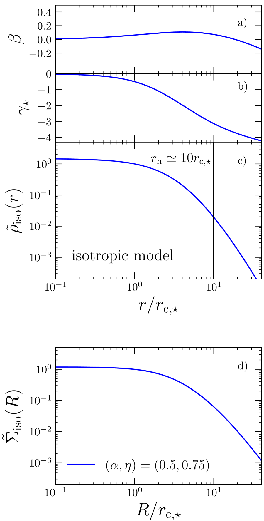
Fig. 2 plots the general properties of a nearly-isotropic model, obtained with $(\alpha,\eta)=(0.5,0.75)$. Panel a shows that the model is almost isotropic along the whole radial extent, with $|\beta|\leq 0.1$ out to $r\simeq 30r_{\rm c,\star}$. Panel c shows that the density distribution is cored, so $\gamma_{\star}\simeq 0$ near the centre, and is exponentially truncated farther out, so $\gamma_{\star}\lesssim-3$ at $r\simeq r_{\rm h}$ (panel b). The fact that an almost isotropic model is obtained when $\eta=0.75$ can be explained as follows. Since the DF $f_{\rm iso}({\bf J})$ of an isotropic model can depend on only the Hamiltonian $H$, it will satisfy

$$\frac{\partial f_{\rm iso}({\bf J})}{\partial L}\biggr{/}\frac{\partial f_{\rm iso}({\bf J})}{\partial J_{r}}=\frac{\Omega_{L}}{\Omega_{r}},$$ (12)

where $\Omega_{L}=\partial H/\partial L$ and $\Omega_{r}=\partial H/\partial J_{r}$ are, respectively, the tangential and radial frequencies. We expect $\Omega_{L}/\Omega_{r}$ to be a smooth function of ${\bf J}$, ranging from 1/2 for small actions (where $\Phi$ is almost simple-harmonic) to 1 for large actions (where $\Phi$ is almost Keplerian). However, the DF (4) is such that

$$\frac{\partial f_{\star}({\bf J})}{\partial L}\biggr{/}\frac{\partial f_{\star}({\bf J})}{\partial J_{r}}=\eta,$$ (13)

independent of the actions. The choice $\eta\simeq 0.75$ reasonably ensures a good compromise between the expected $\Omega_{L}/\Omega_{r}$ in the two regimes of small and large actions.

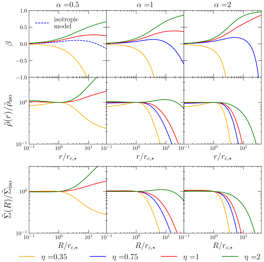
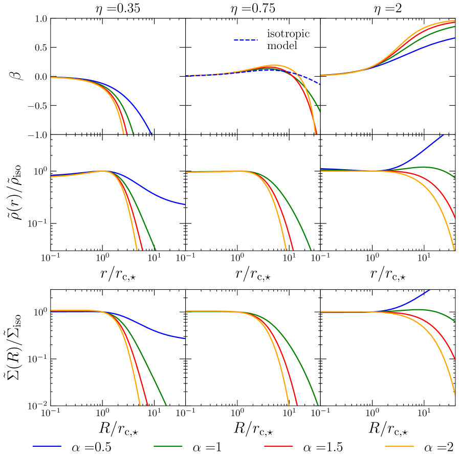
Fig.s 2 and 4 show how $\alpha$ and $\eta$ affect a model’s anisotropy and density profiles by comparing them with those of the reference isotropic model. The parameter $\eta$ mainly regulates the orbital anisotropy (Fig. 2 top row). Models are isotropic when $r\lesssim r_{\rm c,\star}$ because no model with a cored density distribution can be radially anisotropic inside the core (An & Evans 2006, Ciotti & Morganti 2010). In the outer regions, a model can be either tangentially or radially biased. Anisotropy is mildly enhanced by increasing $\alpha$: tangentially biased models become more tangential and radially biased models become more radial (Fig. 4 top row).

Let the normalized density profile be $\widetilde{\rho}\equiv\rho/\rho(r_{\rm c,\star})$ and the normalized surface density profile be $\widetilde{\Sigma}\equiv\Sigma/\Sigma(r_{\rm c,\star})$, and call these quantities for the isotropic model $\widetilde{\rho}_{\rm iso}$ and $\widetilde{\Sigma}_{\rm iso}$, respectively. Then the middle and bottom rows of Fig.s 2 and 4, show, respectively, the profiles of $\widetilde{\rho}/\widetilde{\rho}_{\rm iso}$ and $\widetilde{\Sigma}/\widetilde{\Sigma}_{\rm iso}$. We see that $\alpha$ and $\eta$ are degenerate in determining the density profile. Increasing $\alpha$ truncates the DF (4) more rapidly for large actions, while decreasing $\eta$ encourages orbits with high angular momentum. In either case, the outer density profile steepens. Increasing $\eta$ favours eccentric orbits and thus makes the density distribution slightly more cuspy (Fig. 2 middle row). Conversely, very tangentially biased models may present a density minimum at the centre (Fig. 4 middle left panel).

One could make $\eta$ a function of ${\bf J}$ to achieve greater flexibility in the anisotropy (see Williams & Evans 2015b), but the simple choice of constant $\eta$ provides significant flexibility (Fig.s 2 and 4), and avoids the introduction of new free parameters. We find empirically that models with $\eta>2$ or $\alpha>2$ have properties very similar to models with $\eta=2$ or $\alpha=2$, so we do not show them here.

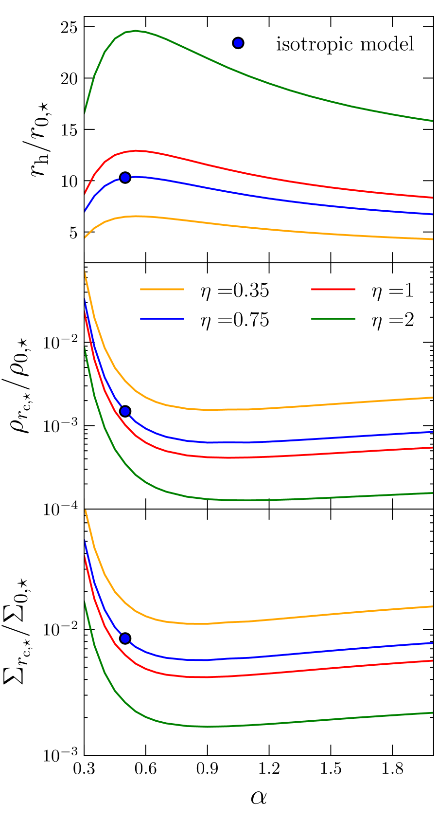
Fig. 4 shows how the physical scales $r_{\rm h}/r_{0,\star}$, $\rho_{r_{\rm c,\star}}/\rho_{0,\star}$ and $\Sigma_{r_{\rm c,\star}}/\Sigma_{0,\star}$ vary with ($\alpha,\eta$). Here $\rho_{r_{\rm c,\star}}\equiv\rho(r_{\rm c,\star})$, $\Sigma_{r_{\rm c,\star}}\equiv\Sigma(r_{\rm c,\star})$, $\rho_{0,\star}\equiv M_{\star}/r_{0,\star}^{3}$ and $\Sigma_{0,\star}\equiv M_{\star}/r_{0,\star}^{2}$. When $\eta$ is decreased at fixed $\alpha$, the model becomes more compact (middle row of Fig. 2), so $r_{\rm h}/r_{0,\star}$ decreases and $\rho/\rho_{0,\star}$ increases. While changing $\alpha$ at fixing $\eta$ affects the physical scaling only when $\alpha\lesssim 0.5$: in this regime, $r_{\rm h}/r_{0,\star}$ shortens (Fig. 4a) and models are slightly more cuspy, moving $\rho_{r_{\rm c,\star}}$ to higher values.

Figure 5: Kinematic observables in one-component models. Orange, red and blue curves are for models with to $\eta=0.35,0.75$ and $2$, respectively. Panels in the left column show line-of-sight velocity dispersions, normalized to $\sigma_{\rm los,R_{\rm e}}\equiv\sigma_{\rm los}(R_{\rm e})$, when $\alpha=0.5,1,2$. The other three panels show LOSVDs with the velocity scale normalized to $v_{c,R}$, the circular speed at the radius of observation $R$, which increases from left to right: $R=5\times 10^{-1}R_{\rm e}$, $R=R_{\rm e}$ and $R=3R_{\rm e}$. The value of $\alpha$ increases from top to bottom: $\alpha=0.5,1,2$.

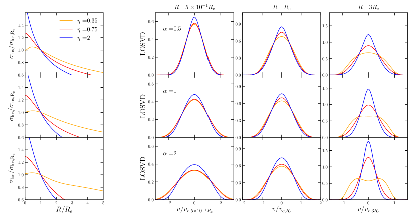
Fig. 5 plots the line-of-sight velocity dispersion profiles of models with different values of $\alpha$ and $\eta$, together with LOSVDs at three radii. The shape of a LOSVD encodes the velocity anisotropy: a flat-topped LOSVD indicates a tangentially biased system, while a radially biased system yields peaky LOSVDs. A wide LOSVD reflects highly populated nearly circular orbits: note how models with $\eta=0.35$ generate the widest LOSVDs. The model with $(\alpha,\eta)=(2,0.35)$ is an example of a model with extreme tangential anisotropy, in which the LOSVD is double-peaked around plus and minus the circular speed. This generates the flattest line-of-sight velocity dispersion profiles (Fig. 5, left column).

3.2 Spherical two-component models

We focus now on two-component spherical models, consisting of a stellar population with DF (4) and a dark halo with DF $f_{\rm dm}({\bf J})$. The adiabatic invariance of the actions makes them natural tools with which to analyse the addition of a stellar component to a dark halo. In the simplest scenario, gas falls into a dark halo over many dynamical times, so the dark halo contracts adiabatically. In this case the dark halo’s present configuration can be computed from its original DF $f({\bf J})$ without knowing how the rate of accretion of baryons varied over cosmic time. The dark halo is then predicted to have a very cuspy central structure, comprising particles with very small velocities. So, it would not be surprising if fluctuations in the gravitational potential generated by the baryons before most of them were driven out by supernovae had upscattered the least energetic dark-matter particles and thus erased the cusp (Navarro et al., 1996a; Governato et al., 2012; Nipoti & Binney, 2015; Read et al., 2019). For this reason we explore models with a dark-matter DF that, depending on the value of a parameter $J_{\rm c,dm}$, generates either a classical cuspy halo or a cored halo. This DF is (Cole & Binney, 2017; Pascale et al., 2018)

$$f_{\rm dm}({\bf J})=g_{\rm c}({\bf J})g_{\rm NFW}({\bf J})T({\bf J}),$$ (14)

where

$$g_{\rm c}({\bf J})=\biggl{[}\biggl{(}\frac{J_{\rm c,dm}}{h({\bf J})}\biggr{)}^{2}-\mu\frac{J_{\rm c,dm}}{h({\bf J})}+1\biggr{]}^{-5/6},$$ (15)

$$g_{\rm NFW}({\bf J})=\frac{g_{\rm dm}}{J_{0,\rm dm}^{3}}\frac{[1+J_{0,\rm dm}/h({\bf J})]^{5/3}}{[1+h({\bf J})/J_{0,\rm dm}]^{2.9}}$$ (16)

and

$$T({\bf J})=\exp{\biggl{[}-\biggl{(}\frac{h({\bf J})}{J_{\rm t,dm}}\biggr{)}^{2}\biggr{]}}.$$ (17)

Here $h({\bf J})$ is a homogeneous function of the actions of degree one

$$h({\bf J})=J_{r}+h_{\phi}|J_{\phi}|+h_{z}J_{z}.$$ (18)

The core action $J_{\rm c,dm}$ sets the spatial extent of the core in the density distribution, while $\mu$ is a dimensionless parameter used to make the dark-matter mass (14) independent of $J_{\rm c,dm}$ (Cole & Binney 2017). This convention is motivated by the idea that non-zero $J_{\rm c,dm}$ arises through dark-matter particles being upscattered but not ejected from the halo. $J_{\rm t,dm}$ is the truncation action, which serves to make normalization of the DF possible (equation 1).

We set the dimensionless parameters $h_{\phi}$ and $h_{z}$ to a common value $h$ so the DF (14) generates spherical models. In this case we cannot give an analytic expression for the constant $g_{\rm dm}$, which normalizes $f_{\rm dm}({\bf J})$ to unity. However, it can be readily computed following Appendix A of Pascale et al. (2018). The total dark matter mass $M_{\rm dm}$ together with the action scale $J_{0,\rm dm}$ define via equations (10) and (11) a scale radius $r_{0,\rm dm}$ and a scale velocity $v_{0,\rm dm}$.

Posti et al. (2015) showed that, in isolation, the DF (16) generates NFW-like models. The factor (15) was added by Cole & Binney (2017) to enable the DF to describe cored NFW models. The factor (17) was introduced by Pascale et al. (2018).

Table 1: Scale radii and corresponding circular speeds for one-component NFW haloes expressed in terms of the characteristic radius and velocity that follow from the halo’s DF (equations 10 and 11 with $\star$ replaced by dm). Equation (23) defines $r_{\rm s,dm}$.

$r_{\rm s,dm}/r_{0,\rm dm}$	$v_{c,\rm dm}(r_{\rm s,dm})/v_{0,\rm dm}$
0.67	0.40

As in Pascale et al. (2018), we define the dimensionless parameters

$$\widetilde{J}_{\rm c,dm}\equiv J_{\rm c,dm}/J_{0,\rm dm},$$ (19)

$$\widetilde{J}_{0,\rm dm}\equiv J_{0,\rm dm}/J_{0,\star}.$$ (20)

$$\widetilde{J}_{\rm t,dm}=J_{\rm t,dm}/J_{0,\rm dm},$$ (21)

and

$$\widetilde{M}_{\rm dm}\equiv M_{\rm dm}/M_{\star}.$$ (22)

Models sharing $\alpha$, $\eta$, $\widetilde{J}_{\rm c,dm}$, $\widetilde{J}_{0,\rm dm}$, $\widetilde{J}_{\rm t,dm}$, $\widetilde{M}_{\rm dm}$, $\mu$ and $h$ are homologous. The physical scales can be set a posteriori by choosing any pair among $M_{\rm dm},J_{0,\rm dm}$, $r_{0,\rm dm}$ and $v_{0,\rm dm}$. We introduce the logarithmic slope of the dark-matter density $\gamma_{\rm dm}\equiv\text{d}\ln\rho_{\rm dm}/\text{d}\ln r$, and define the halo scale radius $r_{\rm s,dm}$ from the relation

$$\gamma_{\rm dm}(r_{\rm s,dm})=-2,$$ (23)

as for the classical NFW model. The truncation and core radii are defined by

$$\gamma_{\rm dm}(r_{\rm t,dm})=-3,$$ (24)

and

$$\gamma_{\rm dm}(r_{\rm c,dm})=-{\textstyle\frac{1}{2}},$$ (25)

respectively.

3.2.1 Impact of stars on dark haloes

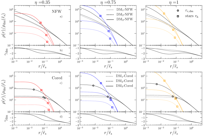
We consider representative stellar components with several orbital anisotropies, and examine the effects that cuspy or cored dark haloes and stars have on each other when they cohabit in the potential they jointly generate. we set $\alpha=0.5$ and select stellar DFs (4) that generate, in isolation, tangential, isotropic and radially biased models, by fixing $\eta=0.35,0.75$ and $1$, respectively (Section 3.1). For fixed $M_{\rm dm}$, we vary $M_{\star}$ to control the relative mass contribution $\widetilde{M}_{\rm dm}$. For both cuspy and cored haloes, and for each stellar anisotropy, we consider three groups of models, with $\widetilde{M}_{\rm dm}=10^{4},10^{3},10^{2}$. We refer to them as DM_i-NFW for the NFW haloes, and DM_i-Cored, for the cored haloes, with $i=1,2,3$, respectively. As $\widetilde{M}_{\rm dm}$ decreases, the stellar component becomes more massive. The chosen values of $\widetilde{M}_{\rm dm}$ generate models in which the dark halo strongly dominates over the stars in the central parts (DM₁, $\widetilde{M}_{\rm dm}(r_{\rm h})\gtrsim 20$), models in which stars and dark matter have similar density in the central parts (DM₂, $\widetilde{M}_{\rm dm}(r_{\rm h})\simeq 1$), and models in which the stars dominate in the central parts (DM₃, $\widetilde{M}_{\rm dm}(r_{\rm h})\lesssim 0.1$). In all groups the dark matter dominates far out. We do not explore different dark-halo anisotropies (for details, see Piffl et al. 2015) but set $h=1$, which makes the dark halo slightly radially biased. Also, $\widetilde{J}_{0,\rm dm}=3000$, which ensures $r_{\rm s,dm}/r_{\rm h}>1$ in all cases.

The exponential cut-off (17) introduces much freedom in setting $\widetilde{J}_{\rm t,dm}$, which, as long as it is large enough, does not affect the halo’s central properties. Thus, we standardize on $\widetilde{J}_{\rm t,dm}=20$, which truncates the halo density sufficiently far from the scale radius that it has no impact in the observationally accessible region ($r_{\rm t,dm}/r_{\rm s,dm}\gtrsim 30$). Once $\widetilde{J}_{\rm t,dm}$ and $h$ have been set for an NFW model, the DF’s physical scales follow unambiguously – Table 1 lists the values of $r_{\rm s,dm}/r_{0,\rm dm}$ and $v_{c,\rm dm}(r_{\rm s,dm})/v_{0,\rm dm}$ (i.e. the halo circular speed computed at $r_{\rm s,dm}$). The quantities $r_{\rm s,dm}$ and $v_{c,\rm dm}(r_{\rm s,dm})$ are available from cosmological simulations, and the pair ($r_{0,\rm dm}$, $v_{0,\rm dm}$) can be easily computed from Table 1 to scale any $f({\bf J})$ NFW-model onto the required scales. For the cored models we chose $\widetilde{J}_{\rm c,dm}=0.02$, which implies $\mu=0.2117$. The resulting core radius is $r_{\rm c,dm}\simeq 0.1r_{\rm s,dm}$. Table 2 summarizes the relevant parameters used to generate the presented models.

Fig. 6 plots, for our two-component models, the profiles of the dark matter (black curves) and stars (coloured curves), and also the dark-matter logarithmic density slopes $\gamma_{\rm dm}$ (long-thin bottom panels). Models with NFW haloes are plotted in the top row, while the bottom row shows models with cored haloes. The left column shows models with tangentially biased stellar components, while the rightmost column shows models in which the stellar component is radially biased. Dotted ($i=1$), dashed ($i=2$) and full ($i=3$) black lines show the dark haloes of models with increasingly massive stellar components. Whereas the dark haloes differ only modestly between $i=1$ and $i=2$, once the case $i=3,\widetilde{M}_{\rm dm}=10^{2}$ is reached, the stars’ gravity enhances the central density of the halo by a factor $\sim 10$ in the case of an NFW halo, and by a larger factor in the case of a cored halo. In all the $i=3$ models, the halo-steepness parameter hangs around $-2$ over a wide range of radii interior to $r_{\rm s,dm}$ with the consequence that the scale radius $r_{\rm s,dm}$ of these models is not uniquely defined. The steepening of $\gamma_{\rm dm}$ can reduce the core radii $r_{\rm c,dm}$ of cored models by a factor 10. The ratio $r_{\rm c,dm}/r_{\rm h}$ also reduces, by a factor $\sim 2$. This reduction diminishes the extent of the stellar system that is dominated by the halo’s core. Radially biased stellar components contract their dark haloes more strongly than tangential biased ones because radial bias increases the central star density (Fig.s 2, 4, and 4).

Figure 6: Density profiles of models with both stellar and dark-matter components with radii normalized to the scale radius $\widetilde{r}_{\rm s}$ of the corresponding one-component halo. Models shown in the upper row have NFW haloes, while models shown in the lower row have cored haloes. Table 2 lists the models’ parameters. The stellar mass fraction increases along the sequence dotted, dashed, full curves. DM profiles are plotted in black while stellar profiles are coloured. Squares indicate the half-mass radii of the stellar components, while in the lower row the black circles mark the DM core radii, defined by $\gamma_{\rm dm}(r_{\rm c,dm})=-1/2$.

3.2.2 Impact of dark haloes on stars

Table 2: Parameters used to generate the representative, two-component models: $h$, dimensionless parameter regulating the anisotropy of the dark halo; $\widetilde{J}_{0,\rm dm}$ and $\widetilde{J}_{\rm t,dm}$ as in equations (20) and (21); $\alpha$ and $\eta$, defined by the DF (4); $\widetilde{M}_{\rm dm}$ as in (22); $\widetilde{J}_{\rm c,dm}$, as in equation (19); $\mu$, dimensionless parameter used to make the normalization of the DF (14) independent of $J_{\rm c,dm}$.

$h$	$\widetilde{J}_{0,\rm dm}$	$\widetilde{J}_{\rm t,dm}$	$\alpha$	$\widetilde{M}_{\rm dm}$	$\eta$
1	3000	20	0.5	$10^{3}$-$10^{4}$-$10^{5}$	$0.35$-$0.75$-$1$
NFW models				Cored models
($\widetilde{J}_{\rm c,dm},\mu$)=(0,0)				($\widetilde{J}_{\rm c,dm},\mu$)=(0.02,0.2117)

Figure 7: Stellar kinematics in two-component models with NFW dark-matter haloes (equation 14). The stellar mass fraction increases along the sequence dotted, dashed, full curves. All models have $\alpha=0.5$ while $\eta$ increases from top to bottom ($\eta=0.35,0.75,1$) so the top and bottom models are tangentially and radially biased, respectively. The left column shows the anisotropy parameter, the centre column shows the LOSVD at $R=3R_{\rm e}$ normalized to the local velocity dispersion, and the right column shows $\sigma_{\rm los}$ normalized to its value at $R_{\rm e}$. In all models $\widetilde{J}_{0,\rm dm}=3000$, $\widetilde{J}_{\rm t,dm}=20$, $\widetilde{J}_{\rm c,dm}=0$, $\mu=0$, $h=1$, $\alpha=0.5$ (Table 2).

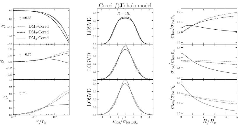
Fig.s 7 and 8 show, respectively, the impact NFW and cored haloes have on the kinematics of the stellar component. Again dotted, dashed and full curves relate to increasingly massive stellar components ($i=1,2,3$), and black, grey and light grey curves relate to tangentially biased, isotropic and radially biased stellar components. Addition of a dark halo changes the velocity anisotropy of the stellar component (left column) by decreasing the ratio $\Omega_{L}/\Omega_{r}$ at a given radius, and it is this ratio which sets the value of $\eta$ that corresponds to isotropy (equations 12 and 13). Since adding a halo diminishes the critical value of $\Omega_{L}/\Omega_{r}$, at fixed $\eta$ it increases radial bias (broken curves above full curves in left columns of Fig.s 7 and 8). This effect is most pronounced at $r\gg r_{\rm h}$, where the potential of a one-component model is almost Keplerian.

These changes in $\beta$ make the LOSVD at $R=3R_{\rm e}$, shown in the central columns, more peaky, but the effect is quite weak and would be very hard to detect observationally. The right columns plot $\sigma_{\rm los}(R)$, which is significantly flattened by the addition of a massive dark halo, a consequence of adiabatic compression of the envelope of the stellar system by the very extended dark-matter distribution.

Figure 8: As Fig. 7 except for models with cored haloes (see Table 2).

3.3 Effects of a central massive black hole

Here we explore how stellar components with the DF (4) are modified by a central massive black hole (hereafter BH). We present models with and without a dominating dark halo. The potential of the BH is taken to be that of a Plummer model

$$\Phi_{\rm BH}=-\frac{GM_{\rm BH}}{\sqrt{r^{2}+a^{2}}},$$ (26)

with $a$ too small to impact any observable.

We choose two representative stellar components with $\alpha=0.5$ that, in isolation, are quasi-isotropic ($\eta=0.75$) and radially biased ($\eta=1$). When a dark halo is included, its parameters are those of the DM₂-NFW model (Section 3.2.1, Table 2). We consider BH masses of $\mu_{\rm BH}\equiv M_{\rm BH}/M_{\star}\equiv 0.001,0.0017,0.005$ (Magorrian et al. 1998). The BH’s radius of influence $R_{\rm infl}$ is the projected distance on the plane of the sky within which the BH’s gravity cannot be neglected. We define it such that (Binney & Tremaine 2008)

$$\sigma_{\rm los,\star}(R_{\rm infl})=\sqrt{\frac{GM_{\rm BH}}{R_{\rm infl}}},$$ (27)

where $\sigma_{\rm los,\star}$ is the stars line-of-sight velocity dispersion. Table 3 lists the parameters of our models, including $R_{\rm infl}$.

Table 3: Main parameters of models with BHs. The stellar DF has the form (4) and the BH’s potential is given by (26). If the model has dark halo, its (NFW) DF is given by (14). All models have $\alpha=0.5$ and $\eta$ controls the stellar anisotropy. The BH-to-stellar mass fraction is $\mu_{\rm BH}=M_{\rm BH}/M_{\star}$. Equation (27) defines the radius of influence $R_{\rm infl}$, which is given as a fraction of the stellar effective radius. For models with dark matter, the quantities defined by equations (21), (22) and (20) are $\widetilde{J}_{\rm t,dm}=20$, $\widetilde{M}_{\rm dm}=1000$, $\widetilde{J}_{0,\rm dm}=3000$. $M_{\star}$ and $J_{0,\star}$ can be scaled to any values of interest.

		no DM	with DM
$\eta$	$\mu_{\rm BH}$	$R_{\rm infl}/R_{\rm e}$	$R_{\rm infl}/R_{\rm e}$
	0.005	$2.81\times 10^{-2}$	$9.67\times 10^{-3}$
0.75	0.0017	$9.87\times 10^{-3}$	$3.31\times 10^{-3}$
	0.001	$6.02\times 10^{-3}$	$2.00\times 10^{-3}$
	0.005	$2.43\times 10^{-2}$	$9.94\times 10^{-3}$
1	0.0017	$8.60\times 10^{-3}$	$3.40\times 10^{-3}$
	0.001	$5.24\times 10^{-3}$	$2.05\times 10^{-3}$

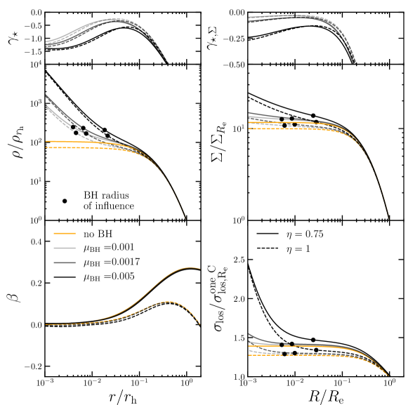
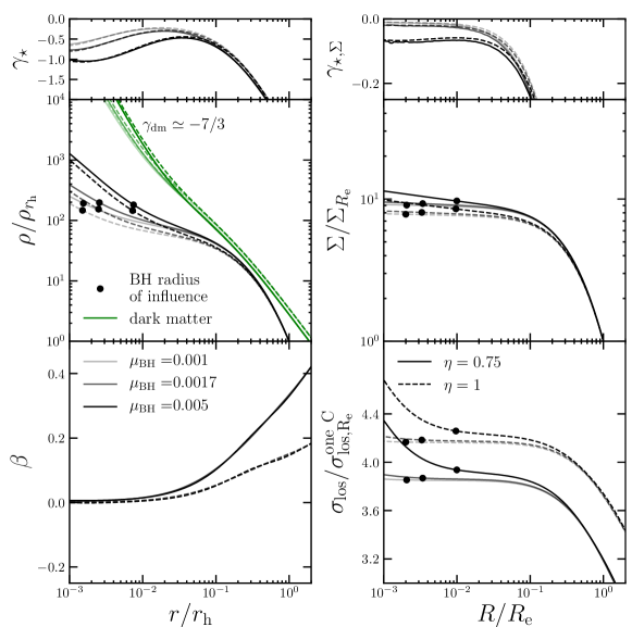
Fig. 9 plots stellar properties of the models without dark haloes. The left column plots three three-dimensional diagnostics: from top to bottom logarithmic slope $\gamma_{\star}$, density $\rho$ and anisotropy $\beta$. The right column plots projected quantities: from top to bottom logarithmic slope $\gamma_{\star,\Sigma}\equiv\text{d}\ln\Sigma/\text{d}\ln R$, surface density $\Sigma$ and velocity dispersion $\sigma_{\rm los}$ in units of the line-of-sight velocity dispersion at $R_{\rm e}$ in the corresponding one-component model. Solid and dashed lines relate to models with $\eta=0.75$ ($\sim$isotropic) and 1 (radially biased), respectively. Values of $\mu_{\rm BH}$ increase from bottom to top, with orange curves showing models without BHs. Black points mark values of $R_{\rm infl}$.

It is evident that $R_{\rm infl}$ is essentially proportional to $\mu_{\rm BH}$ and insensitive to $\eta$ (Table 3). It is also evident that on the sky the region that is significantly affected by the BH is much smaller than the corresponding three-dimensional region. In the latter, the stellar density becomes very cuspy, with $\gamma_{\star}$ approaching $-1.5$ as predicted by previous works (Quinlan et al., 1995; Binney & Tremaine, 2008). At $R_{\rm infl}$ the logarithmic slope of the projected density profile $\gamma_{\star,\Sigma}(R_{\rm infl})\simeq-0.13$ in the model with the highest $\mu_{\rm BH}$. The central divergence of the line-of-sight velocity dispersion is $\sigma_{\rm los}\simeq r^{-1/2}$, as expected, but sets in only well inside $R_{\rm infl}$. The bottom left panel of Fig. 9 shows that the models remain isotropic at their centres (Goodman & Binney, 1984).

Fig. 10 plots the same quantities as Fig. 9 but for the models with a dominant dark halo. In a model with both stars and a dark halo, the slopes of the cusps that the BH creates in each component are the same ($\rho_{\star}\sim r^{-3/2}$, $\rho_{\rm dm}\sim r^{-7/3}$, Quinlan et al. 1995) as those created by BHs in single-component models. The main effect of adding a dark halo is to increase the stellar velocity dispersion before addition of a BH, with the consequence that the dynamical impact of the BH is confined to smaller radii than in a model without a dark halo; $R_{\rm infl}$ shrinks by a factor 2–3 (Table 3). The change in the outer stellar velocity distributions (Fig. 10, bottom panel, left column) is only due to different $\Omega_{L}/\Omega_{r}$ set by the dark halo (see Section 3.2.2).

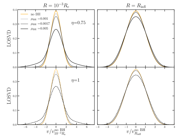
Fig. 11 shows stellar LOSVDs for models without dark matter, computed at both $R=R_{\rm infl}$ (left column) and $R\simeq 10^{-3}R_{\rm e}$. There are substantial differences between the LOSVDs with different $\mu_{\rm BH}$ only at the smaller radius.

These models underline the need for exquisitely accurate surface brightness profiles and velocity measurements to well inside $R_{\rm infl}$ if intermediate massive BHs (IMBHs) are to be detected in GCs and dSphs. In GCs, $R_{\rm infl}$ is often already close to the smallest currently resolvable spatial scale. For instance: if $\omega$ Centauri, one of the largest GCs with $r_{\rm h}\simeq 5\,$arcmin (Harris 1996) and a good candidate to host an IMBH (van der Marel & Anderson, 2010), contained a BH with $\mu_{\rm BH}=0.005$, $R_{\rm infl}$ would be of the order of 10 arcsec (assuming $r_{\rm h}\simeq R_{\rm e}$, Table 3). Moreover, extreme crowding, the problem of locating the centre of a system, and the possibility that any inward increase in the velocity dispersion is driven by mass segregation rather than a BH, all make it hard to build a convincing case for an IMBH in a GC (Zocchi et al., 2019). We have shown that the dark haloes of dSphs make the problem harder in dSphs by driving $R_{\rm infl}$ inwards.

Figure 9: Impact of a central black hole of mass $\mu_{\rm BH}\equiv M_{\rm BH}/M_{\star}$ on two one-component models. A model with $\eta=0.75$ is shown by full curves while dashed curves show the radially biased model with $\eta=1$. Both models have $\alpha=0.5$. Colours indicate BH mass fraction: orange for no black hole, greys for $\mu_{\rm BH}=0.001,0.0017,0.005$, respectively. Panels in the left column show from top to bottom: logarithmic slope of the stellar density profile $\gamma_{\star}$; stellar density; anisotropy parameter. Panels in the right column show: logarithmic slope of the projected density slope profile $\gamma_{\star,\Sigma}$; projected density; line-of-sight velocity dispersion. Black points mark values of $R_{\rm infl}$. Densities are normalized to $\rho_{r_{\rm h}}\equiv\rho(r_{\rm h})$, surface densities to $\Sigma_{R_{\rm e}}\equiv\Sigma(R_{\rm e})$ and line-of-sight velocity dispersions to $\sigma^{\rm one\ C}_{\rm los,R_{\rm e}}$, the line-of-sight dispersion of the one component model, computed at $R=R_{\rm e}.$

Figure 10: Same as Fig. 9 except for models with an NFW dark halo. The green curves in the centre left panel show the density of DM. All grey and black curves refer to the stars.

Figure 11: The impact of a BH on LOSVDs in one-component models: upper row an isotropic model ($\eta=0.75$); lower row a radially biased model ($\eta=1$); left column LOSVD at $R=10^{-3}R_{\rm e}$; right column LOSVD at $R=R_{\rm infl}$. Black hole mass fractions from zero to $0.005$ are indicated by line type. Velocities are normalized to the line-of-sight velocity dispersion at the relevant radius, $v_{R}^{\rm no\,BH}$, with $R=10^{-3}R_{\rm e},R_{\rm infl}$, respectively in the left and right columns. The orange curves show the LOSVD of the corresponding model with no BH. In this case $R_{\rm infl}$ is not defined so we plot the LOSVD at $10^{-2}R_{\rm e}$.

4 Application to data

We have indicated that the DF (4) has all the required features to model the typically observed properties of dSphs and GCs. In this Section we justify this statement.

Fitting models to data for a specific object involves careful consideration of issues with the data such as degradation by seeing, foreground contamination, selection effects associated with crowding or field-of-view limitations and selection of bright stars for spectroscopy. Consequently, presentation of a thorough fitting exercise of a single system would shift the focus from the DF (4) to the fitted system. Presentation of the same exercise for several diverse systems is not feasible in a single paper. Hence we do not attempt detailed fits. Instead, we plot alongside data the predictions of a variety of models in the hope of convincing readers that there are models within the set explored that would provide acceptable fits to the data after correction of all relevant observational biases.

4.1 Globular Clusters

Figure 12: One-component models of globular clusters. From left to right: $\omega$ Centauri, NGC 5904, NGC 5024, NGC 7089. The upper panels show data and model predictions for surface brightness. Curves show the models that fit the data best for pre-determined anisotropy: $\eta$= 0.5 (green), 0.75 (grey), 1 (blue), 1.5 (red). The models’ line-of-sight velocity dispersion profiles, scaled to match the observed line-of-sight velocity dispersion profiles (Baumgardt et al. 2019), are shown in the bottom panels. For each model we report the value of the reduced chi squared $\tilde{\chi^{2}}$.

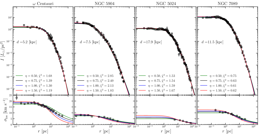
We chose four representative GCs: $\omega$ Centauri, NGC 5904, NGC 5024 and NGC 7089. To demonstrate the flexibility of the DF (4), we fit the surface brightness profiles of each GC with four one-component models, each with a different velocity anisotropy.

Cluster distances are taken from the Harris (1996) catalogue, the surface brightness profiles from the catalogue of Trager et al. (1995), while the line-of-sight velocity dispersion profiles from Baumgardt et al. (2019). The surface brightness data sets consist of triplets of $\{R_{i},I^{\rm obs}_{i},\delta I_{i}\}$, with $i=1,...,N$, where $R_{i}$ is the $i$-th bin’s average radius and $I_{i}$ and $\delta I_{i}$ are its surface brightness and error. The errors are computed following Section 2.2 of McLaughlin & van der Marel (2005). The line-of-sight velocity dispersion profiles consist of triplets $\{R_{k},\sigma_{\rm los,k},\delta\sigma_{\rm los,k}\}$, with $k=1,...,M$, where $R_{k}$ is the bin’s avarage radius, while $\sigma_{\rm los,k}$ and $\delta\sigma_{\rm los,k}$ are its line-of-sight velocity dispersion and error, respectively.

We present models with $\eta$ = 0.5, 0.75, 1, 1.5, to cover a wide range of anisotropies (see Section 3.1). To determine the best fitting model, we minimize the chi squared

$$\chi^{2}\equiv\sum_{n=1}^{N}\biggl{(}\frac{I^{\rm mod}_{i}(R_{i})-I^{\rm obs}_{i}}{\delta I_{i}}\biggr{)}^{2}.$$ (28)

Since equation (28) does not include the fit to the kinematics, the only free parameters to be constrained by data are $\alpha$, $r_{0,\star}$ and a normalization parameter $Q\equiv M_{\star}/\varUpsilon_{\star}$, where $\varUpsilon_{\star}$ is the mass-to-light ratio. The mass scale $M_{\star}$ of each model is then determined by fitting the observed GC velocity dispersion profile only.

Given the few free parameters, we adopt a uniform grid search method to find the minimum of (28). The model surface brightness $I_{i}^{\rm mod}(R_{i})$ is computed assuming a constant mass-to-light ratio $\varUpsilon_{\star}$. The value of $\varUpsilon_{\star}$ is unambiguously determined by the requirement that the model provides the total luminosity..

The upper panels of Fig. 12 show that for all four values of $\eta$ one can fit the very precise photometric data almost perfectly, even though the data extend over nearly five orders of magnitude in surface brightness. As measure of the goodness of the fits, Fig. 12 lists the values of the reduced chi square, $\tilde{\chi}^{2}\equiv-\chi^{2}/$d.o.f., where d.o.f. = $N$ - 2. The only slight misfit is at the centre of NGC 5904, where a mild cusp in the data cannot be reproduced by the DF (4). The lower panels of Fig. 12 show the line-of-sight velocity dispersion profiles of the models scaled to match the observed profiles. The shape of the line-of-sight velocity dispersion profiles of each GC is well reproduced by at least one model. The parameters of these models are listed in Table 4.

While we have demonstrated that the application of the DF (4) to GCs is promising, our one-component models can only be regarded as starting points for a much more sophisticated modelling effort. All GCs have experienced significant mass segregation. Consequently, stars of different masses and evolutionary stage will be distributed differently in action space. In particular, more massive stars will be more tightly clustered towards the origin of action space than less massive stars. Black holes and neutron stars, will be most tightly clustered around the origin, followed by horizontal-branch stars, followed by turnoff stars. Low-mass main-sequence stars will extend furthest from the origin of action space. Each stellar type should have its own DF $f({\bf J})$ and be an independent component of a composite model (Gieles & Zocchi, 2015; Zocchi et al., 2016). The observables such as surface brightness and line-of-sight velocity dispersion would be predicted by weighting these components according to their luminosity. Many GCs show significant signs of rotation (Bianchini et al. 2018), and to reproduce this aspect of the observations we would need to include in the DF a component odd in $J_{\phi}$ (Binney 2014, see also Jeffreson et al. 2017 who used a different family of action-based DFs to reproduce flattened, rotating and almost isotropic GCs).

Table 4: Parameters of the models fitted to GC data. $\eta$ and $\alpha$ are dimensionless parameters in the DF (4). $J_{0,\star}$ is the action scale, while $M_{\star}$ is the total mass. $M_{\star}/L_{\rm V}$ is the mass-to-light ratio, with $L_{\rm V}$ the total luminosity in the V band, taken from Harris (1996). $\chi^{2}$ of the best-fitting model is defined by equation (28). $N$ is number of bins in the observed surface brightness profile.

$\omega$ Centauri ($N$=51)
$\eta$	$\alpha$	$J_{0,\star}$ [kpc km s-1]	$M_{\star}$ [$10^{5}M_{\odot}$]	$M_{\star}/L_{\rm V}$	$\chi^{2}$
0.5	$0.931$	2.15	34.8	3.20	84.51
0.75	$0.954$	2.87	31.7	2.91	68.22
1	$1.02$	3.78	29.2	2.69	63.88
1.5	$1.26$	6.59	26.3	2.42	58.40
NGC 5904 ($N$=78)
$\eta$	$\alpha$	$J_{0,\star}$ [kpc km s-1]	$M_{\star}$ [$10^{5}M_{\odot}$]	$M_{\star}/L_{\rm V}$	$\chi^{2}$
0.5	0.503	$6.70\times 10^{-2}$	3.06	1.07	216.92
0.75	0.522	$1.08\times 10^{-1}$	2.98	1.04	182.09
1	0.543	$1.55\times 10^{-1}$	2.88	1.00	161.60
1.5	0.605	$3.15\times 10^{-1}$	2.72	0.95	139.98
NGC 5024 ($N$=111)
$\eta$	$\alpha$	$J_{0,\star}$ [kpc km s-1]	$M_{\star}$ [$10^{5}M_{\odot}$]	$M_{\star}/L_{\rm V}$	$\chi^{2}$
0.5	0.464	$1.25\times 10^{-1}$	2.54	0.98	166.82
0.75	0.480	$2.18\times 10^{-1}$	2.94	1.13	168.15
1	0.502	$3.60\times 10^{-1}$	3.30	1.27	172.87
1.5	0.556	$8.50\times 10^{-1}$	3.96	1.52	181.53
NGC 7089 ($N$=82)
$\eta$	$\alpha$	$J_{0,\star}$ [kpc km s-1]	$M_{\star}$ [$10^{5}M_{\odot}$]	$M_{\star}/L_{\rm V}$	$\chi^{2}$
0.5	0.500	$2.29\times 10^{-1}$	7.83	2.24	60.34
0.75	0.517	$3.62\times 10^{-1}$	7.85	2.24	50.45
1	0.540	$5.55\times 10^{-1}$	7.90	2.26	48.77
1.5	0.600	1.14	7.84	2.24	49.58

4.2 Dwarf spheroidal galaxies

Pascale et al. (2018) demonstrated that the DF (4) yields very accurate models of the Fornax dSph. Here we model five further dSphs: Carina, Leo I, Sculptor, Sextans and Ursa Minor, with the aim to prove that the use of the DF (4) can be extended to the whole population of classical dSphs. We present spherical, anisotropic models, with separate DFs for the stellar and the halo components, which just fit the dSph number density profiles, given a certain orbital anisotropy. For Sculptor we present three-component models, which have distinct DFs for the red and blue horizontal branch stars and the dark matter halo.

The projected number density profiles of the Carina, Leo I, Sextans and Ursa Minor dSphs have been taken from Irwin & Hatzidimitriou (1995), while their line-of-sight velocity dispersion profiles are from Walker et al. (2007). The projected number density and line-of-sight velocity dispersion profiles of the distinct populations of Sculptor are from Battaglia et al. (2008). We adopt distances from Mateo (1998).

4.2.1 Carina, Leo I, Sextans and Ursa Minor

Our analysis proceeds essentially as described in Section 4.1. The photometric contribution is now computed from triplets $\{R_{i},n_{\star,i}^{\rm obs},\delta n_{\star,i}^{\rm obs}\}$, where $n_{\star,i}^{\rm obs}$ and $\delta n_{\star,i}^{\rm obs}$ are a number density and its error. The predicted number density, $n_{\star}^{\rm mod}$, is computed from the surface density of mass assuming a constant mass per detected star, $\overline{m}$. The kinematics is computed from triplets $\{R_{k},\sigma_{{\rm los},k},\delta\sigma_{{\rm los},k}\}$. The stellar component of each dSph is represented by DF (4), with fixed stellar masses $M_{\star}$ (see Table 5). The dark matter halos are described by the cuspy DF (14, $\widetilde{J}_{\rm c,dm}=0$). For each dSph with stellar mass $M_{\star}$, according to estimetes of the low mass end of the stellar-to-halo mass relation (Read et al., 2017), and to the halo-mass concentration ralation (Muñoz-Cuartas et al., 2011), we fix the dark matter mass enclosed within the halo scale radius $M_{\rm dm}(<r_{\rm s,dm})$, and the halo scale radius $r_{\rm s,dm}$, to values predicted by cosmology. The prescribed values of $M_{\rm dm}(<r_{\rm s,dm})$ and $r_{\rm s,dm}$ are obtained by varying iteratively $M_{\rm dm}$ and $J_{0,\rm dm}$ (the final values of these parameters are given in Table 5).

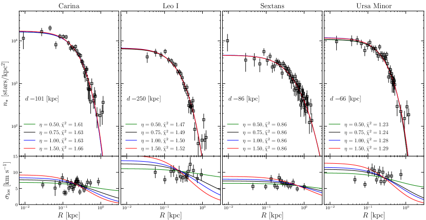
The upper panels of Fig. 13 show that for all four values of $\eta$ the best DF provides an excellent fit to the observed number density profiles of the four galaxies. The lower panels shows the observed velocity dispersion profiles of the galaxies alongside the predictions for each value of $\eta$.

Table 5 gives the values of the parameters and of $\chi^{2}$ for the best-fitting models of Carina, Leo I, Sextans and Ursa Minor. It also gives the parameters and $\chi^{2}$ for the best-fitting Sérsic (1968) profile

$$n_{S}(R)=n_{0}\exp\biggl{[}-\biggl{(}\frac{R}{R_{S}}\biggr{)}^{1/m}\biggr{]}.$$ (30)

Every DF yields a comparable or lower $\chi^{2}$ than does the Sérsic profile. This is remarkable in as much as (i) fits of both the DF and the Sérsic profile require searches over just two parameters in addition to a basic scaling parameter, yet (ii) the DF defines a complete, dynamically consistent six-dimensional model whereas the Sérsic profile provides nothing beyond the radial run of density. Consequently, it can be argued that a dSph is more effectively described by the parameters of its best-fitting $f({\bf J})$ than by the parameters of the best-fitting Sérsic profile.

Figure 13: Models of dSphs with a stellar comonent and a dark matter halo. Columns from the left to right: Carina, Leo I, Sextans, Ursa Minor. Upper panels show projected number densities together with fits by four models with pre-determined stellar velocity anisotropy: $\eta$= 0.5 (green), 0.75 (grey), 1 (blue), 1.5 (red). The parameters of the models are reported in Table 5. Lower panels show observed line-of-sight velocity dispersions and the models’ predictions. For each model we report the value of the reduced chi squared.

4.2.2 Sculptor

Figure 14: Three-component models of the Sculptor dSph (two stellar components and a dark matter halo). The velocity anisotropy of the stellar components is slightly radially biased ($\eta=0.75$) in the left column and radially biased ($\eta=1$) in the right column. Red and blue curves in the upper panels show model fits to the observed surface densities of RHB and BHB, respectively. The lower panels show the predicted line-of-sight velocity dispersion profiles of each component alongside the observed profiles.

dSphs usually exhibit complex star formation and chemical enrichment histories. These galaxies seem to experience bursts of star formation, and the stars formed in each burst are distributed differently in action space. Since all populations move in a common potential, observations that are able to distinguish between the populations have the potential to constrain the system’s gravitational field more strongly than is possible in a system with only a single population (Walker & Peñarrubia, 2011; Agnello & Evans, 2012; Amorisco et al., 2013).

We model two populations in the Sculptor dSph, with each population described by the DF (4), and with a separate component describing a dark matter halo DF (14). The two populations are the stars on the blue (red) horizontal branch BHB (RHB), which are less (more) metal rich and more (less) extended spatially.

We will refer to all the parameters belonging to the BHB (RHB) populations, as $\ast^{\rm BHB}$ ($\ast^{\rm RHB}$) where $\ast$ = $\alpha$, $\eta$, $M_{\star}$, $J_{0,\star}$. For simplicity in each model $\eta$ is the same for both populations and the total stellar mass $M_{\star}^{\rm BHB}+M_{\star}^{\rm RHB}$ is fixed. We consider two representative cases, $\eta=0.75$ (slightly radially biased) and $\eta=1$ (radially biased). We assume a cored dark matter halo described by DF (14; $\widetilde{J}_{\rm c,dm}=0.02$). As for the other dSphs, we fix the enclosed mass $M_{\rm dm}(<r_{\rm s,dm})$ and the scale radius $r_{\rm s,dm}$ to cosmologically motivated values.

Then the model’s free parameters are

$$\boldsymbol{\xi}=\biggl{(}\alpha^{i},J_{0,\star}^{i},\frac{M_{\star}^{\rm BHB}}{M_{\star}^{\rm BHB}+M_{\star}^{\rm RGB}},J_{0,\rm dm},M_{\rm dm}\biggr{)},\quad(i=\hbox{RHB, BHB}).$$ (31)

We minimize the figure of merit

$$\chi^{2}_{\rm tot}=\chi^{2}_{\rm RHB}+\chi^{2}_{\rm BHB},$$ (32)

where $\chi^{2}$ for each population is defined by equation (28).

In view of the higher dimensionality of this problem, we explored the parameter space using a stochastic search method based on a Markov-Chain Monte Carlo (MCMC) algorithm, with a Metropolis-Hastings (Metropolis et al. 1953, Hastings 1970) sampler, to sample from the posterior distribution. We used uninformative, flat priors on the free parameters (31).

In the upper panels of Fig. 14 squares and circles mark the number densities of BHB and RHB stars, respectively. The predictions for these populations of the best-fitting models are shown by blue and red curves, respectively. The left panel shows the fit provided by the mildly radially biased model, and the right panel shows the fit provided by the radially biased model. It is clear that both three-component models provide excellent fits to the data, and that also the models predictions on the line-of-sight velocity dispersion profiles provide an excellent description of the data. Table 6 gives the models’ parameters.

These simple test cases prove that the extension of the DF (4) to the whole system of classical dSphs is possible and promising, whether the galaxy is represented as a single stellar population or in more sophisticated model that reflects the chemodynamic history of the system.

Table 5: Parameters of two-component models fitted to dwarf spheroidal galaxies.$\eta$ and $\alpha$ are dimensionless parameters in the DF (4). $J_{0,\star}$ is the action scale while $M_{\star}$ is the dSph total mass: ¹ Ural et al. (2015), ² Weisz et al. (2014), ³ Karlsson et al. (2012). $M_{\rm dm}$ and $J_{0,\rm dm}$ are the halo total mass and action scale equation (14). The dark halo DF is cuspy, with $\widetilde{J}_{\rm c,dm}=0$. The figure of merit $\chi^{2}$ of the best-fitting model is defined by equation (28). $N$ is number of bins in the observed star-count profile. $n_{0}$, $m$ and $R_{S}$ are the normalization, Sérsic index and scale radius, respectively, of the best-fitting Sérsic profile (equation 30).

Carina ($N$=36)
$f({\bf J})$ model						Sérsic Fit
$\eta$	$\alpha$	$J_{0,\star}$ [kpc $\,{\rm km\,s}^{-1}$]	$M_{\star}$ [10${}^{6}\,M_{\odot}$]	$M_{\rm dm}$ [10${}^{8}\,M_{\odot}$]	$J_{0,\rm dm}$ [kpc $\,{\rm km\,s}^{-1}$]	$\chi^{2}$	$n_{0}$ $[n_{\star}$ kpc${}^{-2}]$	$m$	$R_{s}$ [kpc]	$\chi^{2}$
0.5	0.946	0.677	0.481	8.69	44.58	56.42	14.17	0.813	0.215	57.42
0.75	1.10	1.21				56.88
1	1.33	1.96				57.11
1.5	1.81	3.48				57.90
Leo I ($N$=31)
$\eta$	$\alpha$	$J_{0,\star}$ [kpc $\,{\rm km\,s}^{-1}$]	$M_{\star}$ [10${}^{6}\,M_{\odot}$]	$M_{\rm dm}$ [10${}^{9}\,M_{\odot}$]	$J_{0,\rm dm}$ [kpc $\,{\rm km\,s}^{-1}$]	$\chi^{2}$	$n_{0}$ $[n_{\star}$ kpc${}^{-2}]$	$m$	$R_{s}$ [kpc]	$\chi^{2}$
0.5	0.714	0.513	5.52	6.57	174.3	44.03	38.03	0.876	0.182	44.80
0.75	0.860	1.18				44.63
1	0.933	1.74				44.87
1.5	1.34	4.20				45.52
Sextans ($N$=56)
$\eta$	$\alpha$	$J_{0,\star}$ [kpc $\,{\rm km\,s}^{-1}$]	$M_{\star}$ [10${}^{6}\,M_{\odot}$]	$M_{\rm dm}$ [10${}^{8}\,M_{\odot}$]	$J_{0,\rm dm}$ [kpc $\,{\rm km\,s}^{-1}$]	$\chi^{2}$	$n_{0}$ $[n_{\star}$ kpc${}^{-2}]$	$m$	$R_{s}$ [kpc]	$\chi^{2}$
0.5	0.594	0.420	0.53	7.94	47.0	47.31	3.33	1.13	0.339	48.54
0.75	0.656	0.828				47.39
1	0.724	1.41				47.40
1.5	0.902	3.33				47.33
Ursa Minor ($N$=37)
$\eta$	$\alpha$	$J_{0,\star}$ [kpc $\,{\rm km\,s}^{-1}$]	$M_{\star}$ [10${}^{6}\,M_{\odot}$]	$M_{\rm dm}$ [10${}^{9}\,M_{\odot}$]	$J_{0,\rm dm}$ [kpc $\,{\rm km\,s}^{-1}$]	$\chi^{2}$	$n_{0}$ $[n_{\star}$ kpc${}^{-2}]$	$m$	$R_{s}$ [kpc]	$\chi^{2}$
0.5	1.17	1.54	0.292	1.316	50.7	44.43	3.62	0.665	0.278	42.743
0.75	1.39	2.61				44.82
1	1.32	2.94				46.00
1.5	2.20	6.03				46.42

Table 6: Parameters of DFs fitted to three components the Sculptor dwarf spheroidal galaxy. $\eta^{\rm pop}$ and $\alpha^{\rm pop}$ are dimensionless parameters in the DF (4). $J_{0,\star}^{\rm pop}$ is the scale action defined by the DF. $M_{\star}^{\rm pop}$ the component’s mass. $J_{0,\rm dm}$ and $M_{\rm dm}$ are the halo action scale and total mass (equation 14). The dark halo DF (14) is cored, with $\widetilde{J}_{\rm c,dm}=0.02$. The figure of merit $\chi^{2}$ of the best-fitting model is defined by equation (28). The BHB and RHB star-count profiles have a number of bin $N^{\rm BHB}=23$ and $N^{\rm RHB}=11$, respectively. The total stellar mass $M_{\star}^{\rm BHB}+M_{\star}^{\rm RHB}=2.3\times 10^{6}\,M_{\odot}$ Weisz et al. 2014.

Sculptor
$\eta^{\rm BHB}=\eta^{\rm RHB}$	$\alpha^{\rm BHB}$	$J_{\star,0}^{\rm BHB}$ [kpc $\,{\rm km\,s}^{-1}$]	$\alpha^{\rm RHB}$	$J_{\star,0}^{\rm RHB}$ [kpc $\,{\rm km\,s}^{-1}$]	$\frac{M_{\star}^{\rm BHB}}{M_{\star}^{\rm BHB}+M_{\star}^{\rm RHB}}$	$J_{0,\rm dm}$ [kpc $\,{\rm km\,s}^{-1}$]	$M_{\rm dm}$ [$10^{9}\,M_{\odot}$]	$\chi^{2}$
0.75	0.591	0.389	1.83	1.86	0.892	148.2	5.87	49.50
1	0.554	0.359	2.41	2.79	0.736	167.8	7.36	46.09

5 Conclusions

As we acquire more complete data for galaxies and star clusters, more sophisticated models are required to fit the data well and to provide predictions for further observations that can be tested by extending the available data. Full exploitation of the best current data requires models that (i) include several components and (ii) predict not just velocity moments but full LOSVDs. Models that meet these criteria are readily constructed if we use action integrals as the arguments of the DF. A self-consistent model that provides a good fit to a given system can be quickly constructed by allocating each component, disc, stellar halo, dark halo, etc., a DF with an appropriate functional form. In this paper we have explored the scope of the DF (4) that was introduced by Pascale et al. (2018) to model the Fornax dSph. This DF complements DFs previously introduced by Binney (2010) and Posti et al. (2015) in yielding spheroidal systems with exponential density profiles.

The DF has two key parameters, $\eta$ and $\alpha$, which principally control velocity anisotropy and the radial density profile, respectively. We have explored models that contain only stars and models that also have a dark halo. We have investigated the impact that the dark halo has on stellar observables both when the halo has been adiabatically distorted by the stars from the classic NFW form, and when dark-matter particles have been scattered out of low-action orbits to form a dark core. We have also explored models in which a massive BH sits at the centre of the galaxy.

We have shown that models generated by the Pascale et al. (2018) DF provide excellent fits to both globular clusters and to four dSph galaxies. The surface-brightness profiles can be fitted equally well with models that have a wide range of velocity anisotropies, from radially to tangentially biased. These models provide an extremely convenient platform from which to explore that potential of observations to detect dark matter and IMBHs in globular clusters or dSphs. We have also presented a three-component model of the Sculptor dSph that describes perfectly the different spatial extents of the stars on the blue and red horizontal branches, again for a wide range of assumed velocity anisotropies.

The models presented are all been non-rotating and spherical. One of the strengths of the $f({\bf J})$ modelling technique is the ease with which a spherical model can be flattened and set rotating (Binney, 2014), and a forthcoming paper will explore rotating and flattened models systematically

References

- Agnello & Evans (2012) Agnello A., Evans N. W., 2012, ApJ, 754, L39
- Amorisco et al. (2013) Amorisco N. C., Agnello A., Evans N. W., 2013, MNRAS, 429, L89
- An & Evans (2006) An J. H., Evans N. W., 2006, ApJ, 642, 752
- Arnold (1978) Arnold V. I., 1978, Mathematical methods of classical mechanics. Springer, New York
- Battaglia et al. (2008) Battaglia G., Helmi A., Tolstoy E., Irwin M., Hill V., Jablonka P., 2008, ApJ, 681, L13
- Baumgardt et al. (2019) Baumgardt H., Hilker M., Sollima A., Bellini A., 2019, MNRAS, 482, 5138
- Bianchini et al. (2018) Bianchini P., van der Marel R. P., del Pino A., Watkins L. L., Bellini A., Fardal M. A., Libralato M., Sills A., 2018, MNRAS, 481, 2125
- Binney (2010) Binney J., 2010, MNRAS, 401, 2318
- Binney (2012a) Binney J., 2012a, MNRAS, 426, 1324
- Binney (2012b) Binney J., 2012b, MNRAS, 426, 1328
- Binney (2014) Binney J., 2014, MNRAS, 440, 787
- Binney & McMillan (2011) Binney J., McMillan P., 2011, MNRAS, 413, 1889
- Binney & McMillan (2016) Binney J., McMillan P. J., 2016, MNRAS, 456, 1982
- Binney & Spergel (1982) Binney J., Spergel D., 1982, ApJ, 252, 308
- Binney & Tremaine (2008) Binney J., Tremaine S., 2008, Galactic Dynamics: Second Edition
- Bovy & Rix (2013) Bovy J., Rix H.-W., 2013, ApJ, 779, 115
- Ciotti & Morganti (2010) Ciotti L., Morganti L., 2010, MNRAS, 408, 1070
- Cole & Binney (2017) Cole D. R., Binney J., 2017, MNRAS, 465, 798
- Cui et al. (2012) Cui X.-Q., et al., 2012, Research in Astronomy and Astrophysics, 12, 1197
- Eddington (1915) Eddington A. S., 1915, MNRAS, 75, 366
- Gaia Collaboration et al. (2018) Gaia Collaboration et al., 2018, A&A, 616, A1
- Gieles & Zocchi (2015) Gieles M., Zocchi A., 2015, MNRAS, 454, 576
- Goodman & Binney (1984) Goodman J., Binney J., 1984, MNRAS, 207, 511
- Governato et al. (2012) Governato F., et al., 2012, MNRAS, 422, 1231
- Harris (1996) Harris W. E., 1996, AJ, 112, 1487
- Hastings (1970) Hastings W. K., 1970, j-BIOMETRIKA, 57, 97
- Hénon (1960) Hénon M., 1960, Annales d’Astrophysique, 23, 474
- Hernquist (1990) Hernquist L., 1990, ApJ, 356, 359
- Irwin & Hatzidimitriou (1995) Irwin M., Hatzidimitriou D., 1995, MNRAS, 277, 1354
- Jaffe (1983) Jaffe W., 1983, MNRAS, 202, 995
- Jeffreson et al. (2017) Jeffreson S. M. R., et al., 2017, MNRAS, 469, 4740
- Karlsson et al. (2012) Karlsson T., Bland-Hawthorn J., Freeman K. C., Silk J., 2012, ApJ, 759, 111
- King (1966) King I. R., 1966, AJ, 71, 64
- Magorrian et al. (1998) Magorrian J., et al., 1998, AJ, 115, 2285
- Mateo (1998) Mateo M. L., 1998, Annual Review of Astronomy and Astrophysics, 36, 435
- McLaughlin & van der Marel (2005) McLaughlin D. E., van der Marel R. P., 2005, ApJS, 161, 304
- Metropolis et al. (1953) Metropolis A. W., Rosenbluth M. N., Teller A. H., Teller E., 1953, Journal of Chemical Physics, 21, 1087
- Michie (1963) Michie R. W., 1963, MNRAS, 125, 127
- Muñoz-Cuartas et al. (2011) Muñoz-Cuartas J. C., Macciò A. V., Gottlöber S., Dutton A. A., 2011, MNRAS, 411, 584
- Navarro et al. (1996a) Navarro J. F., Eke V. R., Frenk C. S., 1996a, MNRAS, 283, L72
- Navarro et al. (1996b) Navarro J. F., Frenk C. S., White S. D. M., 1996b, ApJ, 462, 563
- Nipoti & Binney (2015) Nipoti C., Binney J., 2015, MNRAS, 446, 1820
- Pascale et al. (2018) Pascale R., Posti L., Nipoti C., Binney J., 2018, MNRAS, 480, 927
- Piffl et al. (2015) Piffl T., Penoyre Z., Binney J., 2015, MNRAS, 451, 639
- Posti et al. (2015) Posti L., Binney J., Nipoti C., Ciotti L., 2015, MNRAS, 447, 3060
- Quinlan et al. (1995) Quinlan G. D., Hernquist L., Sigurdsson S., 1995, ApJ, 440, 554
- Ratcliff et al. (1984) Ratcliff S. J., Chang K. M., Schwarzschild M., 1984, ApJ, 279, 610
- Read et al. (2017) Read J. I., Iorio G., Agertz O., Fraternali F., 2017, MNRAS, 467, 2019
- Read et al. (2019) Read J. I., Walker M. G., Steger P., 2019, MNRAS, 484, 1401
- Sanders & Binney (2016) Sanders J. L., Binney J., 2016, MNRAS, 457, 2107
- Sérsic (1968) Sérsic J. L., 1968, Atlas de Galaxias Australes
- Stäckel (1893) Stäckel P., 1893, Math.Ann., 42, 537
- Trager et al. (1995) Trager S. C., King I. R., Djorgovski S., 1995, AJ, 109, 218
- Ural et al. (2015) Ural U., Wilkinson M. I., Read J. I., Walker M. G., 2015, Nature Communications, 6, 7599
- Vasiliev (2018) Vasiliev E., 2018, MNRAS,
- Walker & Peñarrubia (2011) Walker M. G., Peñarrubia J., 2011, ApJ, 742, 20
- Walker et al. (2007) Walker M. G., Mateo M., Olszewski E. W., Gnedin O. Y., Wang X., Sen B., Woodroofe M., 2007, ApJ, 667, L53
- Weisz et al. (2014) Weisz D. R., Dolphin A. E., Skillman E. D., Holtzman J., Gilbert K. M., Dalcanton J. J., Williams B. F., 2014, ApJ, 789, 147
- Williams & Evans (2015a) Williams A. A., Evans N. W., 2015a, MNRAS, 448, 1360
- Williams & Evans (2015b) Williams A. A., Evans N. W., 2015b, MNRAS, 454, 698
- Zocchi et al. (2016) Zocchi A., Gieles M., Hénault-Brunet V., Varri A. L., 2016, MNRAS, 462, 696
- Zocchi et al. (2019) Zocchi A., Gieles M., Hénault-Brunet V., 2019, MNRAS, 482, 4713
- van der Marel & Anderson (2010) van der Marel R. P., Anderson J., 2010, ApJ, 710, 1063