11email: diane.cormier@cea.fr 22institutetext: University of Cincinnati, Clermont College, Batavia, OH, 45103, USA 33institutetext: Institut für theoretische Astrophysik, Zentrum für Astronomie der Universität Heidelberg, Albert-Ueberle Str. 2, D-69120 Heidelberg, Germany 44institutetext: LERMA, Observatoire de Paris, PSL Research University, CNRS, Sorbonne Universités, 75014 Paris, France 55institutetext: Department of Physics and Astronomy, University College London, Gower Street, London WC1E 6BT, UK 66institutetext: Sterrenkundig Observatorium, Universiteit Gent, Krijgslaan 281 S9, B-9000 Gent, Belgium
The Herschel Dwarf Galaxy Survey:
II. Physical conditions, origin of [C ii] emission, and
porosity of the multiphase low-metallicity ISM
††thanks: Tables of observed line fluxes and predicted line
luminosities from the models are only available in electronic form
at the CDS via anonymous ftp to cdsarc.u-strasbg.fr (130.79.128.5)
or via http://cdsweb.u-strasbg.fr/cgi-bin/qcat?J/A+A/
The sensitive infrared telescopes, Spitzer and Herschel, have been used to target low-metallicity star-forming galaxies, allowing us to investigate the properties of their interstellar medium (ISM) in unprecedented detail. Interpretation of the observations in physical terms relies on careful modeling of those properties. We have employed a multiphase approach to model the ISM phases (H ii region and photodissociation region) with the spectral synthesis code Cloudy. Our goal is to characterize the physical conditions (gas densities, radiation fields, etc.) in the ISM of the galaxies from the Herschel Dwarf Galaxy Survey. We are particularly interested in correlations between those physical conditions and metallicity or star-formation activity. Other key issues we have addressed are the contribution of different ISM phases to the total line emission, especially of the [C ii] 157 m line, and the characterization of the porosity of the ISM. We find that the lower-metallicity galaxies of our sample tend to have higher ionization parameters and galaxies with higher specific star-formation rates have higher gas densities. The [C ii] emission arises mainly from PDRs and the contribution from the ionized gas phases is small, typically less than 30% of the observed emission. We also find a correlation – though with scatter – between metallicity and both the PDR covering factor and the fraction of [C ii] from the ionized gas. Overall, the low metal abundances appear to be driving most of the changes in the ISM structure and conditions of these galaxies, and not the high specific star-formation rates. These results demonstrate in a quantitative way the increase of ISM porosity at low metallicity. Such porosity may be typical of galaxies in the young Universe.
Key Words.:
Galaxies: dwarf, ISM – infrared: ISM – ISM: H ii regions, photon-dominated regions – radiative transfer1 Introduction
The interstellar medium (ISM) of galaxies is a complex environment composed of phases with inhomogeneous structures and different physical conditions, evolving through dynamical effects such as feedback from massive stars or turbulence (e.g., Hennebelle & Chabrier, 2008; Hopkins et al., 2012; Naab & Ostriker, 2017). Characterizing the ISM in galaxies is necessary to understand how dense structures are formed and how the environmental properties (metal content, activity, stellar mass) may affect the star-formation process and thereby galaxy evolution. Space and airborne missions in the infrared, with IRAS, ISO, KAO, Spitzer, Herschel, and SOFIA, have been fundamental for unveiling a large part the energy budget of galaxies and enabling for a better census of the cooling of the ISM. Advances in sensitivity have allowed detection of emission lines probing regions related to star formation in low-metallicity galaxies for the first time (e.g., Hunter et al., 2001; Madden et al., 2006; Wu et al., 2006; Hunt et al., 2010; Cormier et al., 2015; Cigan et al., 2016). These galaxies stand out compared to more metal-rich galaxies. In particular, the prominent [O iii] line at 88 m in low-metallicity star-forming regions highlights the presence of an extended ionized gas phase, while the lack of CO emission suggests an extremely clumpy dense gas distribution (e.g., Indebetouw et al., 2013; Cormier et al., 2014; Lebouteiller et al., 2017; Turner et al., 2017; Vallini et al., 2017; Jameson et al., 2018). Those observations provide evidence of a possibly different, porous ISM structure in those galaxies as opposed to more metal-rich galaxies. Establishing whether there is such a metallicity-dependent change in the ISM structure is very important for understanding the characteristics of low-mass galaxies in the high-redshift Universe. It is particularly relevant for galaxies at the epoch of reionization because enhanced porosity could be a precondition that facilitates the escape of ionizing photons from those galaxies (Stark, 2016). However, a quantitative and systematic characterization of the topology and composition of the ISM in galaxies has yet to be achieved. Because of the complexity of the ISM and the fact that current observations do not resolve individual ISM components in external galaxies, such a characterization can currently only be reliably achieved via multiphase modeling.
Emission lines in the mid-infrared (MIR) and far-infrared (FIR) are powerful diagnostics of the ISM properties (e.g., Díaz-Santos et al., 2013; Cormier et al., 2015; Fernández-Ontiveros et al., 2016; Lapham et al., 2017; Spinoglio et al., 2017; Ucci et al., 2017; Herrera-Camus et al., 2018a; Polles et al., 2019; van der Tak et al., 2018) because, contrary to optical lines, they probe a wider range of physical conditions (temperatures, densities, pressure, etc.), including more embedded regions. In addition, their observed intensities are less affected by extinction. The various lines that are accessible in the MIR and FIR may arise from different ionized and neutral gas phases that can be heated by several mechanisms such as ultraviolet photoionization from young stars, photoelectric effect on dust grains, X-rays, and shocks (Tielens, 2005). Among those lines is the [C ii] at 157 m, which is one of the brightest cooling lines in galaxies, used as a star-formation rate and mass tracer (e.g., De Looze et al., 2011, 2014; Herrera-Camus et al., 2015; Vallini et al., 2015; Jameson et al., 2018; Zanella et al., 2018), but with uncertainties linked in part to the possibility of [C ii] being emitted in diffuse ionized gas as well as in photodissociation regions (PDR) with moderate densities.
In a first paper, Cormier et al. 2015, we present observations of the FIR fine-structure lines observed with the PACS instrument onboard Herschel (Poglitsch et al., 2010; Pilbratt et al., 2010) in the galaxies of the “Dwarf Galaxy Survey” (DGS; Madden et al., 2013). We found strikingly higher FIR line ratios of [O iii]88/[N ii]122, [N iii]57/[N ii]122, [C ii]157/[N ii]122, and [O iii]88/[O i]63 in dwarf galaxies compared to more metal-rich galaxies. Along with observations from the Spitzer IRS spectrograph (Werner et al., 2004; Houck et al., 2004), we interpret those ratios in terms of radiation field hardness and high filling factor of ionized gas relative to the neutral gas. However, our analysis in that paper is focused on the average properties of the dwarf galaxy sample and the model assumptions are quite simplified (for example, we assume a single set of abundances). The DGS sample is also biased toward dwarf galaxies with high specific star-formation rate (sSFR) for detectability reasons. This bias does not always make it easy to infer whether differences with metal-rich galaxies are driven by their higher sSFR or the lower metallicity. Our goal in this paper is to perform a more detailed modeling of the ISM properties (physical conditions, porosity, etc.) of the DGS survey by modeling each galaxy of the sample and by tuning some of the model parameters to more appropriate values (from previous studies or ancillary data) whenever possible. We aim to investigate correlations of parameters characteristic of the ISM structure and conditions with a galaxy metallicity () and star-formation activity, and, ultimately, to infer what drives changes in the ISM of galaxies, which is important to understand how we can expect galaxies in the early Universe to be affected by their low metallicities.
The outline of the paper is as follows. In Section 2 we present the galaxy sample and dataset used. Section 3 lays out the modeling strategy, grid assumptions, and the method to compare models and observations. We present the model results in Section 4 and their sensitivity to some of the choices in the modeling strategy in Section 5. Finally, we discuss the origin of [C ii] emission as well as the ISM porosity in Section 6. Our results are summarized in Section 7.
2 Data
2.1 Sample selection
Our sample is drawn from the Herschel Dwarf Galaxy Survey (Madden et al., 2013) which consists of 48 nearby galaxies at distances between 0.5 and 200 Mpc. In the closest galaxies, only specific regions were observed with the PACS spectrometer while the more distant galaxies were observed in their entirety. We have focussed our study on the galaxies of the subsample (43 galaxies) that were observed in full (thus excluding NGC 2366, NGC 4861, and UM 311), resulting in galaxies. Among those, have ancillary Spitzer IRS spectroscopic data (all but HS 0017, UGC 4483, and UM 133). We further require that our galaxies are detected in at least three spectral lines (IRS or PACS) to proceed with the modeling (thus excluding HS 1236 and HS 2352). This leaves us with galaxies. Details on the data reduction can be found in Cormier et al. (2015). Most galaxies were observed in both high-resolution (HR) and low-resolution (LR) modes with the IRS instrument. Since many lines are better detected in HR, we used mainly fluxes from this mode. In cases where the LR observation is deeper and provides a detection in LR while the line is undetected in HR, we use the LR flux. We also verify that fluxes in LR and HR are consistent. Several lines are close to each other in wavelength and blended spectrally in the LR mode (H2 12.28 m and Hu 12.36m, [O iv] 25.89m (not used) and [Fe ii] 25.99m). For those, we consider only the HR fluxes. For convenience, we have provided a table with all the PACS and IRS line fluxes used for the modeling as online material.
We note that NGC 4214 ( Mpc) is quite extended and has not been observed in full in spectroscopy. The physical properties of its two main star-forming regions have been studied in Dimaratos et al. (2015) using both IRS and PACS data. Here we have included those two regions in our sample because they have (rare) observations of the [N ii] 122 m line as well as of the [N ii] 205 m line from the SPIRE FTS instrument. Those are important constraints for the origins of [C ii] emission discussed in Section 6.1. We refer the reader to Dimaratos et al. (2015) for fluxes and details on the modeling of the ionized and PDR gas in this object.
Continuum measurements for our sample have been obtained with Spitzer and Herschel. We make use of the total infrared luminosities (), derived by modeling the dust spectral energy distributions, from Rémy-Ruyer et al. (2015). We also use bolometric luminosities, , as measured from the continuum SEDs presented in Rémy-Ruyer et al. (2015), extrapolating the curve in the UV/optical range with a slope of (in versus ) and integrating the SED from 0.1 to 1,000 microns.
2.2 Properties of the main observed lines
The standard ionic lines observed by the IRS and PACS are relatively bright in low- galaxies. Their properties are summarized in Table 1. The main ionic lines used in this study to constrain models are: [Ar ii] 6.99 m, [Ar iii] 8.99 m, [S iv] 10.51 m, Hu 12.36 m, [Ne ii] 12.81 m, [Ne iii] 15.56 m, [S iii] 18.71 m, [Ar iii] 21.83 m, [S iii] 33.48 m, [N iii] 57.32 m, [O iii] 88.36 m, and [N ii] 121.9 m. These lines are found in the ionized gas only, and usually trace rather dense H ii regions. The ratios of [S iv]/[S iii], [Ne iii]/[Ne ii], [Ar iii]/[Ar ii], [N iii]/[N ii] are indicators of the hardness and strength of the radiation field. They are independent of elemental abundances and less dependent on density than optical lines. The ratios of the two [S iii] lines or [Ar iii] lines measure the electron density in the H ii regions for densities in the range cm-3 and cm-3 respectively as they are not very sensitive to the electron temperature nor to extinction (Houck et al., 1984; Keenan & Conlon, 1993; Osterbrock & Ferland, 2006). The H i recombination line Hu is very useful because it is a good tracer of the total ionized gas mass. It can be used to calibrate elemental abundances from MIR lines or to measure the extinction in the optical by comparison to H (e.g., Hummer & Storey, 1987; Lebouteiller et al., 2008).
Other ionic lines such as [Fe iii] (22.93 m) and [Fe ii] (17.93 m and 25.99 m) are present in the IRS spectral range but their detection rate is lower compared to the main lines described above. The abundance of iron in the gas phase is enhanced in the presence of shocks. As a result, we have not used those iron lines to constrain the models but we compared a posteriori predictions from the models to observations in Section 4.4.1. Many ionic lines are also detected in the optical. However, optical observations often do not match our infrared spatial coverage. Optical lines are also sensitive to extinction and generally do not probe embedded regions as well as the infrared lines. Again, we have not used those optical lines to constrain our models. Instead, we compared optical line ratio predictions from the models to observations a posteriori in Section 4.4.3.
The main lines observed by the IRS and PACS tracing the neutral ISM are: [Si ii] 34.82 m, [O i] 63.18 m, [O i] 145.5 m, and [C ii] 157.7 m. The ionization potentials of Si0 and C0 being below that of hydrogen, both [Si ii] and [C ii] can be found outside of H ii regions, in the neutral phase. [O i] is only found in neutral gas and usually arises from warm dense regions. [O i] tracks the high- layer of PDRs better than [C ii]. This is because the transition of C+ into C0 (1-3 mag) occurs before the formation of CO occurs (5 mag), and because at high-, almost all the carbon is converted into molecules while some oxygen remains in atomic form. The ratio of the two [O i] lines is an indicator of the gas temperature for T300 K. It is a density tracer for high temperatures and high densities (Hollenbach & Tielens, 1999). In our modeling, the main constraints for the PDR are the [C ii], [O i] lines and the infrared continuum radiation. We have not used [Si ii] as a constraint since its abundance and emission can be linked to shocks, but we compared [Si ii] observations to model predictions a posteriori. Mid-IR H2 rotational lines are also detected in nine of our galaxies. However, models are very sensitive to the treatment of H2 and shocks can also contribute to this emission. Hence, we also compared H2 observations to model predictions a posteriori (see Section 4.4.1).
| Species | ||||
| (m) | (eV) | (K) | (cm-3) | |
| Used to constrain the models | ||||
| [Ne iii] | 15.56 | 40.96 | 925 | 3105 [e] |
| [O iii] | 88.36 | 35.12 | 163 | 2103 [e] |
| [S iv] | 10.51 | 34.79 | 1 369 | 4104 [e] |
| [N iii] | 57.32 | 29.60 | 251 | 1103 [e] |
| [Ar iii] | 8.99 | 27.63 | 1 600 | 3105 [e] |
| [Ar iii] | 21.83 | 27.63 | 2 259 | 5104 [e] |
| [S iii] | 18.71 | 23.34 | 1 199 | 2104 [e] |
| [S iii] | 33.48 | 23.34 | 430 | 5103 [e] |
| [Ne ii] | 12.81 | 21.56 | 1 123 | 6105 [e] |
| [Ar ii] | 6.99 | 15.76 | 2 060 | 4105 [e] |
| [N ii] | 121.9 | 14.53 | 188 | 3102 [e] |
| Hu | 12.36 | 13.60 | 1 163 | … |
| [C ii] | 157.7 | 11.26 | 91 | 50 [e], 3103 [H] |
| [O i] | 63.18 | … | 228 | 2105 [H] |
| [O i] | 145.5 | … | 327 | 4104 [H] |
| 3-1,000 | … | … | … | |
| Compared a posteriori to models | ||||
| [Fe iii] | 22.93 | 16.19 | 628 | 1105 [e] |
| [Si ii] | 34.82 | 8.15 | 413 | 2103 [e], 4105 [H] |
| [Fe ii] | 25.99 | 7.90 | 554 | 3104 [e] |
| [Fe ii] | 17.93 | 7.90 | 3 496 | 7104 [e] |
| H2 S(0) | 28.21 | … | 510 | 1103 [H] |
| H2 S(1) | 17.03 | … | 1 015 | 4104 [H] |
| H2 S(2) | 12.28 | … | 1 682 | 1106 [H] |
| H2 S(3) | 9.66 | … | 2 504 | 2106 [H] |
| 0.1-1,000 | … | … | … | |
3 Methodology
Herschel and Spitzer spectral data provide powerful diagnostics on the ISM physical conditions. The observables that we have in hand trace various conditions and phases of the ISM, including diffuse ionized or neutral gas, compact H ii regions, and dense PDRs. In order to interpret them correctly, a self-consistent multiphase modeling is required. In particular, we are interested in fitting the ionic and neutral gas lines simultaneously to account for the contribution from all phases modeled to the line emission and to better constrain conditions at the ionized-neutral phase boundary when few spectral lines are observed. Our goal is to identify a parameter space (density, ionization parameter, neutral gas covering factor) that fits all our tracers, thus requiring one or two model components (see Section 4).
3.1 Grid initial conditions
We used the spectral synthesis code Cloudy v.17.00 (Ferland et al., 2017) to model the ionized and neutral gas phases of our galaxies. The geometry is 1D plane-parallel. The main model input parameters are explained below and listed in Table 2.
Since the modeling results are sensitive to the gas and dust abundances, we build five grids of models with the following metallicity values: . corresponds to the default set of ISM abundances in Cloudy, for which . For the other metallicities, we scale the gas and dust abundances by . The abundance of several elements (C, N, Ne, S, Si, Ar, Fe, Cl) are further scaled to measured patterns in low-metallicity galaxies according to Izotov et al. (2006). Table 2 reports the adopted abundances of those elements. For the dust, we use grain properties similar to those of the SMC and include polycyclic aromatic hydrocarbons (PAHs) which are important for neutral gas heating by photoelectric effect (Abel et al., 2008). The dust-to-gas ratio (DGR) is for and decreases linearly with metallicity. The abundance of PAHs is further scaled with to the power , as determined by Rémy-Ruyer et al. (2015). The implications of these assumptions on the DGR and PAH abundance are further discussed in Section 5.5.
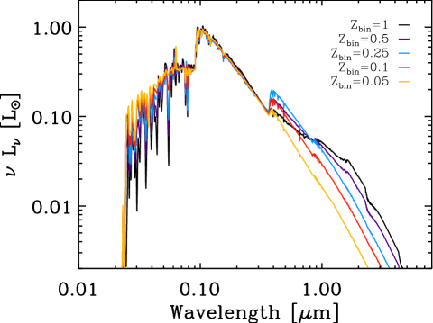
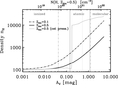
The source of radiation is chosen as a young starburst that we simulated with Starburst99 (Leitherer et al., 2010). We opted for a continuous star formation spectral energy distribution (SED) computed out to an age of 10 Myr. The stars were selected from the standard Geneva tracks (without rotation) and distributed on a Kroupa IMF (slope between 0.1 and 0.5 and between 0.5 and 100 ; Kroupa 2001). The Starburst99 spectra are shown in Figure 1 for the different values. We also added a small soft X-ray component (blackbody peaking at 1.5 keV) to the input radiation field and adopt a cosmic ray rate of s-1 (see Section 5.2.2 for a justification of those parameters). We adopted a density profile that is roughly constant in the H ii region and increases linearly with the hydrogen column density in the neutral gas (see Fig. 2, and Table 2).This density profile is an intermediate choice between the more extreme, common assumptions of a constant density or of constant pressure (that we test in Section 5). In the following, unless stated otherwise, refers to the initial density. It is the density in the H ii region. All models were stopped at an of 5 mag to ensure going deep enough in the cloud for complete PDR predictions. We note that this corresponds to different values for different values. Stopping the models at a fixed value instead of a fixed value would not change our results as long as is chosen large enough so that the PDR lines ([C ii], [O i]) are fully produced. The transitions from the ionized to the atomic and from the atomic to the molecular regions are defined where the fractions of and H0, and H0 and H2 respectively, are equal to 0.5. We note that in environments with high ionization parameters, radiation pressure could become dynamically important if it dominates the other pressure terms. This could be considered an unstable model. For our models, we have verified that this is not the case.
We generated a grid of models for each of the five metallicity bins by varying the following parameters: the initial density () from to cm-3, and the inner radius such that we cover an ionization parameter () from to . Values of and are those at the start of the calculation. Since the PDR conditions are set by the H ii region model (by continuity), there is little degree of freedom on the PDR parameters. The radiation field is set by that in the H ii region and the density is set by the adopted density profile. As a free parameter we chose the covering of the PDR with respect to the H ii region which always has a covering factor of unity. The PDR covering factor () is not varied within the grid but a posteriori, from zero to unity, because it just corresponds to a linear scaling of the PDR intensities. We note that with this setup, the H ii region is always radiation bounded, in other words no ionizing radiation escapes. In the case of a low PDR covering factor, segments of the H ii region that are not covered by neutral gas could be stopped at lower , before the ionization front is reached (making the model matter bounded with ionizing radiation escaping). However, this stopping parameter can only be constrained by specific lines tracing the ionization front (e.g., [Ar ii], [Ne ii]), and it introduces degeneracies with other parameters (see Polles et al., 2019, for a detailed analysis with this method). Hence we prefer not to add an additional free parameter and to keep all models radiation bounded. For the following discussion, we use the term porosity when referring to a reduced covering factor of the dense neutral gas (PDR) relative to the ionized gas as determined by the modeling. For convenience, we have provided line luminosities from the grid of models predicted at the ionization front and at an of 5 mag as online material.
Most of the choices for the model parameters described above are motivated by observations or set to default values. However, uncertainties in those choices can remain. In Section 5, we change some of the input parameters (namely the radiation field, the presence of cosmic rays and X-rays, the turbulent velocity, the density law, and the dust abundance) and we discuss their influence on the results.
| Fixed parameters | |
|---|---|
| Radiation field | Starburst99 continuous SF of 10 Myr, |
| … Geneva stellar track, scaled to , | |
| … Kroupa IMF, | |
| … log() = 9 | |
| blackbody K (X-ray), | |
| … log() = 5.2 | |
| cosmic rays background 0.5 log | |
| CMB | |
| table ISM | |
| 1.5 km s-1 | |
| mass ratio | |
| metal, PAH abund. | set to values below |
| density law | |
| stopping criterion | = 5 mag |
| Varied parameters and grid values | |
| [0.5, 1.0, 1.5, 2.0, 2.5, 3.0, 3.5] cm-3 | |
| [-4, -3.5, -3, -2.5, -2, -1.5, -1, -0.5] | |
| [0, 0.2, 0.4, 0.6, 0.8, 1] | |
| [ 0.05, 0.10, 0.25, 0.50, 1.00] | |
| [, , , , ] | |
| [, , , , ] | |
| [, , , , ] | |
| [, , , , ] | |
| [, , , , ] | |
| [, , , , ] | |
| [, , , , ] | |
| [, , , , ] | |
| [, , , , ] | |
| [, , , , ] | |
3.2 Comparison to observations
3.2.1 Observed and adopted model abundances
Elemental abundances have been measured from optical spectroscopy in several of our galaxies. Their values are reported in Table 6 in the appendix. Oxygen abundances are estimated with the Pilyugin & Thuan (2005) calibration. We refer the reader to Rémy-Ruyer et al. (2014) for further details and references on abundances and to Madden et al. (2013); De Vis et al. (2017) for a comparison of metallicities obtained with other methods in the DGS galaxies. Since abundances in the model grid are fixed, a correction needs to be applied when comparing models to observations of a given galaxy. For small abundance variations, abundances, and intensities scale linearly. For each galaxy, we select the grid of models with metallicity (oxygen abundance) closest to the observed value (tabulated in Tables 3 and 4 as ). Then, for elements with measured abundances, we multiplied the predicted line intensities by the offset between the observed abundances (Table 6) and the adopted model abundances (Table 2). For example, for a galaxy with , we select the grid in the metallicity bin and multiply the oxygen line intensities by . Oxygen abundances are measured for all of our galaxies. For the other elements, if not measured, their abundances are still assumed to follow the patterns in Table 2, hence we interpolate values in that table considering the observed value. The abundance values quoted here can be uncertain and vary within galaxies or according to the datasets and methods used to measure them. For our galaxies, literature studies indicate that those variations are on the order of 0.2 dex. We see similar offsets between the measured abundances and the abundance patterns adopted in Table 2. Hence we took into account an uncertainty from abundances that we set to 50% of the observed line intensities.
3.2.2 Observed and modeled luminosities
To compare the absolute fluxes observed to model predictions, we needed to scale the luminosity of the model to that of the source. We calculated a nominal scaling factor as the ratio of the average observed luminosity to the average predicted luminosity of the main ionic lines to fit. In addition to reproducing the line luminosities, the successful scaled model should also reproduce the continuum luminosity () because this corresponds to the amount of stellar light reprocessed by dust in the PDR. Contrary to which is used as a formal constraint on the models, the bolometric luminosity of the galaxies () is not used as a direct constraint. In principle, the input luminosity of the models should be equal to the bolometric luminosity. However, the correct value of the input luminosity in case of partial PDR coverage is difficult to assess. By energy conservation, the input luminosity of the models must be equal to (if ) or greater than (in case of escaping photons, ). It should be, at most, the bolometric luminosity of the galaxy (i.e., all energy is associated with the model stellar cluster). is compared a posteriori to the input luminosity of the models to identify large mismatches that could, for example, indicate sources of heating other than stars. We identify a limited number of such cases (see Section 4.4.2).
3.2.3 Goodness of fit
We searched for the best-fitting models by minimizing the defined as
| (1) |
where and are the modeled and observed intensities, and is the fractional error on the observed flux (uncertainty/flux) with calibration and abundance uncertainties added in quadrature to the measured uncertainties. A line is considered not detected when its flux is lower than three times its measured uncertainty. For non-detections with a 1 upper limit , we set to if (i.e., no contribution of the upper limit to the ) and we set to and to 1 if . The number of free parameters in the models is three (density, ionization parameter, and PDR covering factor). The reduced is given by where is the difference between the number of constraints and the number of free parameters.
3.2.4 Reliability of the derived physical parameters
The minimization gives an idea on the models that are closest to the observations. However, it is possible that those models do not converge to a single value of the free parameters that we aim to constrain. To assess how well the free physical parameters are constrained, we compute their probability distribution functions (PDFs). The marginalized PDF of a given parameter is calculated at each fixed value of this parameter. It is taken as the sum of the probabilities () of all the models having this parameter set to its fixed value and all possible values for the other parameters. The PDFs are then normalized such that the sum of probabilities of all models in the grid is equal to one. We estimated uncertainties on the best-fit parameters by considering the average and standard deviation of the values of the free parameters taken by models with values within a certain range of . For instance, for a number of degrees of freedom of four, and a 1 confidence level (probability of 68.3%), this range is (Press et al., 1992).
4 Results
We present general grid results in Section 4.1 and results from fitting the grid models to the observations in the following subsections.
4.1 Grid results
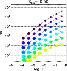
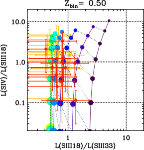
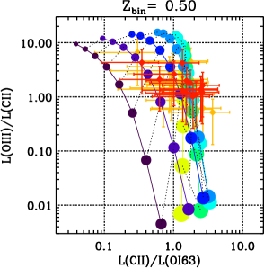
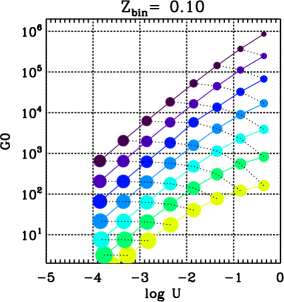
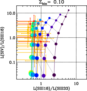
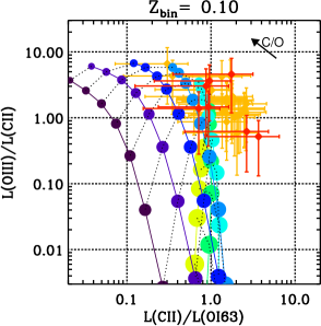
Figure 3 shows the parameter space covered by the models and the observations for and . In the left panels, we see the values of produced when varying the ionization parameter and the density, which are input parameters of the model grid. We remind the reader that is the intensity of the ultraviolet radiation field at the PDR front, given in units of the background Habing (1968) value, erg cm-2 s-1, as defined by Tielens & Hollenbach (1985). For a given density, and scale linearly (except at the high-, low- end due to geometric dilution of the field; see e.g., Cormier et al. 2015). The middle panels of Fig. 3 show diagnostics of the H ii region. The [S iii] line ratio traces intermediate densities ( cm-3), independently of . Model predictions for the [S iv]/[S iii] line ratio are slightly shifted up at compared to , especially for low- values, because the starlight radiation field is harder. Observations span values between and for the [S iv]10/[S iii]18 line ratio and between and for the [S iii]18/[S iii]33 line ratio. Both grids at and cover the observations quite well. Observations are rather compatible with models of low/ intermediate-densities and high- values. The right panels of Fig. 3 show a diagnostic linking the H ii region and the PDR. We see that predictions of the [O iii]/[C ii] and [C ii]/[O i] ratios vary significantly with . The main effects at work are the C/O abundance ratio that decreases by a factor of two from to , the harder stellar radiation field at making more [O iii], and the fact that the PDR structure is very sensitive to . In particular, with decreasing , the PDR lines are formed up to a larger column density and their emission is boosted relative to the ionized gas metal lines (i.e., predictions going down in Fig. 3, right panels). Observations span values between and for the [O iii]88/[C ii]157 line ratio and between and for the [C ii]157/[O i]63 line ratio. At , models cover quite well the observed ranges, while at , we notice that model predictions are at the edge of the observed ratio ranges. This suggests that a combination of models and/or low covering factor of the PDR may be needed to match better the observations.
We remind the reader that normal, star-forming, metal-rich galaxies have similar [S iii]18/[S iii]33 and [C ii]157/[O i]63 ratio values than the DGS galaxies, but their [S iv]10/[S iii]18 and [O iii]88/[C ii]157 values are respectively about seven times and four times lower (Brauher et al., 2008; Dale et al., 2009; Cormier et al., 2015). Those values are covered by our grid of models and compatible with models of low or intermediate-densities and intermediate- values (for ).

4.2 Best-fitting single H ii +PDR models
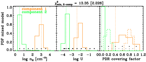
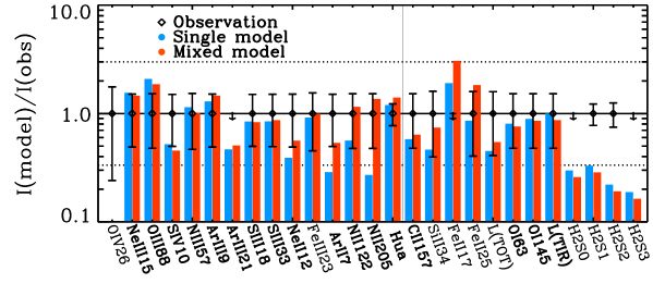
Parameters of the best-fitting single models as well as their corresponding and reduced () are indicated in Tables 3 and 4. The number of detected lines in each galaxy varies from three (model under-constrained) to . Figure 4 shows how the observed and predicted line intensities compare for the best-fitting model of He 2-10, as well as the PDFs of , , and . Figures for the other galaxies of the sample are shown in Appendix D. The ionization parameters vary between and with median value , and the PDR covering factor varies from 0.2 to one with a median value of 0.4. Densities of the best-fitting models vary from to cm-3, with median at cm-3. The medians are very close to the values and cm-3 found in Cormier et al. (2015) from average line ratios of the DGS sample. The classical MIR density tracers ([S iii] and [Ar iii] line ratios) are not particularly sensitive to those low densities, and although we can recover such densities by modeling a suite of lines, future determinations of electron densities in dwarf galaxies would benefit from FIR observations of line doublets such as the [O iii]52 and [O iii]88 or [N ii]122 and [N ii]205 lines.
About half of the galaxies (16/39) have minimum below two and their observed lines are satisfyingly reproduced by a single model. Inspection of the results indicates that galaxies with larger usually have one or more lines for which predictions are off by a factor of more than two. The lines that are most difficult to reproduce simultaneously with the other lines are [S iv] and [Ne ii].
| 1-component model | 2-component model | ||||||||||||
|---|---|---|---|---|---|---|---|---|---|---|---|---|---|
| Galaxy | log | log | log | log | log | log | |||||||
| NGC1705 | 0.50 | 8 | |||||||||||
| IIZw40 | 0.50 | 13 | |||||||||||
| Mrk930 | 0.25 | 12 | |||||||||||
| NGC1569 | 0.25 | 13 | |||||||||||
| HS1330 | 0.25 | 5 | |||||||||||
| HS1304 | 0.25 | 5 | |||||||||||
| Mrk153 | 0.25 | 9 | |||||||||||
| UM133 | 0.25 | 4 | |||||||||||
| HS1319 | 0.25 | 3 | |||||||||||
| HS1222 | 0.25 | 4 | |||||||||||
| Mrk209 | 0.10 | 8 | |||||||||||
| Pox186 | 0.10 | 7 | |||||||||||
| SBS1249 | 0.10 | 4 | |||||||||||
| HS0017 | 0.10 | 3 | |||||||||||
| HS1442 | 0.10 | 4 | |||||||||||
| SBS1211 | 0.10 | 5 | |||||||||||
| SBS1415 | 0.10 | 8 | |||||||||||
| Tol1214 | 0.10 | 6 | |||||||||||
| UGC4483 | 0.10 | 4 | |||||||||||
| SBS1159 | 0.10 | 6 | |||||||||||
| HS0822 | 0.05 | 5 | |||||||||||
| SBS0335 | 0.05 | 9 | |||||||||||
| IZw18 | 0.05 | 8 | |||||||||||
| 1-component model | 2-component model | ||||||||||||
|---|---|---|---|---|---|---|---|---|---|---|---|---|---|
| Galaxy | log | log | log | log | log | log | |||||||
| He2-10 | 1.00 | 16∗∗ | |||||||||||
| NGC1140 | 1.00 | 13∗ | |||||||||||
| NGC4214-s(e) | 0.50 | 11∗ | |||||||||||
| Haro11 | 0.50 | 16∗∗ | |||||||||||
| UM448 | 0.50 | 14∗ | |||||||||||
| Haro3 | 0.50 | 14∗ | |||||||||||
| NGC5253 | 0.50 | 14∗ | |||||||||||
| Haro2 | 0.50 | 10 | |||||||||||
| NGC625 | 0.50 | 11 | |||||||||||
| NGC4214-c(e) | 0.50 | 12∗∗ | |||||||||||
| Mrk1089 | 0.50 | 13∗ | |||||||||||
| HS0052 | 0.25 | 9 | |||||||||||
| SBS1533 | 0.25 | 9 | |||||||||||
| Mrk1450 | 0.25 | 11∗ | |||||||||||
| UM461 | 0.10 | 9 | |||||||||||
| VIIZw403 | 0.10 | 9 | |||||||||||
4.3 Mixing two model components
4.3.1 Motivation
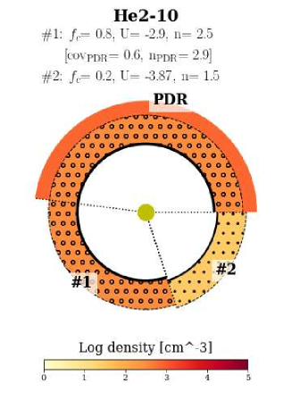
It is possible that the minimum for single models as described above does not provide a satisfying fit to the data because our model description is too simple. In addition to single models, we explored the possibility of mixing two models of the grids: one dense high- model (model #1), which should represent the material that gave birth to the starburst, and one more diffuse lower- model (model #2), which should represent a hypothetical more extended ionized phase. This two-component modeling approach is supported by earlier work on those DGS galaxies suggestive of a large filling factor, diffuse, ionized gas phase (Cormier et al., 2012, 2015; Dimaratos et al., 2015). For this, we have generated a new set of models by combining two models for which parameters are varied within the parameter space of our original grid, and their relative contribution (in terms of luminosity) varies from 10% to 90% in steps of 10%. That is, for a given line, the intensity prediction of the combined model is the sum of the prediction of the first model multiplied by and of the prediction of the second model times . Given the small number of constraints for the PDR, we consider that only the dense H ii model produces a PDR. In that case, we have as free parameters for the mixed models: (but ), (but ), and (with ). The number of free parameters is five. Figure 5 shows an illustration of the best-fitting model for one example galaxy and figures for each galaxy of the sample can be found in Appendix B. We stress that for mixed models, and are different quantities. corresponds to the contribution of a given model to the final (2-component) model, it is therefore translated into a covering factor of the H ii region in Fig. 5. is the covering factor of the PDR relative to that of the H ii region, hence the covering factor of the final model is .
For galaxies with fewer than six lines detected (for which a mixed model would be under-constrained) or with from the single models lower than two (or lower than with the mixed models), we consider the single best-fit model to be the best representation. There are galaxies that satisfy this condition (results reported in Table 3). For the other galaxies, we consider the mixed best-fit model to be better (results reported in Table 4).
(a)
 (b)
(b)

(c)


4.3.2 Results for mixed models
In order to reproduce all observed line intensities in galaxies where a single model fails (), we search for a combination of two model components. We stress that the second component is not added to the single model but a new set of two model components is found (with some constraints on those parameters as explained in the previous subsection). Parameters of the best-fitting mixed models as well as their corresponding are indicated in Tables 3 and 4. Similar figures as for the single model case are shown in Fig. 4 and in Appendix D for all galaxies.
In general, the lines that were not satisfyingly reproduced with single models are well fit by mixed models. The low- component contributes mostly to the [N ii], [Ne ii], [Ar ii], and [S iii] lines. We note that the two -values of the mixed models always bracket the -value of the single models, while the -values of the mixed models are sometimes lower than the -value of the single models (for example, NGC 625, SBS 1533). For those galaxies, the single models tend to under-predict the [C ii]157/[O i]63 ratio by a factor of two to three while the lower -values of the mixed models reproduce this ratio better. Overall, our observations seem to be more sensitive to variations in the ionization parameter, although there might be also some degeneracy at play between density and covering factor for the PDR lines. The PDFs of the parameters of the mixed models are sometimes broader than for the single models, especially for the lower-density component, indicating that it is not very well constrained by the observations. In most cases, the denser component contributes more than the lower-density component to the final mixed model ().
For most galaxies for which single models do not provide a good fit, the mixed models perform better (lower ). All galaxies for which mixed models are preferred have . For several galaxies though, mixed models do not improve the results over the single models but provide similar (II Zw 40, Mrk 209, Pox 186, SBS 0335, SBS 1159, SBS 1415) or worse (Tol 1214). For two of them (SBS 1159, Tol 1214), remains above three. For those two galaxies, we find that the combination of a low-, high- component going in the PDR and a high-, low- component would actually fit the data better (with close to unity). For the galaxies where a single model was already giving a good fit, the mixed models provide lower but are often under-constrained. The parameters of the two model components are sometimes very similar to the parameters of the single model or they bracket them (especially for and less so for , as noted above).
Comparison to previous, similar studies:
At this stage, it is worth comparing our findings to
two previous studies that we carried out to model
MIR and FIR lines using a similar approach.
Results for Haro 11 are in global agreement with previous
modeling done in Cormier et al. (2012). For the H ii region,
we find similar densities ( cm-3 and cm-3 versus cm-3 and cm-3 here). The
-values are somewhat different ( and
versus and ). This is mainly driven by
the different stellar spectra used in input (instantaneous
burst and single star versus continuous star-formation
scenario here). For the PDR, we find a larger PDR
covering factor because the PDR density is lower
than in Cormier et al. (2012) where the density was set by
pressure equilibrium between the H ii region and the PDR.
For the two star-forming regions of NGC 4214, we also find
very similar results for single models to Dimaratos et al. (2015),
with lower density, ionization parameter, and PDR covering
factor in the central region compared to the southern region.
Mixed models (not included in Dimaratos et al. 2015) are
however better suited to reproduce the [N ii] emission in NGC 4214.
4.4 A posteriori checks
4.4.1 Mid-infrared lines
We have not used the silicon, iron, and H2 lines from the Spitzer IRS instrument to constrain the models due to the ambiguous origin (possibly shocks) of those lines and uncertain gas-phase abundances. However, we have compared predictions from the best models a posteriori. We report on the performance of the single and mixed models in predicting those secondary lines in Table 5.
| Line | Single models | Mixed models | |
|---|---|---|---|
| low — ok — high | low — ok — high | ||
| [Si ii] 34.82 | |||
| [Fe ii] 17.94 | |||
| [Fe ii] 25.99 | |||
| [Fe iii] 22.93 | |||
| H2 S(0) 28.21 | |||
| H2 S(1) 17.03 | |||
| H2 S(2) 12.28 | |||
| H2 S(3) 9.66 | |||
The [Si ii] line at 34 m can originate in the ionized gas and in the neutral ISM. It is quite bright and detected in many of the galaxies of our sample. We find that the [Si ii] line is systematically under-predicted by a factor of two to six by the best-fitting models. Mixed models perform slightly better than single models although [Si ii] remains under-predicted in most cases. Since our models include the H ii region and a diffuse, low-excitation ionized phase in the case of mixed models, any contribution of ionized gas to [Si ii] emission is largely taken into account by our models. Thus, reasons for the under-prediction of [Si ii] could be additional excitation of [Si ii] by shocks or uncertainty in the adopted gaseous abundances. Given the difficulty in modeling iron (see below), we cannot really compare our results for [Si ii] with those for [Fe ii] to rule out shock excitation.
The mid-infrared iron lines are faint and detected in only a few galaxies of our sample. The [Fe ii] line at 25.99 m is generally well reproduced while the [Fe iii] line at 22.93 m is over-predicted by a factor of two to three for half of the sources with detection, even when adding those lines in the list of lines to fit for. We note that collisional excitation of [Fe ii] by H and H2 is not included in the version of Cloudy used in this work, hence an additional contribution from PDRs to the [Fe ii] emission (not included in our models) would then over-predict the observations. However, the main effect affecting the line prediction is again the adopted abundances. Although measured for many of our galaxies (Table 6), abundances can be uncertain because of unknown ionization corrections, depletion of iron in the cold dense medium (Savage & Sembach, 1996), or enhancement of iron from supernovae-driven shocks (O’Halloran et al., 2008). In our case, adopted abundances may be systematically too high. At solar metallicity, Kaufman et al. (2006) consider an iron abundance ten times lower than our adopted abundance.
The H2 rotational lines are also faint and detected in few galaxies in our sample. The S(1) transition at 17.03 m is sometimes over-predicted and sometimes under-predicted by a factor of two to fifteen, while the S(2) transition at 12.28 m is usually under-predicted by a factor of three to ten. The ratio of those two transitions is mostly sensitive to density for (Kaufman et al., 2006). When fitting for the H2 lines, the densities required for the PDR are indeed larger (typically cm-3 at the PDR front) but increases a lot (models performing worse for some H ii lines, [C ii], [O i]). More H2 detections are required to really investigate the presence and importance of shocks.
4.4.2 Bolometric luminosity
As explained in Section 3.2.2, the total luminosity of the models is not an easy parameter to constrain. Here we just verify that the total luminosity of the best-fitting models does not exceed the observed bolometric luminosities. Table 5 shows that this condition is satisfied for all galaxies in the case of single models. In the case of mixed models, for galaxies, the luminosity required by the models is larger than the observed by a factor of three to four in most cases and up to for one galaxy. For all those galaxies, the diffuse ionized component contributes to the majority of the total luminosity, and for ten of those galaxies, the single models are actually preferred. For the two galaxies where mixed models are preferred (HS 0052 and Mrk 1089), is over-predicted by a factor of three. When interpreting this over-prediction, one should not forget that there is a range of acceptable values for each model parameter (PDFs in Fig. 4 and in Appendix D). Indeed, a density of cm-3 (value often within the acceptable range) instead of cm-3 for the diffuse component of those two galaxies would reconcile better the total observed and modeled luminosities. We also note that we calculated the observed bolometric luminosity relatively coarsely.
4.4.3 Optical lines
Since the optical lines are very sensitive to extinction and to the distribution of dust in the models, as opposed to the infrared lines, and their observations often cover a smaller field-of-view, we do not include them in finding the best-fitting models. A posteriori comparisons indicate that the intensity ratios of the optical lines relative to H are generally well reproduced by the models (within a factor of three). To assess how the best-fitting models would perform for the total fluxes (i.e., not normalized to H), we also compare the ratio of total observed H luminosity (references in Rémy-Ruyer et al. (2015), mainly from Gil de Paz et al. (2003)) to the [O iii]88 luminosity. We find that the observed H/[O iii]88 ratio is matched by the models (within a factor of two) for more than half of the galaxies of the sample, and it is over-predicted for the other galaxies by a factor of three to eight. The discrepancies with optical observations are likely caused by extinction/geometry considerations and reproducing them, simultaneously with IR lines, is not trivial (and neither is it the goal of this study; see also Polles et al. 2019).
4.5 Contributions to the [C ii] and [Si ii] emission
The use of the [C ii] line at 157 m as a reliable neutral gas/PDR tracer has been questioned since it can also originate from diffuse ( cm-3), low-excitation ionized gas. To quantify such contribution to the observed [C ii] intensity, it is often compared to the [N ii] lines at 122 m or 205 m, which have low ionization potentials and low critical densities. In metal-rich environments, the fraction of [C ii] emission arising in the H ii region ranges from 5% to 60% (e.g., Malhotra et al., 2001; Pineda et al., 2013; Parkin et al., 2014; Hughes et al., 2015; Abdullah et al., 2017; Croxall et al., 2017; Díaz-Santos et al., 2017; Lapham et al., 2017). The low [N ii]122/[C ii]157 values measured in the dwarfs (Cormier et al., 2015) suggest little contribution of the H ii region to the observed C+ emission. Similarly, [Si ii] can arise from low-excitation ionized gas but it has higher critical density with electrons than [C ii] ( cm-3). The H ii region produces significant [Si ii] emission, more than the PDR, at moderate densities and low- (see also Abel et al., 2005). With the physical conditions constrained in most of the DGS galaxies, we can quantify more precisely how much [C ii] and [Si ii] emission is predicted to arise from the ionized gas. The definition that we use to measure this is to take the intensity predictions at the phase transition from ionized to atomic gas (i.e., where the fractions of and H0 are equal to 0.5).
In the case of single models, we find that the fractions of [C ii] and [Si ii] predicted in the H ii region are small, typically less than 10% for [C ii] and less than 40% for [Si ii]. In the case of mixed models, those fractions generally increase slightly but remain below 40% for [C ii] and 50% for [Si ii]. Regardless of density, it is the low- component which contributes most to those fractions. The fractions of [C ii] and [Si ii] emission from the ionized gas are generally low in the single models because most ionic lines that we observed or detected require high- values. A possible additional low- component will increase these fractions but the parameters of this component can only be constrained when [N ii] and, to a lesser extent, [Ne ii] and [Ar ii] are available. We further discuss the fractions of [C ii] from the ionized gas with other galaxy parameters and line diagnostics in Section 6.1.
5 Influence of some modeling choices
In the methodology described in Section 3, we have made choices regarding the set of spectral lines to fit as well as the set of model parameters to fix or vary. Not all of the input parameters can be varied and fit by our observations. We have taken care to use the best input fixed parameters and the motivation of their choices for several of them is given below. In this section, we further explore: 1) how the inclusion or exclusion of specific lines can change the best-fitting results (Section 5.1); and 2) the influence of varying one of the fixed parameters at a time (Sections 5.2 to 5.5). For 2), we focus on the metallicity bins and , and we make comparison to galaxies in those bins (including Haro 11 which we study in detail in Cormier et al. 2012).
5.1 Set of spectral lines to fit
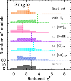
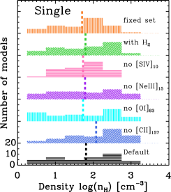
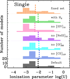
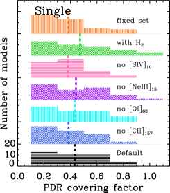
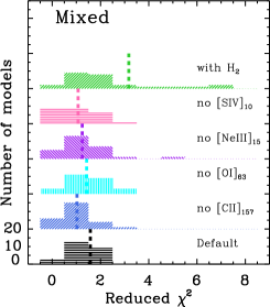
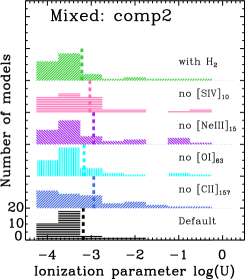
As discussed in the previous section, spectral lines that are known to be problematic for the adopted modeling strategy were excluded from the fit (for instance if shock heating or geometry effects can be important). Now, within the default set of fitted lines, we aim to determine the effect of excluding some specific lines on the best-fitting results and to identify possible biases. For this, we have considered excluding, one at a time, the [C ii]157 line which can arise from more diffuse gas than [O i], the [O i]63 line which can be optically thick, the [Ne iii]15 line which can be problematic to model from population synthesis models (see Section 5.2), and the [S iv]10 line which is usually well detected but one of the lines that is least well reproduced by our models. We also consider including the H2 lines in the fit and fitting a small, fixed set of lines ([C ii]157, [O iii]88, [Ne iii]15, and ) since several of the low- galaxies are only detected in those lines.
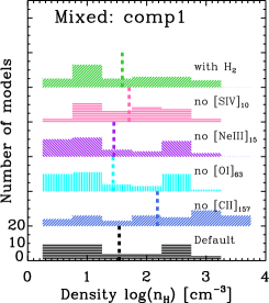
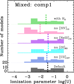
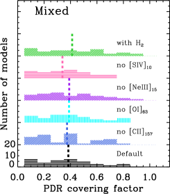
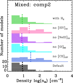
The results are shown in Figure 6. We plot histograms of the best-fitting parameters and values for both single and mixed models. We note that all galaxies are included and uncertainties on the best-fitting parameters as well as quality of the fits are not conveyed on the plots. For single models, seems to improve quite significantly when excluding [S iv]. For mixed models, the distributions of remain similar and the mean values are only slightly lower when excluding a specific line. Compared to the default case, the distribution of model parameters for the tests performed have relatively similar shapes, and individual galaxies typically move to the neighboring bin at most. Excluding [O i]63 or [Ne iii]15 does not have a significant impact on the best-fitting parameters, while the distribution of those parameters change noticeably when excluding [S iv] or [C ii]. Indeed, by excluding [S iv], there are fewer galaxies with best-fitting models that have very low density ( cm-3), hence the mean density of the mixed, low-density component is larger. The mean ionization parameters of the single and mixed, high-density components are also slightly lower, probably because [S iv] has one of the highest ionization potentials. Similarly, when considering the small, fixed set of fitted lines (which only allows for single models, not mixed models), the distribution of the best-fitting solutions does not change significantly but the uncertainties on the model parameters are larger. There are fewer galaxies at the highest densities, probably because the [S iii] lines are not available to constrain further the density and the mean ionization parameter is also slightly lower because [S iv] is excluded from the fit. We want to stress that the trends of best-fitting parameters with global galaxy properties (SFR, ) discussed in Section 6 persist with this test. By excluding [C ii], the distributions of densities shift to larger (factor of three on average) values and the distribution of PDR covering factors also shifts to slightly lower values. This can be understood as the PDR solution is driven by and the [O i] lines which generally trace the denser, lower filling factor regions of PDRs than [C ii]. Including the warm H2 lines in the fit does not affect the overall distributions and mean values of the model parameters because those lines are detected in only eight galaxies of our sample. Those lines are difficult to reproduce though, yielding larger values on average.
5.2 Choice of input radiation field
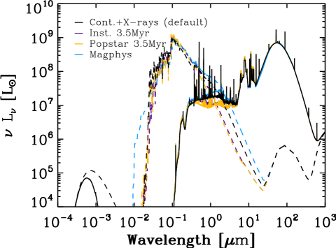
The sources of radiation giving rise to the observed line emission are multiple and mainly clustered in a few star-forming regions. Given the limited geometry of Cloudy, we consider only one central source per model and need to choose its radiation field. Several input SEDs were tested (Figure 7). In this section, we discuss the effects of different starburst spectra and heating by X-rays and cosmic rays on the line predictions and best-fitting models.
5.2.1 Starburst spectrum
We tried as input the Starburst99 stellar spectrum both from an instantaneous burst with an age between 3 and 6 Myr, and from a continuous (up to an age of 10 Myr) star-formation scenario. In the instantaneous case, we find that the emission of lines tracing the radiation field hardness is too sensitive to the step size for sampling the burst age, making it easy to miss the “best” age (see also Polles et al. 2019). It is also probably not the best representation of the cluster age distribution in galaxies. Moreover, the PDR lines are better fit with a continuous star-formation scenario, in part because is too high with an instantaneous burst (fewer lower-energy photons). We also tried an instantaneous burst using the Popstar evolutionary synthesis models (Mollá et al., 2009). A different treatment of the stellar atmosphere can produce significant differences in the stellar spectrum for photons with energy eV, hence affecting predictions of lines such as [Ne iii] (Morisset & Georgiev, 2009). However, similar problems persist, as noted above for the Starburst99 instantaneous case.
For a more complex star-formation scenario, we also tried to constrain the shape of the incident spectrum by taking the optical photometry into account. Focusing on Haro 11, we used the SED code Magphys (da Cunha et al., 2008) to obtain an unattenuated spectrum and used that spectrum as input in Cloudy. However, for the lines that we fit (H ii region and PDR) the results are not especially improved ( was not lower) than with the continuous scenario of Starburst99. Moreover, since the available optical photometry is limited for some of our galaxies, we cannot use Magphys for all galaxies of our sample. It is important to have a consistent method in order to study trends. Therefore, we opt for a continuous star-formation scenario for our grid of models.
5.2.2 Heating of the PDR and [O i] line ratio
The standard model contains a soft X-ray component of luminosity times the bolometric luminosity and cosmic rays. This is primarily needed for understanding the [O i] line emission. The [O i] 145 m line is clearly detected in galaxies and the [O i] 63 m line in galaxies of the sample, with [O i]145/[O i]63 luminosity ratios ranging from to (Cormier et al., 2015). The [O i] 63 m line is known to suffer from optical depth effects or self-absorption in regions of the Milky Way and dusty galaxies (e.g., Liseau et al., 2006; Abel et al., 2007; Rosenberg et al., 2015), giving rise to [O i] line ratios above . The emergent line ratio is somewhat sensitive to the depth () of the models (Abel et al., 2007). Other heating sources than the stellar radiation field can also affect the PDR chemistry and line emission, such as cosmic rays or X-ray or shock heating. We explored the effect of high column density (high ), cosmic rays, and soft X-ray heating in Figure 8.
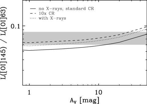
With no additional heating source than the stellar spectrum, the observed range of [O i] line ratios requires systematically high , at which the CO optical depths are also very large, and this seems unlikely. Indeed, the mean is expected to decrease with decreasing mean metallicity, and CO emission is known to be clumpy at low , suggesting that the [O i] emission integrated over entire galaxies is probably little affected by high- ( mag) sightlines.
Soft X-ray emission (0.2-2 keV) is detected in several galaxies of our sample, with an observed luminosity about times lower than (except in I Zw 18 which is strong in X-rays; see Lebouteiller et al. 2017). The intrinsic (unabsorbed) emission should be higher, however we do not know how much of that emission goes into the heating of the dense ISM (as opposed to diffuse isotropic emission). Hence we decide to add a soft X-ray component to the input radiation field of our models that we take as a blackbody spectrum of temperature K (to peak around 1 keV) and luminosity in the soft X-ray range . Adding the X-rays creates a hybrid XDR/PDR model in Cloudy. X-rays generally do not affect the predictions of the inner ionized gas cloud but increases the heating at the ionization front and in the PDR (e.g., Meijerink & Spaans, 2005; Lebouteiller et al., 2017). In the presence of strong X-ray flux, the deeper penetrating X-rays produce more Ne+ and Ar+, while the increased ionization has an effect on CO, suppressing its formation due to reactions with He+ and H (e.g., Meijerink & Spaans, 2005; Abel et al., 2009). This produces more free oxygen and a higher gas temperature. In our case, the X-ray component has low luminosity. The main effect is that the PDR temperature increases roughly from 150 K to 200 K. The emission of the PDR lines increases slightly, as well as the [Ne ii] and [Ar ii] emission for models with low-density or high-. In the case tested in Fig. 8, the predicted [O i] line ratios go up by a factor of .
Regarding the cosmic rays, we show in Fig. 8 the effect of increasing the standard cosmic ray rate ( s-1; Indriolo et al. 2007) by an order of magnitude. Similarly to the case with soft X-rays, the PDR heating and line emission are enhanced. The cosmic ray rate varies significantly from sightline to sightline in the Galactic ISM (e.g., Dalgarno, 2006; Neufeld & Wolfire, 2017), and the dwarfs of our survey have undergone recent star formation, hence it seems reasonable to adopt a different value than the standard rate. To match the observed [O i] line ratios, we decided to increase the cosmic ray rate by a factor of three.
We note that cosmic rays and X-rays have similar effects (ionization and heating) and distinguishing between the two with no other constraints is not possible. One way to constrain the cosmic ray flux would be to study its effect on the ionization and coupling of the magnetic field and the gas in the PDR (Padovani & Galli, 2011).
5.3 Turbulent velocity
The micro-turbulent velocity affects the shielding and pumping of lines. It is included as a pressure term in the equation of state. Hence, we expect that it impacts mainly predictions of PDR and high optical depth lines. We set the turbulent velocity to 1.5 km s-1 in the default grid of models, as in Kaufman et al. (1999), and here, we explored the cases km s-1 and km s-1 for the grid of models in the metallicity bin . We find that, by increasing the turbulent velocity from 0 km s-1 to 5 km s-1, the PDR temperature reduces marginally by about 10%, the [O i] line intensities are down by 15%, the [C ii] intensity is up by 20%, and the H2 lines are down by 30%. Overall, the turbulent velocity does not have a significant impact on our resulting best-fitting models and therefore on our trend analysis.
5.4 Density law
One of the model choices with the largest consequence is the density profile to adopt. As default, we adopted a density profile that increases smoothly with depth (see also Hosokawa & Inutsuka, 2005; Wolfire et al., 2010). Here we have tested, for the grid of models in the metallicity bin , two other often-used options: a constant density throughout the H ii region and the PDR, and hydrostatic equilibrium. Hydrostatic equilibrium assumes that the total pressure (including gas, turbulent, radiation pressure terms) is constant and implies a jump in density at the transition between the H ii region and the PDR (of almost two orders of magnitude when gas pressure dominates, see Fig. 2). The adopted density law affects mostly the PDR predictions with the constant density models predicting less [O i] emission and the constant pressure models predicting more [O i] emission than the default grid. For Haro 11, the dense component of the mixed model prefers higher initial densities in constant density and lower initial densities in constant pressure. However, we have tested the constant density and constant pressure hypotheses on eight other galaxies at (Haro 2, Haro 3, II Zw 40, Mrk 1089, NGC 625, NGC 1705, NGC 5253, UM 448), and those trends are not systematic. In general, we find that the constant density/pressure single models do not provide better fits to the observations. With mixed models, the constant pressure case provides (very marginally) lower than the default grid for eight of those nine galaxies. Overall, the smoothly increasing density law (adopted as default) is a reasonable choice for single models. It also provides satisfying fits for mixed models, although constant pressure models could also be considered but there is no clear evidence for the need to switch to constant pressure.
5.5 Abundance of PAHs and grains
Grains and PAHs are important for the energy balance, in particular for the cooling of the neutral ISM and heating via the photoelectric effect. The adopted abundances of grains and PAHs are motivated by recent analysis of the Spitzer and Herschel data (Rémy-Ruyer et al., 2014, 2015). However, there is both large scatter at all metallicities investigated () and a limited number of observations at . For example, the relation linking the DGR with metallicity seems to become steeper at than the relation calibrated on galaxies (e.g., Rémy-Ruyer et al., 2014). Concerning the PAHs, their abundance in the PDRs of dwarf galaxies is very uncertain as they are scarcely detected for with the Spitzer IRS instrument and we expect a large variation of the PAH-to-dust ratio between H ii regions and PDRs. We note that, if dust is present in the ionized gas but PAHs are weak there, a lower PDR covering factor at low (see Section 6.3) would significantly influence the globally observed PAH-to-dust emission ratios. Constraints on PAHs from the James Webb Space Telescope (JWST) will be very valuable. Departure from the default values and thus the effect on the results will be larger at low . Hence we carried out two tests for (and not as in the previous subsections): we adopt a PAH abundance lower; we adopt a DGR lower than in Table 2.
Results for the galaxies Mrk 209, Pox 186, SBS 1159, SBS 1415, Tol 1214, UM 461, VII Zw 403 (all at ) are inspected. Test does not change any of the results, probably because the PAH abundance was already low by default hence the PAHs contribute very little to the energy balance of those galaxies. Dust grains are responsible for the heating. Test affects the energy balance noticeably. By reducing the DGR by a factor of ten and therefore the dust grain abundance, the photoelectric effect remains the main heating source in the PDR but it is less important, and the PDR temperature goes down from K to 80 K. The cloud is also more transparent and the stopping criterion of of 5 mag corresponds to a larger depth. The emission of the [C ii] and [O i] lines increases by a factor of and , respectively. This grid with lower DGR at still does not cover the highest observed [C ii]/[O i]63 ratios (lower, right panel of Fig. 3. We find that the values are lower, especially for SBS 1159 and Tol 1214, and marginally for three other galaxies. The best-fitting models have slightly higher densities for four of the seven galaxies in this metallicity bin, but the best-fitting solutions do not change much and there are no clear systematic trends for all galaxies (in particular for the PDR covering factor which is discussed later).
In conclusion, we find that additional heating sources are not required to reproduce the PDR emission, as opposed to what was found by Lebouteiller et al. (2017) for I Zw 18, where X-rays are mainly responsible for the PDR heating and not grains. For this particular galaxy, our adopted DGR of might be too high since Lebouteiller et al. (2017) adopt a value of . We also conclude that the abundance of PAHs is not an important parameter for the models (as long as the dust grain abundance is larger). The dust grain abundance (and DGR) does, however, change the temperature structure of the cloud. For our study, this does not have a noticeable impact on the results, but additional PDR observations (such as MIR H2 lines for which line ratios are expected to change) and better constraints on the DGR would be needed for a more thorough study of the PDR properties.
6 Discussion
6.1 Origin of [C ii] emission
All of the ionic lines used in this study have critical densities for collisions with electrons larger than that of C+, making it difficult to constrain a low-density, low-excitation ionized phase from which [C ii] emission could arise. Optical lines such as [S ii] are often used as density tracers, but they probe a similar range of densities as [S iii], i.e., 100 to 10,000 cm-3, as well as shocks (Osterbrock & Ferland, 2006). [N ii]122 is the best line that we have in hand but, in principle, [N ii]205 is better suited (see Table 1 for critical densities). Croxall et al. (2017) and Díaz-Santos et al. (2017) carried out studies on the origin of [C ii] emission in nearby late-type spiral and luminous galaxies based on [N ii]122 and [N ii]205. In those galaxies, [N ii] line ratios that are indicative of electron densities between 1 and 300 cm-3 with median values at 30 and 41 cm-3, (Herrera-Camus et al. 2016 and Díaz-Santos et al. 2017, respectively; see also Herrera-Camus et al. 2018a).
Because of the issue of constraining the low-density ionized gas, it is interesting to compare our results on densities and fractions of [C ii] emission from the ionized gas with those obtained from theoretical calculations based on the [N ii] lines. We have also explored the sensitivity of those parameters to a fixed-density ionized gas component in the models.
-
•
Inferred electron densities from the [N ii] line ratio only:
[N ii]122 is observed in seven of our galaxies and [N ii]205 in only three of our galaxies: Haro 11, He 2-10, and NGC 4214-c. The [N ii]205/[N ii]122 ratios are observed to be , , and , respectively and are matched by models with densities between and cm-3. -
•
Comparison of observed [N ii] emission with models:
The single models often tend to under-predict [N ii]122 while the mixed models match [N ii]122 observations better. In Haro 11, He 2-10, and NGC 4214-c, we also fit for the [N ii]205 line and the best mixed models reproduce successfully both [N ii] lines, which emission arises from the low- (), low-density component ( of , and cm-3, respectively, values close to those inferred from the [N ii] line ratio only). -
•
Forcing a low-density component in the models:
For galaxies without [N ii] observations, we still would like to estimate how much [C ii] emission could arise from such low-density, low-excitation ionized phase. Here, we assume cm-3. We derived the fraction of ionized [C ii] by forcing the single models or one component in our mixed models to have a density of 30 cm-3 and an ionization parameter lower than that of the other component.
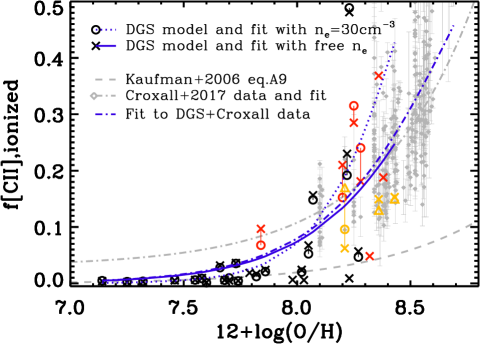
The results on the [C ii] emission arising from the ionized gas are presented in Figure 9. For the three galaxies with [N ii]205 detected, we first estimated the fraction of [C ii] emission from the ionized gas from theoretical calculations, based on statistical equilibrium of collisionally excited gas (see, e.g., Oberst et al. 2006 and Croxall et al. 2017). Those fractions range from % to % (triangles in Fig. 9) and are close to those derived from our models (circles and crosses in Fig. 9), though on the high side for NGC 4214-c. For all galaxies, we then compared estimates from our models with free and with fixed, low . In all cases, we find that the fraction of [C ii] emission coming from the ionized phase is at most 50%. In galaxies where [N ii] is observed, the models predict lower fractions of [C ii] in the ionized phase than predictions from Croxall et al. (2017) because our observed [N ii]/[C ii] ratios are on the low side of most of their observations. Predictions based on assuming a fixed low-density component ( cm-3) can be unreliable because they sometimes yield much higher than when is let free. Those predictions are not plotted in Fig. 9 if they yield . Based on our models, we also see a trend of decreasing fraction of [C ii] emission arising in the ionized gas with decreasing . The trend is similar to that reported by Croxall et al. (2017) and extends to lower values. For , our observations agree better with predictions from Kaufman et al. (2006) (their equation A9 for a low-density medium) than with predictions from Croxall et al. (2017) (extrapolated to lower ). Following Kaufman et al. (2006), we fit the DGS data only as well as the DGS and Croxall et al. (2017) data with a function of the form
| (2) |
where is the metallicity normalized to the solar value (i.e., ) = 8.7). The metallicities of both datasets are based on the Pilyugin & Thuan (2005) calibration. For the DGS galaxies and with cm-3, we find coefficients (blue dotted curve in Fig. 9). For the DGS and DGS+Croxall et al. (2017) galaxies with free , we find coefficients (solid blue and dash-dotted blue curves in Fig. 9).
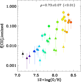
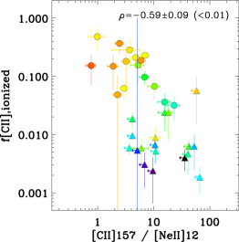
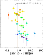
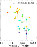
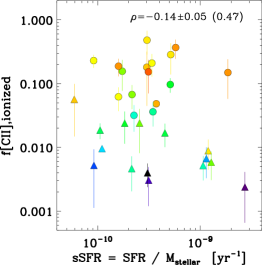
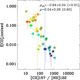
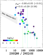
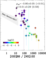
In Figure 10, we present correlations of the fractions of [C ii] emission from the ionized gas, , obtained from our models with free, with metallicity, specific star-formation rate (sSFR) and several combinations of observed line ratios to see if it is possible to predict the [C ii] fractions more easily (from observables rather than modeling). We quantified correlations using the IDL procedure r_correlate.pro which outputs the Spearman’s rank correlation coefficient and the two-sided significance of its deviation from zero. Here, we vary quantities within their uncertainties a 1,000 times to obtain a distribution of correlation coefficients. The plots report the median value the standard deviation of the distribution, as well as the median value of the significance distribution in parenthesis. As seen in Fig. 10 (and already noted in Fig. 9), is correlated with metallicity. is not correlated with sSFR. Regarding observed line ratios, we find the strongest trends with [C ii]/[Ne ii], [Ne iii]/[Ne ii], and [S iv]/[S iii]18. We also find strong trends of with [C ii]/[N ii]122 and [O iii]/[N ii]122 when taking into account predictions of [N ii]122 in addition to observations. The trends with [Ne iii]/[Ne ii], [S iv]/[S iii]18, and [O iii]/[N ii]122 can be understood as those ratios trace the average radiation field strength and, indirectly, metallicity. Regarding the [O iii]/[N ii]122 ratio, we overlay in Fig. 10 the fit of Díaz-Santos et al. (2017) for local luminous galaxies. We find a similar but offset trend, the dwarfs probing higher ratios of [O iii]/[N ii]122. We do not find any trend of with the [S iii] line ratio, which is a density tracer, though sensitive to higher densities than the critical density of [C ii] with electrons. From our model results, we find a weak anticorrelation between electron densities and , but with a lot of scatter. Hence, as in Díaz-Santos et al. (2017), correlates more strongly with the radiation field intensity than with the electron density (conveyed in the color coding of the last two panels of Fig. 10, and see also Fig. 16 in the appendix).
Accurso et al. (2017) and Olsen et al. (2017) investigate the [C ii] emission based on simulations of galaxies. In general, they find larger fractions of [C ii] in the ionized gas than we find here. Equation 16 of Accurso et al. (2017) provides a prescription of the fraction of [C ii] associated with PDRs that depends (only) on a galaxy’s sSFR. This prescription predicts that 55-75% of the [C ii] emission in our galaxies should arise from the PDR, which is somewhat coherent with our results. However, their Equation 12, which also depends on the dust mass fraction, , and electron density that we set to 30 cm-3, brings those fractions below 50%. Olsen et al. (2017) also find that the [C ii] emission from PDRs is below 50% in simulations of high-redshift star-forming galaxies. Those fractions of [C ii] emission arising from the PDR are low compared to our results and to Croxall et al. (2017). This discrepancy might be related to the fact that a two-phase model is a simplistic view of a galaxy, or alternatively that prescriptions or simulations are not representative of our population of galaxies, each galaxy being dominated by a few localized star-forming events.
Finally, our results may have implications for the use of [C ii] as a SFR indicator. Most of the [C ii] emission arises in PDRs at low metallicities, which indicates that the [C ii]157 line could still be a good tracer of the SFR in the low- galaxies at high redshift (see also Stacey et al., 2010; Vallini et al., 2015; Lagache et al., 2018). De Looze et al. (2014) found an offset in the [C ii]-SFR relation between nearby dwarf galaxies, and normal star-forming spirals and IR-luminous galaxies. This offset might be linked to contamination of the ionized gas to the observed [C ii] emission, resulting in higher [C ii] level of emission for a given level of SFR in metal-rich galaxies. Given our results and those of Croxall et al. (2017) on higher- galaxies, the contamination of the ionized gas to the observed [C ii] emission remains however moderate. Another important factor to consider in the [C ii]-SFR relation is the [C ii] line deficit (with respect to ) which varies by orders of magnitude in galaxies. This line deficit is closely related to the surface density of star formation and therefore probably to local variations of the dense gas conditions (Smith et al., 2017).
6.2 Correlation of modeled physical conditions, metallicity, and SFR
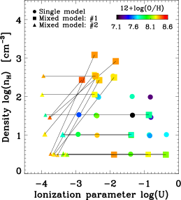
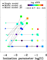
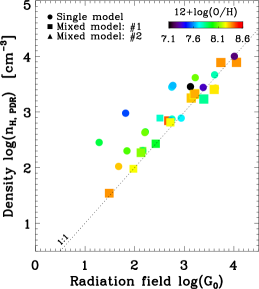
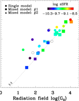
We aim to see if we can link the physical conditions, namely the density and radiation field in the H ii regions and PDRs, to more global parameters such as and sSFR. Figure 11 shows the model parameters of each galaxy with color codes corresponding to and sSFR.
Regarding the model parameters of the grid (top panels in Fig. 11), we find that there are no obvious systematics in the distribution of mixed models. For several galaxies, the mixed models highlight a need to have components with different rather than different . There is a tendency for the low- models to also have smaller scaling factors. Galaxies with higher tend to have lower ionization parameters than galaxies with lower (see also Fig. 16 in the appendix). Low-to-moderate ionization parameters () are indeed found in more metal-rich nearby galaxies (e.g., Herrera-Camus et al., 2018b). It is in the dwarf galaxies with lower that we find the highest values (). Finally, galaxies with higher sSFR tend to have higher than galaxies with lower sSFR.
Regarding the PDR parameters (bottom panels in Fig. 11), we find a clear correlation between and . We also find a tendency for lower- galaxies to have higher and values, but that tendency is clearer for high sSFR galaxies. Malhotra et al. (2001) conducted a study on nearby normal star-forming galaxies. They also found a relation between and , with , and explain that such scaling is expected from H ii regions (Strömgren spheres) surrounded by PDRs. The ratio of the two, , drives the heating of the PDR (e.g., Tielens & Hollenbach, 1985) and, interestingly, it is roughly constant in the galaxies of our sample. We find a median value of and a standard deviation of 0.4 dex. This is in the same range of values found by Díaz-Santos et al. (2017) for IR-luminous galaxies. High sSFR galaxies also have slightly higher values than the median, indicating more compact/intense star-forming regions, consistent with the increase of at high IR surface densities (though for more moderate values of and in our sample) reported by Díaz-Santos et al. (2017). Analytically, given our adopted density law, is proportional to . Since we find that lower- galaxies tend to have higher- values, this naturally leads to a roughly constant ratio. However, a constant ratio is not purely a consequence of model assumptions because the PDR parameters have to fit the (PDR) observations. A different density law would lead to a similar relation.
6.3 Phase filling factors
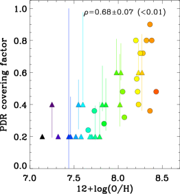
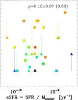
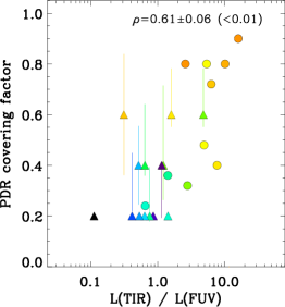
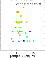
One main result from analyzing Spitzer and Herschel observations of both resolved regions and entire galaxies is that the ionized phase is extended and fills a large volume of the ISM of star-forming dwarf galaxies (Cormier et al., 2012; Chevance et al., 2016; Polles et al., 2019). With the modeling that we have performed for each individual galaxy of the Herschel DGS, we can quantify further the relative filling factor of the ionized and PDR phases. First, we investigate the relative volume filling factor of the two ionized gas components in the case of mixed models. We could expect a diffuse, low-excitation ionized medium to fill a larger volume than denser H ii regions. This is indeed the case for galaxies where the two components have very different densities (for example, Haro 11 and NGC 5253 for which the diffuse phase fills a volume that is about ten and one hundred times larger than the dense phase, respectively). However, as discussed in the previous section (Fig 11, top panels), we do not find a systematic contrast in density for the mixed models, even in galaxies where [N ii]122 is detected. In particular, the [O iii] emission, often found extended in studies that have sufficient spatial resolution (Chevance et al., 2016; Polles et al., 2019), is well reproduced by the high- (not necessarily low density) models.
Second, we investigate the covering factor of the PDR phase relative to that of the ionized phase. Figure 12 shows the PDR covering factors of the models as a function of metallicity, sSFR, and selected line ratios. The covering factor is simply the fraction of solid angle covered by PDR gas as seen from the center of the ionized region. For the mixed models, it is the product of the covering factor of the dense model multiplied by the scaling factor (the covering factor of the low-density model being set to zero by default). Correlating the PDR covering factor with several line ratios, such as [O iii]88/[C ii]157, [O iii]88/, or the optical line ratio of [O iii] 5007 Å -to- [O ii] 3727 Å, does not yield strong trends. Although the dwarf galaxies are offset in the observed parameter space of those ratios compared to metal-rich galaxies (Cormier et al., 2015), we do not find a robust line ratio predictor of the PDR covering factor (i.e., ISM porosity). It seems that the emission of the lines under study is too dependent on the other physical conditions and only the combination of many constraints provided by various lines can predict such parameter. However, we find that there is a correlation between the PDR covering factor and both the broadband luminosity ratio of / and , with large scatter. The trend indicates that the porosity of the ISM (relative covering factors of ionized and PDR gas) increases at low .
A decrease of the PDR covering factor may facilitate the escape of ionizing photons from the star-forming regions. Although our models by design cannot be used to quantify this escape, it is still a parameter worth discussing. In the Magellanic Clouds (with and , where ; Asplund et al. 2009), the fraction of ionizing photons escaping H ii regions is of the order of % (Pellegrini et al., 2012). Moreover, Gazagnes et al. (2018) show for galaxies with known Lyman continuum leakage that the escape of ionizing photons is related to the covering factor of the H i gas (rather than low H i column densities). Recent modeling of the Local Group dwarf galaxy IC 10 also shows that on scales of individual star-forming regions, clouds tend to be matter-bounded, allowing for the possibility of photons escaping the regions, while on larger spatial scales, clouds tend to be more radiation-bounded (Polles et al., 2019). At large enough scales the escape fraction is expected to be near zero. However, given that our models are radiation-bounded (i.e., we stopped them further than the ionization front) and that several nearby dwarf galaxies have extended H i halos that we have not modeled, the PDR covering factors derived here cannot be translated into galaxy escape fractions. Such escape fractions have been measured to be up to a few percent in nearby dwarf galaxies (e.g., Leitet et al. 2011, 2013; see also Zastrow et al. 2013), but could be larger in dwarfs at higher redshift (Razoumov & Sommer-Larsen, 2010; Yajima et al., 2011). Leitet et al. (2013) find that the escape fraction is somewhat larger in galaxies with lower metallicity, lower stellar mass and higher sSFR for the energetics of the star-forming regions to affect the whole galaxy (Clarke & Oey, 2002). Here, we find correlations between the PDR covering factor and metallicity (as well as with stellar mass and SFR) but not with sSFR. A lower PDR covering factor in nearby low- galaxies might indicate that the escape fraction is likely to be higher for low- galaxies in the high-redshift Universe.
7 Conclusions
We have modeled the MIR and FIR emission of the ISM of galaxies from the Herschel Dwarf Galaxy Survey with the spectral synthesis code Cloudy. The goal of this study is to characterize the gas physical conditions in the H ii region and PDR of those galaxies (namely density, ionization parameter, covering factor of the PDR), and to understand how or if they correlate with a galaxy’s metallicity or star-formation activity. We focus our discussion on the phase origin of [C ii] emission and on the ISM porosity. Our results are summarized as follows.
-
•
Several galaxies are well reproduced by single models, but for other galaxies we need mixed models, especially models with a different ionization parameter (rather than a different gas density) to reproduce satisfyingly the observed MIR-FIR emission. We find values of ionization parameters in the range to , and electron densities in the range cm-3, corresponding to PDR densities roughly ten times larger (given the adopted density profile). The highest values are higher than in metal-rich galaxies and are found in the lower- galaxies of our sample. Radiation fields and densities in the PDR are also found higher for the lowest- galaxies. Densities are higher in galaxies with higher specific star-formation rates.
-
•
We evaluated the effect of the choice of spectral lines to fit and of individual input parameters of the models on the results. The ionization parameter is mainly sensitive to the choice of input radiation field library, while choices on the density profile and dust-to-gas ratio can affect the density in the PDR. We find the need for a low-luminosity soft X-ray component and/or increased cosmic ray rate to reproduce the observed [O i]145/[O i]63 line ratios.
-
•
The contribution of the ionized phase to the [C ii] emission is low, typically 30%, making [C ii] a good tracer of PDRs and of the SFR at low metallicities (and potentially at high redshift). As found in Croxall et al. (2017), there is a trend of increasing [C ii] fractions from the ionized gas with metallicity, though with scatter. This fraction seems more driven by the ionization parameter (and indirectly metallicity) than by density.
-
•
We find that the covering factor of the neutral gas relative to that of the ionized gas decreases with decreasing metallicity and TIR-to-FUV luminosity ratio. This provides evidence for a change in the ISM porosity, which we conjecture may facilitate the propagation and escape of ionizing photon in some systems. If such ISM porosity is present in low-metallicity galaxies at high redshift, this might have implications for the fraction of escaping photons and cosmic reionization.
The DGS galaxies span more than an order of magnitude in metallicity and sSFR with a bias toward high sSFR values. Metallicity (rather than sSFR) seems to be the main parameter driving variations in the ISM properties of the DGS galaxies. However, extending the modeling approach of this paper to galaxies that cover a larger parameter space in terms of metallicity, SFR, stellar mass, amongst others, will be important to map the evolution of ISM properties through cosmic times.
Our suite of models makes predictions for many more lines than observed and discussed in this paper. These predictions will be used to guide follow-up observations that will allow us to exploit unique PDR coolants, such as [C i] (available with ALMA), MIR H2 and PAH features (available with the JWST), and to test the importance of specific heating mechanisms, such as shocks. Spatially resolving the main ISM phases would also be extremely useful for a more direct confirmation of the phase origin of the emission lines, respective filling factors, ISM porosity and potentially, the escape of ionizing photons.
Acknowledgements.
The authors thank P. De Vis for providing the Magphys SED of Haro 11 and M. Krumholz for useful discussion. We also thank the referee for the valuable comments which helped to improve the manuscript. DC is supported by the European Union’s Horizon 2020 research and innovation program under the Marie Skłodowska-Curie grant agreement No 702622. NPA acknowledges funding from NASA and SOFIA through grant program SOF 05-0084. SH is supported by the DFG program HO 5475/2-1. IDL gratefully acknowledges the support of the Research Foundation – Flanders (FWO). We also acknowledge support from the DAAD/PROCOPE projects 57210883/35265PE and from the Programme National “Physique et Chimie du Milieu Interstellaire” (PCMI) of CNRS/INSU with INC/INP co-funded by CEA and CNES.References
- Abdullah et al. (2017) Abdullah, A., Brandl, B. R., Groves, B., et al. 2017, ApJ, 842, 4
- Abel et al. (2009) Abel, N. P., Dudley, C., Fischer, J., Satyapal, S., & van Hoof, P. A. M. 2009, ApJ, 701, 1147
- Abel et al. (2005) Abel, N. P., Ferland, G. J., Shaw, G., & van Hoof, P. A. M. 2005, ApJS, 161, 65
- Abel et al. (2007) Abel, N. P., Sarma, A. P., Troland, T. H., & Ferland, G. J. 2007, ApJ, 662, 1024
- Abel et al. (2008) Abel, N. P., van Hoof, P. A. M., Shaw, G., Ferland, G. J., & Elwert, T. 2008, ApJ, 686, 1125
- Accurso et al. (2017) Accurso, G., Saintonge, A., Bisbas, T. G., & Viti, S. 2017, MNRAS, 464, 3315
- Annibali et al. (2015) Annibali, F., Tosi, M., Pasquali, A., et al. 2015, AJ, 150, 143
- Asplund et al. (2009) Asplund, M., Grevesse, N., Sauval, A. J., & Scott, P. 2009, ARA&A, 47, 481
- Brauher et al. (2008) Brauher, J. R., Dale, D. A., & Helou, G. 2008, ApJS, 178, 280
- Chevance et al. (2016) Chevance, M., Madden, S. C., Lebouteiller, V., et al. 2016, A&A, 590, A36
- Cigan et al. (2016) Cigan, P., Young, L., Cormier, D., et al. 2016, AJ, 151, 14
- Clarke & Oey (2002) Clarke, C. & Oey, M. S. 2002, MNRAS, 337, 1299
- Cormier et al. (2012) Cormier, D., Lebouteiller, V., Madden, S. C., et al. 2012, A&A, 548, A20
- Cormier et al. (2015) Cormier, D., Madden, S. C., Lebouteiller, V., et al. 2015, A&A, 578, A53
- Cormier et al. (2014) Cormier, D., Madden, S. C., Lebouteiller, V., et al. 2014, A&A, 564, A121
- Croxall et al. (2017) Croxall, K. V., Smith, J. D., Pellegrini, E., et al. 2017, ApJ, 845, 96
- da Cunha et al. (2008) da Cunha, E., Charlot, S., & Elbaz, D. 2008, MNRAS, 388, 1595
- Dale et al. (2009) Dale, D. A., Smith, J. D. T., Schlawin, E. A., et al. 2009, ApJ, 693, 1821
- Dalgarno (2006) Dalgarno, A. 2006, Proceedings of the National Academy of Science, 103, 12269
- De Looze et al. (2011) De Looze, I., Baes, M., Bendo, G. J., Cortese, L., & Fritz, J. 2011, MNRAS, 416, 2712
- De Looze et al. (2014) De Looze, I., Cormier, D., Lebouteiller, V., et al. 2014, A&A, 568, A62
- De Vis et al. (2017) De Vis, P., Gomez, H. L., Schofield, S. P., et al. 2017, MNRAS, 471, 1743
- Díaz-Santos et al. (2017) Díaz-Santos, T., Armus, L., Charmandaris, V., et al. 2017, ApJ, 846, 32
- Díaz-Santos et al. (2013) Díaz-Santos, T., Armus, L., Charmandaris, V., et al. 2013, ApJ, 774, 68
- Dimaratos et al. (2015) Dimaratos, A., Cormier, D., Bigiel, F., & Madden, S. C. 2015, A&A, 580, A135
- Ferland et al. (2017) Ferland, G. J., Chatzikos, M., Guzmán, F., et al. 2017, Rev. Mexicana Astron. Astrofis., 53, 385
- Fernández-Ontiveros et al. (2016) Fernández-Ontiveros, J. A., Spinoglio, L., Pereira-Santaella, M., et al. 2016, ApJS, 226, 19
- Garnett et al. (1995) Garnett, D. R., Skillman, E. D., Dufour, R. J., et al. 1995, ApJ, 443, 64
- Gazagnes et al. (2018) Gazagnes, S., Chisholm, J., Schaerer, D., et al. 2018, A&A, 616, A29
- Gil de Paz et al. (2003) Gil de Paz, A., Madore, B. F., & Pevunova, O. 2003, ApJS, 147, 29
- Guseva et al. (2012) Guseva, N. G., Izotov, Y. I., Fricke, K. J., & Henkel, C. 2012, A&A, 541, A115
- Habing (1968) Habing, H. J. 1968, Bull. Astron. Inst. Netherlands, 19, 421
- Hennebelle & Chabrier (2008) Hennebelle, P. & Chabrier, G. 2008, ApJ, 684, 395
- Herrera-Camus et al. (2016) Herrera-Camus, R., Bolatto, A., Smith, J. D., et al. 2016, ApJ, 826, 175
- Herrera-Camus et al. (2015) Herrera-Camus, R., Bolatto, A. D., Wolfire, M. G., et al. 2015, ApJ, 800, 1
- Herrera-Camus et al. (2018a) Herrera-Camus, R., Sturm, E., Graciá-Carpio, J., et al. 2018a, ApJ, 861, 94
- Herrera-Camus et al. (2018b) Herrera-Camus, R., Sturm, E., Graciá-Carpio, J., et al. 2018b, ApJ, 861, 95
- Hollenbach & Tielens (1999) Hollenbach, D. J. & Tielens, A. G. G. M. 1999, Reviews of Modern Physics, 71, 173
- Hopkins et al. (2012) Hopkins, P. F., Quataert, E., & Murray, N. 2012, MNRAS, 421, 3488
- Hosokawa & Inutsuka (2005) Hosokawa, T. & Inutsuka, S.-i. 2005, ApJ, 623, 917
- Houck et al. (2004) Houck, J. R., Roellig, T. L., Van Cleve, J., et al. 2004, in Society of Photo-Optical Instrumentation Engineers (SPIE) Conference Series, Vol. 5487, Society of Photo-Optical Instrumentation Engineers (SPIE) Conference Series, ed. J. C. Mather, 62–76
- Houck et al. (1984) Houck, J. R., Shure, M. A., Gull, G. E., & Herter, T. 1984, ApJ, 287, L11
- Hughes et al. (2015) Hughes, T. M., Foyle, K., Schirm, M. R. P., et al. 2015, A&A, 575, A17
- Hummer & Storey (1987) Hummer, D. G. & Storey, P. J. 1987, MNRAS, 224, 801
- Hunt et al. (2010) Hunt, L. K., Thuan, T. X., Izotov, Y. I., & Sauvage, M. 2010, ApJ, 712, 164
- Hunter et al. (2001) Hunter, D. A., Kaufman, M., Hollenbach, D. J., et al. 2001, ApJ, 553, 121
- Indebetouw et al. (2013) Indebetouw, R., Brogan, C., Chen, C.-H. R., et al. 2013, ApJ, 774, 73
- Indriolo et al. (2007) Indriolo, N., Geballe, T. R., Oka, T., & McCall, B. J. 2007, ApJ, 671, 1736
- Izotov et al. (2006) Izotov, Y. I., Papaderos, P., Guseva, N. G., Fricke, K. J., & Thuan, T. X. 2006, A&A, 454, 137
- Izotov & Thuan (1999) Izotov, Y. I. & Thuan, T. X. 1999, ApJ, 511, 639
- Izotov & Thuan (2004) Izotov, Y. I. & Thuan, T. X. 2004, ApJ, 616, 768
- Jameson et al. (2018) Jameson, K. E., Bolatto, A. D., Wolfire, M., et al. 2018, ApJ, 853, 111
- Kaufman et al. (2006) Kaufman, M. J., Wolfire, M. G., & Hollenbach, D. J. 2006, ApJ, 644, 283
- Kaufman et al. (1999) Kaufman, M. J., Wolfire, M. G., Hollenbach, D. J., & Luhman, M. L. 1999, ApJ, 527, 795
- Keenan & Conlon (1993) Keenan, F. P. & Conlon, E. S. 1993, ApJ, 410, 426
- Kobulnicky & Skillman (1996) Kobulnicky, H. A. & Skillman, E. D. 1996, ApJ, 471, 211
- Kobulnicky et al. (1997) Kobulnicky, H. A., Skillman, E. D., Roy, J.-R., Walsh, J. R., & Rosa, M. R. 1997, ApJ, 477, 679
- Kroupa (2001) Kroupa, P. 2001, MNRAS, 322, 231
- Lagache et al. (2018) Lagache, G., Cousin, M., & Chatzikos, M. 2018, A&A, 609, A130
- Lapham et al. (2017) Lapham, R. C., Young, L. M., & Crocker, A. 2017, ApJ, 840, 51
- Lebouteiller et al. (2008) Lebouteiller, V., Bernard-Salas, J., Brandl, B., et al. 2008, ApJ, 680, 398
- Lebouteiller et al. (2017) Lebouteiller, V., Péquignot, D., Cormier, D., et al. 2017, A&A, 602, A45
- Leitet et al. (2013) Leitet, E., Bergvall, N., Hayes, M., Linné, S., & Zackrisson, E. 2013, A&A, 553, A106
- Leitet et al. (2011) Leitet, E., Bergvall, N., Piskunov, N., & Andersson, B.-G. 2011, A&A, 532, A107
- Leitherer et al. (2010) Leitherer, C., Ortiz Otálvaro, P. A., Bresolin, F., et al. 2010, ApJS, 189, 309
- Liseau et al. (2006) Liseau, R., Justtanont, K., & Tielens, A. G. G. M. 2006, A&A, 446, 561
- Madden et al. (2006) Madden, S. C., Galliano, F., Jones, A. P., & Sauvage, M. 2006, A&A, 446, 877
- Madden et al. (2013) Madden, S. C., Rémy-Ruyer, A., Galametz, M., et al. 2013, PASP, 125, 600
- Malhotra et al. (2001) Malhotra, S., Kaufman, M. J., Hollenbach, D., et al. 2001, ApJ, 561, 766
- Meijerink & Spaans (2005) Meijerink, R. & Spaans, M. 2005, A&A, 436, 397
- Mollá et al. (2009) Mollá, M., García-Vargas, M. L., & Bressan, A. 2009, MNRAS, 398, 451
- Morisset & Georgiev (2009) Morisset, C. & Georgiev, L. 2009, A&A, 507, 1517
- Naab & Ostriker (2017) Naab, T. & Ostriker, J. P. 2017, ARA&A, 55, 59
- Neufeld & Wolfire (2017) Neufeld, D. A. & Wolfire, M. G. 2017, ApJ, 845, 163
- Oberst et al. (2006) Oberst, T. E., Parshley, S. C., Stacey, G. J., et al. 2006, ApJ, 652, L125
- O’Halloran et al. (2008) O’Halloran, B., Madden, S. C., & Abel, N. P. 2008, ApJ, 681, 1205
- Olsen et al. (2017) Olsen, K., Greve, T. R., Narayanan, D., et al. 2017, ApJ, 846, 105
- Osterbrock & Ferland (2006) Osterbrock, D. E. & Ferland, G. J. 2006, Astrophysics of gaseous nebulae and active galactic nuclei
- Padovani & Galli (2011) Padovani, M. & Galli, D. 2011, A&A, 530, A109
- Parkin et al. (2014) Parkin, T. J., Wilson, C. D., Schirm, M. R. P., et al. 2014, ApJ, 787, 16
- Pellegrini et al. (2012) Pellegrini, E. W., Oey, M. S., Winkler, P. F., et al. 2012, ApJ, 755, 40
- Pilbratt et al. (2010) Pilbratt, G. L., Riedinger, J. R., Passvogel, T., et al. 2010, A&A, 518, L1+
- Pilyugin & Thuan (2005) Pilyugin, L. S. & Thuan, T. X. 2005, ApJ, 631, 231
- Pineda et al. (2013) Pineda, J. L., Langer, W. D., Velusamy, T., & Goldsmith, P. F. 2013, A&A, 554, A103
- Poglitsch et al. (2010) Poglitsch, A., Waelkens, C., Geis, N., et al. 2010, A&A, 518, L2+
- Polles et al. (2019) Polles, F. L., Madden, S. C., Lebouteiller, V., et al. 2019, A&A, 622, A119
- Press et al. (1992) Press, W. H., Teukolsky, S. A., Vetterling, W. T., & Flannery, B. P. 1992, Numerical recipes in FORTRAN. The art of scientific computing
- Razoumov & Sommer-Larsen (2010) Razoumov, A. O. & Sommer-Larsen, J. 2010, ApJ, 710, 1239
- Rémy-Ruyer et al. (2014) Rémy-Ruyer, A., Madden, S. C., Galliano, F., et al. 2014, A&A, 563, A31
- Rémy-Ruyer et al. (2015) Rémy-Ruyer, A., Madden, S. C., Galliano, F., et al. 2015, A&A, 582, A121
- Rosenberg et al. (2015) Rosenberg, M. J. F., van der Werf, P. P., Aalto, S., et al. 2015, ApJ, 801, 72
- Savage & Sembach (1996) Savage, B. D. & Sembach, K. R. 1996, ARA&A, 34, 279
- Smith et al. (2017) Smith, J. D. T., Croxall, K., Draine, B., et al. 2017, ApJ, 834, 5
- Spinoglio et al. (2017) Spinoglio, L., Alonso-Herrero, A., Armus, L., et al. 2017, PASA, 34, e057
- Stacey et al. (2010) Stacey, G. J., Hailey-Dunsheath, S., Ferkinhoff, C., et al. 2010, ApJ, 724, 957
- Stark (2016) Stark, D. P. 2016, ARA&A, 54, 761
- Thuan & Izotov (2005) Thuan, T. X. & Izotov, Y. I. 2005, ApJS, 161, 240
- Tielens (2005) Tielens, A. G. G. M. 2005, The Physics and Chemistry of the Interstellar Medium
- Tielens & Hollenbach (1985) Tielens, A. G. G. M. & Hollenbach, D. 1985, ApJ, 291, 722
- Turner et al. (2017) Turner, J. L., Consiglio, S. M., Beck, S. C., et al. 2017, ApJ, 846, 73
- Ucci et al. (2017) Ucci, G., Ferrara, A., Gallerani, S., & Pallottini, A. 2017, MNRAS, 465, 1144
- Vallini et al. (2017) Vallini, L., Ferrara, A., Pallottini, A., & Gallerani, S. 2017, MNRAS, 467, 1300
- Vallini et al. (2015) Vallini, L., Gallerani, S., Ferrara, A., Pallottini, A., & Yue, B. 2015, ApJ, 813, 36
- van der Tak et al. (2018) van der Tak, F. F. S., Madden, S. C., Roelfsema, P., et al. 2018, PASA, 35, e002
- Werner et al. (2004) Werner, M. W., Roellig, T. L., Low, F. J., et al. 2004, ApJS, 154, 1
- Westmoquette et al. (2013) Westmoquette, M. S., James, B., Monreal-Ibero, A., & Walsh, J. R. 2013, A&A, 550, A88
- Wolfire et al. (2010) Wolfire, M. G., Hollenbach, D., & McKee, C. F. 2010, ApJ, 716, 1191
- Wu et al. (2006) Wu, Y., Charmandaris, V., Hao, L., et al. 2006, ApJ, 639, 157
- Yajima et al. (2011) Yajima, H., Choi, J.-H., & Nagamine, K. 2011, MNRAS, 412, 411
- Zanella et al. (2018) Zanella, A., Daddi, E., Magdis, G., et al. 2018, MNRAS, 481, 1976
- Zastrow et al. (2013) Zastrow, J., Oey, M. S., Veilleux, S., & McDonald, M. 2013, ApJ, 779, 76
Appendix A Observed abundances for the DGS galaxies
In Table 6, we report the observed abundances from the literature for the galaxies of the Herschel Dwarf Galaxy Survey (Madden et al. 2013) studied here.
| Galaxy | ||||
|---|---|---|---|---|
| Haro 11 | … | |||
| Haro 2 | … | … | … | |
| Haro 3 | … | |||
| He 2-10 | … | … | … | |
| HS 0052+2536 | … | … | … | |
| HS 0822+3542 | … | … | ||
| HS 1222+3741 | … | … | … | |
| HS 1304+3529 | … | … | … | |
| HS 1330+3651 | … | … | … | |
| II Zw 40 | … | |||
| I Zw 18 | ||||
| Mrk 153 | … | … | … | |
| Mrk 209 | … | |||
| Mrk 930 | … | |||
| Mrk 1089 | … | |||
| Mrk 1450 | … | |||
| NGC 1140 | … | |||
| NGC 1569 | … | |||
| NGC 1705 | … | |||
| NGC 5253 | … | |||
| NGC 625 | … | … | … | |
| Pox 186 | … | … | … | |
| SBS 0335-052 | ||||
| SBS 1159+545 | … | |||
| SBS 1211+540 | … | |||
| SBS 1249+493 | … | |||
| SBS 1415+437 | ||||
| SBS 1533+574 | … | |||
| Tol 1214-277 | … | |||
| UM 448 | … | |||
| UM 461 | … | |||
| VII Zw 403 | … | |||
| NGC 4214-c | ||||
| NGC 4214-s | ||||
| Galaxy | ||||
| Haro 11 | … | |||
| Haro 3 | … | … | ||
| HS 0822+3542 | … | … | … | |
| II Zw 40 | … | … | … | |
| I Zw 18 | … | |||
| Mrk 209 | … | … | ||
| Mrk 930 | … | … | ||
| Mrk 1089 | … | … | ||
| Mrk 1450 | … | … | ||
| NGC 1140 | … | … | ||
| NGC 1569 | … | … | … | |
| NGC 1705 | … | … | ||
| NGC 5253 | … | … | ||
| SBS 0335-052 | … | |||
| SBS 1159+545 | … | … | … | |
| SBS 1211+540 | … | … | … | |
| SBS 1249+493 | … | … | … | |
| SBS 1415+437 | … | … | ||
| SBS 1533+574 | … | … | ||
| UM 448 | … | … | ||
| UM 461 | … | … | … | |
| VII Zw 403 | … | … | … | |
| NGC 4214-c | … | … | … | |
| NGC 4214-s | … | … | … |
Appendix B Atlas of the H ii region+PDR best-fitting model schematics
For each galaxy, we show a 2D schematic of the best-fitting single or mixed model, based on model results presented in Tables 3 and 4. Galaxies are sorted by metallicity (from highest to lowest). Color coding corresponds to density. The central stellar cluster is represented in green. The distance to the inner black shell varies with the inner radius, and the thickness of the inner black shell is proportional to the ionization parameter , while the thickness of the H ii and PDR regions are kept fixed. is a function of the input stellar spectrum, density, and inner radius. In the case of mixed models, the angle shown by dotted lines indicates the contribution from each component (i.e., parameter in Tables 3 and 4).
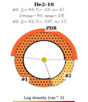
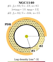
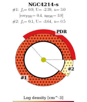
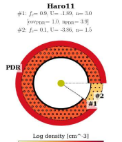
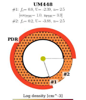
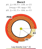
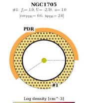
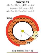
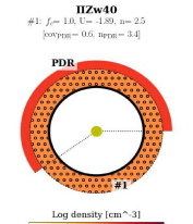
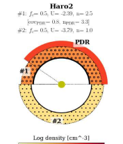
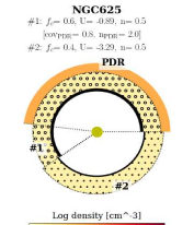
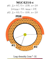
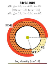
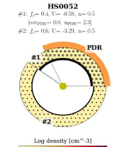
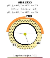
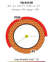

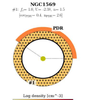
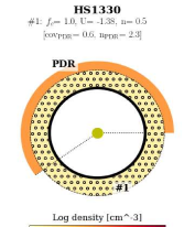
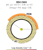
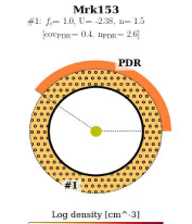
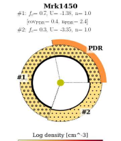
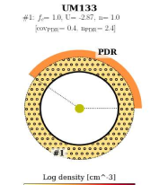
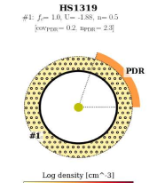
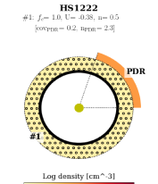
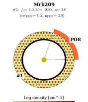
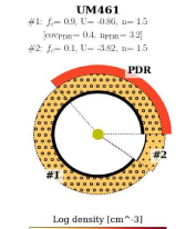
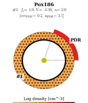
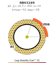
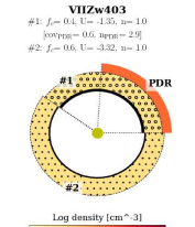
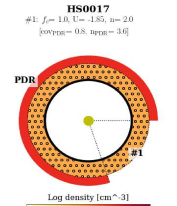
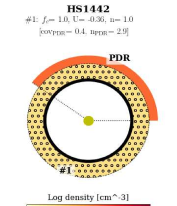
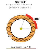


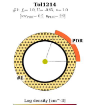
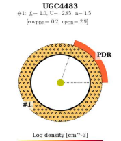
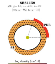
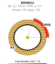
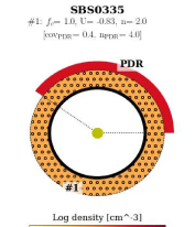
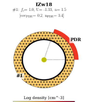

Appendix C Additional correlations for the galaxy sample
In Figure 16, we show correlations of the fraction of [C ii] emission from the ionized gas deduced from the models as a function of the model density and ionization parameter, as well as the correlation between the galaxy metallicity and the model ionization parameter.
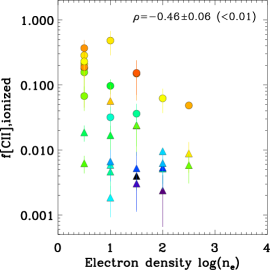
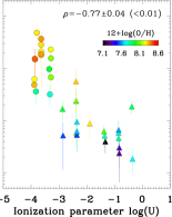
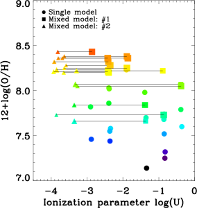
Appendix D Results of the H ii region+PDR models for individual galaxies
We show the results of the H ii region+PDR modeling of individual galaxies with three main types of plots: Comparison of the observed and predicted line intensities; Contribution of each gas component to the total line prediction in case of mixed models; Probability density functions (PDFs) of the fitted parameters. Only the results of the galaxy He 2-10 are shown in the main text of the paper (Fig. 4).
(a)
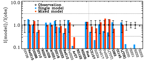 (b)
(b)
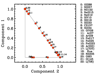
(c)
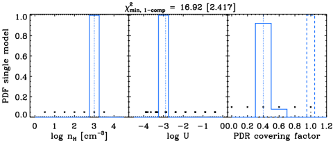
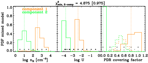
(a)
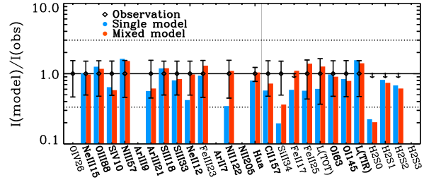 (b)
(b)
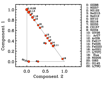
(c)
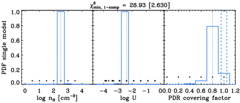
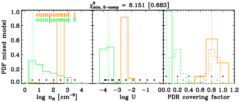
(a)
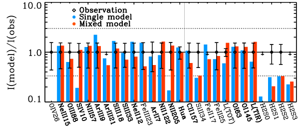 (b)
(b)

(c)
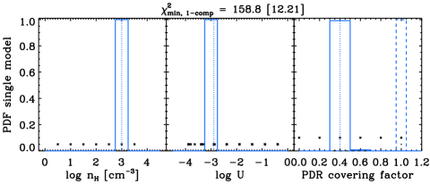
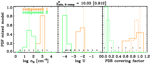
(a)
 (b)
(b)
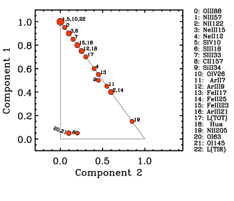
(c)
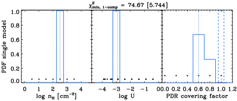
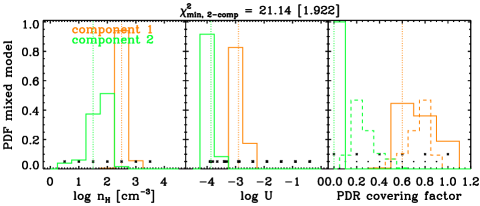
(a)
(b)
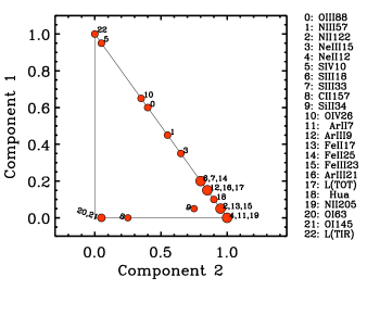
(c)
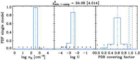
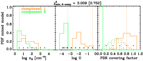
(a)
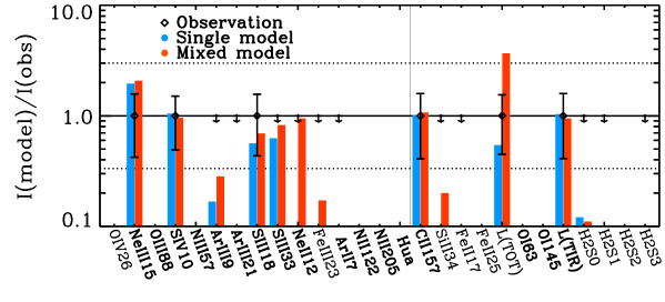 (b)
(b)
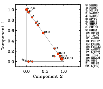
(c)
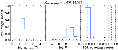
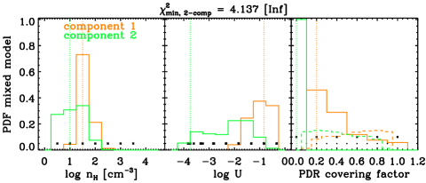
(a)
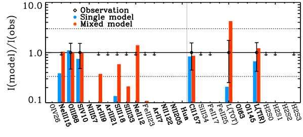 (b)
(b)
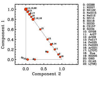
(c)
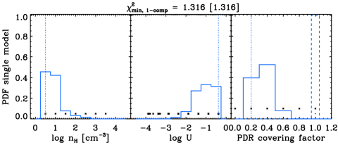
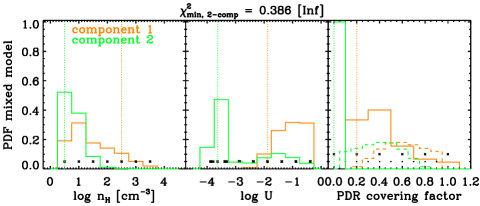
(a)
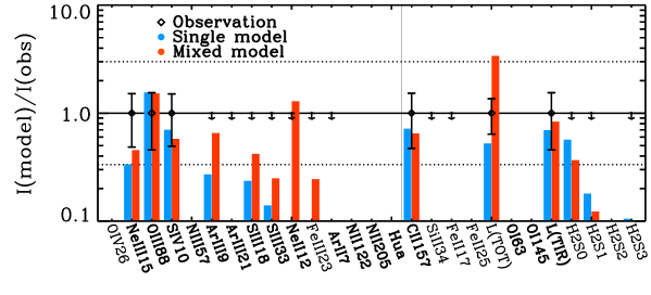 (b)
(b)
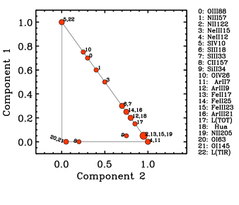
(c)
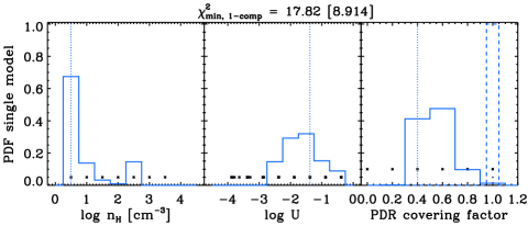
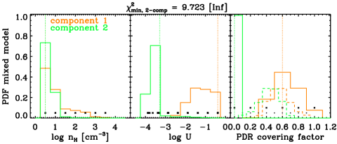
(a)
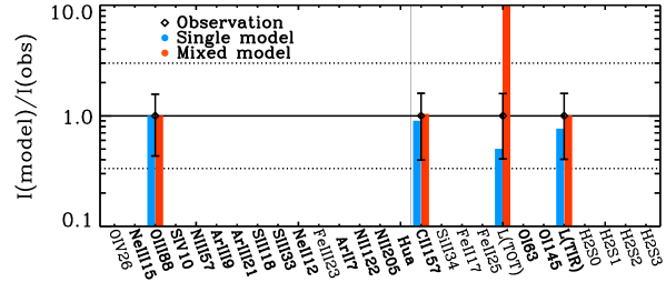 (b)
(b)
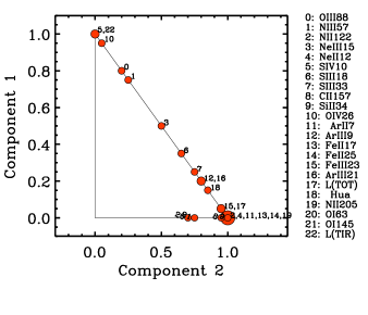
(c)
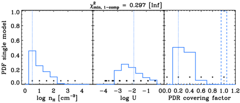
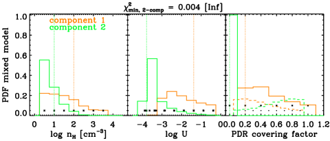
(a)
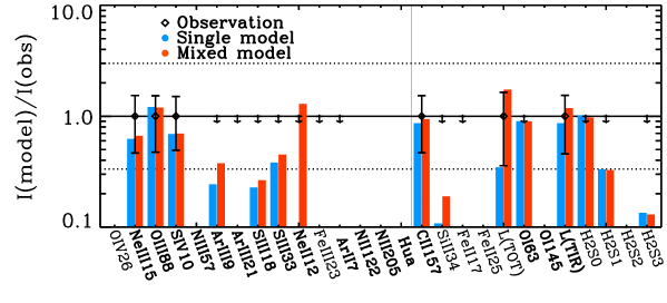 (b)
(b)
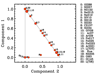
(c)
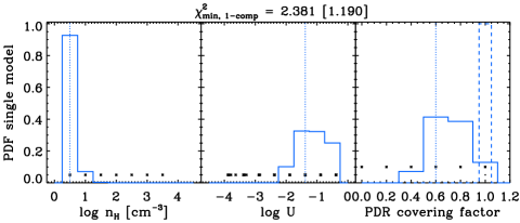
(a)
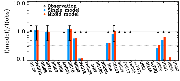 (b)
(b)
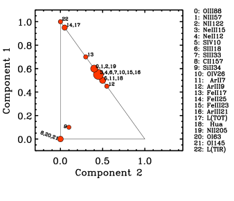
(c)
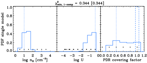
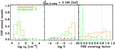
(a)
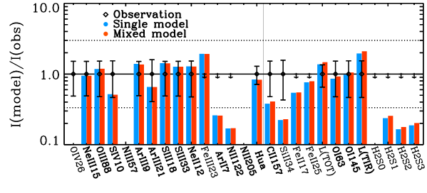 (b)
(b)
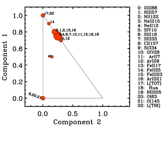
(c)
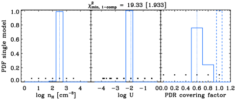
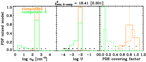
(a)
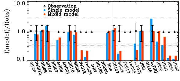 (b)
(b)
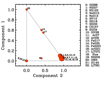
(c)
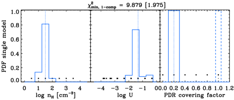
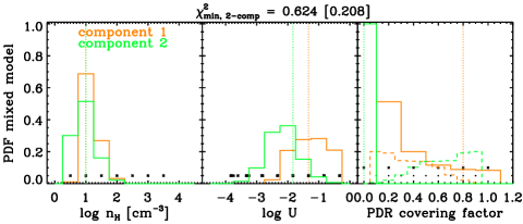
(a)
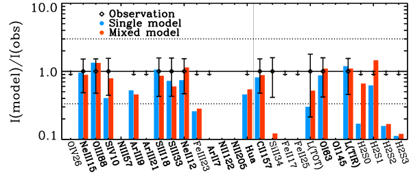 (b)
(b)
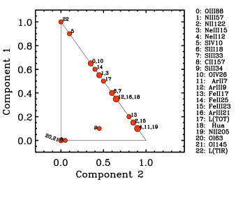
(c)
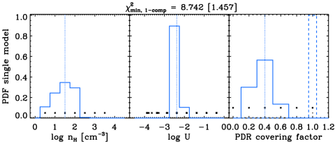
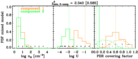
(a)
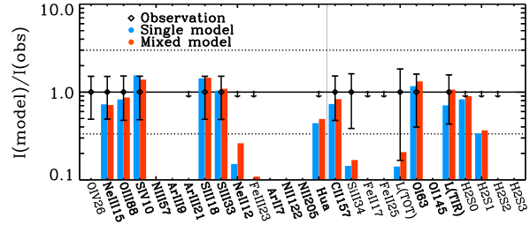 (b)
(b)
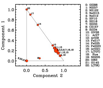
(c)
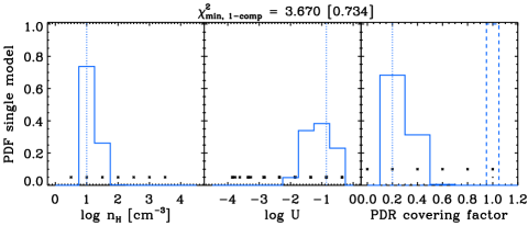
(a)
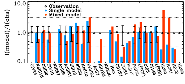 (b)
(b)
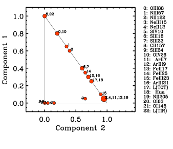
(c)
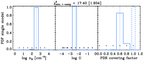
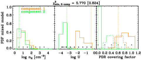
(a)
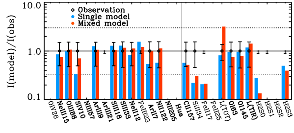 (b)
(b)
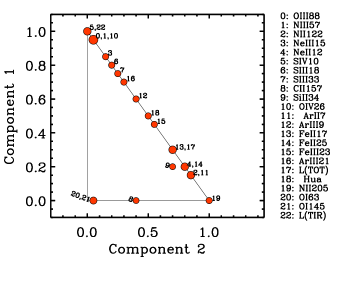
(c)
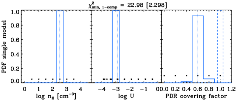
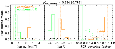
(a)
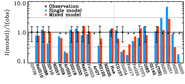 (b)
(b)
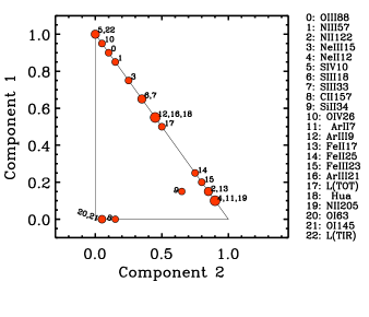
(c)
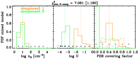
(a)
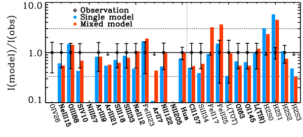 (b)
(b)
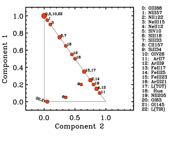
(c)
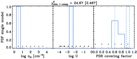
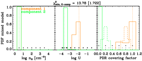
(a)
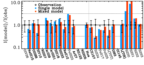 (b)
(b)
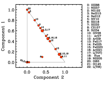
(c)
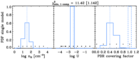

(a)
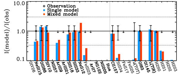 (b)
(b)
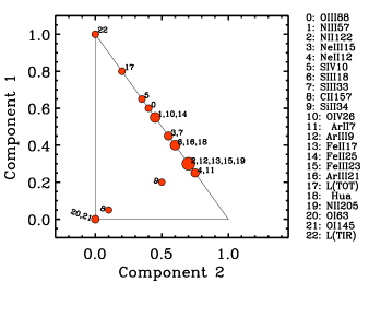
(c)
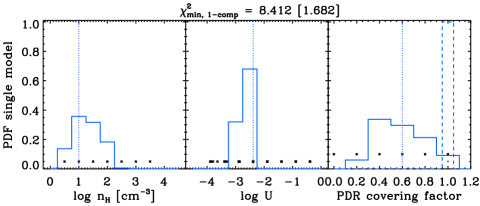
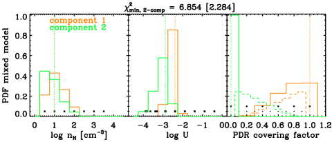
(a)
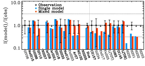 (b)
(b)
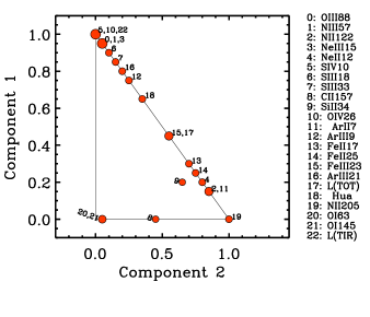
(c)
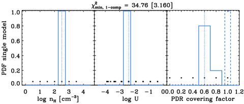
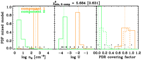
(a)
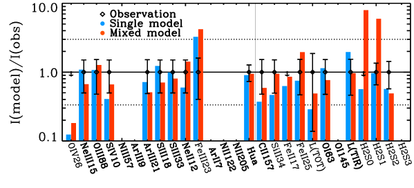 (b)
(b)
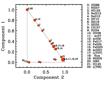
(c)
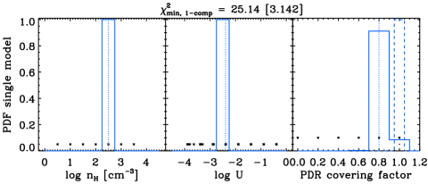
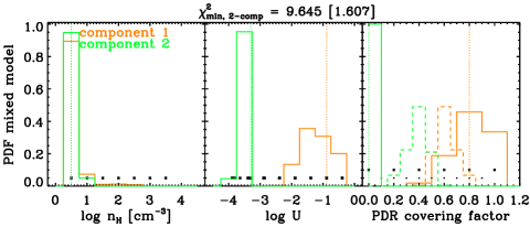
(a)
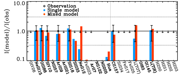 (b)
(b)
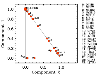
(c)
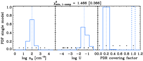
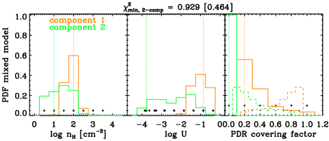
(a)
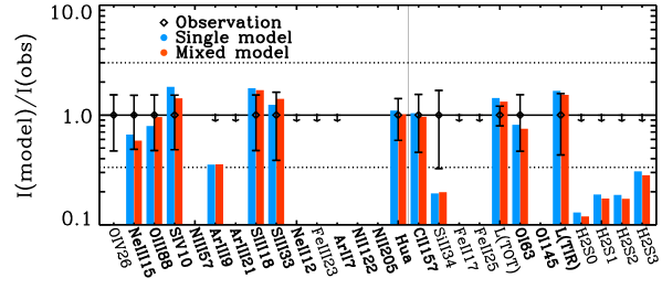 (b)
(b)
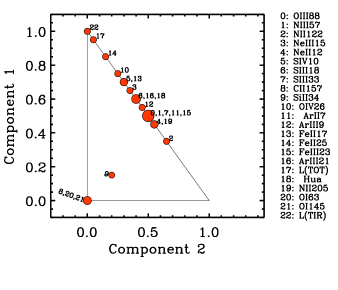
(c)
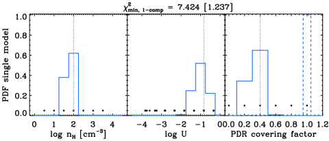
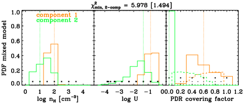
(a)
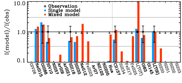 (b)
(b)
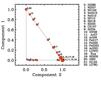
(c)
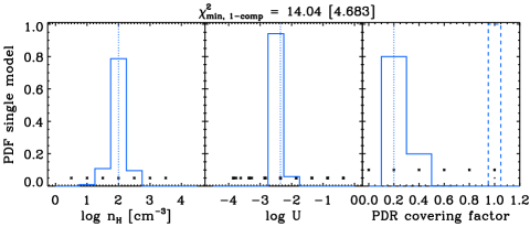
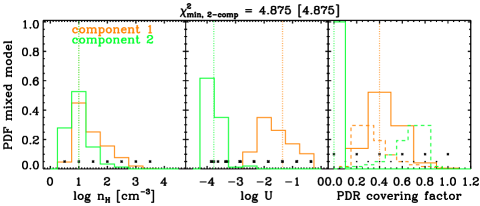
(a)
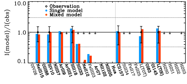 (b)
(b)
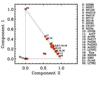
(c)
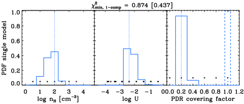
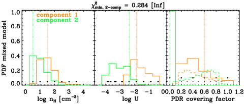
(a)
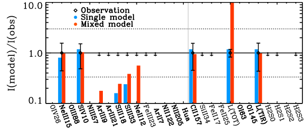 (b)
(b)
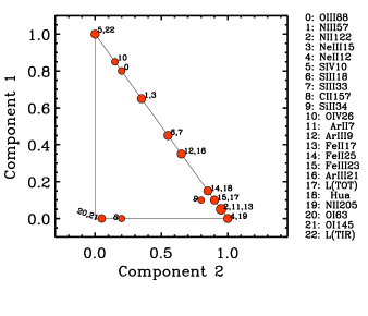
(c)
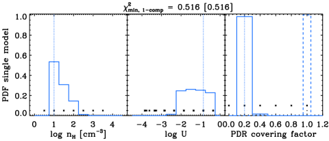
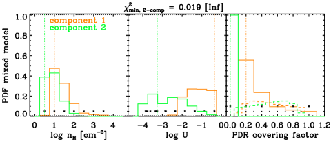
(a)
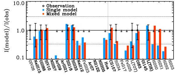 (b)
(b)
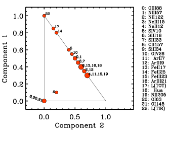
(c)
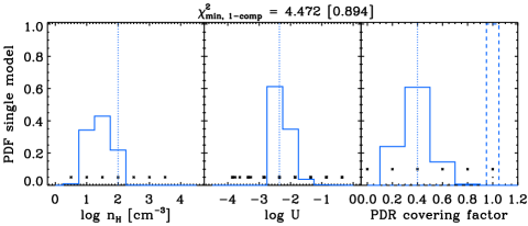
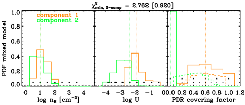
(a)
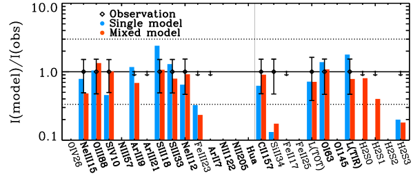 (b)
(b)
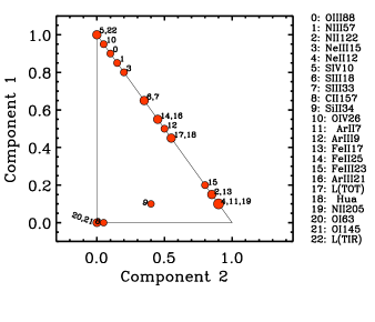
(c)
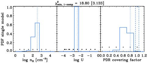
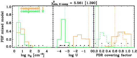
(a)
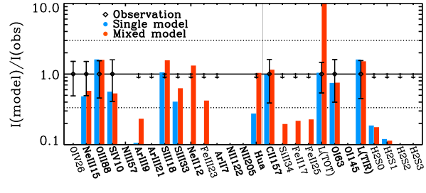 (b)
(b)
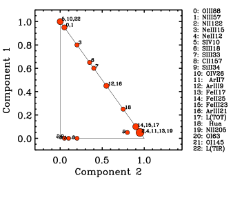
(c)
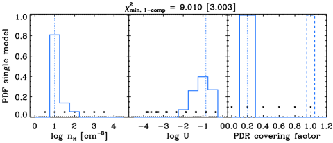
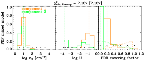
(a)
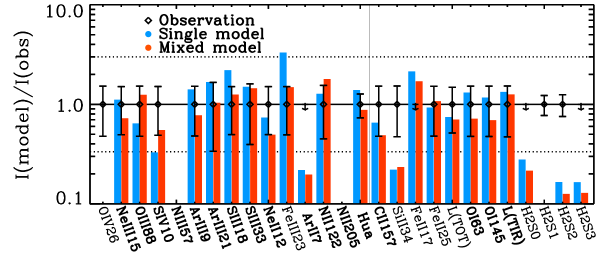 (b)
(b)
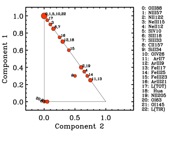
(c)
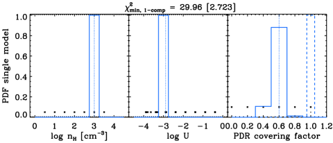
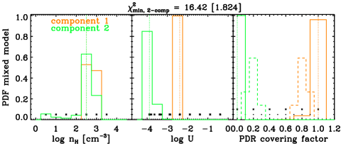
(a)
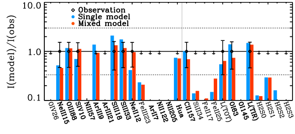 (b)
(b)
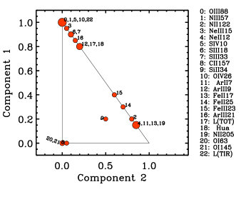
(c)
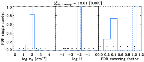
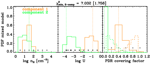
(a)
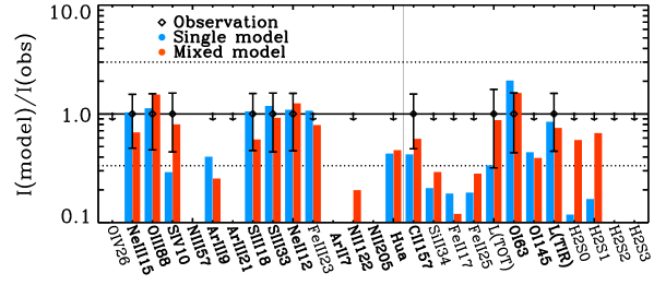 (b)
(b)
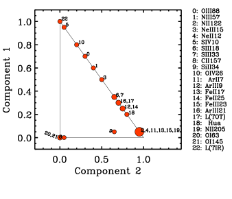
(c)
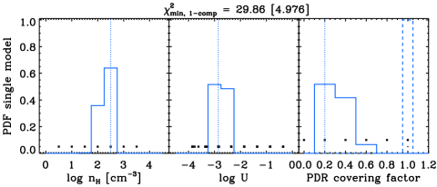
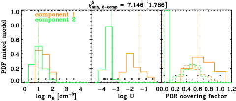
(a)
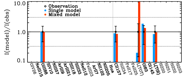 (b)
(b)
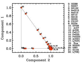
(c)
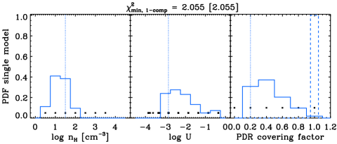
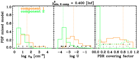
(a)
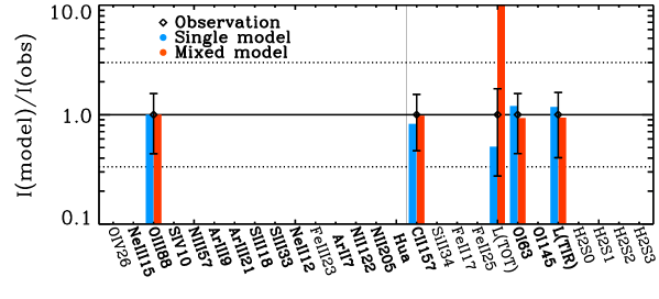 (b)
(b)
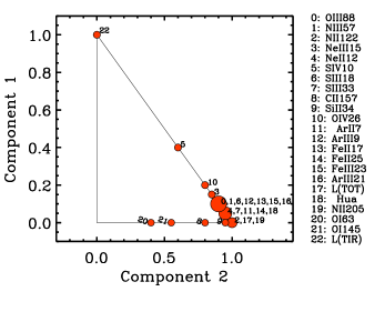
(c)
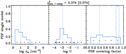
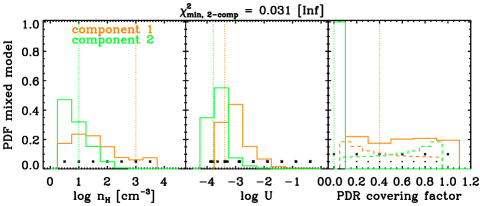
(a)
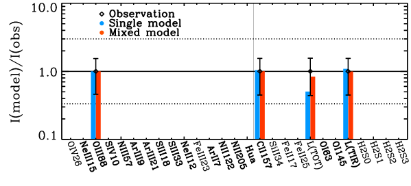 (b)
(b)
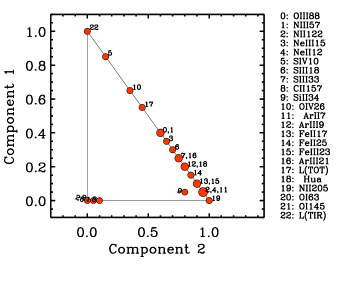
(c)
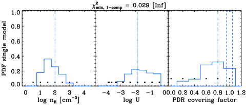
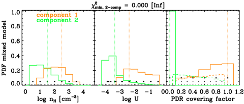
(a)
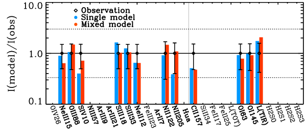 (b)
(b)
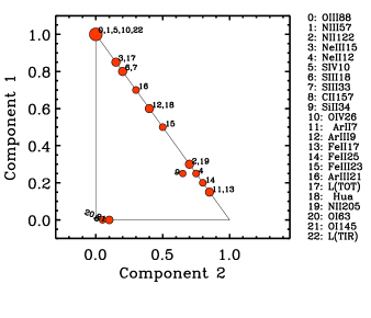
(c)
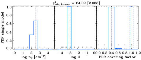
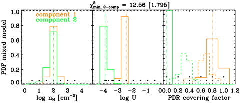
(a)
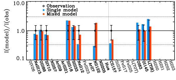 (b)
(b)
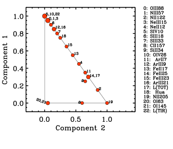
(c)
