RECOVERING THERMODYNAMICS FROM SPECTRAL PROFILES OBSERVED BY IRIS:
A MACHINE AND DEEP LEARNING APPROACH

Abstract

Inversion codes allow reconstructing a model atmosphere from observations. With the inclusion of optically thick lines that form in the solar chromosphere, such modelling is computationally very expensive because a non-LTE evaluation of the radiation field is required. In this study, we combine the results provided by these traditional methods with machine and deep learning techniques to obtain similar-quality results in an easy-to-use, much faster way. We have applied these new methods to Mg II h&k lines observed by IRIS. As a result, we are able to reconstruct the thermodynamic state (temperature, line-of-sight velocity, non-thermal velocities, electron density, etc.) in the chromosphere and upper photosphere of an area equivalent to an active region in a few CPU minutes, speeding up the process by a factor of $10^{5}-10^{6}$. The open-source code accompanying this paper will allow the community to use IRIS observations to open a new window to a host of solar phenomena.

1. Introduction

To answer some of the major open questions about the solar atmosphere, it is critical to understand the physical conditions in the chromosphere. The chromosphere has been observed for decades from ground- and space-based telescopes. Particularly the Interface Region Imaging Spectrograph explorer (De Pontieu et al., 2014, IRIS) has observed more than $\approx 19,000$ data sets at sub-arcsecond resolution in the Mg II h&k spectral range, in the near ultraviolet (NUV), since it was launched in 2013.

The formation of the Mg II h&k lines has been studied using numerical calculations that include the effect of partial redistribution of scattered photons and 3D radiative transfer effects (Leenaarts et al., 2013a, b; del Pino Alemán et al., 2016; Sukhorukov & Leenaarts, 2017). Some spectral features such as the intensity and wavelength of the emission peaks and central reversal of those lines can potentially serve as proxies of the temperature, line-of-sight velocity ($v_{los}$), and their gradients in various regions of the chromosphere (Leenaarts et al., 2013b; Pereira et al., 2015). However, so far these proxies have only been studied for quiet-Sun like conditions, and do not provide detailed height-dependent diagnostics.

One of the most successful methods to recover physical information from spectropolarimetric observations is through non-linear fitting techniques, where the parameters of a model atmosphere are iteratively adjusted in order to match the emerging model intensities with the observed spectra. This procedure is commonly called an ”inversion” even though it is not based on a formal inversion to the radiative transfer equation.

de la Cruz Rodríguez et al. (2016) and de la Cruz Rodríguez et al. (2018) have developed the STockholm Inversion Code (STiC) which assumes non-local thermodynamical equilibrium, plane-parallel geometry and includes partial frequency redistribution (PRD). This inversion code (IC) recovers a depth-stratified model covering the photosphere, chromosphere and transition region from the inversion of spectropolarimetric observations. We have used STiC to invert the Mg II h&k intensity data observed with IRIS. However, on average, the time needed to recover such information is about 2 $CPU-hour/profile$. Thus, to invert an IRIS map such as the one shown in Figure 1 – which contains $\approx 220,000\ spectra$ –, takes $\approx 440,000\ CPU-hours$.

To reduce this computationally prohibitive task and allow for the inversion of large fields-of-view and time-series of data, we have created a framework based on the inversion results of Mg II h&k profiles and several machine and deep learning techniques. This new approach allows us to reconstruct models (with similar accuracy as STiC) from any IRIS dataset in a few minutes using a desktop machine. Accompanying this paper, we make this code publicly available.

In section 2 we describe the foundations of the new framework. In section 3 and 4 we present how the novel inversion methods work. The first results and their validation are shown in Section 5. Finally, we discuss the advantage and limitations of the framework in Section 6.

2. IRIS Mg II h&k database

We have created a database of Mg II h&k profiles observed with IRIS using the Representative Profiles (RP) of 250 datasets of different solar features, such as: quiet Sun, plage, sunspots, emerging flux regions, active regions, flares, coronal holes and filaments. The RPs are obtained after applying a clustering technique (k-mean analysis, MacQueen 1967; Steinhaus 1957) to the spectral profiles of Mg II h&k from the selected datasets.

Each dataset in the database is clustered in 60 RPs, which we have inverted with STiC using the same inversion scheme for all RPs. The number of RPs was determined by hardware constraints. The inversion setup consists of two cycles. The first cycle considers 4 nodes in temperature, and 3 nodes both in micro-turbulence ($v_{turb}$) and line-of-sight velocity ($v_{los}$). The second cycle takes as input the output model from the first cycle, now using 7 nodes in temperature, and 4 nodes both in $v_{turb}$ and $v_{los}$. Each RP is inverted 3 times from a different set of initial parameters (randomization) in each cycle.

For each (observed) RP we obtain a synthetic RP (RP@STIC), which is the best match found by the IC between the observed and synthetic profiles, and the corresponding Representative Model Atmosphere (RMA). A RMA consists of the depth-stratifications of temperature ($T$ in $K$), $v_{los}\$in $cm/s$, $v_{turb}$ in $cm/s$, gas pressure ($p_{gas}$ in $dyn/cm^{2}$), mass-density ($\rho$ in $g/cm^{-3}$), electron density ($n_{e}$ in $cm^{-3}$), column mass ($c_{mass}$ in $g/cm^{2}$), and height ($z$ in $cm$).

2.1. Physical meaning of the RPs and RMAs

A RP is the averaged profile of a cluster of profiles sharing the same shape as a function of wavelength. From a machine learning perspective, the intensity at any wavelength is a feature. Thus, a profile in the IRIS Mg II h&k database is a sample with 473 features, the number of wavelength points in the profiles. The k-mean clustering technique clusters these features independently. In our case, the features determine the shape of the profile.

The shape of a spectral profile encodes information of the atmosphere from which the radiation originates Locations with similar physical conditions shall share profiles with similar shape; a region in the atmosphere with similar conditions is associated with a RP – or a few RPs.

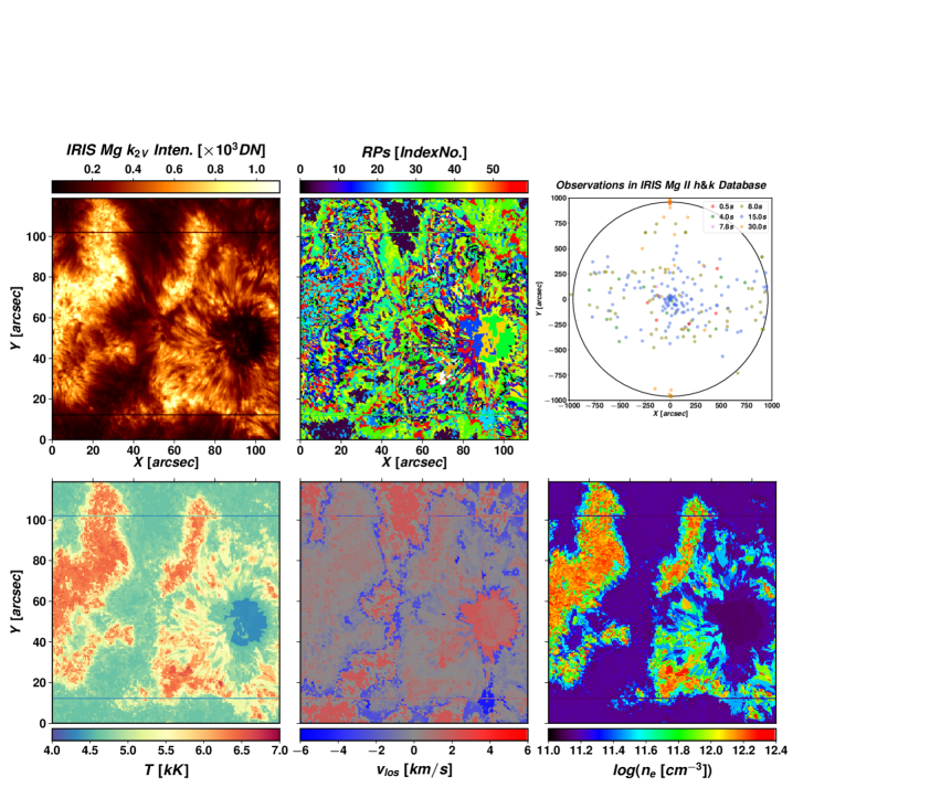
The left panel of the top row of Figure 1 shows the IRIS intensity map at the blue peak of Mg II $k$ line ($k_{2V}$ spectral feature) for NOAA AR 12480. In the central panel, the spatial distribution of the corresponding Mg II h&k RPs is shown. There, we can appreciate how the RPs are distributed in coherent patches in the spatio-temporal (since the raster scan takes time) domain. The second row of Figure 1 shows $T$, $v_{los}$, and $log(n_{e})$ recovered from the inversion of the RPs, i.e. in the RMAs of that dataset.

We call this method inversion of RPs by STiC or $\mathbf{RPs@STiC}$. Because we are inverting a reduced number of profiles (the RPs), this method can provide valuable information of the physical conditions in the IRIS field of view (FoV) within a few CPU hours.

The $RPs@STiC$ is a good method to recover information on spatially coherently averaged areas, although there is a loss of spatial information. Moreover, a few poorly fitted RPs may affect a large region. Thus, in the $v_{los}$ shown in Figure 1, the patches associated with the border between plage and quiet Sun show suspicious values. A close inspection of the quality of the fit of those RPs confirms that their match is not good. To avoid these flaws we have developed two more sophisticated methods.

2.2. Building the database

We have considered most of the main solar features observed in the photosphere and chromosphere. In addition, the employed data sets were selected considering position on the solar disk, exposure time, and IRIS observing modes: dense (0.33″steps) or sparse (1″) raster, and sit-and-stare. The location of all datasets included in the database is indicated in Figure 1.

The database consists of three elements: 15,000 observed RPs, the corresponding 15,000 synthetic RPs (from the inversion of the RPs), and the corresponding 15,000 model atmospheres. Because we have a large number of RPs, both the synthetic RPs and RMAs represent the variety of typical solar conditions quite well.

Our database is constructed from observations that are sensitive to the upper photosphere and chromosphere. Therefore, the IRIS Mg II h&k database may also be useful beyond the direct purpose of this paper. For instance, theoretical models and numerical simulations may find valuable observational constraints in our database.

3. Inversion of IRIS Mg II h&k lines based on inverted RPs

For any pixel of a given observation, e.g., the one shown in Figure 1, we look for the closest synthetic profile obtained by the StiC inversion of the RP in the IRIS Mg II h&k database ($I_{i}^{syn\ RP@STiC}$). To determine the closest profile we use the same loss function as in STiC,

$$\chi^{2}=\frac{1}{\nu}\sum_{i=0}^{q}{(I(\lambda_{i})^{obs}-I(\lambda_{i},\mathbf{M})^{syn\ RP@STiC})^{2}\frac{w_{i}^{2}}{\sigma_{i}^{2}}}$$ (1)

with $i=0,...,q$ the sampled wavelengths, $w_{i}$ their weights, $\sigma_{i}$ the uncertainties of the observation (e.g. photon noise), and $\nu$ the number of observables, i.e. , the spectral samples. A low value of $\chi^{2}$ tells us whether the fit between the observed ($I_{obs}$) and synthetic profiles $I_{i}^{syn\ RP@STiC}$ is good. We explicitly denote the dependency of the synthetic RP on the parameters of the model atmosphere ($\mathbf{M}$). Once the code has found the best match between the observed profile and a synthetic RP in the IRIS database, it associates the corresponding RMA of that (closest) synthetic RP to the pixel in our observation. For large datasets, this look-up table process may take a few minutes on a desktop machine. Then, the code provides a $\chi^{2}$-map (to indicate the goodness of the match between the observed and synthetic profiles in the database), the output model atmosphere, and the associated uncertainty of each variable of the model.

The uncertainty of a physical quantity $p$ is calculated following Eq. 42 in del Toro Iniesta & Ruiz Cobo (2016):

$$\sigma^{2}_{p}=\frac{2}{nm+r}\frac{\sum_{i=1}^{q}{\left[I(\lambda_{i})^{obs}-I(\lambda_{i};\mathbf{M})^{syn\ RP@STiC})^{2}\right]\frac{w_{i}^{2}}{\sigma_{i}^{2}}}}{\sum_{i=1}^{q}R^{2}_{p}(\lambda_{i})\frac{w_{i}^{2}}{\sigma_{i}^{2}}}$$ (2)

with $m$ the number of physical quantities in the model $\mathbf{M}$ evaluated in $n$ grid points along the solar atmosphere, $r$ the number of physical quantities considered constant along that atmosphere, and $R_{p}$ the Response Function (RF) of a Stokes parameter to the physical quantity $p$ (Mein, 1971; Landi Degl’Innocenti, 1979; Ruiz Cobo & del Toro Iniesta, 1992). The RF provides the sensitivity of a wavelength sample in a Stokes profile to (changes of) a physical quantity. Thus, we use expressions like: “The core of the Mg II h&k lines is sensitive to the $T$ in optical depths around $log(\tau)=-5$, while the wings are sensitive to $T$ in $-5<log(\tau)<-1$”.

We note that the inversion code does not operate over every grid point of the atmosphere, but over the nodes (each of them usually affect several grid points simultaneously). Therefore, in the latter case the RF is usually larger as a larger section of the atmosphere is perturbed per node and the uncertainty becomes lower than the estimates obtained by perturbing each grid point.

We have named this new tool the IRIS Inversion based on Representative Profiles Inverted by STiC or just IRIS squared ($\mathbf{IRIS^{2}}$).

Figure 1.— Top: Left: slit-reconstructed intensity map of NOAA AR 12480 observed by IRIS at Mg II $k_{2V}$. Center: location of the representative profiles (RPs). Right: location on the solar disk of the IRIS Mg II h&k database observations and their (color-encoded) exposure time. Bottom: from left to right, $T$, $v_{los}$, and electron density ($log(n_{e})$) evaluated at $log(\tau)=-4$.

$IRIS^{2}$ relies on two fundamental concepts: i) the relationship between the synthetic RPs and the RMAs, given by the inversion of the observed RPs by STiC, and ii) because the IRIS database covers a large variety of solar features, the RPs and corresponding RMAs are a meaningful representation of the variety found in the chromosphere and upper photosphere.

4. Inversion of IRIS Mg II h&k lines using deep learning

Since the IRIS Mg II h&k database includes synthetic profiles of the RPs and the corresponding RMAs, we have trained several deep neural networks (DNN) to reproduce this relationship. In deep learning jargon, a synthetic RP is the input layer, i.e., the intensities of the synthetic RP at the sampled wavelengths are the input nodes (473). The corresponding RMA is the output layer, i.e., the values of a physical quantities along the atmosphere (39) are the output nodes. Once the DNN is trained, we are , in principle, able to predict the physical quantity through the atmosphere for a given IRIS Mg II h&k profile.

We have considered $T$, $v_{los}$, $v_{turb}$, and $n_{e}$ as independent variables with respect to the corresponding synthetic RP. That means, we have trained a DNN for each of these physical quantities. The DNNs have different topologies (number of hidden layers and nodes), loss functions, and dropout parameters (to avoid overfitting). All the DNNs we have built use a rectified linear unit (ReLU) as activation functions, and we use 80% of the IRIS Mg II h&k database as a training set, and the remaining as a test set. Similarly, we have trained the uncertainties (along the atmosphere) of these physical quantities.

We have named this method deep IRIS squared or $\mathbf{deepIRIS^{2}}$. More detailed information about the used DNNs will be given in a follow-up paper.

5. Validation and Discussion

To validate $RPs@STiC$, $IRIS^{2}$, and $deepIRIS^{2}$, we have inverted, with STiC, every other pixel of the IRIS Mg II h&k observation of NOAA AR12480 on January 14, 2016. We consider the STiC results as the ground truth, but we should note that the STiC results also depend on initialization and are not guaranteed to provide a global minimum of the loss function.

Some results of using $RPs@STiC$ method are shown in the bottom of Figure 1. The first row of Figure 2 shows $T$ at $\log(\tau)=-4$ as result of the inversion using STiC (left), $IRIS^{2}$ (center), and $deepIRIS^{2}$ (right). Figure 3 shows $v_{los}$ (top), $v_{turb}$ (middle), and $log(n_{e})$ (bottom). Movies showing the variation of these parameters as a function of depth in the atmosphere are available in the electronic version.

5.1. Discussion: the reliable uncertainty range

One question we should answer to validate our results is: for a physical quantity at a given optical depth $p(\tau)$, how large is the unsigned difference between the value recovered by our method and the one obtained by STiC compared to the uncertainty estimated using Eq. 2? We define the Uncertainty Multiplication Factor (UMF) as:

$$UMF_{p}\ (\tau)=\frac{|p^{method}(\tau)-p^{STiC}(\tau)|}{\sigma_{p}^{STiC}(\tau)}$$ (3)

We have selected 5 regions of interest (RoIs) of $21^{\prime\prime}\times 21^{\prime\prime}$ in the FoV: plage (PL), quiet Sun (QS), umbra (UM), superpenumbra (SP), and a mix of regions (Mix, see Figure 2) to help us in the interpretation of the results. The full FoV (FFoV) is also evaluated.

The uncertainty maps ($\sigma$-maps) of $T$ obtained by STiC, $IRIS^{2}$  and $deepIRIS^{2}$ are shown in the second row of Figure 2. The first panel of the third row shows the $\chi^{2}$ map for STiC. The other panels in the third row show the $UMF$ for $T$ using the $IRIS^{2}$ (center) and $deepIRIS^{2}$ (right) methods. We have intentionally selected the optical depth $log(\tau)=-4$ because it illustrates several key issues.

Figure 2.— Top: First row: $T$ for NOAA AR 12480 at $log(\tau)=-4$ provided by STiC (left), $IRIS^{2}$ (center), and $deepIRIS^{2}$ (right). Middle: uncertainties for these methods. Bottom Left: $\chi^{2}$-map associated to STiC results. Center and right: uncertainty multiplication factor ($UMF_{T}$) for $IRIS^{2}$ and $deepIRIS^{2}$ methods. Regions of interest (RoIs) are marked with squares in the center panel of the top row.

Figure 3.— Some thermodynamic quantities recovered by STiC (left), $IRIS^{2}$ (center), and $deepIRIS^{2}$ (right) at $log(\tau)=-4$: $v_{los}$ (top), $v_{turb}$ (middle), and $log(n_{e})$ (bottom).

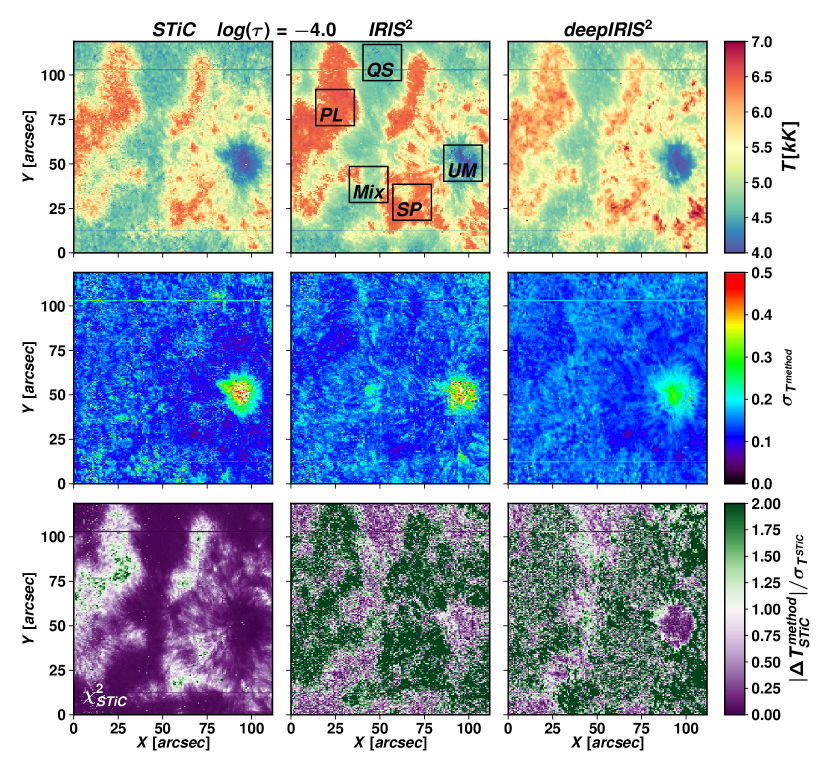
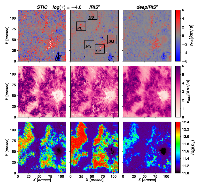
Some regions in the $\sigma$-maps are better (lower values) for $IRIS^{2}$ and $deepIRIS^{2}$ than for STiC. This is a direct consequence of the better fit obtained by $IRIS^{2}$ compared to STiC, as mentioned above. The $\chi^{2}$ map shown in the bottom-left panel of Figure 2 is normalized in such a way that: the fit is bad in regions where $\chi^{2}\gg 1$, indicating that $p(\tau)$ is likely suffering from large uncertainties or may be wrong; the fits are better/good in regions with $\chi^{2}$ of order 1 or less. In the $UMF_{p}$-maps (bottom center and right panels of Figure 2) regions with $UMF_{p}$$\approx 1$ have values of $p(\tau)$ as ”accurate” as STiC, or even better if $UMF_{p}$$\ll 1$. Our example at $log(\tau)=-4$ indicates that care should be taken when interpreting the results in plage and the superpenumbra.

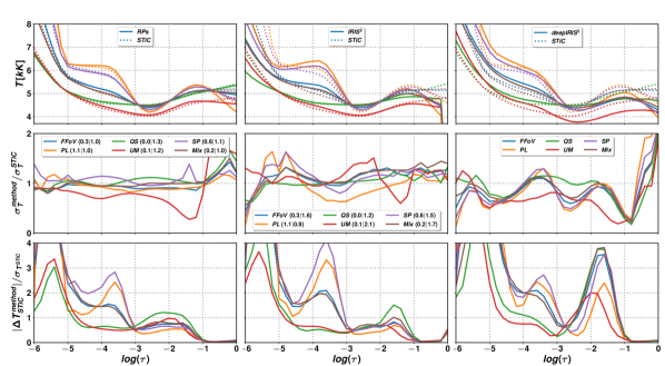
Figure 4 shows the behavior of $T^{method}$ and $T^{STiC}$ (in thick and dashed line respectively in the first row), the ratio between the uncertainties ($\sigma^{method}_{T}/\sigma^{STiC}_{T}$, second row), and the $UMF_{p}$ (third row) for the proposed methods. The numbers next to the RoIs labels in the legend are the spatially-averaged normalized $\chi^{2}_{STiC}$ and the ratio $\chi^{2}_{method}/\chi^{2}_{STiC}$.

The uncertainties ratios show that mostly all the methods show the same uncertainty as STiC. In some regions the other methods give better results, in other cases the opposite is true, but on average (blue line) the behavior is very similar, or clearly better.

The $UMF_{p}$ for $RPs@STiC$ and $IRIS^{2}$ is $\lesssim 1$ in all RoIs for $-3.5<log(\tau)<-1$. For plage, the UMF for $-4.5<log(\tau)<-3$ is $\lesssim 1$, and $\chi^{2}_{method}\leq\chi^{2}_{STiC}$, therefore the values provided by these methods are more accurate than the ones from STiC. The situation is the opposite for the superpenumbra. All in all, the values provided by $RPs@STiC$ and $IRIS^{2}$ are mostly valid where Mg II h&k lines are sensitive to $T$, i.e. $-5<log(\tau)<-1$. For $deepIRIS^{2}$, we have to be cautious, even when the uncertainties ratio is $\lesssim 1$ in all the RoIs, the difference in $T$ is noticeable in some of the ROIs.

Figure 5 shows the $UMF_{p}$ for $v_{los}$, $v_{turb}$, and $log(n_{e})$. All the methods have a similar behavior in all the RoIs for $v_{los}$ and $v_{turb}$, but there are differences for $log(n_{e})$ in plage regions for the $IRIS^{2}$ and $deepIRIS^{2}$methods. We note that that while substantial differences of physical parameters between different methods can occur, these differences may often be smaller than the intrinsic uncertainty.

Figure 4.— For the full FoV (FFOV, blue line) and the RoIs framed in Figure 2: Top: $T$ along the optical depth in the atmosphere ($log(\tau)$) for STiC (dashed line), $RPs@STiC$ (left), $IRIS^{2}$ (center), and $deepIRIS^{2}$ (right). Middle: ratio between the uncertainty of the new methods with respect to the uncertainty of STiC.  Bottom: uncertainty multiplication factor ($UMF_{T}$) for the new methods (see Eq. 3)

.

Figure 5.— Uncertainty multiplication factor ($UMF_{p}$, see Eq. 3) for $v_{los}$ (top), $v_{turb}$ (center), and $n_{e}$ (right) for the new methods for the full FoV (FFOV, blue line) and the RoIs framed in Figure 2.

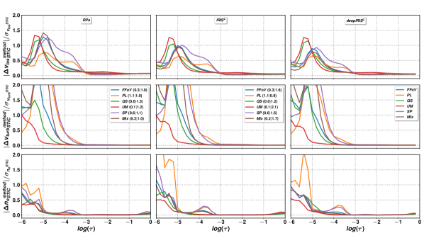
In summary, any of the proposed methods provides these values as well ast STiC – or even better –, within the intrinsic uncertainties. However, when we interpret a physical quantity and its uncertainty provided by our methods we should be specially cautious in: i) regions showing large values in the $\chi^{2}$-map, i.e. where the fit between the observed profiles and the synthetic profiles is not good, and ii) those optical depths where Mg II h&k lines are less sensitive to variations of a physical parameter. Under those conditions, the uncertainty will be larger, e.g., 2 or 3 times larger than the uncertainties provided in the database (as the UMF values in Fig. 2 and 3 suggest).

6. Conclusions

We have created and evaluated three novel methods to rapidly obtain the atmospheric physical quantities in the chromosphere and upper photosphere from the profiles of the IRIS Mg II h&k lines. The methods presented are valid for any spectro(polarimetric) data as far as they can be inverted by a traditional inversion code. We note that $IRIS^{2}$ can be used for any IRIS observation that includes Mg II h or Mg II k (or both) lines.

We summarize the main advantages and disadvantages for the three methods:

• $RPs@STiC$: on average, it is the closest to STiC. However, we lose spatial information. This can be minimized by using a much larger number of RPs for each dataset. It stills requires a proper inversion, which takes hundreds of CPU-hours (e.g. 320 CPU-hours for 160 RPs).

• $IRIS^{2}$: it offers results as good as STiC on average, being slightly better or worse than the latter in some solar features. The spatial information is almost as good as the original, although some regions may show little variation if the profiles are associated with the same RP in the database. That can be minimized by including a larger variety of profiles in the database. This method is $10^{5}-10^{6}$ times faster than STiC.

• $deepIRIS^{2}$: it predicts values of $v_{vlos}$, $v_{turb}$, and $n_{e}$, as good as the ones obtained by STiC. The predicted values for $T$ are not as good but acceptable. A more complex DNN architecture and larger training and test datasets can improve this. The results do not lose spatial information and they look spatially smooth. It is $\approx 10^{6}$ times faster than STiC.

As a result of our investigation, we conclude that $IRIS^{2}$ is currently the fastest, easy-to-use method to recover reliable information from the chromosphere and photosphere from IRIS Mg II h&k data. While we are improving these methods with a new database that includes 160 RPs per dataset, as well as more observations, we note that the current versions of IRIS Mg II h&k lines database, $IRIS^{2}$(both in IDL and Python), and $deepIRIS^{2}$ are available to the community at http://iris.lmsal.com/analysis.html. We expect that our database can be applied to a wide variety of investigations that use IRIS data.

This work is supported by NASA under contract NNG09FA40C (IRIS) and the Lockheed Martin Independent Research Program. JdlCR is supported by grants from the Swedish Research Council (2015-03994), the Swedish National Space Board (128/15) and the Swedish Civil Contingencies Agency (MSB). This project has received funding from the European Research Council (ERC) under the European Union’s Horizon 2020 research and innovation programme (SUNMAG, grant agreement 759548). This paper has benefited from discussions at a meeting of team 399 ’Studying magnetic-field-regulated heating in the solar chromosphere’ at the International Space Science Institute (ISSI) in Switzerland. IRIS is a NASA small explorer mission developed and operated by LMSAL with mission operations executed at NASA Ames Research center and major contributions to downlink communications funded by ESA and the Norwegian Space Centre.

References

- de la Cruz Rodríguez et al. (2016) de la Cruz Rodríguez, J., Leenaarts, J., & Asensio Ramos, A. 2016, ApJ, 830, L30
- de la Cruz Rodríguez et al. (2018) de la Cruz Rodríguez, J., Leenaarts, J., Danilovic, S., & Uitenbroek, H. 2018, arXiv:1810.08441
- De Pontieu et al. (2014) De Pontieu, B., Title, A. M., Lemen, J. R., et al. 2014, Sol. Phys., 289, 2733
- del Pino Alemán et al. (2016) del Pino Alemán, T., Casini, R., & Manso Sainz, R. 2016, ApJ, 830, L24
- del Toro Iniesta & Ruiz Cobo (2016) del Toro Iniesta, J. C., & Ruiz Cobo, B. 2016, Living Reviews in Solar Physics, 13, 4
- Landi Degl’Innocenti (1979) Landi Degl’Innocenti, E. 1979, Sol. Phys., 63, 237
- Leenaarts et al. (2013a) Leenaarts, J., Pereira, T. M. D., Carlsson, M., Uitenbroek, H., & De Pontieu, B. 2013a, ApJ, 772, 89
- Leenaarts et al. (2013b) —. 2013b, ApJ, 772, 90
- MacQueen (1967) MacQueen, J. 1967, in Fifth Berkeley Sympos. Math. Statist. and Probability. I: Statistics, ed. C. University California Press, Berkeley, 281
- Mein (1971) Mein, P. 1971, Sol. Phys., 20, 3
- Pereira et al. (2015) Pereira, T. M. D., Carlsson, M., De Pontieu, B., & Hansteen, V. 2015, ApJ, 806, 14
- Ruiz Cobo & del Toro Iniesta (1992) Ruiz Cobo, B., & del Toro Iniesta, J. C. 1992, ApJ, 398, 375
- Steinhaus (1957) Steinhaus, H. 1957, Bull. Acad. Polon. Sci., 4, 801
- Sukhorukov & Leenaarts (2017) Sukhorukov, A. V., & Leenaarts, J. 2017, A&A, 597, A46