Decoupled Data Based Approach for Learning to Control Nonlinear Dynamical Systems

Abstract

This paper addresses the problem of learning the optimal control policy for a nonlinear stochastic dynamical system with continuous state space, continuous action space and unknown dynamics. This class of problems are typically addressed in stochastic adaptive control and reinforcement learning literature using model-based and model-free approaches respectively. Both methods rely on solving a dynamic programming problem, either directly or indirectly, for finding the optimal closed loop control policy. The inherent ‘curse of dimensionality’ associated with dynamic programming method makes these approaches also computationally difficult.

This paper proposes a novel decoupled data-based control (D2C) algorithm that addresses this problem using a decoupled, ‘open loop - closed loop’, approach. First, an open-loop deterministic trajectory optimization problem is solved using a black-box simulation model of the dynamical system. Then, a closed loop control is developed around this open loop trajectory by linearization of the dynamics about this nominal trajectory. By virtue of linearization, a linear quadratic regulator based algorithm can be used for this closed loop control. We show that the performance of D2C algorithm is approximately optimal. Moreover, simulation performance suggests significant reduction in training time compared to other state of the art algorithms.

I Introduction

Controlling an unknown dynamical system adaptively has a rich history in control literature [1] [2]. These classical literature provides rigorous analysis about the asymptotic performance and stability of the closed loop system. Classical adaptive control literature mainly focuses on non-stochastic systems [3] [4]. Stochastic adaptive control literature mostly addresses tractable models like linear quadratic regulator (LQR) where Riccati equation based closed form expressions are available for the optimal control law. Optimal control of an unknown nonlinear dynamical system with continuous state space and continuous action space is a significantly more challenging problem. Even with a known model, computing an optimal control law requires solving a dynamic programming problem. The ‘curse of dimensionality’ associated with dynamic programming makes solving such problems computationally intractable, except under special structural assumptions on the underlying system. Learning to control problems where the model of the system is unknown also suffer from this computational complexity issues, in addition to the usual identifiability problems in adaptive control.

Last few years have seen significant progresses in deep neural netwoks based reinforcement learning approaches for controlling unknown dynamical systems, with applications in many areas like playing games [5], locomotion [6] and robotic hand manipulation [7]. A number of new algorithms that show promising performance are proposed [8] [9] [10] and various improvements and innovations have been continuously developed. However, despite excellent performance on a number of tasks, reinforcement learning (RL) is still considered very data intensive. The training time for such algorithms are typically really large. Moreover, high variance and reproducibility issues on the performance are also reported [11]. While there have been some attempts to improve the sample efficiency [12], a systematic approach is still lacking.

In this work, we propose a novel decoupled data based control (D2C) algorithm for learning to control an unknown nonlinear dynamical system. Our approach introduces a rigorous decoupling of the open loop (planning) problem from the closed loop (feedback control) problem. This decoupling allows us to come up with a highly sample efficient approach to solve the problem in a completely data based fashion. Our approach proceeds in two steps: (i) first, we optimize the nominal open loop trajectory of the system using a blackbox simulation model, (ii) then we identify the linear system governing perturbations from the nominal trajectory using random input-output perturbation data, and design an LQR controller for this linearized system. We show that the performance of D2C algorithm is approximately optimal, in the sense that the decoupled design is near optimal to second order in a suitably defined noise parameter. Moreover, simulation performance suggests significant reduction in training time compared to other state of the art algorithms.

Related works: The solution approaches to the problem of controlling an unknown dynamical systems can be divided into two broad classes, model-based methods and model-free methods.

In the model-based methods, many techniques [13] rely on a discretization of the underlying state and action space, and hence, run into the curse of dimensionality, the fact that the computational complexity grows exponentially with the dimension of the state space of the problem. The most computationally efficient among these techniques are trajectory-based methods such as differential dynamic programming (DDP) [14] [15] which linearizes the dynamics and the cost-to-go function around a given nominal trajectory, and designs a local feedback controller using DP. The iterative linear quadratic Gaussian (ILQG) [16] [17], which is closely related to DDP, considers the first order expansion of the dynamics (in DDP, a second order expansion is considered), and designs the feedback controller using Riccati-like equations, and is shown to be computationally more efficient. In both approaches, the control policy is executed to compute a new nominal trajectory, and the procedure is repeated until convergence.

Model-free methods, more popularly known as approximate dynamic programming [18] [19] or reinforcement learning (RL) methods [20], seek to improve the control policy by repeated interactions with the environment, while observing the system’s responses. The repeated interactions, or learning trials, allow these algorithms to compute the solution of the dynamic programming problem (optimal value/Q-value function or optimal policy) without explicitly constructing the model of the unknown dynamical system. Standard RL algorithms are broadly divided into value-based methods, like Q-learning, and policy-based methods, like policy gradient algorithms. Recently, function approximation using deep neural networks has significantly improved the performance of reinforcement learning algorithm, leading to a growing class of literature on ‘deep reinforcement learning’. Despite the success, the amount of samples and training time required still seem prohibitive.

Our Contributions: Rather than directly finding the closed loop control law which requires solving a dynamic programming problem, our approach addresses the original stochastic control problem in a ’decoupled open loop - closed loop’ fashion. In this approach: i) we solve an open loop deterministic optimization problem to obtain an optimal nominal trajectory in a model-free fashion, and then ii) we design a closed loop controller for the resulting linearized time-varying system around the optimal nominal trajectory, in a model-based fashion. This ‘divide and conquer’ strategy can be shown to be extremely effective. In this context, our major contributions are: 1) we show a near optimal parametrization of the feedback policy in terms of an open loop control sequence, and a linear feedback control law, 2) we show rigorously that the open loop and closed loop learning can be decoupled, which 3) results in the D2C algorithm that is highly data efficient when compared to state of the art RL techniques. This paper is a rigorous extension of our preliminary work [21, 22], in particular, it includes a stronger decoupling result, and an extensive empirical evaluation of the D2C algorithm with state of the art RL implementations on standard benchmark problems.

The rest of the paper is organized as follows. In Section II, the basic problem formulation is outlined. In Section III, a decoupling result which solves the MDP in a “decoupled open loop-closed loop ” fashion is briefly summarized. In Section IV, we propose a decoupled data based control algorithm, with discussions of implementation problems. In Section V, we test the proposed approach using four typical benchmarking examples with comparisons to a state of the art RL technique.

II PROBLEM FORMULATION

Consider the following discrete time nonlinear stochastic dynamical system:

$$x_{t+1}=h(x_{t},u_{t},w_{t}),$$ (1)

where $x_{t}\in\mathbb{R}^{n_{x}}$, $u_{t}\in\mathbb{R}^{n_{u}}$ are the state measurement and control vector at time $k$, respectively. The process noise $w_{t}$ is assumed as zero-mean, uncorrelated Gaussian white noise, with covariance $W$.

The optimal stochastic control problem is to find the the control policy $\pi^{o}=\{\pi^{o}_{1},\pi^{o}_{2},\cdots,\pi^{o}_{T-1}\}$ such that the expected cumulative cost is minimized, i.e.,

$$\pi^{o} =\arg\min_{\pi}~{}\tilde{J}^{\pi}(x),~{}~{}\text{where,}$$

$$\tilde{J}^{\pi}(x) =\mathbb{E}_{\pi}\left[\sum_{t=1}^{T-1}c(x_{t},u_{t})+c_{T}(x_{T})|x_{1}=x\right],$$ (2)

$u_{t}=\pi_{t}(x_{t})$, $c(\cdot,\cdot)$ is the instantaneous cost function, and $c_{T}(\cdot)$ is the terminal cost function. In the following, we assume that the initial state $x_{1}$ is fixed, and denote $\tilde{J}^{\pi}(x)$ simply as $\tilde{J}^{\pi}$.

If the function $h(\cdot,\cdot,\cdot)$ is known exactly, then the optimal control law $\pi^{o}$ can be computed using dynamic programming method. However, as noted before, this can be often computationally intractable. Moreover, when $h$ is unknown, designing an optimal closed loop control law is a much more challenging problem. In the following, we propose a data based decoupled approach for solving (II) when $h$ is unknown.

III A NEAR OPTIMAL DECOUPLING PRINCIPLE

We first outline a near-optimal decoupling principle in stochastic optimal control that paves the way for the D2C algorithm described in Section IV.

We make the following assumptions for the simplicity of illustration. We assume that the dynamics given in (1) can be written in the form

$$x_{t+1}=f(x_{t})+B_{t}(u_{t}+\epsilon w_{t}),$$ (3)

where $\epsilon<1$ is a small parameter. We also assume that the instantaneous cost $c(\cdot,\cdot)$ has the following simple form,

$$c(x,u)=l(x)+\frac{1}{2}u^{\prime}Ru.$$ (4)

We emphasis that these assumptions, quadratic control cost and affine in control dynamics, are purely for the simplicity of treatment. These assumptions can be omitted at the cost of increased notational complexity.

III-A Linearization w.r.t. Nominal Trajectory

Consider a noiseless version of the system dynamics given by (3). We denote the “nominal” state trajectory as $\bar{x}_{t}$ and the “nominal” control as $\bar{u}_{t}$ where $u_{t}=\pi_{t}(x_{t})$, where $\pi=(\pi_{t})^{T-1}_{t=1}$ is a given control policy. The resulting dynamics without noise is given by $\bar{x}_{t+1}=f(\bar{x}_{t})+B_{t}\bar{u}_{t}$.

Assuming that $f(\cdot)$ and $\pi_{t}(\cdot)$ are sufficiently smooth, we can linearize the dynamics about the nominal trajectory. Denoting $\delta x_{t}=x_{t}-\bar{x}_{t},\delta u_{t}=u_{t}-\bar{u}_{t}$, we can express,

$$\delta x_{t+1} =A_{t}\delta x_{t}+B_{t}\delta u_{t}+S_{t}(\delta x_{t})+\epsilon w_{t},$$ (5)

$$\delta u_{t} =K_{t}\delta x_{t}+\tilde{S}_{t}(\delta x_{t}),$$ (6)

where $A_{t}=\frac{\partial f}{\partial x}|_{\bar{x}_{t}}$, $K_{t}=\frac{\partial\pi_{t}}{\partial x}|_{\bar{x}_{t}}$, and $S_{t}(\cdot),\tilde{S}_{t}(\cdot)$ are second and higher order terms in the respective expansions. Similarly, we can linearize the instantaneous cost $c(x_{t},u_{t})$ about the nominal values $(\bar{x}_{t},\bar{u}_{t})$ as,

$$c(x_{t},u_{t}) ={l}(\bar{x}_{t})+L_{t}\delta x_{t}+H_{t}(\delta x_{t})+$$

$$\hskip 28.45274pt\frac{1}{2}\bar{u}_{t}^{\prime}R\bar{u}_{t}+\delta u_{t}^{\prime}R\bar{u}_{t}+\delta u_{t}^{\prime}R\delta u_{t},$$ (7)

$$c_{T}(x_{T}) ={c}_{T}(\bar{x}_{T})+C_{T}\delta x_{T}+H_{T}(\delta x_{T}),$$ (8)

where $L_{t}=\frac{\partial l}{\partial x}|_{\bar{x}_{t}}$, $C_{T}=\frac{\partial c_{T}}{\partial x}|_{\bar{x}_{t}}$, and $H_{t}(\cdot)$ and $H_{T}(\cdot)$ are second and higher order terms in the respective expansions.

Using (5) and (6), we can write the closed loop dynamics of the trajectory $(\delta x_{t})^{T}_{t=1}$ as,

$$\delta x_{t+1}=\underbrace{(A_{t}+B_{t}K_{t})}_{\bar{A}_{t}}\delta x_{t}+\underbrace{\{B_{t}\tilde{S}_{t}(\delta x_{t})+S_{t}(\delta x_{t})\}}_{\bar{S}_{t}(\delta x_{t})}+\epsilon w_{t},$$ (9)

where $\bar{A}_{t}$ represents the linear part of the closed loop systems and the term $\bar{S}_{t}(.)$ represents the second and higher order terms in the closed loop system. Similarly, the closed loop incremental cost given in (7) can be expressed as

$$c(x_{t},u_{t})=\underbrace{\{{l}(\bar{x}_{t})+\frac{1}{2}\bar{u}_{t}^{\prime}R\bar{u}_{t}\}}_{\bar{c}_{t}}+\underbrace{[L_{t}+\bar{u}_{t}^{\prime}RK_{t}]}_{\bar{C}_{t}}\delta x_{t}$$

$$+\underbrace{(K_{t}\delta x_{t}+\tilde{S}_{t}(\delta x_{t}))^{\prime}R(K_{t}\delta x_{t}+\tilde{S}_{t}(\delta x_{t}))}_{\bar{H}_{t}(\delta x_{t})}.$$ (10)

Therefore, the cumulative cost of any given closed loop trajectory $(x_{t},u_{t})^{T}_{t=1}$ can be expressed as,

$$J^{\pi} =\sum^{T-1}_{t=1}c(x_{t},u_{t}=\pi_{t}(x_{t}))+c_{T}(x_{T})$$

$$=\sum_{t=1}^{T}\bar{c}_{t}+\sum_{t=1}^{T}\bar{C}_{t}\delta x_{t}+\sum_{t=1}^{T}\bar{H}_{t}(\delta x_{t}),$$ (11)

where $\bar{c}_{T}=c_{T}(\bar{x}_{T}),\bar{C}_{T}=C_{T}$.

We first show the following result.

Lemma 1

The state perturbation equation

$$\delta x_{t+1}=\bar{A}_{t}\delta x_{t}+\bar{S}_{t}(\delta x_{t})+\epsilon w_{t}$$

given in (9) can be equivalently characterized as

$$\delta x_{t}=\delta x_{t}^{l}+\bar{\bar{S_{t}}},~{}\delta x_{t+1}^{l}=\bar{A}_{t}\delta x_{t}^{l}+\epsilon w_{t}$$ (12)

where $\bar{\bar{S}}_{t}$ is an $O(\epsilon^{2})$ function that depends on the entire noise history $\{w_{0},w_{1},\cdots w_{t}\}$ and $\delta x_{t}^{l}$ evolves according to the linear closed loop system.

Proof is omitted due to page limits. Detailed proof is given in [23].

Using (12) in (III-A), we can obtain the cumulative cost of any given closed loop trajectory as,

$$J^{\pi}=\underbrace{\sum_{t=1}^{T}\bar{c}_{t}}_{\bar{J}^{\pi}}+\underbrace{\sum_{t=1}^{T}\bar{C}_{t}\delta x_{t}^{l}}_{\delta J_{1}^{\pi}}+\underbrace{\sum_{t=1}^{T}\bar{H}_{t}(\delta x_{t})+\bar{C}_{t}\bar{\bar{S}}_{t}}_{\delta J_{2}^{\pi}}.$$ (13)

Now, we show the following important result.

Proposition 1

$$\tilde{J}^{\pi} =\mathbb{E}[J^{\pi}]=\bar{J}^{\pi}+O(\epsilon^{2}),$$

$$\text{Var}(J^{\pi}) =\underbrace{\text{Var}(\delta J_{1}^{\pi})}_{O(\epsilon^{2})}+O(\epsilon^{4}).$$

Proof:

From (13), we get,

$$\tilde{J}^{\pi}=\mathbb{E}[J^{\pi}]=\mathbb{E}[\bar{J}^{\pi}+\delta J_{1}^{\pi}+\delta J_{2}^{\pi}],$$

$$=\bar{J}^{\pi}+\mathbb{E}[\delta J_{2}^{\pi}]=\bar{J}^{\pi}+O(\epsilon^{2}),$$ (14)

The first equality in the last line of the equations before follows from the fact that $\mathbb{E}[\delta x_{t}^{l}]=0$, since its the linear part of the state perturbation driven by white noise and by definition $\delta x_{1}^{l}=0$.The second equality follows form the fact that $\delta J_{2}^{\pi}$ is an $O(\epsilon^{2})$ function. Now,

$$\text{Var}(J^{\pi})=\mathbb{E}[J^{\pi}-\tilde{J}^{\pi}]^{2}$$

$$=\mathbb{E}[\bar{J}_{0}^{\pi}+\delta J_{1}^{\pi}+\delta J_{2}^{\pi}-\bar{J}_{0}^{\pi}-\delta\tilde{J}_{2}^{\pi}]^{2}$$

$$=\text{Var}(\delta J_{1}^{\pi})+\text{Var}(\delta J_{2}^{\pi})+2\mathbb{E}[\delta J_{1}^{\pi}\delta J_{2}^{\pi}].$$ (15)

Since $\delta J_{2}^{\pi}$ is $O(\epsilon^{2})$, $\text{Var}(\delta J_{2}^{\pi})$ is an $O(\epsilon^{4})$ function. It can be shown that $\mathbb{E}[\delta J_{1}^{\pi}\delta J_{2}^{\pi}]$ is $O(\epsilon^{4})$ as well (proof is given [23]). Finally $\text{Var}(\delta J_{1}^{\pi})$ is an $O(\epsilon^{2})$ function because $\delta x^{l}$ is an $O(\epsilon)$ function. Combining these, we will get the desired result. ∎

The following observations can now be made from Proposition 1.

Remark 1 (Expected cost-to-go)

Recall that $u_{t}=\pi_{t}(x_{t})$ $=\bar{u}_{t}+K_{t}\delta x_{t}+\tilde{S}_{t}(\delta x_{t})$. However, note that due to Proposition 1, the expected cost-to-go, $\tilde{J}^{\pi}$, is determined almost solely (within $O(\epsilon^{2})$) by the nominal control action sequence $\bar{u}_{t}$. In other words, the linear and higher order feedback terms have only $O(\epsilon^{2})$ effect on the expected cost-to-go function.

Remark 2 (Variance of cost-to-go)

Given the nominal control action $\bar{u}_{t}$, the variance of the cost-to-go, which is $O(\epsilon^{2})$, is determined overwhelmingly (within $O(\epsilon^{4})$) by the linear feedback term $K_{t}\delta x_{t}$, i.e., by the variance of the linear perturbation of the cost-to-go, $\delta J_{1}^{\pi}$, under the linear closed loop system $\delta x_{t+1}^{l}=(A_{t}+B_{t}K_{t})\delta x_{t}^{l}+\epsilon w_{t}$.

III-B Decoupled Approach for Closed Loop Control

Proposition 1 and the remarks above suggest that an open loop control super imposed with a closed loop control for the perturbed linear system may be approximately optimal. We delineate this idea below.

Open Loop Design. First, we design an optimal (open loop) control sequence $\bar{u}^{*}_{t}$ for the noiseless system. More precisely,

$$(\bar{u}^{*}_{t})^{T-1}_{t=1} =\arg\min_{(\tilde{u}_{t})^{T-1}_{t=1}}\sum_{t=1}^{T-1}c(\bar{x}_{t},\tilde{u}_{t})+c_{T}(\bar{x}_{T}),$$ (16)

$$\bar{x}_{t+1} =f(\bar{x}_{t})+B_{t}\tilde{u}_{t}.$$

We will discuss the details of this open loop design in Section IV.

Closed Loop Design. We find the optimal feedback gain $K^{*}_{t}$ such that the variance of the linear closed loop system around the nominal path, $(\bar{x}_{t},\bar{u}^{*}_{t})$, from the open loop design above, is minimized.

$$(K^{*}_{t})^{T-1}_{t=1} =\arg\min_{(K_{t})^{T-1}_{t=1}}~{}\text{Var}(\delta J_{1}^{\pi}),$$

$$\delta J_{1}^{\pi}=\sum_{t=1}^{T}\bar{C}_{t}x_{t}^{l},$$

$$\delta x_{t+1}^{l}=(A_{t}+B_{t}K_{t})\delta x_{t}^{l}+\epsilon w_{t}.$$ (17)

We now characterize the approximate closed loop policy below.

Proposition 2

Construct a closed loop policy

$$\pi_{t}^{*}(x_{t})=\bar{u}_{t}^{*}+K_{t}^{*}\delta x_{t},$$ (18)

where $\bar{u}_{t}^{*}$ is the solution of the open loop problem (16), and $K_{t}^{*}$ is the solution of the closed loop problem (17). Let $\pi^{o}$ be the optimal closed loop policy. Then,

$$|\tilde{J}^{\pi*}-\tilde{J}^{\pi^{o}}|=O(\epsilon^{2}).$$

Furthermore, among all policies with nominal control action $\bar{u}_{t}^{*}$, the variance of the cost-to-go under policy $\pi_{t}^{*}$, is within $O(\epsilon^{4})$ of the variance of the policy with the minimum variance.

Proof:

We have

$$\tilde{J}^{\pi^{*}}-\tilde{J}^{\pi^{o}} =\tilde{J}^{\pi^{*}}-\bar{J}^{\pi^{*}}+\bar{J}^{\pi^{*}}-\tilde{J}^{\pi^{o}}$$

$$\leq\tilde{J}^{\pi^{*}}-\bar{J}^{\pi^{*}}+\bar{J}^{\pi^{o}}-\tilde{J}^{\pi^{o}}$$

The inequality above is due the fact that $\bar{J}^{\pi^{*}}\leq\bar{J}^{\pi^{o}}$, by definition of $\pi^{*}$. Now, using Proposition 1, we have that $|\tilde{J}^{\pi^{*}}-\bar{J}^{\pi^{*}}|=O(\epsilon^{2})$, and $|\tilde{J}^{\pi^{o}}-\bar{J}^{\pi^{o}}|=O(\epsilon^{2})$. Also, by definition, we have $\tilde{J}^{\pi^{o}}\leq\tilde{J}^{\pi^{*}}$. Then, from the above inequality, we get

$$|\tilde{J}^{\pi^{*}}-\tilde{J}^{\pi^{o}}|\leq|\tilde{J}^{\pi^{*}}-\bar{J}^{\pi^{*}}|+|\bar{J}^{\pi^{o}}-\tilde{J}^{\pi^{o}}|=O(\epsilon^{2})$$

A similar argument holds for the variance as well. ∎

Unfortunately, there is no standard solution to the closed loop problem (17) due to the non additive nature of the cost function $\text{Var}(\delta J_{1}^{\pi})$. Therefore, we solve a standard LQR problem as a surrogate, and the effect is again one of reducing the variance of the cost-to-go by reducing the variance of the closed loop trajectories.

Approximate Closed Loop Problem. We solve the following LQR problem for suitably defined cost function weighting factors $Q_{t}$, $R_{t}$:

$$\min_{(\delta u_{t})^{T}_{t=1}}~{} \mathbb{E}[\sum_{t=1}^{T-1}\delta x_{t}^{\prime}Q_{t}\delta x_{t}+\delta u_{t}^{\prime}R_{t}\delta u_{t}+\delta x_{T}^{\prime}Q_{T}\delta x_{t}],$$

$$\delta x_{t+1}=A_{t}\delta x_{t}+B_{t}\delta u_{t}+\epsilon w_{t}.$$ (19)

The solution to the above problem furnishes us a feedback gan $\hat{K}_{t}^{*}$ which we can use in the place of the true variance minimizing gain $K_{t}^{*}$.

Remark 3

Proposition 1 states that the expected cost-to-go of the problem is dominated by the nominal cost-to-go. Therefore, even an open loop policy consisting of simply the nominal control action is within $O(\epsilon^{2})$ of the optimal expected cost-to-go. However, the plan with the optimal feedback gain $K_{t}^{*}$ is strictly better than the open loop plan in that it has a lower variance in terms of the cost to go. Furthermore, solving the approximate closed loop problem using the surrogate LQR problem, we can expect a lower variance of the cost-to-go function as well.

IV Decoupled Data Based Control (D2C) Algorithm

In this section, we propose a novel decoupled data based control (D2C) algorithm formalizing the ideas proposed in Section III. First, a noiseless open-loop optimization problem is solved to find a nominal optimal trajectory. Then a linearized closed-loop controller is designed around this nominal trajectory, such that, with existence of stochastic perturbations, the state stays close to the optimal open-loop trajectory. The three-step framework to solve the stochastic feedback control problem may be summarized as follows.

• Solve the open loop optimization problem using gradient decent with a black box simulation model of the dynamics.

• Linearize the system around the nominal open loop optimal trajectory, and identify the linearized time-varying system from input-output experiment data using a suitable system identification algorithm.

• Design an LQR controller which results in an optimal linear control policy around the nominal trajectory.

In the following section, we discuss each of the above steps.

IV-A Open Loop Trajectory Optimization

A first order gradient descent based algorithm is proposed here for solving the open loop optimization problem given in (16), where the underlying dynamic model is used as a blackbox, and the necessary gradients are found from a sequence of input perturbation experiment data using standard least square.

Denote the initial guess of the control sequence as $U^{(0)}=\{\bar{u}_{t}^{(0)}\}_{t=1}^{T}$, and the corresponding states $\mathcal{X}^{(0)}=\{\bar{x}_{t}^{(0)}\}_{t=1}^{T}$. The control policy is updated iteratively via

$$U^{(n+1)}=U^{(n)}-\alpha\nabla_{U}\bar{J}|_{\mathcal{X}^{(n)},U^{(n)}},$$ (20)

where $U^{(n)}=\{\bar{u}_{t}^{(n)}\}_{t=1}^{T}$ denotes the control sequence in the $n^{th}$ iteration, $\mathcal{X}^{(n)}=\{\bar{x}_{t}^{(n)}\}_{t=1}^{T}$ denotes the corresponding states, and $\alpha$ is the step size parameter. As $\bar{J}|_{\mathcal{X}^{(n)},U^{(n)}}$ is the expected cumulative cost under control sequence $U^{(n)}$ and corresponding states $\mathcal{X}^{(n)}$, the gradient vector is defined as

$$\nabla_{U}\bar{J}|_{\mathcal{X}^{(n)},U^{(n)}}=\begin{pmatrix}\frac{\partial\bar{J}}{\partial u_{1}}&\frac{\partial\bar{J}}{\partial u_{1}}&\cdots&\frac{\partial\bar{J}}{\partial u_{T}}\end{pmatrix}|_{\mathcal{X}^{(n)},U^{(n)}},$$ (21)

which is the gradient of the expected cumulative cost w.r.t the control sequence after $n$ iterations. The following paragraph elaborates on how to estimate the above gradient.

Let us define a rollout to be an episode in the simulation that starts from the initial settings to the end of the horizon with a control sequence. For each iteration, multiple rollouts are conducted sequentially with both the expected cumulative cost and the gradient vector updated iteratively after each rollout. During one iteration for the control sequence, the expected cumulative cost is calculated as

$$\bar{J}|_{\mathcal{X}^{(n)},U^{(n)}}^{j+1}=(1-\frac{1}{j})\bar{J}|_{\mathcal{X}^{(n)},U^{(n)}}^{j}+\frac{1}{j}(J|_{\mathcal{X}^{j,(n)},U^{j,(n)}}),$$ (22)

where $j$ denotes the $j^{th}$ rollout within the current iteration process of control sequence. $\bar{J}|_{\mathcal{X}^{(n)},U^{(n)}}^{j}$ is the expected cumulative cost after $j$ rollouts while $J|_{\mathcal{X}^{j,(n)},U^{j,(n)}}$ denotes the cost of the $j^{th}$ rollout under control sequence $U^{j,(n)}$ and corresponding states $\mathcal{X}^{j,(n)}$. Note that $U^{j,(n)}=\{\bar{u}_{t}^{(n)}+\delta u^{j,(n)}_{t}\}_{t=1}^{T}$ where $\{\delta u^{j,(n)}_{t}\}^{T}_{t=1}$ is the zero-mean, i.i.d Gaussian noise added as perturbation to the control sequence $U^{(n)}$.

Then the gradient vector is calculated in a similar sequential manner as

$$\nabla_{U}\bar{J}|_{\mathcal{X}^{(n)},U^{(n)}}^{j+1}=(1-\frac{1}{j})\nabla_{U}\bar{J}|_{\mathcal{X}^{(n)},U^{(n)}}^{j}+$$

$$\frac{1}{j\sigma_{\delta u}}(J|_{\mathcal{X}^{j,(n)},U^{j,(n)}}-\bar{J}|_{\mathcal{X}^{(n)},U^{(n)}}^{j+1})(U^{j,(n)}-U^{(n)}),$$ (23)

where $\sigma_{\delta u}$ is the variance of the control perturbation and $\nabla_{U}\bar{J}|_{\mathcal{X}^{(n)},U^{(n)}}^{j+1}$ denotes the gradient vector after $j$ rollouts. Note that after each rollout, both the expected cumulative cost and the gradient vector are updated. The rollout number $m$ in one iteration for the control sequence is decided by the convergence of both the expected cumulative cost and the gradient vector. After $m$ rollouts, the control sequence is updated by equation (20) in which $\nabla_{U}\bar{J}|_{\mathcal{X}^{(n)},U^{(n)}}$ is estimated by $\nabla_{U}\bar{J}|_{\mathcal{X}^{(n)},U^{(n)}}^{m}$. Keep doing this until the cost converges and the optimized nominal control sequence is $\{\bar{u}^{*}_{t}\}_{t=1}^{T}=\{\bar{u}^{(N-1)}_{t}\}_{t=1}^{T}$.

Higher order approaches other than gradient descent are possible. However, for a general system, the gradient descent approach is easy to implement. Also it is memory efficient and highly amenable to parallelization as a result of our sequential approach.

IV-B Linear Time-Varying System Identification

Closed loop control design specified in (17) or the approximate closed loop control design specified in (III-B) requires the knowledge of the parameters $A_{t},B_{t},1\leq t\leq T,$ of the perturbed linear system. We propose a linear time variant (LTV) system identification procedure to estimate these parameters.

First start from perturbed linear system given by equation (III-B). Using only first order information and estimate the system parameters $A_{t},B_{t}$ with the following form

$$\delta x_{t+1}=\hat{A_{t}}\delta x_{t}+\hat{B_{t}}\delta u_{t},$$ (24)

rewrite with augmented matrix

$$\delta x_{t+1}=[\hat{A_{t}}~{}|~{}\hat{B_{t}}]~{}\begin{bmatrix}\delta x_{t}\\ \delta u_{t}\\ \end{bmatrix},$$ (25)

Now write out their components for each iteration in vector form as,

$$Y=[\delta x_{t+1}^{0}\delta x_{t+1}^{1}\cdots\delta x_{t+1}^{N-1}],$$

$$X=\begin{bmatrix}\delta x_{t}^{0}&\delta x_{t}^{1}&\cdots&\delta x_{t}^{N-1}\\ \delta u_{t}^{0}&\delta u_{t}^{1}&\cdots&\delta u_{t}^{N-1}\\ \end{bmatrix},$$

$$Y=[\hat{A_{t}}~{}|~{}\hat{B_{t}}]X,$$ (26)

where N is the total iteration number. $\delta x_{t+1}^{n}$ denotes the output state deviation , $\delta x_{t}^{n}$ denotes the input state perturbations and $\delta u_{t}^{n}$ denotes the input control perturbations at time $t$ of the $n^{th}$ iteration. All the perturbations are zero-mean, i.i.d, Gaussian random vectors whose covariance matrix is $\sigma I$ where I is the identity matrix and $\sigma$ is a scalar. Note that here one iteration only has one rollout.

The next step is to apply the perturbed control $\{\bar{u}^{*}_{t}+\delta u_{t}^{n}\}_{t=1}^{T}$ to the system and collect input-output experiment data in a blackbox simulation manner.

Using the least square method $\hat{A_{t}}$ and $\hat{B_{t}}$ can be calculated in the following procedure

$$YX^{\prime}=[\hat{A_{t}}~{}|~{}\hat{B_{t}}]XX^{\prime},$$ (27)

As the perturbations are zero-mean, i.i.d, Gaussian random noise, $XX^{\prime}=\sigma I$. Then

$$[\hat{A_{t}}~{}|~{}\hat{B_{t}}]=\frac{1}{\sigma}YX^{\prime}$$

$$=\frac{1}{\sigma}[\delta x_{t+1}^{0}\delta x_{t+1}^{1}\cdots\delta x_{t+1}^{N-1}]\begin{bmatrix}(\delta x_{t}^{0})^{\prime}&(\delta u_{t}^{0})^{\prime}\\ (\delta x_{t}^{1})^{\prime}&(\delta u_{t}^{1})^{\prime}\\ \vdots&\vdots\\ (\delta x_{t}^{N-1})^{\prime}&(\delta u_{t}^{N-1})^{\prime}\\ \end{bmatrix}$$ (28)

The calculation procedure can also be done in a sequential way similar to the update of the gradient vector in the open-loop optimization algorithm. Therefore it is highly amenable to parallelization and memory efficient.

IV-C Closed Loop Control Design

Given the parameter estimate of the perturbed linear system, we solve the closed loop control problem given in (III-B). This is a standard LQR problem. By solving the Riccati equation, we can get the closed-loop optimal feedback gain $K^{*}_{t}$. The details of the design is standard and is omitted here.

1) Solve the deterministic open-loop optimization problem for optimal open loop nominal control sequence and trajectory $(\{\bar{u}^{*}_{t}\}_{t=1}^{T},\{\bar{x}_{t}^{*}\}_{t=1}^{T})$ using gradient descent method (Section IV-A).

2) Identify the LTV system $(\hat{A}_{t},\hat{B}_{t})$ via least square estimation (Section IV-B).

3) Solve the Riccati equations using estimated LTV system equation for feedback gain $\{K^{*}_{t}\}_{t=1}^{T}$.

4) Set $t=1$, given initial state $x_{1}=\bar{x}_{1}^{*}$ and state deviation $\delta x_{1}=0$.

while $t\leq T$ do

      

$$u_{t}=\bar{u}_{t}^{*}+K^{*}_{t}\delta x_{t},$$

$$x_{t+1}=f(x_{t})+B_{t}(u_{t}+\epsilon w_{t}),$$

$$\delta x_{t+1}=x_{t+1}-\bar{x}^{*}_{t+1}$$ (29)

$t=t+1$.

end while

Algorithm 1 D2C Algorithm

IV-D D2C Algorithm: Summary

The Decoupled Data Based Control (D2C) Algorithm is summarized in Algorithm 1.

V Simulation Results

In this section, we compare the D2C approach with the well-known deep reinforcement learning algorithm - Deep Deterministic Policy Gradient (DDPG) [24]. For the comparison, we evaluate both the methods in the following three aspects:

• Data efficiency in training - the amount of data sampling and storage required to achieve a desired task.

• Robustness to noise - the deviation from the predefined task due to random noise in process in the testing stage.

• Ease of training - the challenges involved in training with either of the data-based approaches.

V-A Tasks and Implementation

We tested our method with four benchmark tasks, all implemented in MuJoCo simulator [25]: Inverted pendulum, Cart-pole, 3-link swimmer and 6-link swimmer [26]. Each of the systems and their tasks are briefly defined as follows:

Inverted pendulum

A swing-up task of this 2D system from its downright initial position is considered.

Cart-pole

The state of a 4D under-actuated cart-pole comprises of the angle of the pole, cart’s horizontal position and their rates. Within a given horizon, the task is to swing-up the pole and balance it at the middle of the rail by applying a horizontal force on the cart.

3-link Swimmer

The 3-link swimmer model has 5 degrees of freedom and together with their rates, the system is described by 10 state variables. The task is to solve the planning and control problem from a given initial state to the goal position located at the center of the ball. Controls can only be applied in the form of torques to two joints. Hence, it is under-actuated by 3 DOF.

6-link Swimmer

The task with a 6-link swimmer model is similar to that defined in the 3-link case. However, with 6 links, it has 8 degrees of freedom and hence, 16 state variables, controlled by 5 joint motors.

(a) Inverted Pendulum - D2C

(b) Cart-Pole - D2C

(c) 3-link Swimmer - D2C

(d) 6-link Swimmer - D2C

(e) Inverted Pendulum - DDPG

(f) Cart-Pole - DDPG

(g) 3-link Swimmer - DDPG

(h) 6-link Swimmer - DDPG

Figure 1: Episodic reward fraction vs time taken during training

(a) Inverted Pendulum

(b) Cart-Pole

(c) 3-link Swimmer

(d) 6-link Swimmer

Figure 2: Terminal MSE vs noise level during testing

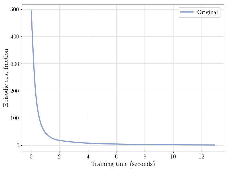
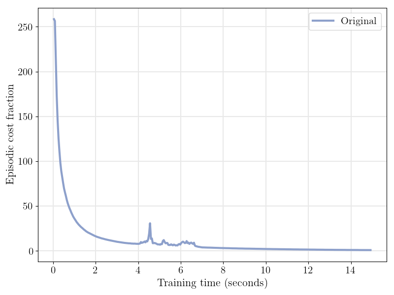
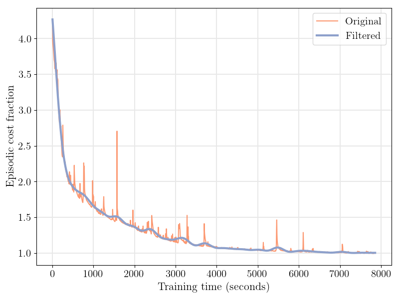
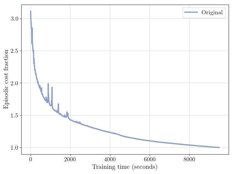
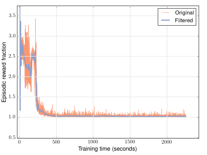
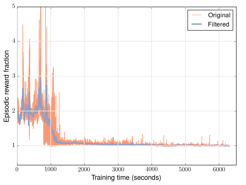
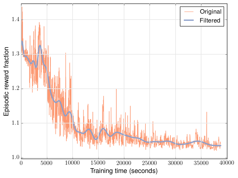
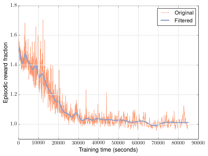
D2C implementation is done in three stages corresponding to those mentioned in the previous section and ‘MuJoCo Pro 150’ is used as the environment for simulating the blackbox model. An off-the-shelf implementation of DDPG provided by Keras-RL [27] library has been customized for our simulations. It may be noted that the structure of the reward function is formulated to optimize the performance of DDPG and hence, different from that used in D2C. However, the episode length (or horizon) and the time-discretization step is held identical. Although continuous RL algorithms such as DDPG learn the policy and thereby interpolating it to the entire state space, we consider the task-based experiments in a finite limited time-frame window approach. Training is performed until the neural networks’ loss is converged. Hence, though the episodic reward does seem to converge earlier, that itself may not indicate that the policy is converged.

For fair comparison, ‘Episodic reward/cost fraction’ is considered with both methods. It is defined as the fraction of reward obtained in an episode during training w.r.t the nominal episodic reward (converged reward). Note that the words ’reward’ and ’cost’ are being used interchangeably due to their different notions in optimal control and RL literature respectively, though they achieve the same objective. For simplicity, one is considered the negative of the other.

V-B Performance Comparison

Data-efficiency: As mentioned above, an efficient training is one that requires minimal data sampling in order to achieve the same behavior. One way of measuring it is to collate the times taken for the episodic cost (or reward) to converge during training. Plots in Fig. 1 show the training process with both methods on the systems considered. Table I delineates the times taken for training respectively. As the system identification and feedback gain calculation in case of D2C take only a small portion of time, the total time comparison in (Table I) shows that D2C learns the optimal policy substantially faster than DDPG and hence, has a better data efficiency.

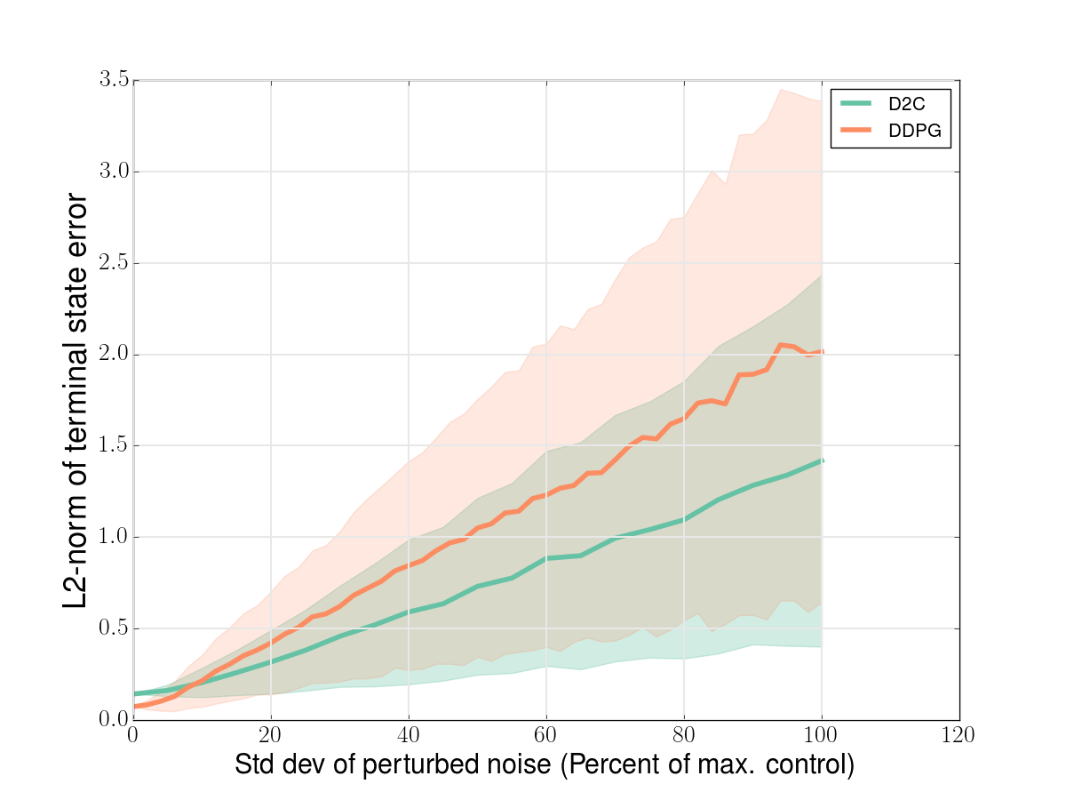
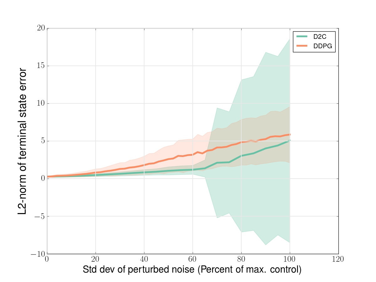
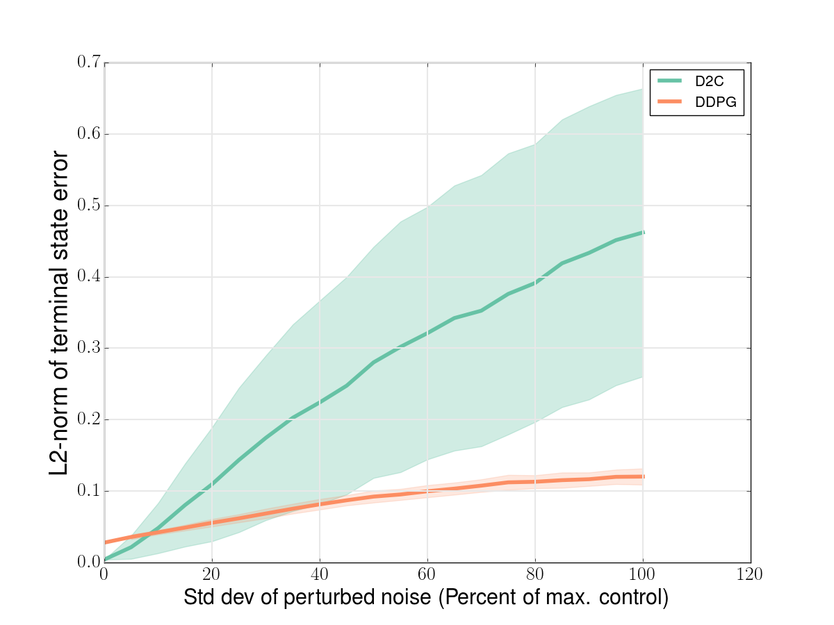
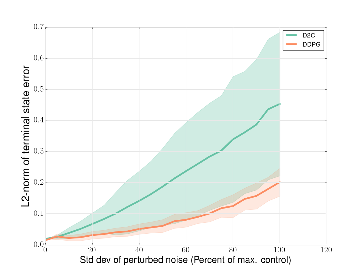
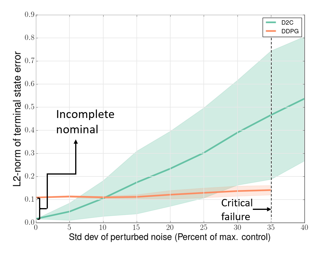
Robustness to noise: As with canonical off-policy RL algorithms, DDPG requires that an exploration noise be added to the policy, during training. Given that the training adapts the policy to various levels of noise, combined with hours of intense training and a nonlinear policy output, it is expected that it is more robust towards noise as is evident from Figs. 2 (c) and 2 (d). However, from plots in Figs. 2 (a) and (b), it is evident that in some systems the performance of D2C is on par with or better than DDPG. It may also be noted that the error variance in D2C method increases abruptly when the noise level is higher than a threshold and drives the system too far away from the nominal trajectory that the LQR controller cannot fix it. This could be considered as a drawback for D2C. However, it must be noted that the range of noise levels (up until 100 % of the maximum control signal) that we are considering here is far beyond what is typically encountered in practical scenarios. Hence, even in swimmer examples, the performance of D2C is tolerable to a reasonable extent of noise in the system.

Ease of training: The ease of training is often an ignored topic in analyzing a reinforcement learning (RL) algorithm. By this, we mean the challenges associated with its implementation. As with many RL algorithms that involve neural networks, DDPG has no guarantees for policy convergence. As a result, the implementation often involves tuning a number of hyper-parameters and a careful reward shaping in a trial and error fashion, which is even more time-consuming given that their successful implementation already involves significant time and computational resources. Reproducibility [11] is still a major challenge that RL is yet to overcome. On the other hand, training in our approach is predictable and very reliable.

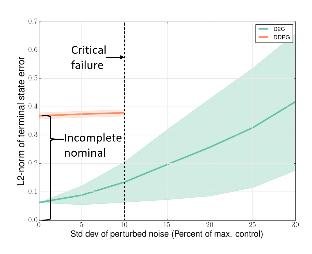
To elucidate the ease of training from an empirical perspective, the exploration noise that is required for training in DDPG mandates the system to operate with a shorter time-step than a threshold, beyond which the simulation fails due to an unbearable magnitude of control actions into the system. For this, we train both the swimmers in one such case (with $\Delta t=0.01$ sec) till it fails and execute the intermediate policy. Fig. 3 shows the plot in the testing-stage with both methods. It is evident from the terminal state mean-squared error at zero noise level that the nominal trajectory of DDPG is incomplete and its policy failed to reach the goal. The effect is more pronounced in the higher-dimensional 6-link swimmer system (Fig. 3b), where the DDPG’s policy can be deemed to be downright broken. Note, from Table I, that the systems have been trained with DDPG for a time that is more than thrice with the 3-link swimmer and 4 times with the 6-link swimmer. On the other hand, under same conditions, the seamless training of D2C results in a working policy with even greater data-efficiency.

TABLE I: Simulation parameters and training outcomes

System	Steps per	Time-	Training time (in sec.)
	episode	step	D2C
		(in sec.)	Open-	Closed-	DDPG
			loop	loop
Inverted	30	0.1	12.9	$<0.1$	2261.15
Pendulum
Cart pole	30	0.1	15.0	1.33	6306.7
3-link	1600	0.005	7861.0	13.1	38833.64
Swimmer	800	0.01	4001.0	4.6	13280.7*
6-link	1500	0.006	9489.3	26.5	88160
Swimmer	900	0.01	3585.4	16.4	15797.2*

(a) 3-link swimmer

(b) 6-link swimmer

Figure 3: D2C vs DDPG at $\Delta t=0.01s$

VI CONCLUSIONS

In this paper, we proposed a near-optimal control algorithm under fully observed conditions and showed that our method is able to scale-up to higher dimensional state-space without any knowledge about the system model. Due to sequential calculation used in the open-loop optimization and the system identification, D2C is highly memory efficient and also convenient for parallelization. We tested its performance and juxtaposed them with a state-of-the-art deep RL technique - DDPG. From the results, our method has conspicuous advantages over DDPG in terms of data efficiency and ease of training. The robustness of D2C is also better in some cases, but has scope for further development by employing more sophisticated feedback methods and ensuring that the data efficiency is not compromised. We also believe further drastic reduction in the planning time can be achieved by parallelization and a more sophisticated parametrization of the open loop problem.

It is evident from the simulations that methods such as D2C are able to achieve their goals accurately whereas DDPG consumes inordinate amount of time in ‘fine-tuning’ their behavior towards the goal. However, we also note that, by doing this, DDPG is tentatively exploring over the entire state-space and can result in a better generic policy. Another drawback with D2C over canonical RL algorithms is that the cost could be stuck in a local minimum, whereas DDPG due to the nature of stochastic gradient descent in training neural networks, can potentially reach the globally optimal solution. Nevertheless, we hope that our approach signifies the potential of decoupling based approaches such as D2C in a reinforcement learning paradigm and recognizes the need for more hybrid approaches that complement the merits of each.

APPENDIX

VI-A Proof of Lemma 1

Proof:

We proceed by induction. The first general instance of the recursion occurs at $t=3$. It can be shown that:

$$\delta x_{3}=\underbrace{(\bar{A}_{2}\bar{A}_{1}(\epsilon w_{0})+\bar{A}_{2}(\epsilon w_{1})+\epsilon w_{2})}_{\delta x_{3}^{l}}+$$

$$\underbrace{\{\bar{A}_{2}\bar{S}_{1}(\epsilon w_{0})+\bar{S}_{2}(\bar{A}_{1}(\epsilon w_{0})+\bar{S}_{2}(\bar{A}_{1}(\epsilon w_{0})+\epsilon w_{1}+\bar{S}_{1}(\epsilon w_{0}))\}}_{\bar{\bar{S}}_{3}}.$$ (30)

Noting that $\bar{S}_{1}(.)$ and $\bar{S}_{2}(.)$ are second and higher order terms, it follows that $\bar{\bar{S}}_{3}$ is $O(\epsilon^{2})$.
Suppose now that $\delta x_{t}=\delta x_{t}^{l}+\bar{\bar{S}}_{t}$ where $\bar{\bar{S}}_{t}$ is $O(\epsilon^{2})$. Then:

$$\delta x_{t+1}=\bar{A}_{t+1}(\delta x_{t}^{l}+\bar{\bar{S_{t}}})+\epsilon w_{t}+\bar{S}_{t+1}(\delta x_{t}),$$

$$=\underbrace{(\bar{A}_{t+1}\delta x_{t}^{l}+\epsilon w_{t})}_{\delta x_{t+1}^{l}}+\underbrace{\{\bar{A}_{t+1}\bar{\bar{S}}_{t}+\bar{S}_{t+1}(\delta x_{t})\}}_{\bar{\bar{S}}_{t+1}}.$$ (31)

Noting that $\bar{S}_{t+1}$ is $O(\epsilon^{2})$ and that $\bar{\bar{S}}_{t+1}$ is $O(\epsilon^{2})$ by assumption, the result follows. ∎

VI-B Lemma 2

Lemma 2

Let $\delta J_{1}^{\pi}$, $\delta J_{2}^{\pi}$ be as defined in (13). Then, $\mathbb{E}[\delta J_{1}\delta J_{2}]$ is an $O(\epsilon^{4})$ function.

Proof:

In the following, we suppress the explicit dependence on $\pi$ for $\delta J_{1}^{\pi}$ and $\delta J_{2}^{\pi}$ for notational convenience. Recall that $\delta J_{1}=\sum_{t=0}^{T}c_{t}^{x}\delta x_{t}^{l}$, and $\delta J_{2}=\sum_{t=0}^{T}\bar{H}_{t}(\delta x_{t})+c_{t}^{x}\bar{\bar{S}}_{t}$. For notational convenience, let us consider the scalar case, the vector case follows readily at the expense of more elaborate notation. Let us first consider $\bar{\bar{S}}_{2}$. We have that $\bar{\bar{S}}_{2}=\bar{A}_{2}\bar{S}_{1}(\epsilon w_{0})+\bar{S}_{2}(\bar{A}_{1}(\epsilon w_{0})+\epsilon w_{1}+\bar{S}_{1}(\epsilon w_{0}))$. Then, it follows that:

$$\bar{\bar{S}}_{2}=\bar{A}_{2}\bar{S}_{1}^{(2)}(\epsilon w_{0})^{2}+\bar{S}_{2}^{(2)}(\bar{A}_{1}\epsilon w_{0}+\epsilon w_{1})^{2}+O(\epsilon^{3}),$$ (32)

where $\bar{S}_{t}^{(2)}$ represents the coefficient of the second order term in the expansion of $\bar{S}_{t}$. A similar observation holds for $H_{2}(\delta x_{2})$ in that:

$$\bar{H}_{2}(\delta x_{2})=\bar{H}_{2}^{(2)}(\bar{A}_{1}(\epsilon w_{0})+\epsilon w_{1})^{2}+O(\epsilon^{3}),$$ (33)

where $\bar{H}_{t}^{(2)}$ is the coefficient of the second order term in the expansion of $\bar{H}_{t}$. Note that $\epsilon w_{0}=\delta x_{1}^{l}$ and $\bar{A}_{1}(\epsilon w_{0})+\epsilon w_{1}=\delta x_{2}^{l}$. Therefore, it follows that we may write:

$$\bar{H}_{t}(\delta x_{t})+C_{t}^{x}\bar{\bar{S}}_{t}=\sum_{\tau=0}^{t-1}q_{t,\tau}(\delta x_{\tau}^{l})^{2}+O(\epsilon^{3}),$$ (34)

for suitably defined coefficients $q_{t,\tau}$. Therefore, it follows that

$$\delta J_{2}=\sum_{t=1}^{T}\bar{H}_{t}(\delta x_{t})+C_{t}^{x}\bar{\bar{S}}_{t}$$

$$=\sum_{\tau=0}^{T}\bar{q}_{T,\tau}(\delta x_{\tau}^{l})^{2}+O(\epsilon^{3}),$$ (35)

for suitably defined $\bar{q}_{T,\tau}$. Therefore:

$$\delta J_{1}\delta J_{2}=\sum_{t,\tau}C_{\tau}^{x}(\delta x_{\tau}^{l})\bar{q}_{T,t}(\delta x_{t}^{l})^{2}+O(\epsilon^{4}).$$ (36)

Taking expectations on both sides:

$$E[\delta J_{1}\delta J_{2}]=\sum_{t,\tau}C_{\tau}^{x}\bar{q}_{T,t}E[\delta x_{\tau}^{l}(\delta x_{t}^{l})^{2}]+O(\epsilon^{4}).$$ (37)

Break $\delta x_{t}^{l}=(\delta x_{t}^{l}-\delta x_{\tau}^{l})+\delta x_{\tau}^{l}$, assuming $\tau<t$. Then, it follows that:

$$E[\delta x_{\tau}^{l}(\delta x_{t}^{l})^{2}]=E[\delta x_{\tau}^{l}(\delta x_{t}^{l}-\delta x_{\tau}^{l})^{2}]+E[(\delta x_{\tau}^{l})^{3}]$$

$$+2E[(\delta x_{t}^{l}-\delta x_{\tau}^{l})(\delta x_{\tau}^{l})^{2}]$$

$$=E[(\delta x_{\tau}^{l})^{3}],$$ (38)

where the first and last terms in the first equality drop out due to the independence of the increment $(\delta x_{t}^{l}-\delta x_{\tau}^{l})$ from $\delta x_{\tau}^{l}$, and the fact that $E[\delta x_{t}^{l}-\delta x_{\tau}^{l}]=0$ and $E[\delta x_{\tau}^{l}]=0$. Since $\delta x_{\tau}^{l}$ is the state of the linear system $\delta x_{t+1}=\bar{A}_{t}\delta x_{t}^{l}+\epsilon w_{t}$, it may again be shown that:

$$E[\delta x_{\tau}^{l}]^{3}=\sum_{s_{1},s_{2},s_{3}}\Phi_{\tau,s_{1}}\Phi_{\tau,s_{2}}\Phi_{\tau,s_{3}}E[w_{s_{1}}w_{s_{2}}w_{s_{3}}],$$ (39)

where $\Phi_{t,\tau}$ represents the state transitions operator between times $\tau$ and $t$, and follows from the closed loop dynamics. Now, due to the independence of the noise terms $w_{t}$, it follows that $E[w_{s_{1}}w_{s_{2}}w_{s_{3}}]=0$ regardless of $s_{1},s_{2},s_{3}$.
An analogous argument as above can be repeated for the case when $\tau>t$. Therefore, it follows that $E[\delta J_{1}\delta J_{2}]=O(\epsilon^{4})$. ∎

References

- [1] P. R. Kumar and P. Varaiya, Stochastic systems: Estimation, identification, and adaptive control. SIAM, 2015, vol. 75.
- [2] P. A. Ioannou and J. Sun, Robust adaptive control. Courier Corporation, 2012.
- [3] K. J. Åström and B. Wittenmark, Adaptive control. Courier Corporation, 2013.
- [4] S. Sastry and M. Bodson, Adaptive control: stability, convergence and robustness. Courier Corporation, 2011.
- [5] D. Silver, A. Huang, C. J. Maddison, A. Guez, L. Sifre, G. Van Den Driessche, J. Schrittwieser, I. Antonoglou, V. Panneershelvam, M. Lanctot et al., “Mastering the game of go with deep neural networks and tree search,” nature, vol. 529, no. 7587, p. 484, 2016.
- [6] T. P. Lillicrap, J. J. Hunt, A. Pritzel, N. Heess, T. Erez, Y. Tassa, D. Silver, and D. Wierstra, “Continuous control with deep reinforcement learning,” arXiv preprint arXiv:1509.02971, 2015.
- [7] S. Levine, C. Finn, T. Darrell, and P. Abbeel, “End-to-end training of deep visuomotor policies,” The Journal of Machine Learning Research, vol. 17, no. 1, pp. 1334–1373, 2016.
- [8] W. Yuhuai, M. Elman, L. Shun, G. Roger, and B. Jimmy, “Scalable trust-region method for deep reinforcement learning using kronecker-factored approximation,” arXiv:1708.05144, 2017.
- [9] S. John, L. Sergey, M. Philipp, J. Michael I., and A. Pieter, “Trust region policy optimization,” arXiv:1502.05477, 2017.
- [10] S. John, W. Filip, D. Prafulla, R. Alec, and K. Oleg, “Proximal policy optimization algorithms,” arXiv:1707.06347, 2017.
- [11] P. Henderson, R. Islam, P. Bachman, J. Pineau, D. Precup, and D. Meger, “Deep reinforcement learning that matters,” in Thirty-Second AAAI Conference on Artificial Intelligence, 2018.
- [12] S. Gu, T. Lillicrap, Z. Ghahramani, R. E. Turner, and S. Levine, “Q-prop: Sample-efficient policy gradient with an off-policy critic,” arXiv preprint arXiv:1611.02247, 2016.
- [13] M. Falcone, “Recent Results in the Approximation of Nonlinear Optimal Control Problems,” in Large-Scale Scientific Computing LSSC, 2013.
- [14] D. Jacobsen and D. Mayne, Differential Dynamic Programming. Elsevier, 1970.
- [15] E. Theoddorou, Y. Tassa, and E. Todorov, “Stochastic Differential Dynamic Programming,” in Proceedings of American Control Conference, 2010.
- [16] E. Todorov and W. Li, “A generalized iterative LQG method for locally-optimal feedback control of constrained nonlinear stochastic systems,” in Proceedings of American Control Conference, 2005, pp. 300 – 306.
- [17] W. Li and E. Todorov, “Iterative linearization methods for approximately optimal control and estimation of non-linear stochastic system,” International Journal of Control, vol. 80, no. 9, pp. 1439–1453, 2007.
- [18] W. B. Powell, Approximate Dynamic Programming: Solving the curses of dimensionality. John Wiley & Sons, 2007.
- [19] D. Bertsekas, Dynamic programming and optimal control. Athena scientific Belmont, MA, 2012, vol. 2.
- [20] R. S. Sutton and A. G. Barto, Reinforcement learning: An introduction. MIT press, 2018.
- [21] D. Yu, M. Rafieisakhaei, and S. Chakravorty, “Stochastic Feedback Control of Systems with Unknown Nonlinear Dynamics,” in 56th IEEE Conference on Decision and Control(CDC), 2017.
- [22] M. Rafieisakhaei, S. Chakravorty, and P. R. Kumar, “A Near-Optimal Separation Principle for Nonlinear Stochastic Systems Arising in Robotic Path Planning and Control,” in 56th IEEE Conference on Decision and Control(CDC), 2017.
- [23] R. Wang, K. Parunandi, D. Yu, D. Kalathil, and S. Chakravorty, “Decoupled data based approach for learning to control nonlinear dynamical systems,” Tech. Report. Available at https://goo.gl/pd3pRU, March, 2019.
- [24] T. Lillicrap et al., “Continuous control with deep reinforcement learning,” in Proc. ICLR, 2016.
- [25] T. Emanuel, E. Tom, and Y. Tassa, “Mujoco: A physics engine for model-based control,” IEEE/RSJ International Conference on Intelligent Robots and Systems, pp. 5026–5033, 2012.
- [26] T. Yuval and et al., “Deepmind control suite,” arXiv:1801.00690, 2018.
- [27] M. Plappert, “keras-rl,” https://github.com/keras-rl/keras-rl, 2016.