The 3XMM/SDSS Stripe 82 Galaxy Cluster Survey
II. X-ray and optical properties of the cluster sample

Abstract

We present X-ray and optical properties of the optically confirmed galaxy cluster sample from the 3XMM/SDSS Stripe 82 cluster survey. The sample includes 54 galaxy clusters in the redshift range of 0.05-1.2, with a median redshift of 0.36. We first present the X-ray temperature and luminosity measurements that are used to investigate the X-ray luminosity-temperature relation. The slope and intercept of the relation are consistent with those published in the literature. Then, we investigate the optical properties of the cluster galaxies including their morphological analysis and the galaxy luminosity functions. The morphological content of cluster galaxies is investigated as a function of cluster mass and distance from the cluster center. No strong variation of the fraction of early and late type galaxies with cluster mass is observed. The fraction of early type galaxies as a function of cluster radius varies as expected. The individual galaxy luminosity functions (GLFs) of red sequence galaxies were studied in the five ugriz bands for 48 clusters. The GLFs were then stacked in three mass bins and two redshift bins. Twenty clusters of the present sample are studied for the first time in X-rays, and all are studied for the first time in the optical range. Altogether, our sample appears to have X-ray and optical properties typical of “average” cluster properties.

1 Introduction

Galaxy clusters are the largest massive structures in the universe which contain hundreds to thousands of galaxies within spatial regions of a few Mpc. They also contain gas in their intracluster medium (ICM) that is smoothly distributed and filling the intergalactic space. The hot ICM is a key feature in studying galaxy clusters since it is a strong X-ray emitter, which allows the identification process up to high redshifts and reveals that clusters are well defined and connected structural entities. The study of galaxy clusters gives the opportunity to investigate the physical processes behind the formation and evolution of their baryonic components (galaxies and gas) and to probe the distribution of matter in the universe (e.g. Böhringer, 2008; Allen et al., 2011).

The X-ray selection of galaxy clusters has several advantages for cosmological studies: the observable X-ray temperature and luminosity of a cluster is tightly correlated with the cluster total mass, which is the most fundamental parameter for clusters (Reiprich & Böhringer, 2002). Also, the cluster X-ray luminosity correlates well with its temperature (${\rm L_{X}-T_{X}}$), following the relation predicted by cluster formation models. For example, the self-similar model (Kaiser, 1986) simply predicts that clusters formed by gravitational collapse in the universe and that massive galaxy clusters are a scaled version of small clusters. Hence, cluster masses can be inferred from scaling relations found between cluster observable properties. Many studies stated that the slope of the ${\rm L_{X}-T_{X}}$ relation is steeper than that expected from a self-similar model (${\rm L_{X}\propto T_{X}^{2}}$) for various samples of galaxy groups and clusters (e.g. Pratt et al., 2009; Hilton et al., 2012; Takey et al., 2013; Giles et al., 2016). It is also important to track the ${\rm L_{X}-T_{X}}$ relation with redshift since different heating mechanisms can be involved.

Galaxy clusters are also considered as the largest astrophysical laboratories that are suitable to investigate the galaxy formation, evolution, and morphological properties within a well defined dense environment. This environment is known to influence galaxy properties. Morphological segregation of galaxies in clusters was indeed found to be strong since the seminal paper of Dressler (1980), who showed for a sample of 55 nearby clusters ($z<0.07$) that early-type galaxies were dominant in the central regions of clusters while late-type galaxies were more abundant in the outskirts. It was later shown to be also the case in more distant clusters and explained by the fact that numerous galaxy mergers take place in cluster centers, thus creating a large population of early-type galaxies, while late-type galaxies are continuously accreted from the field onto clusters along the cosmic filaments at the intersection of which clusters are believed to be located (e.g. Adami et al., 2009). Galaxy luminosity functions (GLFs) have also been found to depend on the environment, with a difference between cluster and field galaxies, and a flattening of the GLF as the environment becomes less dense (as described in detail in Martinet et al. (2015) and references therein).

In a previous paper on galaxy clusters in the SDSS Stripe 82, Durret et al. (2015) investigated the fraction of late-type to early-type galaxies with cluster redshift. They also investigated the evolution of the galaxy luminosity function with redshift. This study was based on cluster candidates with only photometric redshifts extracted from the SDSS Stripe 82 (S82, hereafter) data.

In the present paper, we investigate the above mentioned studies (${\rm L_{X}-T_{X}}$ relation, morphological analysis, and galaxy luminosity function) for the galaxy cluster sample conducted in the cluster survey published by Takey et al. (2016). The cluster sample includes X-ray selected and optically confirmed clusters from XMM-Newton and S82 data, respectively. We will first investigate the relation between the X-ray luminosity and temperature of the cluster sample, which spans a wide redshift range. We will then study the morphology and luminosity function of cluster galaxies in our sample as a function of cluster properties (cluster mass and redshift).

The paper structure is as follows. We first present in Sect. 2 the cluster sample used in our analysis. X-ray data reduction and analysis as well as the ${\rm L_{X}-T_{X}}$ relation are presented in Sect. 3. The morphological properties and galaxy luminosity functions of cluster galaxies are presented in Sects. 4 and 5, respectively. We finally summarise our work and conclude in Sect. 6. We use the cosmological constants $\Omega_{\rm M}=0.3$, $\Omega_{\Lambda}=0.7$ and $H_{0}=70$ km s^-1 Mpc^-1 throughout the paper.

2 The galaxy cluster sample

We have published a galaxy group/cluster catalogue in the framework of the 3XMM/SDSS Stripe 82 galaxy cluster survey (Takey et al., 2016). The survey was based on X-ray extended sources from the third XMM-Newton serendipitous source catalogue (3XMM-DR5, Rosen et al., 2016) that are located on the sky coverage of the SDSS S82. The survey area is 11.25 deg² due to the relatively small number of XMM-Newton observations (74 pointings) targeting celestial objects and/or positions in the S82 footprint. We limited the cluster search to sources located in the S82 region, where the optical data are deeper than in the normal SDSS survey. These 74 observations span a wide range of exposure times (good time intervals) from 2 ks to 65 ks. Also, these observations are clean ones that have only a masked area $\leq 1\%$. The masked areas are not suitable for source detections. We also required that at least one of the EPIC cameras is used in full frame mode, so that the full field of view is exposed.

We then selected all the X-ray extended sources from the 3XMM-DR5 catalogue that are detected in the EPIC images of the 74 observations considered in our cluster survey. This list includes 120 detections that contain multiple and spurious detections. By avoiding the multiplicity and removing possible spurious detections through visual inspection of their X-ray and optical images, the X-ray galaxy cluster candidate list comprises 94 extended sources. By cross-matching this list with six X-ray and optically selected cluster catalogues and by searching the NASA/IPAC Extragalactic Database (NED), we constructed a cluster catalogue comprising 54 galaxy clusters that are known in the literature with measured redshifts. The remaining candidates (40 sources) have no redshifts in the literature and are expected to be distant clusters. The list of the galaxy cluster catalogue (54 clusters) and the 40 X-ray cluster candidates are published in our first paper by Takey et al. (2016).

The present study is based on our published cluster catalogue that comprises 54 galaxy groups/clusters in the redshift range from 0.05 to 1.2 with a median redshift of 0.36.The redshifts of these clusters were obtained from cross-correlated X-ray and optical cluster catalogues or from the NED. We confirm published redshift values, based on photometric and spectroscopic data available in the SDSS. A spectroscopic confirmation based on at least one member galaxy with spectroscopic redshift is available for 51 clusters of our sample. Fig. 1 shows the cluster redshift distribution for the 51 clusters with spectroscopic redshifts and for the subsample of 37 clusters with X-ray data of sufficient quality to allow the determination of the X-ray temperatures and luminosities that are used to investigate the ${\rm L_{X}-T_{X}}$ relation (see Sect. 3.2).

About two thirds of the cluster sample were known in previous X-ray selected cluster catalogues (e.g. Mehrtens et al., 2012; Takey et al., 2013, 2014) while the remaining systems are newly discovered in X-rays. The X-ray luminosities and masses of the clusters were estimated based on the fluxes given in the 3XMM-DR5 catalogue. The galaxy cluster catalogue is availble at the CDS.

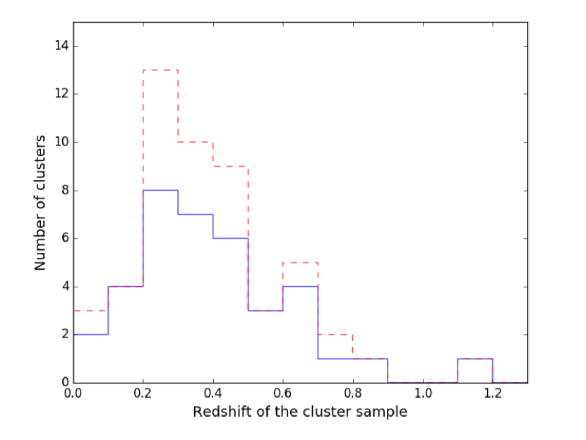
Figure 1: Redshift distributions. Red dashed: full sample of 51 clusters with spectroscopic redshifts, blue solid: subsample of 37 clusters considered to investigate the ${\rm L_{X}-T_{X}}$ relation

3 X-ray properties of the cluster sample

We present here our procedure to reduce and analyse the XMM-Newton observations of the cluster sample. Since the X-ray data quality is not sufficient to determine the X-ray temperature profiles of the systems, we compute the global temperatures and luminosities in a radius of 300 kpc. We expect to derive X-ray temperatures and luminosities with reasonable uncertainties for about two thirds of the cluster sample that have more than 300 photon counts. These measurements will be used to investigate the X-ray luminosity-temperature (${\rm L_{X}-T_{X}}$) relation, as described below.

3.1 X-ray data reduction and analysis

The 54 galaxy clusters constituting our sample were detected in 31 XMM-Newton observations. A few clusters are detected in more than one XMM pointing. In this case, we choose the observation with the higher photon counts to extract the X-ray spectrum. The observation data files (ODFs, raw data) were downloaded using the Archive InterOperability System (AIO), which provides access to the XMM-Newton Science Archive (XSA). Both the data reduction and analysis of the sample were carried out using the XMM-Newton Science Analysis Software (SAS: Arviset et al., 2002) version 15.0.0, following the recommended standard pipelines in the SAS manuals. To reduce the ODFs, we first generated the calibrated event list for the EPIC (MOS1, MOS2, PN) cameras using the latest calibration data. This step was done with the SAS tasks $\tt{cifbuild,odfingest,epchain,emchain}$.

We then filtered the calibrated event lists by excluding observing intervals with high background flares and bad events. To do this, we followed the procedure recommended in the user guide of SAS, which has the following steps; (i) We first created a light curve of the event file to check for bad pixels and columns, and high-background periods. (ii) We then created a Good Time Interval (GTI) file that contains the good times corresponding to a background count rate that is approximately constant and low. This GTI file is used to filter the event list. (iii) We applied the standard filter expression and the GTI to create a filtered event list. (iv) Finally, we created a second light curve of the filtered event list to check the removal of high-background periods. The filtered calibrated event lists were used to create sky images in different energy bands. These last steps were done with the SAS packages $\tt{evselect,tabgtigen,xmmselect}$.

The X-ray spectra of clusters were extracted from the EPIC filtered calibrated event lists within fixed circular apertures of radius 300 kpc centered on the X-ray emission peaks. This fixed source aperture was chosen because the spectral analysis could not be achieved with reasonable accuracy within $R_{500}$ for most of the cluster sample due to their X-ray data quality. $R_{500}$ is the radius at which the cluster average density equals 500 times the critical density of the Universe estimated at the cluster redshift.

A background spectrum for each cluster is also extracted in a fixed annulus with inner and outer radii equaling three (900 kpc) and four (1200 kpc) times the source extraction radius (300 kpc), respectively. Other sources overlapping the cluster circular and background annulus apertures are excluded from the regions used to extract spectra. The SAS meta task $\tt{especget}$ is used to generate the cluster and background spectra and to create the response matrix files (redistribution matrix file (RMF) and ancillary response file (ARF)) that are required to perform the X-ray spectral fitting.

Before any fit, the photon counts of the cluster spectra are grouped into bins with at least one count per bin (as e.g. in Takey et al., 2013; Ogrean et al., 2016) using the Ftools task $\tt{grppha}$. For spectral fitting, we use the XSPEC version 12.9.0n (Arnaud, 1996) run by Python module $\tt{Pyspec}$.

The EPIC spectra of each cluster are simultaneously fit by a combination of the $\tt{TBABS}$ absorption model (Wilms et al., 2000) and of a single-temperature optically thin thermal plasma $\tt{APEC}$ model (Smith et al., 2001). In the fitting process, we fix the Galactic hydrogen density column (nH) to the value derived from the Leiden/Argentine/Bonn (LAB) survey (Kalberla et al., 2005). We also fix both the cluster redshift to the value given in the cluster catalogue and the metallicity to 0.3 $Z_{\odot}$. We used the spectroscopic redshifts for 51 systems and the photometric redshifts for the remaining three clusters.

The free parameters of the $\tt{APEC}$ model are the X-ray temperature and the spectral normalization. We use the Cash statistics in the fitting process and the energy range is [0.3-7] keV. We limited the energy range to 0.3-7 keV because the XMM telescope is poorly calibrated at energies softer than 0.3 keV and the cluster spectra are background dominated at energies higher than 7 keV (Lloyd-Davies et al., 2011). The results are the cluster X-ray temperature, aperture flux and luminosity (rest frame) in the [0.5-2] keV band, and their corresponding errors. The errors on the fit parameters are given in the 68 percent confidence range. We also derive the bolometric X-ray flux and luminosity (rest frame) in [0.1-50] keV from the dummy response matrices based on the best fit parameters. The bolometric flux and luminosity are derived with no errors. Here, we assume that the relative error on the bolometric luminosity is the same as that on the luminosity in the [0.5-2] keV band produced by the fit, and the errors on the bolometric flux and luminosity are estimated in this way. To make sure this assumption is valid and the resulting luminosity does not depend too much on temperature errors, we varied the temperatures by $\pm 1\sigma$ in a few cases and found that the measured band luminosities are within their errors.

3.2 The X-ray luminosity-temperature (${\rm L_{X}-T_{X}}$) relation

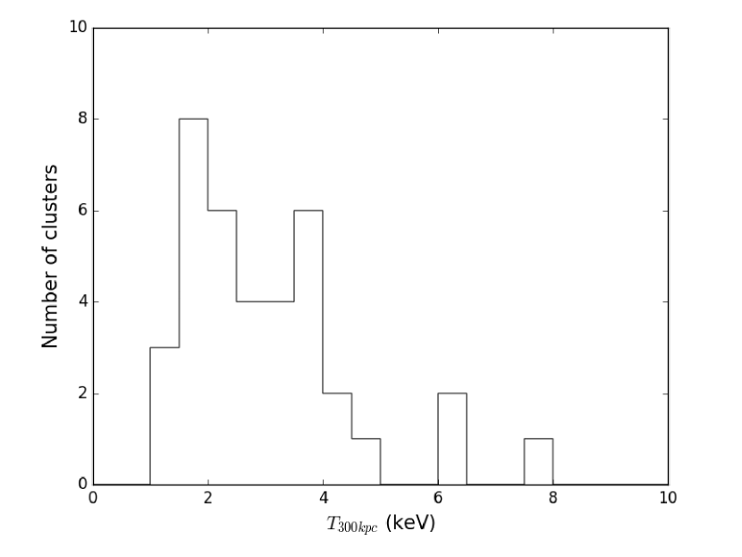
Figure 2: Distribution of X-ray temperatures for 37 clusters used in ${\rm L_{X}-T_{X}}$ relation

In the ${\rm L_{X}-T_{X}}$ relation, we only include the 37 galaxy clusters (69%) from the cluster sample that have relative errors on temperatures and luminosities smaller than 50%. This was done to obtain a relation with a slope and an intrinsic scatter unaffected by large uncertainties on temperatures and luminosities. The properties of the 37 clusters considered to compute the ${\rm L_{X}-T_{X}}$ relation are given in the Appendix (Table A1). The median, mean, and standard deviation of the temperature relative errors are 22%, 21%, and 11%, respectively. The majority of the clusters in this subsample have low temperatures, below 4 keV. Fig. 2 shows the distribution of X-ray temperatures of the studied sample.

The redshift range of the cluster sample (37 systems) is from 0.07 to 1.2, with a median redshift of 0.36. There are 10 distant clusters in the cluster sample with redshifts beyond 0.5. Figure 1 shows the cluster redshift distribution for the systems used in the ${\rm L_{X}-T_{X}}$ relation.

To check our results on cluster temperatures, we compare the temperatures derived within 300 kpc with those published within a different aperture (that maximize the signal-to-noise ratio) in the 2XMMi/SDSS catalogue by Takey et al. (2013). Figure 3 shows a good agreement with no systematics for the 13 clusters in common between our cluster sample and the 2XMMi/SDSS cluster sample.

The advantage of having derived temperatures within an aperture of 300 kpc, is that it allows a direct comparison of our ${\rm L_{X}-T_{X}}$ relation with that published by Giles et al. (2016), who also determined the temperature within 300 kpc and the luminosity within $R_{500}$ for a sample of clusters of comparable redshifts. Giles et al. (2016) investigated the ${\rm L_{X}-T_{X}}$ relation for the 100 brightest galaxy clusters detected in the XXL survey made by the XMM-Newton mission. Also, the temperatures within 300 kpc are comparable to the temperatures within apertures that represent the highest signal-to-noise ratio published by Takey et al. (2013), see Fig. 3.

The X-ray temperature measurements within $R_{500}$ and 300 kpc are comparable, with no systematic differences, as shown by Giles et al. (2016). To check if this agreement is valid in our cluster sample, we extracted spectra within $R_{500}$ for 15 systems with fluxes in [0.5-2] keV band higher than $5\times 10^{-14}$ erg cm^-2 s^-1. The fluxes and $R_{500}$ values are obtained from the catalogue published by Takey et al. (2016). We then fitted the spectra with the same procedure as used in the current analysis. The ratio of the temperatures within $R_{300~{}kpc}$ and $R_{500}$ has a mean and standard deviation of 1.035 and 0.258, respectively. This means that the temperatures within $R_{300~{}kpc}$ are comparable to those within $R_{500}$, since their mean increases by only 4%, which is much smaller than the mean relative error on the temperature (20%) for these 15 systems.

Figure 3: Comparison of X-ray temperatures measured in our study at a radius of 300 kpc and in the 2XMMi/SDSS survey at aperture that maximizes the signal-to-noise ratio. The plotted errors are the average of the positive and negative errors provided by the spectral analysis. The solid line shows the one-to-one relationship.

To investigate the ${\rm L_{X}-T_{X}}$ relation between the bolometric luminosity within $R_{500}$ ($L_{500}$ hereafter) and the temperature within 300 kpc, we first need to determine $L_{500}$ based on the aperture bolometric luminosity within 300 kpc ($L_{300~{}kpc}$ hereafter). We prefer to re-determine $L_{500}$ based on spectral fitting parameters from the present work, rather than taking $L_{500}$ from our earlier work (Takey et al., 2016), that was based on the fluxes from the 3XMM-DR5 catalogue.

The computing of $L_{500}$ is done through an iterative method to extrapolate the aperture (300 kpc) bolometric flux to the $R_{500}$ bolometric flux, $F_{500}$, by appplying the beta model, a hydrostatic isothermal model used to describe the X-ray surface brightness profiles $S(r)$ of galaxy clusters:

$$S(r)=S(0)\ \Bigg{[}1+\Big{(}\frac{r}{r_{\rm c}}\Big{)}^{2}\Bigg{]}^{-3\beta+1/2},$$ (1)

where r_c is the core radius. The model assumes that both the hot intracluster gas and the cluster galaxies are in hydrostatic equilibrium and isothermal.

To do this, we first computed the cluster mass within $R_{500}$, $M_{500}$, based on the $L_{500}-M_{500}$ relation from Pratt et al. (2009). The first input for this relation is the aperture bolometric luminosity, $L_{300~{}kpc}$. The output $M_{500}$ is used to compute a first estimate of $R_{500}$. The $L_{300~{}kpc}$ luminosity is also utilized to compute the cluster temperature at $R_{500}$, $T_{500}$, based on the $L_{500}-T_{500}$ relation from Pratt et al. (2009). The estimated value of $T_{500}$ is then considered to compute the cluster core radius and beta value based on published relations by Finoguenov et al. (2007). The beta model is then applied to calculate the fluxes enclosed within the aperture and within $R_{500}$. The ratio of the aperture to $R_{500}$ fluxes is utilized to extrapolate $L_{300~{}kpc}$ to the $R_{500}$ luminosity. This extrapolated luminosity is then considered as an input for another iteration and all computed parameters are updated. This iterative procedure is repeated until converging to a final solution, where the flux within the new estimated $R_{500}$ is the same as the previous flux in the iteration. At this stage, we computed the bolometric luminosity, $L_{500}$, that is used in investigating the ${\rm L_{X}-T_{X}}$ relation. The output luminosities, $L_{500}$, derived by this iterative method are comparable to the ones determined in the XMM Cluster Survey (XCS) by Mehrtens et al. (2012). The details of this method, the scaling relations, and the comparison of $L_{500}$ were described by Takey et al. (2011, 2013).

We fit the ${\rm L_{X}-T_{X}}$ relation for our cluster sample using the BCES orthogonal regression method (bces Python module, Akritas & Bershady, 1996) taking into account the errors on the luminosity and temperature as well as the intrinsic scatter of the relation. It is important to take into account the intrinsic scatter/dispersion of the ${\rm L_{X}-T_{X}}$ relation since the data points do not lie exactly on a straight line and this line is not of slope 1. The fit is applied to the 37 clusters with relative errors on the temperatures and luminosities smaller than 50%.

Figure 4 shows the ${\rm L_{X}-T_{X}}$ relation for our cluster sample. The best fit slope ($3.12\pm 0.56$) is in agreement with the value ($3.03\pm 0.28$) derived for the 100 brightest clusters in the XXL project published by Giles et al. (2016), but our slope has a larger uncertainty, possibly due to the X-ray data quality. In addition, the quality of the data did not allow us to exclude the cluster core when extracting the spectra. Pratt et al. (2009) showed that the scatter in the relation is reduced by more than a factor of two when excluding the cluster central regions. We also find good agreement with the ${\rm L_{X}-T_{X}}$ relation slopes in the literature (e.g. Pratt et al., 2009; Mittal et al., 2011; Hilton et al., 2012; Takey et al., 2013; Rabitz et al., 2017).

Table 1 shows the slopes and intercepts of the ${\rm L_{X}-T_{X}}$ relations evaluated for various cluster samples in different redshift ranges including our cluster sample. It can be noticed that the slope from the present work agrees within one sigma error with the published ones. Regarding the intercept of the ${\rm L_{X}-T_{X}}$ relation, we find that the current value ($44.25\pm 0.19$) is in agreement with those published by Pratt et al. (2009); Takey et al. (2013); Giles et al. (2016) within one sigma and within two sigmas with those by Mittal et al. (2011); Hilton et al. (2012).

It is also noticed from the ${\rm L_{X}-T_{X}}$ relation (Figure 4) that the data points are scattered around the fitted line. To determine the intrinsic scatter in the luminosity $\sigma_{\rm log}L_{500}$, we followed the procedure utilized by Pratt et al. (2009). In that method, the raw scatter is first determined using the error-weighted orthogonal distances to the regression line (see Equations (3) and (4) in Pratt et al., 2009). Then the intrinsic scatter of the luminosity is computed as the mean value of the quadratic differences between the raw scatters and the statistical errors of luminosity. The intrinsic scatter error is determined as the standard error of its value. This yields that the intrinsic scatter of the luminosity $\sigma_{\rm log}L_{500}$ in the current ${\rm L_{X}-T_{X}}$ relation is $0.54\pm 0.09$, which is higher than the value ($0.32\pm 0.06$) of the REXCESS sample (Pratt et al., 2009) and the one ($0.48\pm 0.03$) of the 2XMM/SDSS sample (Takey et al., 2013). In a similar way, we compute the intrinsic scatter of temperature $\sigma_{\rm log}T_{300~{}kpc}$ ($0.14\pm 0.02)$, which is also higher than the one ($0.07\pm 0.01$) for the HIFLUGCS sample derived by Mittal et al. (2011).

We also derived the slope and intercept of the ${\rm L_{X}-T_{X}}$ relation in clusters of low ($z<0.3$) and high ($z\geq 0.3$) redshift and found values similar to those for the whole sample, within the error bars. This agrees with the fact that the slopes and intercepts found in the literature for various redshift ranges are comparable (see Table 1).

As mentioned above, our cluster survey is based on 94 X-ray cluster candidates selected from the 3XMM-DR5 extended sources that are located in the SDSS S82 region. Since the 3XMM catalogue is based on XMM observations with a wide range of exposure times, it is not an easy task to assess the completeness of the list of extended sources in this catalogue or to assess the selection function. The catalogue may miss some extended sources with low photon counts or large core radii, or may include them with incorrect parameters. This implies that our X-ray cluster candidate list is not a complete one, and that it is not a flux-limited sample. The effect of the selection function on the ${\rm L_{X}-T_{X}}$ relation cannot therefore be estimated from the current sample. Thus, checking the evolution of the relation is not possible.

Also, only 54 systems have been optically confirmed with redshift estimates. Of these, 37 clusters have a sufficient data quality to investigate the ${\rm L_{X}-T_{X}}$ relation. Therefore, there are missing clusters with measured redshifts ($54-37=17$ systems) and missing candidates with no redshift estimate ($94-54=40$ candidates). The majority of the missing clusters and/or candidates in the relation are distant objects that may have no significant effect on the slope of the relation (Hilton et al., 2012). However, if the missing clusters and/or candidates include galaxy groups with low luminosities and temperatures, this can make the slope of the relation shallower (Takey et al., 2013).

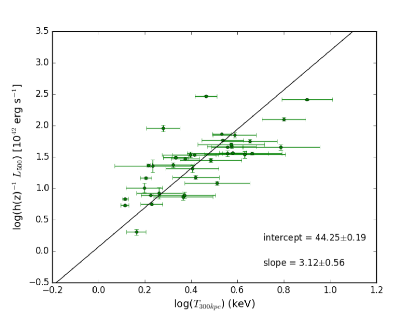
Figure 4: X-ray bolometric luminosity within $R_{500}$, $L_{500}$, plotted against X-ray temperature within 300 kpc for the 37 galaxy clusters that have relative errors on their luminosity and temperature smaller than 50%. The solid line represents the best fit to the data using a python module of the BCES orthogonal regression. The slope and intercept are written in the lower right corner.

Table 1: Comparison of the intercept and slope of the ${\rm L_{X}-T_{X}}$ relation with those published in the literature (N_ClGs is the number of clusters considered in the relation.)

Redshift	NClGs	Intercept	Slope	References
range
0.07 - 1.20	37	$44.25\pm 0.19$	$3.12\pm 0.56$	1
0.04 - 1.05	100	$44.10\pm 0.03$	$3.03\pm 0.28$	2
0.06 - 0.25	96	$44.63\pm 0.10$	$3.18\pm 0.22$	3
0.004 - 0.22	64	$44.70\pm 0.03$	$2.94\pm 0.16$	4
0.06 - 0.18	31	$44.85\pm 0.70$	$3.35\pm 0.32$	5
0.03 - 0.67	345	$44.39\pm 0.06$	$2.80\pm 0.12$	6

References: 1. Present work; 2. Giles et al. (2016); 3. Hilton et al. (2012); 4. Mittal et al. (2011); 5. Pratt et al. (2009); 6. Takey et al. (2013).

4 Morphological analysis of cluster galaxies

To study the morphological properties of the galaxies belonging to the clusters of our sample, we also limited our analysis to the 54 clusters with measured redshifts (51 spectroscopic and 3 photometric). Details are given in the next subsections, but we briefly summarize our method here. First, we extract the images covering each cluster, model the PSF and measure for each galaxy the flux in the bulge and in the disk, to classify each galaxy as early type or late type. The detected objects are matched with existing spectroscopic and photometric redshift catalogues. Second, we extract the galaxies within two circular zones around each cluster: a large region of 2 Mpc radius, and a smaller region within $R_{200}$. The latter quantity is estimated with the relation $R_{200}=1.5\times R_{500}$ as derived from clusters in the XMM cluster survey data release one (Mehrtens et al., 2012), with $R_{500}$ obtained from the galaxy cluster catalogue published by Takey et al. (2016). The values of $R_{200}$ are given in Table C1. Third, we select in these two regions the galaxies with a high or relatively high probability of belonging to the cluster, according to their spectroscopic or photometric redshifts, respectively (see 4.1.2). These galaxies are used to compute the fraction of early and late type galaxies as a function of cluster mass and distance to the cluster X-ray centre by stacking the clusters respectively in mass bins and in radial bins.

4.1 The method

4.1.1 Extraction of cluster images and galaxy measurements

We extract the images from the IAC Stripe 82 Legacy Project conducted by Fliri & Trujillo (2016) in the five bands u’, g’, r’, i’ and z’, as well as in a band called rdeep which is the sum of every observation in the g’, r’ and i’ bands. The latter band is not photometrically calibrated, but we retrieve it to detect and characterize faint objects. Each image covers $0.25\times 0.25$ deg² with a pixel size of 0.396 arcsec. Since most clusters do not fall at the center of one image, we assemble 4 images per cluster and per filter. For the three clusters with the smallest redshifts, we assemble 9 images in order to cover a circle of 2 Mpc radius at the cluster redshift. The images are assembled with the SCAMP and SWARP softwares developed by Bertin (2010). The photometric zero points are calculated by applying Eq. (7) from Fliri & Trujillo (2016).

The images in the five bands are used to derive the galaxy luminosity functions presented in Section 5. For the morphological study presented in this section, we limit our analysis to the r’ band to save computing time. This is justified by the fact that in our previous paper (Durret et al., 2015) we found that the results in the g’ and i’ bands were very similar to those in the r’ band. We did not attempt to use the rdeep images, because since they are the sum of images in three bands their PSF is not as accurate as for a single band, and besides they are not calibrated photometrically.

All the objects are detected on each image with SExtractor (Bertin & Arnouts, 1996). We then run PSFEx (Bertin, 2011), a software that takes as input a catalogue of objects detected by SExtractor and models the Point Spread Function (PSF). By injecting the PSF models into SExtractor again and comparing them to the original image, the program fits 2D photometric models to the detected objects. We eliminate stars by keeping only the objects with the SExtractor parameter CLASS_STAR$<0.95$. The fitting process is very similar to that of the GalFit package (Peng et al., 2002) and is based on a modified Levenberg-Marquardt minimization algorithm. The model is convolved with a supersampled model of the local point spread function (PSF), and downsampled to the final image resolution. The PSF variations are fit using a six–degree polynomial of $x$ and $y$ image coordinates. In this way, we obtain for each galaxy the fluxes in the bulge (a de Vaucouleurs spheroid) and in the exponential disk.

We consider Sérsic surface brightness models with two components, a de Vaucouleurs bulge:

$$\Sigma=\Sigma_{e}\ \mathrm{exp}\left(-7.67\left[\left(\frac{r}{r_{e}}\right)^{1/4}-1\right]\right)$$ (2)

and an exponential disk:

$$\Sigma=\Sigma_{0}\ \exp\left(\frac{r}{r_{d}}\right).$$ (3)

We thus obtain a catalogue of relatively bright objects, containing for each galaxy its coordinates, flux in the disk $f_{disk}$ and flux in the bulge $f_{bulge}$, and magnitude (MAG_MODEL), computed by SExtractor from the sum of the disk and bulge fluxes. Since our final goal is to separate early and late type galaxies, we only keep the galaxies with a relative error on the model fluxes smaller than 15% (as in Durret et al., 2015). The flux ratio of the two components allows a classification into early and late type galaxies: early type galaxies are those with $f_{spheroid}/(f_{disk}+f_{spheroid})\geq 0.35)$ and late types are those with $f_{spheroid}/(f_{disk}+f_{spheroid})<0.35)$, as in Simard et al. (2009).

4.1.2 The final galaxy catalogue

To select the galaxies with a high probability of belonging to each of the 54 clusters with redshifts available in our sample, we must assign a redshift to each galaxy of the morphological catalogue. This is done in two steps, because two different catalogues were available: the SDSS DR12 catalogue includes spectroscopic redshifts for some galaxies and photometric redshifts for many relatively bright galaxies, while the Reis et al. (2012) catalogue gives better quality photometric redshifts, but only for objects fainter than $r=16$, and goes deeper than DR12.

When a spectroscopic redshift is available, we assign it to the corresponding galaxy. If not, we assign the DR12 photometric redshift to galaxies with $r<16$ and the Reis et al. (2012) photometric redshift to galaxies with $r\geq 16$. This allows us to obtain a large catalogue containing for each galaxy: the coordinates, spectroscopic (when available) or photometric redshift, the r’ band magnitude, the flux in the disk, the flux in the bulge, and the uncertainties on those parameters.

For each cluster, we then select from this catalogue the galaxies within two different radii from the X-ray center, in projection on the plane of the sky, within a circular aperture: a large radius of 2 Mpc and within a smaller radius of $R_{200}$. Finally, for each cluster, we apply a selection criterion of cluster membership based on the redshift: we only keep galaxies with spectroscopic redshifts differing from the cluster redshift, $z_{cluster}$, by less than $\pm 0.01$, and galaxies with photometric redshifts differing from that of the cluster by less than $\pm 0.03(1+z_{cluster})$, as in Takey et al. (2016).

Therefore, for every cluster, we obtain two catalogues of cluster galaxies, one within 2 Mpc and one within $R_{200}$. The latter catalogue is a subset of the former and will be used to compute galaxy luminosity functions in Section 5.

4.1.3 Selection of the brightest cluster galaxy

Since the position of the X-ray emission peak is known for each cluster, we have identified the brightest cluster galaxy (BCG) as the brightest galaxy (or one of the brightest galaxies) located the closest to the X-ray peak. For relaxed clusters, the BCG is expected to be located very close to the X-ray centre. However, a few clusters of our sample are very close to each other and at comparable redshifts. In this case, they may be merging and the BCG may be displaced from the X-ray maximum, so determining which galaxy is the BCG can be more difficult. For the sake of completeness, we have identified the BCGs of the individual clusters and we list them in Table B1.

4.2 Results

We compute the fraction of early and late type galaxies as a function of cluster mass and distance to the cluster X-ray centre. For this we stack the clusters respectively in mass bins and in radial bins. Our results are given below.

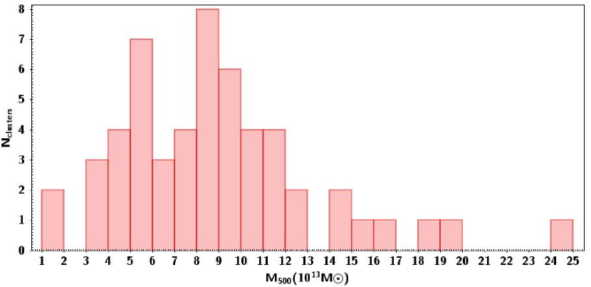
Figure 5: Histogram of the cluster masses within $R_{500}$, $M_{500}$, in units of $10^{13}$ M_⊙ computed from the X-ray data.

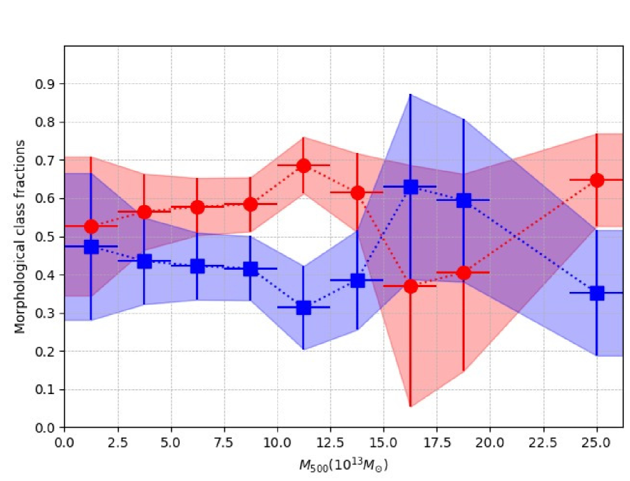
Figure 6: Fraction of early-type (red circles) and late-type (blue squares) as a function of cluster mass obtained after stacking the 54 clusters in mass bins.

The histogram of the cluster masses within $R_{500}$, $M_{500}$, is shown in Fig. 5. We compute the fractions of early and late-type galaxies in ten $M_{500}$ mass bins and show the corresponding results in Fig. 6. For each bin in cluster mass (and later distance to the cluster centre) in Fig. 6 (and later Fig. 7), the error bars are calculated considering Poisson distributions, hence as $\sqrt{N}/N$, where $N$ is the number of galaxies in each bin. No strong variation is observed, except perhaps for the most massive clusters, where there seems to be a somewhat larger fraction of late-type galaxies in the range $15\times 10^{13}<{\rm M}_{500}<20\times 10^{13}$ M_⊙. However, since this is not the case in the bin corresponding to the highest mass, it is difficult to say if there is a general trend and to give an interpretation.

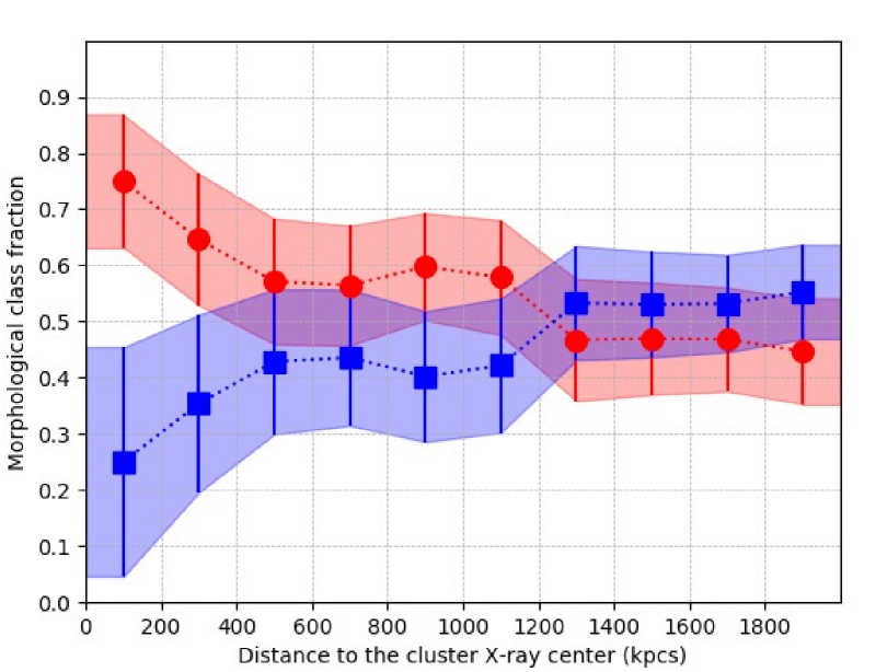
Figure 7: Fraction of early-type (red circles) and late-type (blue squares) as a function of distance to the cluster center obtained after stacking the 54 clusters in ten bins.

The fractions of early and late type galaxies were also computed as a function of cluster radius (in ten bins). The results are shown in Fig. 7. As expected, the fraction of early types is very large (close to 80%) in the innermost bins and decreases down to $\sim$50% around 1.3 Mpc, while the fraction of late types increases with radius and becomes larger than 50% around 1.3 Mpc.

A certain amount of contamination by foreground and background galaxies must occur when considering the fractions of early and late type galaxies. We estimated this contamination by comparing the red sequence galaxy counts in each magnitude bin and the corresponding background counts from the COSMOS survey, as estimated in Section 5 to compute GLFs. Values of the contamination vary from one cluster to another between 30% and 70% at a magnitude of $r^{\prime}\sim 20$ with no obvious dependence on redshift or on the M₅₀₀ cluster mass. The signal dilution due to contamination is expected to be stronger for low mass clusters, for which the contrast above the field is lower. This could explain our finding that low mass poor systems (Fig. 6) or cluster outermost parts (Fig. 7) have early to late type fractions comparable to those of the field.

We also tried to analyse the variations of the fractions of early and late types as a function of the number of galaxies within $R_{200}$ but found no significant result. Neither did we find any significant variation of the fractions of early and late types with redshift.

5 The galaxy luminosity functions of cluster galaxies

5.1 The method

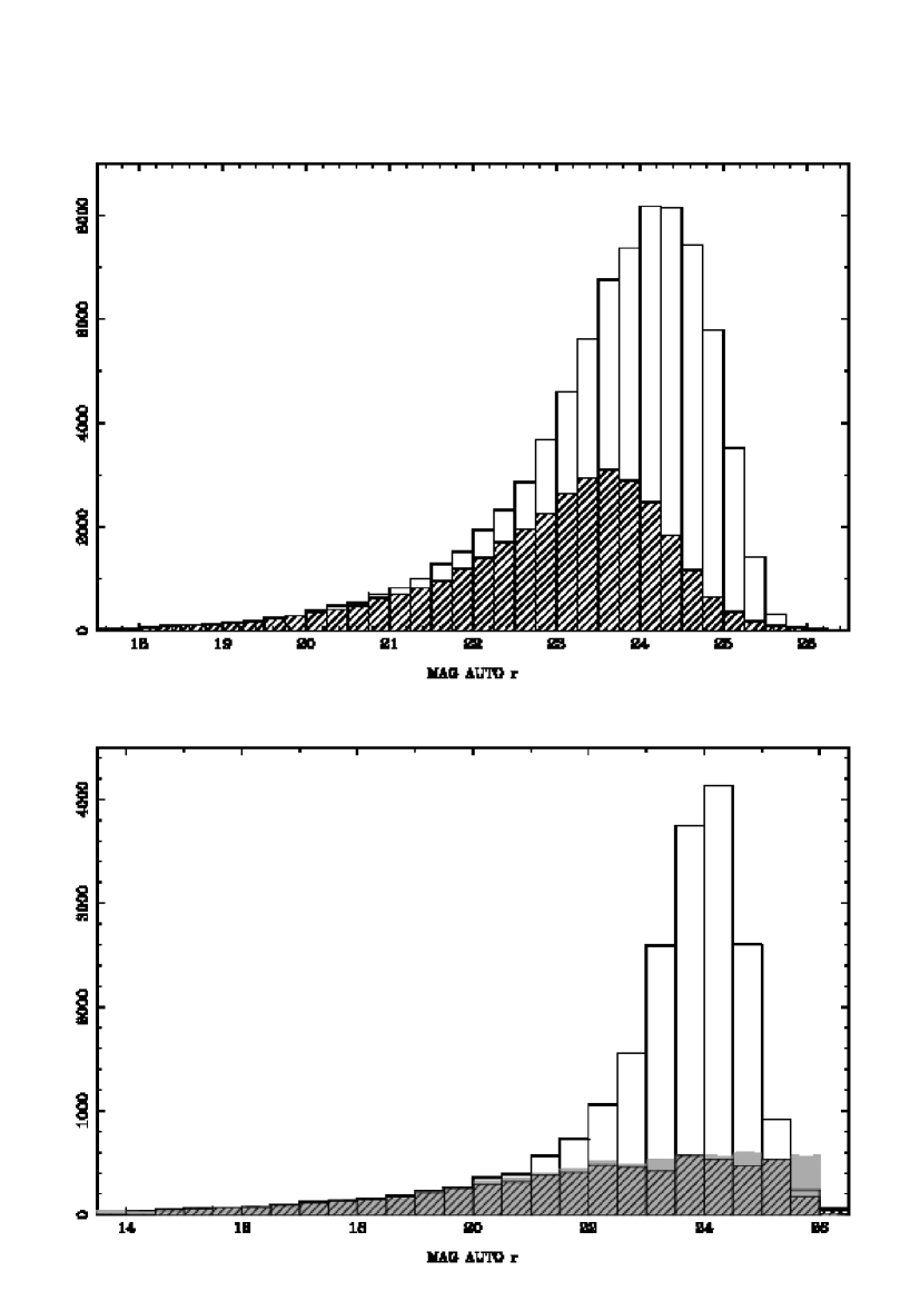
Figure 8: Top: galaxy magnitude histogram in the r band from the IAC catalogue (hatched) and from our catalogue (white) for cluster 3XMM J001737.3-005240. Bottom: star magnitude histogram in the r band from the IAC catalogue (white), from our catalogue (hatched) and from the Besançon model counts (grey) for cluster 3XMM J001737.3-005240.

We derive the galaxy luminosity functions (GLFs) of the 51 clusters with spectroscopic redshifts from our sample. We first test the quality of the Fliri & Trujillo (2016) catalogues. For this, we retrieve for one cluster (3XMM J001737.3$-$005240) the galaxy catalogue by Fliri & Trujillo (2016) in the cluster area and compare it to the one we obtain with our own method, where we optimize the extraction parameters (see description below). The result is that with our method we detect more faint galaxies above $r\sim 21$. This is illustrated by Fig. 8. The top figure shows the galaxy magnitude histogram in the r band from the IAC catalogue and from our catalogue extracted as described below for cluster 3XMM J001737.3-005240. We can see that above $r\sim 21$ we start detecting more galaxies. This seems due to a difference in galaxy–star separation between the two methods. As a comparison, we plot in the bottom figure the star magnitude histogram in the r band from the IAC catalogue, from our catalogue and from the Besançon model counts (Robin et al., 2003) for cluster 3XMM J001737.3$-$005240. We can see that our star counts match well those of the Besançon model, while the star counts from Fliri & Trujillo (2016) are much higher at faint magnitudes. Since our aim here is to go as deep as possible to measure the faint end slope of the galaxy luminosity functions, we decide to reextract catalogues from the images that we had already retrieved for the morphological analysis (see previous Section). This should be considered as a caveat to future users of the Fliri & Trujillo (2016) catalogues.

As described in the previous section, the images are retrieved in the five SDSS bands, plus rdeep. We make detections with SExtractor (Bertin & Arnouts, 1996) in the rdeep band, then measure magnitudes (MAG_AUTO) in dual image mode, using rdeep as a reference. The photometric zero points are calculated by applying Eq. (7) from Fliri & Trujillo (2016). For some clusters, it was necessary to mask some areas covered by very bright stars (and even one bright foreground galaxy). We then separate stars from galaxies based on a maximum surface brightness versus magnitude diagram (Jones et al., 1991). We always check that the histogram of the number of objects classified as stars is consistent with the number of stars predicted in the cluster direction by the Besançon model quoted above.

For each cluster, we apply the following steps. We limit our analysis to galaxies within the $R_{200}$ radius of each cluster, for two reasons. First, this value is chosen to increase the contrast over the background, and second it allows to separate better clusters that are close in projection on the sky. The red sequence (RS) is defined based on a colour-magnitude diagram. In order to bracket the 4000 Å break, we choose different colour-magnitude diagrams for different cluster redshift ranges: $g-r$ versus $r$ for $0<z<0.43$, $r-i$ versus $i$ for $0.43\leq z\leq 0.70$ and $i-z$ versus $z$ for $z>0.70$ (Hao et al., 2010). Galaxies with spectroscopic redshifts within 0.01 of the cluster redshift and with photometric redshifts within $\pm 0.04(1+z_{cluster})$ are superimposed on the colour-magnitude diagrams to define better the RS. The slope of the colour-magnitude relation is fixed to $-0.0436$ (as e.g. in Martinet et al., 2015). A first estimation is made by eye. We then select all galaxies within $\pm 0.6$ of this fit to compute the best fit to the colour-magnitude relation, and we keep all the galaxies within $\pm 0.3$ of this best fit (see e.g. in De Lucia et al., 2007) to compute the GLF.

The subtraction of the background galaxy contribution is made using the COSMOS catalogue of Laigle et al. (2016), which covers a region of 1.38 deg², more than 10 times larger than the zones covered by our clusters. Magnitudes from the COSMOS catalogue (Subaru filters) are transformed into SDSS magnitudes with LePhare (Arnouts et al., 1999; Ilbert et al., 2006), with extinction laws by Calzetti & Heckman (1999) and emission lines from Polletta et al. (2006). We then extract for each cluster the COSMOS background counts corresponding to the same extraction around the RS as for cluster galaxies, normalize all the counts to 1 deg² and make count histograms in bins of 0.5 magnitudes. This is done in all five bands, u, g, r, i and z.

Table 2: 90% and 80% completeness limits for the detections of extended sources in the five bands considered. The last line gives the completeness limits of the SDSS Stripe 82 data given by Annis et al. (2014).

filter	u	g	r	i	z
90%	22.9	23.5	23.1	22.6	21.7
80%	23.1	23.8	23.6	22.9	22.0
Annis 90%	23.1	22.8	22.4	22.1	20.4

Before analysing GLFs, we estimate the completeness levels reached in each band. This is done through point source simulations as in Martinet et al. (2015). The completeness limits for extended sources are about 0.5 magnitudes brighter than for point sources (Adami et al., 2007). We compute GLFs within the 90% and 80% completeness limits given in Table 2. We also give in this Table the 90% completeness limits of the SDSS Stripe 82 given by Annis et al. (2014). We can note that except in the u band the data extracted from Fliri & Trujillo (2016) appear deeper, thus justifying our choice.

Finally, apparent magnitudes $m$ are converted to absolute magnitudes $M$ using the usual formula:

$$M=m-5(\log_{10}D_{L}-1)-kcor$$ (4)

where $D_{L}$ is the luminosity distance (in pc) computed with Ned Wright’s cosmology calculator and $kcor$ is the k-correction. For each cluster, we compute $kcor$ with LePhare as the average value for all the elliptical galaxy templates with a redshift within $\pm 0.05$ of the cluster redshift.

The error bars on the galaxy counts are computed as follows. We consider that the errors on the counts along the red sequence (RS) $N_{RS}$ and the field counts $N_{bkg}$ are poissonian. The GLF is defined by:

$$\tilde{N}=\tilde{N}_{RS}-\tilde{N}_{bkg}\mbox{,}$$ (5)

where $\tilde{N}_{RS}=\frac{N_{RS}}{A_{RS}}$ is the number of galaxies along the RS normalised to 1 deg² ($A_{RS}=\pi*R_{200}^{2}$ ) and $\tilde{N}_{bkg}=\frac{N_{bkg}}{A_{bkg}}$ is the number of background galaxies normalised to 1 deg² ($A_{bkg}=1.38$ deg² ).

The error on the galaxy counts normalised to 1 deg² is then:

$$\tilde{E}=\sqrt{\tilde{E}_{RS}^{2}+\tilde{E}_{bkg}^{2}}\mbox{,}$$ (6)

with $\frac{\tilde{E}_{RS}}{\tilde{N}_{RS}}=\frac{E_{RS}}{N_{RS}}=\frac{1}{\sqrt{N_{RS}}}$ and $\frac{\tilde{E}_{bkg}}{\tilde{N}_{bkg}}=\frac{E_{bkg}}{N_{bkg}}=\frac{1}{\sqrt{N_{bkg}}}$ (the relative errors remain the same).

The final error $\tilde{E}$ on the normalised GLFs for individual clusters is therefore:

$$\tilde{E}=\sqrt{\tilde{E}_{RS}^{2}+\tilde{E}_{bkg}^{2}}=\sqrt{\frac{\tilde{N}_{RS}}{A_{RS}}+\frac{\tilde{N}_{bkg}}{A_{bkg}}}=\sqrt{\frac{N_{RS}}{A_{RS}^{2}}+\frac{N_{bkg}}{A_{bkg}^{2}}}$$ (7)

We then fit the GLFs with a Schechter function:

$$\Phi(M)=0.4\ \ln(10)\Phi^{*}\times[10^{0.4(M^{*}-M)}]^{\alpha+1}\times\exp(-10^{0.4(M^{*}-M)})$$ (8)

where $\Phi^{*}$ is the normalisation factor, $M^{*}$ is the absolute magnitude where the regime changes from bright to faint galaxies and $\alpha$ is the faint end slope. The fit is made by minimizing a $\chi^{2}$ using the MINUIT routine.

GLFs are then stacked in mass and redshift bins to improve the quality of the fits and see if a trend can be found. For this, we follow the prescription developed by Colless (1989), where the clusters are normalised to the same solid angle (1 deg²) and to the same richness, defined as the number of galaxies in a given band up to a certain limiting magnitude, which we will take to be the 80% completeness limit (see Table 2). As discussed in e.g. Martinet et al. (2017), the Colless stack, although it allows to maximize the information from the available data as compared to a fixed number of clusters per bin, presents the caveat that the stack is dominated by the low-redshift clusters, since these tend to have a deeper completeness limit. The redshift bins used in this analysis are however sufficiently thin to study a possible evolution from $z=0.2$ to $z=0.5$. Following the prescription by Popesso et al. (2005), the galaxy number counts in bin $j$ of the stacked GLF are:

$$N_{sj}=\frac{N_{s0}}{Nc_{tot}Nc_{j}}\sum\limits_{i}\frac{\tilde{N_{ij}}}{N_{i0}}\mbox{,}$$ (9)

where $\tilde{N_{ij}}$ is the number of galaxies in bin $j$ for cluster $i$ normalised to 1 deg², $N_{i0}$ corresponds to the richness of cluster $i$, $N_{s0}$ is the sum of the richnesses of all the clusters:

$$N_{s0}=\sum\limits_{i}N_{i0}\mbox{,}$$ (10)

$Nc_{tot}$ is the total number of clusters in the stack and $Nc_{j}$ is the number of clusters contributing to bin $j$.

The error on $N_{sj}$ is obtained from the Poisson errors $\tilde{E_{ij}}$ (see above):

$$E_{sj}=\frac{N_{s0}}{m_{tot}m_{j}}\left[\sum\limits_{i}(\frac{\tilde{E_{ij}}}{N_{i0}})^{2}\right]^{(1/2)}\mbox{.}$$ (11)

The cluster richness is used as a normalisation for the stacks, allowing a direct comparison of the values of $\Phi^{*}$ from one stack to another.

5.2 Results

Individual GLFs are first computed for all the clusters, except for the three clusters that we eliminate because they only have photometric redshifts. Schechter fits are made for both completeness limits (90% and 80%), but since the results are not very different we choose to give the results only for the 80% completeness limit (for which the number of converging fits is slightly larger). The parameters of the Schechter fits for the individual clusters are given in Appendix C, Table C1. For three clusters, the GLF cannot be fit by a Schechter function in any band, so they do not appear in Table C1. For fifteen clusters, the individual GLF fits are of poor quality, with large error bars on the parameters. Out of these, six are distant ($z>0.65$), and three have one or several bright foreground galaxies close to the cluster center. The remaining six clusters are neither particularly distant nor massive, so the reason for the poor quality of the GLF fit is unclear. For most clusters the GLFs in the u band are too faint to allow a fit by a Schechter function, so this band will not be discussed.

We want to stress the fact that the minimization procedure used here to fit the GLFs with Schechter functions gives the $\Phi^{*}$, $M^{*}$ and $\alpha$ parameters with the error bars that we give in the various tables, but, as we have noted in many of our previous papers, these error bars are always underestimated. This must be kept in mind when comparing GLFs and trying to derive conclusions.

We discuss below the GLF Schechter parameters and show the corresponding figures for stacked clusters (in mass and redshift bins).

5.2.1 GLFs in mass bins

Table 3: GLF parameter fits of stacked galaxy luminosity functions for low mass ($M<7\ 10^{13}$ M_⊙), medium mass ($7\ 10^{13}\leq M\leq 10^{14}$ M_⊙), and high mass ($M>10^{14}$ M_⊙) clusters. Cols. 2–4 correspond to stacking all the clusters with converging fits (stack $a$) and Cols. 5–7 to stacking only the clusters for which the errors on the GLF fits are not too large (stack $b$). The numbers of clusters included in each stack are indicated in parentheses. In the two cases indicated with an asterisk, the fits do not converge since the values $M^{*}_{z}$ are at their limit value of $-26.0$.

	stack $a$			stack $b$
	Low mass (16)	Medium mass (16)	High mass (12)	Low mass (12)	Medium mass (14)	High mass (9)
$\Phi_{g}$		$260\pm 25$	$152\pm 19$		$223\pm 22$	$346\pm 46$
M${}^{*}_{g}$		$-23.6\pm 0.1$	$-25.6\pm 0.2$		$-23.7\pm 0.1$	$-23.6\pm 0.2$
$\alpha_{g}$		$-1.31\pm 0.02$	$-1.36\pm 0.02$		$-1.33\pm 0.02$	$-1.36\pm 0.02$
$\Phi_{r}$	$178\pm 106$	$304\pm 15$	$413\pm 38$	$150\pm 66$	$240\pm 17$	$663\pm 91$
M${}^{*}_{r}$	$-25.0\pm 1.5$	$-24.2\pm 0.1$	$-24.5\pm 0.1$	$-24.7\pm 0.7$	$-24.3\pm 0.1$	$-23.1\pm 0.1$
$\alpha_{r}$	$-1.24\pm 0.05$	$-1.29\pm 0.01$	$-1.21\pm 0.02$	$-1.38\pm 0.04$	$-1.32\pm 0.01$	$-1.22\pm 0.04$
$\Phi_{i}$	$413\pm 94$	$363\pm 16$	$647\pm 36$	$232\pm 68$	$258\pm 15$	$756\pm 66$
M${}^{*}_{i}$	$-23.7\pm 0.2$	$-24.0\pm 0.1$	$-24.0\pm 0.1$	$-24.4\pm 0.4$	$-24.4\pm 0.1$	$-23.4\pm 0.1$
$\alpha_{i}$	$-1.10\pm 0.06$	$-1.24\pm 0.01$	$-1.16\pm 0.02$	$-1.30\pm 0.04$	$-1.30\pm 0.01$	$-1.18\pm 0.02$
$\Phi_{z}$	$377\pm 110$	$152\pm 19$	$968\pm 57$	$124\pm 11^{*}$	$112\pm 5^{*}$	$1085\pm 106$
M${}^{*}_{z}$	$-24.0\pm 0.3$	$-25.6\pm 0.2$	$-23.9\pm 0.1$	$-26.0\pm 1.0^{*}$	$-26.0\pm 0.2^{*}$	$-23.3\pm 0.1$
$\alpha_{z}$	$-1.12\pm 0.08$	$-1.36\pm 0.02$	$-1.06\pm 0.02$	$-1.36\pm 0.03^{*}$	$-1.38\pm 0.01^{*}$	$-1.03\pm 0.04$

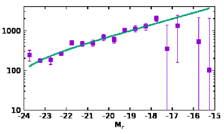
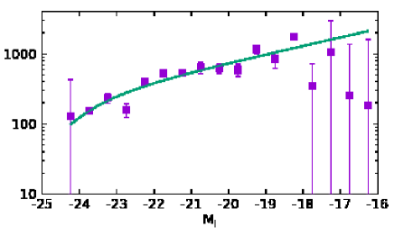
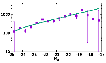
Figure 9: GLFs and Schechter fits for the stack of 12 low mass ($M<7\ 10^{13}$ M_⊙) clusters.

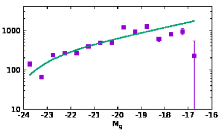
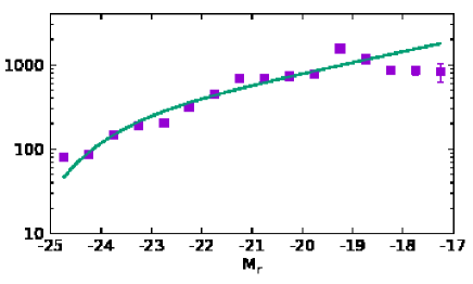
Figure 10: GLFs and Schechter fits for the stack of 14 medium mass ($7\ 10^{13}\leq M\leq 10^{14}$ M_⊙) clusters.

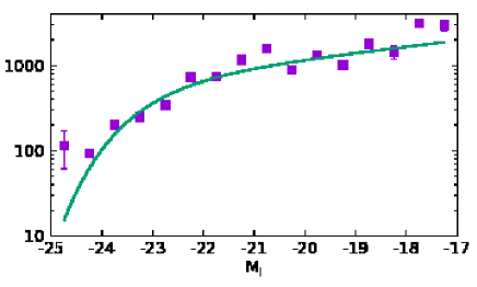
Figure 11: GLFs and Schechter fits for the stack of 9 high mass ($M>10^{14}$ M_⊙) clusters.

The histogram of cluster masses within $R_{500}$ has been shown in the previous Section. To see if we can detect a variation of the Schechter parameters with cluster mass, we divide our sample into three mass bins: low mass ($M<7\ 10^{13}$ M_⊙), medium mass ($7\ 10^{13}\leq M\leq 10^{14}$ M_⊙), and high mass ($M>10^{14}$ M_⊙) clusters. We first include in stack $a$ all the clusters with converging Schechter fits (44 clusters). These are distributed as follows: 16 low mass, 16 medium mass and 12 high mass clusters. We then try including in stack $b$ only the 35 clusters with Schechter fits that do not show too large error bars. This gives 12 low mass, 14 medium mass and 9 high mass clusters. Clusters belonging to these two stacks are respectively noted with superscripts $a$ and $b$ in Table LABEL:tab:Sch_param_all.

The Schechter fit parameters for the stacks in mass bins are given in Table 3 and the corresponding GLFs are shown in Figs. 9, 10 and 11. We can note that the Schechter fit parameters are very similar (within error bars) for the two different stacks for medium and high mass clusters. They differ a little more for low mass clusters, but these differences are not statistically significant.

This implies that the GLF fits remain comparable even when a few clusters with low signal to noise are included, a rather comforting result. We do not give the Schechter parameters in the g band for low mass clusters because they do not converge. For low and medium mass clusters of stack $b$, we give the Schechter parameters in the z band as an indication, because the GLFs obtained are “reasonable” (see the bottom of Figs. 9 and 10) but the $M^{*}$ parameters are at their limits of $-26.0$, so the fits are not reliable. All the other fits converge, but we must keep in mind the fact that the error bars on the Schechter parameters are probably underestimated by a factor between 1 and 1.5, based on our previous experience. Variance from one cluster to another induces variations in the Schechter fit parameters, and since there are between 9 and 16 clusters in our stacks the uncertainties on the parameters are larger than if we were stacking hundreds of clusters (see for example the error bars in the Tables of Appendix C in Sarron et al., 2018).

For high mass clusters, which are the most reliable, we can see that the faint end slope $\alpha$ clearly varies with the photometric band: it smoothly flattens from g to z. This has already been noted for other clusters such as Coma (see e.g. Adami et al., 2007, Fig. 13). Besides this trend, it is difficult to claim any other significant variation of Schechter fit parameters (given in Table 3) with cluster mass.

The absence of a variation of the GLF with cluster mass was already noted in the extensive study of cluster GLFs made by Sarron et al. (2018), based on a catalogue of 1371 cluster candidates in the Canada France Hawaii Telescope Legacy Survey (see their Fig. B.2). These authors found that it is only when blue and red galaxies are separated that the GLFs of blue and red galaxies start showing differences with cluster mass. Here, we are only studying red galaxies, but our cluster sample is much smaller than that of Sarron et al. (2018), so we cannot reach a definite conclusion on the variation of Schechter fit parameters with cluster mass.

5.2.2 GLFs in redshift bins

The histogram of cluster redshifts is shown in Fig. 1. There are 12 clusters with redshifts $z>0.5$, but for two of them the galaxy counts are barely above the background so we could not fit the GLFs and we decided not to include them in the stack. We therefore stack the ten remaining clusters (noted with a ^c in Table LABEL:tab:Sch_param_all) to compute the “high redshift” GLF. As a comparison, we stack ten low redshift clusters with redshifts $0.2<z<0.3$ to constitute the “low redshift” GLF. These ten clusters were chosen to have a mass distribution as close as possible as the high redshift sample, to avoid introducing a possible influence of the cluster mass on the comparison between high and low redshift clusters.

The results are given in Table 4 for the r, i and z bands (at high redshift, the fit to the stacked GLF in the g band does not converge). To avoid including too many figures, we are not showing the corresponding GLFs, since they are quite similar to those given in the previous subsection.

We can see that the faint end slope is flatter at high redshift in the r and z bands, but not in the i band, so it is difficult to reach any definite conclusion. A small trend of a flattening faint end slope was also found by Sarron et al. (2018), as seen in their Fig. 12, but here also the trend is stronger for blue galaxies, and since we are only studying the GLFs of red galaxies here, we cannot draw firm conclusions on the variation of GLF parameters with redshift.

Table 4: GLF best fit parameters of stacked galaxy luminosity functions for 10 low redshift ($0.2<z<0.3$) and 10 high redshift ($z>0.5$) clusters.

	Low redshift (10)	High redshift (10)
$\Phi_{r}$	$333\pm 43$	$1717\pm 75$
M${}^{*}_{r}$	$-23.1\pm 0.1$	$-23.3\pm 0.04$
$\alpha_{r}$	$-1.26\pm 0.03$	$-0.92\pm 0.03$
$\Phi_{i}$	$392\pm 45$	$715\pm 48$
M${}^{*}_{i}$	$-23.3\pm 0.2$	$-24.8\pm 0.1$
$\alpha_{i}$	$-1.18\pm 0.03$	$-1.24\pm 0.01$
$\Phi_{z}$	$263\pm 37$	$1481\pm 67$
M${}^{*}_{z}$	$-24.2\pm 0.2$	$-23.68\pm 0.05$
$\alpha_{z}$	$-1.19\pm 0.04$	$-0.98\pm 0.03$

6 Conclusions

We have presented a detailed analysis of the cluster sample published from our cluster survey, the 3XMM/SDSS Stripe 82 galaxy cluster survey. Our study includes 54 clusters in a redshift range from 0.05 to 1.2 (51 spectroscopic redshifts and 3 photometric redshifts).

We first determined the X-ray temperatures and luminosities of 45 clusters through spectral fitting of their spectra, in an aperture of 300 kpc. The X-ray data quality of the remaining systems did not allow a spectral analysis. The X-ray temperatures are in the range [1.0-8.0] keV and the X-ray luminosities in an aperture of radius 300 kpc are in the range [1.0-104]$10^{42}$ erg s^-1. For 37 clusters with good quality X-ray data, we investigated the ${\rm L_{X}-T_{X}}$ relation, and found a best fit slope of $3.01\pm 0.51$, similar to values published in the literature. We also found a good agreement between the intercept of our relation with those values derived for other relations based on different cluster samples. This shows that our sample is representative of typical cluster samples, with no obvious bias.

We then investigated some optical properties of the cluster galaxies. First, we computed the fraction of early and late type galaxies as a function of cluster mass and distance to the cluster X-ray centre. We observe no strong variation of the fraction of early and late type galaxies with cluster mass, except for the most massive clusters, which contain a somewhat larger fraction of late-type galaxies. This may be explained by the fact that more massive clusters accrete more late-type galaxies in their outskirts. As expected, we found a very large (close to 80%) fraction of early type galaxies in the innermost radial bin, decreasing to 50% at radii above 1.3 Mpc, while the fraction of late type galaxies increases with radius and becomes larger than 50% around 1.3 Mpc. We found no significant variations of the fractions of early and late type galaxies as a function of the number of galaxies within $R_{200}$.

Second, we investigated the galaxy luminosity functions (GLFs) in the five ugriz bands for red sequence selected galaxies. We limited our study of the individual GLFs to 36 clusters. For the few clusters with GLF fits in the $u$ band, the faint end slope tends to be steeper than in the other bands, a trend already noted in other studies (e.g. Boué et al., 2008, and references therein). However, in view of the large error bars on the Schechter parameters in the $u$ band, it is difficult to confirm this trend. For a given cluster, the faint end slopes in the other bands are all similar within the error bars.

We then stacked the GLFs in the griz bands in three mass bins and two redshift bins. The Schechter fit parameters are very similar for the stacks for medium and high mass clusters. They are slightly different for low mass clusters, but this may just be due to the lower quality of the GLF fits for low mass clusters. For high mass clusters (the most reliable), the faint end slope varies with the photometric band, smoothly flattening from g to z, as previously noted for other clusters such as Coma Adami et al. (2007). Besides this trend, and keeping in mind the fact that the error bars on the Schechter parameters are most probably underestimated, it is difficult to claim any significant variation of Schechter fit parameters with cluster mass, in agreement with Sarron et al. (2018).

The comparison of the GLFs stacked in two redshift bins with comparable mass distributions shows that the faint end slope is flatter at high redshift ($z>0.5$) in the r and z bands, but not in the i band, so it is difficult to reach any definite conclusion on the variation with redshift, also in agreement with Sarron et al. (2018).

Twenty clusters of the present sample are studied for the first time in X-rays, and the 54 clusters of this sample are studied for the first time in the optical range. Altogether, our cluster sample appears to have X-ray and optical properties which are representative of “average” cluster properties, and can therefore be added to other cluster samples to increase, for example, the statistics on X-ray or optical cluster properties.

Appendix A X-ray parameters for the cluster sample used in the ${\rm L_{X}-T_{X}}$ relation

The X-ray parameters of our galaxy cluster sample are measured from spectral fits to cluster spectra extracted from XMM-Newton EPIC (MOS1, MOS2, pn) observations. Table 5 lists the X-ray parameters of the 37 systems used to investigate the ${\rm L_{X}-T_{X}}$ relation. The table columns are: DETID: Detection number in the 3XMM-DR5 catalogue, 3XMM Name: IAU name of the X-ray source, RA: right ascension of X-ray detection in degrees (J2000), Dec: declination of detection in degrees (J2000), OBSID: XMM observation identification number, z: galaxy cluster redshift (note: all the clusters of the sample have spectroscopic redshifts except for 3XMM J213340.8-003841 that has only a photometric redshift), $R_{300~{}kpc}$: spectrum extraction radius (300 kpc) in arcsec, $R_{500}$ radius in arcsec computed in the present work (see Section 3.2), nH: Galactic hydrogen column density, kT: X-ray temperature in [0.5-2.0] keV within $R_{300~{}kpc}$, nekT and pekT: negative and positive errors on kT, ekT: average error on kT, Lx: aperture ($R_{300~{}kpc}$) X-ray luminosity in [0.5-2.0] keV ($10^{42}$ erg s^-1), neLx and peLx: negative and positive errors in Lx, eLx: average error on Lx, $L_{500}$ and $eL_{500}$: X-ray bolometric luminosity and its error within $R_{500}$ ($10^{42}$ erg s^-1).

Table 5: X-ray parameters of our galaxy cluster sample (37 systems) that are used to plot the ${\rm L_{X}-T_{X}}$ relation.

DETID	3XMM name	RA	Dec	OBSID	z	$R_{300~{}kpc}$	$R_{500}$	nH	kT	nekT	pekT	ekT	Lx	neLx	peLx	eLx	$L_{500}$	$eL_{500}$
104037603010094	J001115.5+005152	2.81470	0.86462	0403760301	0.3622	59.4	93.3	0.027	2.32	0.51	0.85	0.68	3.3	0.4	0.5	0.5	9.0	1.1
102036901010028	J003838.0+004351	9.65851	0.73108	0203690101	0.6955	42.1	77.0	0.020	4.50	0.99	1.45	1.22	22.2	1.7	1.9	1.8	83.2	5.6
102036901010085	J003840.3+004747	9.66813	0.79659	0203690101	0.5553	46.6	82.0	0.020	3.05	0.77	1.09	0.93	12.4	1.4	1.3	1.3	38.2	3.0
102036901010023	J003922.4+004809	9.84359	0.80277	0203690101	0.4145	54.7	108.1	0.020	3.79	0.51	0.52	0.52	12.5	0.6	0.6	0.6	45.9	1.0
102036901010017	J003942.2+004533	9.92597	0.75926	0203690101	0.4156	54.6	104.4	0.019	2.36	0.32	0.35	0.34	13.5	0.9	0.7	0.8	37.5	1.3
100900702010087	J004231.0+005112	10.62930	0.85336	0090070201	0.1579	110.0	182.3	0.018	1.70	0.16	0.21	0.18	2.5	0.2	0.2	0.2	6.1	0.4
100900702010056	J004252.5+004300	10.71892	0.71692	0090070201	0.2697	72.6	133.8	0.018	2.63	0.48	0.75	0.61	5.8	0.5	0.4	0.5	17.3	1.1
100900702010050	J004334.1+010107	10.89187	1.01811	0090070201	0.2000	90.9	172.6	0.018	1.60	0.10	0.09	0.09	7.0	0.4	0.4	0.4	16.3	0.7
100900702010052	J004350.6+004731	10.96114	0.79216	0090070201	0.4754	50.5	100.4	0.018	3.76	0.70	1.13	0.92	17.1	1.3	1.5	1.4	59.6	3.6
103035622010028	J004401.4+000644	11.00583	0.11226	0303562201	0.2187	84.8	182.4	0.017	2.59	0.46	0.67	0.56	12.2	0.9	1.1	1.0	37.8	1.5
103031104010030	J005546.1+003839	13.94249	0.64422	0303110401	0.0665	235.3	403.3	0.028	1.30	0.05	0.05	0.05	2.6	0.2	0.1	0.1	5.6	0.2
106053911010001	J012023.3-000444	20.09717	-0.07908	0605391101	0.0780	203.3	438.2	0.034	1.64	0.03	0.03	0.03	9.6	0.1	0.2	0.2	24.1	0.5
101016402010005	J015917.1+003010	29.82144	0.50300	0101640201	0.3820	57.4	161.2	0.023	2.91	0.33	0.31	0.32	104.3	3.5	3.9	3.7	360.2	8.5
101016402010018	J020019.2+001932	30.08002	0.32564	0101640201	0.6825	42.4	84.3	0.023	1.90	0.25	0.38	0.31	58.5	6.8	7.8	7.3	132.8	15.1
106524006010012	J022825.8+003203	37.10780	0.53441	0652400601	0.3952	56.3	125.5	0.023	3.40	0.25	0.39	0.32	26.2	0.8	0.9	0.9	90.4	0.3
106524006010017	J022830.5+003032	37.12738	0.50907	0652400601	0.7214	41.5	85.2	0.023	6.31	1.07	1.69	1.38	38.4	2.2	2.9	2.5	188.9	11.9
106524007010008	J023026.7+003733	37.61157	0.62602	0652400701	0.8600	39.0	83.5	0.021	7.96	1.46	2.56	2.01	72.4	3.7	3.9	3.8	419.5	9.2
106064313010011	J025846.5+001219	44.69388	0.20555	0606431301	0.2589	74.8	167.7	0.065	3.73	0.95	1.53	1.24	14.2	1.4	1.4	1.4	56.8	3.7
106064313010004	J025932.5+001353	44.88574	0.23161	0606431301	0.1920	93.9	223.2	0.067	3.43	0.58	0.85	0.71	16.6	1.1	1.1	1.1	64.5	1.6
100411701010097	J030145.7+000323	45.44072	0.05659	0041170101	0.6900	42.2	67.0	0.070	1.71	0.32	0.98	0.65	15.0	2.5	4.7	3.6	33.4	7.5
100411701010074	J030212.1-000132	45.55054	-0.02579	0041170101	1.1900	36.2	53.3	0.071	3.87	0.69	0.98	0.84	33.1	3.2	3.3	3.2	140.0	13.2
100411701010113	J030212.1+001107	45.55082	0.18536	0041170101	0.6523	43.2	59.6	0.069	1.83	0.25	0.57	0.41	5.4	0.8	1.5	1.1	12.0	2.6
100411701010112	J030317.5+001245	45.82296	0.21272	0041170101	0.5900	45.2	66.4	0.068	1.58	0.27	0.30	0.28	7.0	1.1	1.2	1.1	14.1	2.3
101426101010024	J030614.1-000540	46.55923	-0.09474	0142610101	0.4249	53.9	103.0	0.063	2.15	0.23	0.31	0.27	14.0	0.7	1.3	1.0	38.9	1.9
101426101010022	J030617.3-000836	46.57206	-0.14361	0142610101	0.1093	150.5	268.5	0.064	1.68	0.08	0.25	0.16	3.4	0.1	0.2	0.2	8.2	0.2
101426101010059	J030633.1-000350	46.63804	-0.06408	0142610101	0.1235	135.3	193.4	0.063	1.46	0.12	0.16	0.14	1.1	0.1	0.1	0.1	2.2	0.2
102011201010042	J030637.3-001801	46.65570	-0.30054	0201120101	0.4576	51.6	90.9	0.063	2.54	0.51	0.82	0.66	8.9	1.3	1.5	1.4	26.3	3.5
104023202010027	J033446.2+001710	53.69279	0.28618	0402320201	0.3261	63.6	130.1	0.070	2.49	0.47	0.92	0.70	13.3	1.5	2.4	1.9	40.7	4.2
101349209010028	J035416.9-001003	58.57060	-0.16751	0134920901	0.2100	87.5	190.9	0.117	4.60	1.05	1.68	1.37	7.8	0.6	0.8	0.7	40.1	2.4
103048012010021	J213340.8-003841	323.41996	-0.64481	0304801201	0.2110	87.2	197.3	0.036	3.60	0.50	0.67	0.59	13.4	0.6	0.8	0.7	50.6	1.4
106553468400021	J221211.0-000833	333.04618	-0.14275	0655346840	0.3643	59.2	119.6	0.044	3.60	0.49	2.41	1.45	17.1	2.1	2.6	2.4	43.4	4.8
106553468390009	J221422.1+004712	333.59226	0.78680	0655346839	0.3202	64.4	132.2	0.035	4.28	1.28	2.17	1.72	9.9	1.6	1.5	1.6	40.7	5.2
106700202010013	J222144.0-005306	335.43347	-0.88513	0670020201	0.3353	62.5	119.8	0.047	2.10	0.38	0.48	0.43	10.6	1.0	1.7	1.4	28.2	2.4
106524010010043	J232809.0+001116	352.03771	0.18778	0652401001	0.2780	71.1	125.9	0.041	3.25	0.72	1.40	1.06	4.1	0.4	0.3	0.3	14.0	1.0
106524011010056	J232925.6+000554	352.35668	0.09849	0652401101	0.4021	55.7	86.4	0.041	2.35	0.51	0.93	0.72	3.6	0.4	0.5	0.4	9.7	1.1
106524014010034	J233138.1+000738	352.90912	0.12725	0652401401	0.2238	83.4	138.0	0.041	1.30	0.04	0.04	0.04	3.9	0.1	0.2	0.2	7.5	0.2
106524013010039	J233328.1-000123	353.36739	-0.02308	0652401301	0.5120	48.5	94.3	0.039	6.14	1.85	2.92	2.39	11.8	1.4	1.4	1.4	59.7	6.1

Appendix B Brightest cluster galaxies (BCGs)

We give in Table 6 the list of the BCGs for 53 of our 54 clusters with their positions, spectroscopic and photometric redshifts, and magnitudes in the five bands (we could not identify the BCG of cluster 3XMM J030637.3-001801).

Table 6: List of BCGs for 53 clusters. The columns are: 1) cluster name, 2) and 3) RA and Dec (J2000.0) of the BCG, 4) spectroscopic redshift (zspec), 5) photometric redshift (zphot), 6)  to 10) observed magnitudes in the u, g, r, i, and z bands. Quantities that could not be measured are noted as 99.99.

Cluster (3XMM)	RA	Dec	zspec	zphot	u	g	r	i	z
J001115.5+005152	2.81328	0.86553	0.36470	0.39719	99.990	20.416	18.327	17.911	16.970
J001737.3-005240	4.40162	-0.91354	0.21677	0.19107	20.755	19.043	17.721	17.014	16.986
J002223.3+001201	5.59128	0.19003	0.27911	0.26268	99.990	19.392	17.838	17.293	16.971
J002314.4+001200	5.81153	0.19945	0.25966	0.25256	22.045	19.011	17.492	17.064	16.810
J002928.6-001250	7.36553	-0.19710	0.06859	0.08381	19.606	18.344	18.018	17.809	17.751
J003838.0+004351	9.65987	0.73585	0.69818	0.90131	99.990	99.990	20.210	19.062	18.580
J003840.3+004747	9.67856	0.81097	99.99000	0.54099	99.990	22.280	21.291	20.941	99.990
J003922.4+004809	9.84172	0.80543	0.41833	0.38856	99.990	21.115	19.169	18.456	18.197
J003942.2+004533	9.93734	0.73325	0.41513	0.37082	99.990	21.538	19.790	19.062	18.781
J004231.0+005112	10.60627	0.86424	0.16679	0.11600	19.680	18.186	17.479	17.124	16.918
J004252.5+004300	10.60627	0.86424	0.16679	0.11600	99.990	99.990	17.479	99.990	99.990
J004334.1+010107	10.83817	0.99669	0.19777	0.18827	99.990	18.418	17.064	16.613	16.311
J004350.6+004731	10.95829	0.78839	0.47578	0.48996	99.990	21.569	19.451	18.496	18.250
J004401.4+000644	11.00534	0.11337	0.21971	0.22075	21.353	18.718	17.058	16.732	16.571
J005546.1+003839	13.93826	0.65065	0.06991	0.08277	19.733	18.247	17.202	17.043	16.808
J005608.9+004106	14.01921	0.64810	0.06961	0.08748	20.245	18.433	17.542	17.192	17.000
J010606.7+004925	16.55266	0.87025	0.26546	0.27514	99.990	19.558	18.084	17.686	17.368
J010610.0+005108	20.08572	-0.08110	0.08188	0.10104	20.725	18.602	17.637	17.288	17.002
J012023.3-000444	29.82316	0.51869	0.38400	0.37363	22.979	20.848	19.051	18.524	18.114
J015917.1+003010	29.95954	0.27864	99.99000	0.77416	99.990	22.424	22.142	21.407	99.990
J015953.1+001659	30.08100	0.32492	0.68247	0.43936	99.990	22.433	20.406	18.922	18.787
J020019.2+001932	32.55104	-0.24733	0.28275	0.25294	99.990	19.108	17.678	17.143	16.835
J021012.6-001439	32.72601	-0.39254	0.31787	0.32762	99.990	20.050	18.347	17.764	17.485
J021045.8-002156	37.12971	0.52598	0.40177	0.66653	21.015	20.748	20.101	19.653	19.256
J022825.8+003203	37.12971	0.52598	0.40177	0.66653	21.015	20.748	20.101	19.653	19.256
J022830.5+003032	37.61845	0.59797	99.99000	0.87046	99.990	24.132	23.021	99.990	99.990
J023026.7+003733	37.74370	0.73723	0.47402	0.48463	99.990	22.888	21.162	20.461	19.997
J023058.5+004327	44.66437	0.16252	0.26216	0.23974	99.990	19.764	18.490	17.952	17.629
J025846.5+001219	44.87015	0.26878	0.19441	0.27494	23.168	20.798	19.517	19.061	18.688
J025932.5+001353	45.42060	0.05867	99.99000	0.73122	99.990	99.990	22.804	21.525	20.901
J030145.7+000323	45.52695	-0.00764	99.99000	0.68029	99.990	99.990	22.419	21.245	99.990
J030205.6-000001	45.57111	-0.03033	99.99000	0.69769	99.990	99.990	21.700	19.924	19.354
J030212.1-000132	45.54819	0.18750	0.65228	0.64433	99.990	99.990	20.707	19.431	19.280
J030212.1+001107	45.82090	0.20803	0.60487	0.58124	99.990	22.174	20.454	19.204	18.898
J030317.5+001245	46.55886	-0.09439	0.42488	0.38512	99.990	20.605	18.797	18.033	17.666
J030614.1-000540	46.63088	-0.23376	0.11949	0.12933	19.872	17.787	16.824	16.384	16.064
J030617.3-000836	46.66190	-0.04452	0.11252	0.17952	99.990	20.712	19.831	19.327	19.004
J030633.1-000350	46.66190	-0.04452	0.11252	0.17952	99.990	99.990	19.831	99.990	99.990
J033446.2+001710	53.71614	0.25407	0.32789	0.29340	99.990	20.378	18.895	18.209	18.020
J035416.9-001003	58.52259	-0.15527	0.21438	0.20863	99.990	20.755	19.076	18.419	17.936
J213340.8-003841	323.41968	-0.59219	99.99000	0.24568	99.990	22.762	21.722	21.430	99.990
J221211.0-000833	333.02767	-0.10111	0.36528	0.36263	99.990	20.927	18.919	18.194	17.981
J221422.1+004712	333.59307	0.78494	0.32024	0.34345	99.990	19.605	17.856	17.258	16.945
J221449.2+004707	333.70879	0.74090	99.99000	0.35645	99.990	23.189	22.581	21.985	21.409
J221722.9-001013	334.35941	-0.17238	0.33220	0.33786	99.990	20.406	18.675	18.013	17.525
J222144.0-005306	335.42355	-0.88732	0.33658	0.39220	99.990	21.905	20.045	19.410	19.083
J232540.3+001447	351.42001	0.24385	99.99000	0.74049	99.990	23.706	23.087	22.301	99.990
J232613.8+000706	351.58764	0.11234	0.42613	0.42201	99.990	21.114	19.284	18.539	18.382
J232742.1+001406	351.92704	0.22466	0.44513	0.44309	99.990	22.439	20.476	19.492	19.364
J232809.0+001116	352.01612	0.15310	0.28008	0.29981	21.943	20.707	19.847	19.497	19.188
J232925.6+000554	352.35567	0.09943	0.40193	0.38233	99.990	21.017	18.961	18.170	18.104
J233138.1+000738	352.90866	0.12840	0.22382	0.22896	22.171	18.802	17.398	16.746	16.720
J233328.1-000123	353.36624	-0.02276	0.51201	0.52293	99.990	21.227	19.387	18.469	18.099

Appendix C Schechter fit parameters for individual clusters

The parameters of the Schechter fits up to the 80% completeness level are given in Table LABEL:tab:Sch_param_all for all the analysed clusters for which the GLFs converge. To make this table more readable, we also choose to give the $M^{*}$ and $\alpha$ parameters, but not the normalisation parameter $\Phi$, which is not very informative, since it is usually not well constrained. All the clusters except one (noted with an asterisk) are included in the GLF stacks in mass. The clusters indicated with a $z$ superscript are those included in the GLF stacks in redshift.

Table 7: Schechter parameters $M^{*}$ and $\alpha$ for the 36 individual clusters for which the fits have converged in at least one band.

Cluster (3XMM)	z	R200	M500	$M^{*}_{u}$	$\alpha_{u}$	$M^{*}_{g}$	$\alpha_{g}$	$M^{*}_{r}$	$\alpha_{r}$	$M^{*}_{i}$	$\alpha_{i}$	$M^{*}_{z}$	$\alpha_{z}$
		(kpc)	($10^{13}$ M⊙)
J001115.5+005152	0.3622	729.8	4.78							$-22.8\pm 2.0$	$-1.26\pm 0.51$	$-23.2\pm 2.6$	$-0.97\pm 0.72$
J001737.3-005240	0.2141	1120.1	14.67	$-19.8\pm 1.6$	$-1.14\pm 1.05$	$-21.0\pm 0.04$	$-0.54\pm 0.28$	$-21.7\pm 0.4$	$-0.67\pm 0.24$	$-21.9\pm 0.4$	$-0.65\pm 0.22$	$-21.9\pm 0.4$	$-0.28\pm 0.33$
J002223.3+001201	0.2789	708.0	3.98							$-23.6\pm 7.6$	$-1.09\pm 0.79$
J002314.4+001200	0.2597	779.1	5.19			$-21.4\pm 1.0$	$-0.89\pm 0.37$	$-22.2\pm 1.2$	$-1.03\pm 0.30$	$-22.2\pm 0.9$	$-0.95\pm 0.29$	$-23.4\pm 1.7$	$-1.16\pm 0.35$
J002928.6-001250	0.06	709.1	3.18	$-18.5\pm 0.6$	$-1.10\pm 0.30$	$-20.5\pm 0.5$	$-1.05\pm 0.16$	$-21.46\pm 0.4$	$1.00\pm 0.15$	$-21.0\pm 0.4$	$-0.88\pm 0.19$	$-21.3\pm 0.5$	$-0.85\pm 0.26$
J003838.0+004351	0.6955	962.8	16.29							$-23.7\pm 1.6$	$-1.34\pm 0.37$
J003840.3+004747	0.5553	804.6	8.04							$-24.7\pm 7.8$	$-1.50\pm 0.68$	$-23.3\pm 1.5$	$-0.94\pm 0.77$
J003922.4+004809	0.4145	958.6	11.52					$-23.1\pm 3.2$	$-1.45\pm 0.55$	$-22.6\pm 1.5$	$-0.72\pm 0.48$
J003942.2+004533	0.4156	851.0	8.07							$-23.9\pm 2.7$	$-1.22\pm 0.48$
J004252.5+004300	0.2697	800.8	8.36	$-23.0\pm 12.1$	$-1.59\pm 1.36$	$-21.7\pm 1.9$	$-0.76\pm 0.48$	$-22.1\pm 1.14$	$-0.76\pm 0.34$	$-22.4\pm 1.2$	$-0.66\pm 0.43$	$-23.3\pm 2.1$	$-0.81\pm 0.51$
J004334.1+010107	0.2	910.0	7.67	$-26.0\pm 13.8$	$-1.93\pm 0.33$	$-21.58\pm 1.1$	$-0.84\pm 0.45$	$-21.85\pm 0.75$	$-1.04\pm 0.28$	$-22.0\pm 0.7$	$-0.87\pm 0.37$	$-23.0\pm 1.3$	$-1.03\pm 0.47$
J004401.4+000644	0.2187	951.9	9.05			$-21.8\pm 1.5$	$-1.14\pm 0.26$	$-23.8\pm 3.3$	$-1.24\pm 0.18$	$-22.8\pm 0.6$	$-1.14\pm 0.13$
J005546.1+003839	0.0665	589.6	1.84									$-26.0\pm 9.9$	$-1.10\pm 0.84$
J010606.7+004925	0.2564	1026.9	11.84	$-20.4\pm 1.9$	$-1.84\pm 1.28$	$-20.7\pm 0.5$	$-0.82\pm 0.25$	$-21.5\pm 0.6$	$-0.89\pm 0.20$	$-21.6\pm 0.6$	$-0.72\pm 0.23$	$-22.0\pm 0.8$	$-0.75\pm 0.32$
J012023.3-000444	0.078	903.6	6.69	$-20.3\pm 2.4$	$-1.14\pm 0.60$	$-21.4\pm 1.2$	$-0.80\pm 0.46$					$-23.2\pm 1.8$	$-1.01\pm 0.40$
J021012.6-001439	0.2828	791.3	5.58			$-24.0\pm 12.4$	$-1.22\pm 0.79$	$-26.00\pm 9.0$	$-1.48\pm 0.25$	$-26.0\pm 12.7$	$-1.40\pm 0.26$	$-25.1\pm 8.0$	$-1.25\pm 0.85$
J021045.8-002156	0.31	756.8	5.03			$-26.0\pm 9.9$	$-1.12\pm 0.34$	$-26.0\pm 13.5$	$-1.40\pm 0.22$	$-26.0\pm 12.1$	$-1.12\pm 0.26$	$-23.0\pm 1.7$	$-0.85\pm 0.64$
J022825.8+003203	0.3952	1035.8	14.21			$-22.8\pm 4.6$	$-1.69\pm 0.88$	$-21.7\pm 0.9$	$-0.80\pm 0.49$	$-22.1\pm 0.9$	$-1.16\pm 0.37$	$-22.0\pm 0.6$	$-0.56\pm 0.50$
J025846.5+001219	0.2589	909.6	8.25							$-21.2\pm 1.0$	$-0.63\pm 0.63$	$-21.8\pm 1.2$	$-0.85\pm 0.66$
J025932.5+001353	0.192	1012.6	10.59	$-20.1\pm 1.9$	$-1.57\pm 0.95$	$-21.5\pm 0.8$	$-1.04\pm 0.25$	$-21.9\pm 0.6$	$-0.93\pm 0.25$	$-23.4\pm 1.7$	$-1.27\pm 0.20$	$-22.8\pm 0.81$	$-1.07\pm 0.32$
J030205.6-000001	0.65	862.4	11.09					$-26.0\pm 8.0$	$-1.21\pm 0.45$
J030212.1+001107	0.6523	658.1	4.94					$-26.0\pm 7.2$	$-1.81\pm 0.53$	$-26.0\pm 7.0$	$-0.72\pm 0.37$
J030317.5+001245	0.59	801.3	8.28					$-26.0\pm 12.2$	$-1.75\pm 0.34$	$-23.6\pm 3.0$	$-1.16\pm 0.78$
J030614.1-000540	0.4249	890.9	9.36					$-21.8\pm 1.9$	$-1.33\pm 0.79$
J033446.2+001710	0.3261	943.6	9.92					$-23.4\pm 3.9$	$-1.01\pm 0.63$	$-23.5\pm 2.5$	$-0.97\pm 0.48$	$-23.2\pm 1.8$	$-0.53\pm 0.78$
J035416.9-001003	0.21	996.0	10.27			$-26.0\pm 11.1$	$-1.62\pm 0.12$	$-26.0\pm 13.7$	$-1.60\pm 0.15$	$-26.0\pm 12.8$	$-1.43\pm 0.13$	$-26.0\pm 14.0$	$-1.07\pm 0.22$
J221211.0-000833	0.3643	939.7	10.24			$-21.6\pm 1.4$	$-1.70\pm 0.38$	$-21.1\pm 1.2$	$-1.12\pm 0.56$	$-21.7\pm 1.0$	$-1.14\pm 0.43$	$-23.8\pm 2.2$	$-1.62\pm 0.34$
J221422.1+004712	0.3202	893.0	8.36			$-21.9\pm 1.1$	$-1.06\pm 0.37$	$-22.4\pm 1.0$	$-1.14\pm 0.28$	$-21.9\pm 0.8$	$-0.73\pm 0.37$	$-23.6\pm 1.7$	$-1.25\pm 0.39$
J221449.2+004707	0.3171	877.7	7.91			$-26.0\pm 14.0$	$-1.84\pm 0.19$	$-26.0\pm 13.9$	$-1.61\pm 0.18$	$-26.0\pm 8.8$	$-1.49\pm 0.16$
J221722.9-001013	0.3314	896.4	8.56			$-25.8\pm 9.7$	$-1.87\pm 0.40$	$-22.2\pm 1.1$	$-0.85\pm 0.43$	$-21.9\pm 1.0$	$-0.82\pm 0.52$	$-23.7\pm 3.3$	$-1.36\pm 0.67$
J222144.0-005306	0.3353	896.9	8.62					$-22.6\pm 3.4$	$-1.67\pm 0.50$	$-25.8\pm 11.6$	$-1.36\pm 0.52$
J232613.8+000706	0.4261	676.6	3.91					$-21.9\pm 1.0$	$-0.54\pm 0.71$			$-26.0\pm 13.9$	$-1.22\pm 0.52$
J232809.0+001116	0.278	831.0	6.43	$-25.8\pm 13.9$	$-2.23\pm 0.71$	$-26.0\pm 10.8$	$-1.64\pm 0.30$	$-26.0\pm 12.3$	$-1.74\pm 0.15$	$-26.0\pm 7.0$	$-1.55\pm 0.17$	$-26.0\pm 11.9$	$-1.39\pm 0.25$
J232925.6+000554	0.4021	709.0	4.59			$-25.8\pm 10.5$	$-1.72\pm 0.39$	$-23.1\pm 2.5$	$-1.35\pm 0.55$	$-22.1\pm 1.1$	$-0.75\pm 0.61$	$-22.47\pm 1.7$	$-1.00\pm 0.97$
J233138.1+000738	0.2238	777.6	5.02			$-25.8\pm 7.0$	$-1.67\pm 0.20$	$-26.0\pm 7.9$	$-1.62\pm 0.24$	$-26.0\pm 13.9$	$-1.65\pm 0.26$	$-26.0\pm 13.3$	$-1.52\pm 0.32$
J233328.1-000123	0.512	876.8	9.32									$-21.8\pm 9.0$	$-0.58\pm 1.45$

References

- Adami et al. (2007) Adami C., Durret F., Mazure A., Pelló R., Picat J. P., West M., Meneux B., 2007, A&A, 462, 411
- Adami et al. (2009) Adami C., et al., 2009, A&A, 507, 1225
- Akritas & Bershady (1996) Akritas M. G., Bershady M. A., 1996, ApJ, 470, 706
- Allen et al. (2011) Allen S. W., Evrard A. E., Mantz A. B., 2011, ARA&A, 49, 409
- Annis et al. (2014) Annis J., et al., 2014, ApJ, 794, 120
- Arnaud (1996) Arnaud K. A., 1996, in G. H. Jacoby & J. Barnes ed., Astronomical Society of the Pacific Conference Series Vol. 101, Astronomical Data Analysis Software and Systems V. p. 17
- Arnouts et al. (1999) Arnouts S., Cristiani S., Moscardini L., Matarrese S., Lucchin F., Fontana A., Giallongo E., 1999, MNRAS, 310, 540
- Arviset et al. (2002) Arviset C., Guainazzi M., Hernandez J., Dowson J., Osuna P., Venet A., 2002, ArXiv Astrophysics e-prints,
- Bertin (2010) Bertin E., 2010, SWarp: Resampling and Co-adding FITS Images Together, Astrophysics Source Code Library (ascl:1010.068)
- Bertin (2011) Bertin E., 2011, in Evans I. N., Accomazzi A., Mink D. J., Rots A. H., eds, Astronomical Society of the Pacific Conference Series Vol. 442, Astronomical Data Analysis Software and Systems XX. p. 435
- Bertin & Arnouts (1996) Bertin E., Arnouts S., 1996, A&AS, 117, 393
- Böhringer (2008) Böhringer H., 2008, X-ray Studies of Clusters of Galaxies, In: Trümper J., Hasinger G. (eds) The Universe in X-rays. Astronomy and Astrophysics Library. Springer, Berlin, Heidelberg
- Boué et al. (2008) Boué G., Adami C., Durret F., Mamon G. A., Cayatte V., 2008, A&A, 479, 335
- Calzetti & Heckman (1999) Calzetti D., Heckman T. M., 1999, ApJ, 519, 27
- Colless (1989) Colless M., 1989, MNRAS, 237, 799
- De Lucia et al. (2007) De Lucia G., et al., 2007, MNRAS, 374, 809
- Dressler (1980) Dressler A., 1980, ApJ, 236, 351
- Durret et al. (2015) Durret F., et al., 2015, A&A, 578, A79
- Finoguenov et al. (2007) Finoguenov A., et al., 2007, ApJS, 172, 182
- Fliri & Trujillo (2016) Fliri J., Trujillo I., 2016, MNRAS, 456, 1359
- Giles et al. (2016) Giles P. A., et al., 2016, A&A, 592, A3
- Hao et al. (2010) Hao J., et al., 2010, ApJS, 191, 254
- Hilton et al. (2012) Hilton M., et al., 2012, MNRAS, p. 3303
- Ilbert et al. (2006) Ilbert O., et al., 2006, A&A, 457, 841
- Jones et al. (1991) Jones L. R., Fong R., Shanks T., Ellis R. S., Peterson B. A., 1991, MNRAS, 249, 481
- Kaiser (1986) Kaiser N., 1986, MNRAS, 222, 323
- Kalberla et al. (2005) Kalberla P. M. W., Burton W. B., Hartmann D., Arnal E. M., Bajaja E., Morras R., Pöppel W. G. L., 2005, A&A, 440, 775
- Laigle et al. (2016) Laigle C., et al., 2016, ApJS, 224, 24
- Lloyd-Davies et al. (2011) Lloyd-Davies E. J., et al., 2011, MNRAS, 418, 14
- Martinet et al. (2015) Martinet N., et al., 2015, A&A, 575, A116
- Martinet et al. (2017) Martinet N., Durret F., Adami C., Rudnick G., 2017, A&A, 604, A80
- Mehrtens et al. (2012) Mehrtens N., et al., 2012, MNRAS, 423, 1024
- Mittal et al. (2011) Mittal R., Hicks A., Reiprich T. H., Jaritz V., 2011, A&A, 532, A133
- Ogrean et al. (2016) Ogrean G. A., et al., 2016, ApJ, 819, 113
- Peng et al. (2002) Peng C. Y., Ho L. C., Impey C. D., Rix H.-W., 2002, AJ, 124, 266
- Polletta et al. (2006) Polletta M. d. C., et al., 2006, ApJ, 642, 673
- Popesso et al. (2005) Popesso P., Böhringer H., Romaniello M., Voges W., 2005, A&A, 433, 415
- Pratt et al. (2009) Pratt G. W., Croston J. H., Arnaud M., Böhringer H., 2009, A&A, 498, 361
- Rabitz et al. (2017) Rabitz A., Lamer G., Schwope A., Takey A., 2017, A&A, 607, A56
- Reiprich & Böhringer (2002) Reiprich T. H., Böhringer H., 2002, ApJ, 567, 716
- Reis et al. (2012) Reis R. R. R., et al., 2012, ApJ, 747, 59
- Robin et al. (2003) Robin A. C., Reylé C., Derrière S., Picaud S., 2003, A&A, 409, 523
- Rosen et al. (2016) Rosen S. R., et al., 2016, A&A, 590, A1
- Sarron et al. (2018) Sarron F., Martinet N., Durret F., Adami C., 2018, A&A, 613, A67
- Simard et al. (2009) Simard L., et al., 2009, A&A, 508, 1141
- Smith et al. (2001) Smith R. K., Brickhouse N. S., Liedahl D. A., Raymond J. C., 2001, ApJ, 556, L91
- Takey et al. (2011) Takey A., Schwope A., Lamer G., 2011, A&A, 534, A120
- Takey et al. (2013) Takey A., Schwope A., Lamer G., 2013, A&A, 558, A75
- Takey et al. (2014) Takey A., Schwope A., Lamer G., 2014, A&A, 564, A54
- Takey et al. (2016) Takey A., Durret F., Mahmoud E., Ali G. B., 2016, A&A, 594, A32
- Wilms et al. (2000) Wilms J., Allen A., McCray R., 2000, ApJ, 542, 914