Abstract

In the problem of entanglement there exist two different notions. One is the entanglement of a quantum state, characterizing the state structure. The other is entanglement production by quantum operators, describing the action of operators in the given Hilbert space. Entanglement production by statistical operators, or density operators, is an important notion arising in quantum measurements and quantum information processing. The operational meaning of the entangling power of any operator, including statistical operators, is the property of the operators to entangle wave functions of the Hilbert space they are defined on. The measure of entanglement production by statistical operators is described and illustrated by entangled quantum states, equilibrium Gibbs states, as well as by the state of a complex multiparticle spinor system. It is shown that this measure is in intimate relation to other notions of quantum information theory, such as the purity of quantum states, linear entropy, or impurity, inverse participation ratio, quadratic Rényi entropy, the correlation function of composite measurements, and decoherence phenomenon. This measure can be introduced for a set of statistical operators characterizing a system after quantum measurements. The explicit value of the measure depends on the type of the Hilbert space partitioning. For a general multiparticle spinor system, it is possible to accomplish the particle-particle partitioning or spin-spatial partitioning. Conditions are defined showing when entanglement production is maximal and when it is zero. The study on entanglement production by statistical operators is important because, depending on whether such an operator is entangling or not, it generates qualitatively different probability measures, which is principal for quantum measurements and quantum information processing.

1 Introduction

Entanglement is a principally important notion for several branches of quantum theory, such as quantum measurements, quantum information processing, quantum computing, and quantum decision theory (see books and reviews [1, 2, 3, 4, 5, 6, 7, 8, 9]). It is possible to distinguish three directions in studying entanglement for composite systems described in terms of tensor products of Hilbert spaces.

One is the entanglement of quantum states, characterized by wave functions in the case of pure states and by statistical operators, for mixed states. A wave function is entangled when it cannot be represented by a tensor product of wave functions pertaining to different Hilbert spaces. And the wave function is disentangled, when it can be represented as a product

$$\varphi_{dis}=\bigotimes_{i}\varphi_{i}\;.$$ (1.1)

A statistical operator is entangled if it cannot be represented as a linear combination of products of partial statistical operators acting in different Hilbert spaces [1, 2, 3, 4, 5, 6, 7, 8]. And it is called separable, if it can be represented as a finite linear combination

$$\hat{\rho}_{sep}=\sum_{k}\;p_{k}\bigotimes_{i}\hat{\rho}_{ik}\;,$$ (1.2)

in which

$$0\leq p_{k}\leq 1\;,\qquad\sum_{k}p_{k}=1\;,$$ (1.3)

and $\hat{\rho}_{ik}$ are statistical operators acting on partial Hilbert spaces [1, 2, 3, 4, 5, 6, 7].

The notion of states can be straightforwardly extended to a set of bounded operators, which, being complimented by the Hilbert-Schmidt scalar product, forms a Hilbert-Schmidt space, where the operators are isomorphic to states of this space. Then it is admissible to consider the entanglement of operators in a way similar to the entanglement of states, thus just lifting the notion of entanglement from the state level to the operator level [9, 10, 11, 12, 13, 14].

A rather separate problem is the study of entangling properties of unitary operators acting on a set of given states. This can be characterized by considering the entanglement of states generated by these unitary operators acting on disentangled states. In the case of several states, one averages the appropriate measure of a unitary operator, say linear entropy, over a set of states with a given distribution [10, 12, 14, 15]. One usually considers unitary operators, since information-processing gates are characterized by such operators. In that approach, the problem is reduced to the consideration of the entanglement of the states, obtained by the action of a unitary operator, under the given set of initial states. But this does not describe the entangling properties of an operator acting on the whole Hilbert space.

In the present paper, we consider the related problem of describing entangling properties of operators. An operator is called entangling, if there exists at least one separable pure state such that it becomes entangled under the action of the operator. Conversely, one says that an operator preserves separability if its action on any separable pure state yields again a separable pure state. It has been proved [16, 17, 18] that the only operators preserving separability are the operators having the form of tensor products of local operators and a swap operator permuting Hilbert spaces in the tensor product describing the total Hilbert space of a composite system. The action of the swap operator is trivial, in the sense that it merely permutes the indices labeling the spaces. This result of separability preservation by product operators has been proved for binary [16, 19, 20] as well as for multipartite systems [17, 18, 21]. The operators preserving separability can be called nonentangling [22, 23]. While an operator transforming at least one disentangled state into an entangled state is termed entangling [24, 25]. The strongest type of an entangling operator is a universal entangling gate that makes all disentangled pure states entangled [26].

The general problem is what could be a measure of entanglement production characterizing the entangling properties of an arbitrary operator defined on the whole Hilbert space of a composite system, but not only for some selected initial states from this space. Such a global measure of entanglement production by an arbitrary operator has been proposed in Refs. [27, 28]. This measure is applicable to any system, whether bipartite or multipartite, and to any trace-class operator [29, 30], which does not necessarily need to be unitary. The entanglement production has been investigated for several physical systems, such as multimode Bose-Einstein condensates of atoms in traps and in optical lattices [31, 32, 33] and radiating resonant atoms [34]. The entanglement production by evolution operators has also been studied [35].

As is mentioned above, the operator entanglement is usually considered for unitary operators, since the evolution operators as well as various information gates are unitary. However, it may happen important to study the entanglement production by nonunitary operators. For example, one may need to quantify the entanglement production by statistical operators. The entangling properties of the latter define the characteristic features of quantum measurements, as well as the structure of probability measure in quantum information processing and quantum decision theory. Also, it can be necessary to study thermal entanglement production characterized by the amount of entanglement produced by connecting an initially closed nonentangled quantum system to a thermal bath. There exists a variety of finite quantum systems that can be initially prepared in a desired pure state [36]. Then this system can be connected to a thermal bath in the standard sense of realizing a thermal contact that transfers heat but does not destroy the system itself, as a result of which the system acquires the thermal Gibbs distribution [37]. The immediate question is how much entanglement can be produced by this nonunitary procedure of connecting an initially closed quantum system to a thermal bath?

Statistical operators of pure states are determined by system wavefunctions. According to the Pauli principle [38], many-body wavefunctions of indistinguishable particles can be either permutation-symmetric for bosons or antisymmetric for fermions. However, additional possibilities appear for spinor particles, which have spin and spatial degrees of freedom. The spin and spatial wavefunctions can belong to multidimensional, non-Abelian, irreducible representations of the symmetric group [39], being combined to the symmetric or antisymmetric total wavefunction [40, 41]. The non-Abelian permutation symmetry has been considered in the early years of quantum mechanics [42, 43, 44] and applied later in spin-free quantum chemistry [40, 41], as well as in other fields [45, 46, 47, 48, 49, 50, 51, 52, 53, 54, 55, 56, 57, 58, 59, 60].

It is the aim of the present paper to study the entanglement production by statistical operators. In Sec. 2, we explain the operational meaning of entanglement production, introduce basic notations, concretize the difference between separable and nonentangling operators, and demonstrate how the problem of entanglement production by statistical operators naturally arises in the theory of quantum measurements, quantum information processing, and quantum decision theory. In Sec. 3, we define a general measure of entanglement production by arbitrary operators and specify the consideration for different types of statistical operators. The calculational procedure for this measure is demonstrated in Sec. 4 by several simple, but important, examples of entangled pure states. We explain in Sec. 5 how the introduced measure of entanglement production is connected with the other known quantities, such as the purity of quantum states, linear entropy, or impurity, inverse participation ratio, quadratic Rényi entropy, and the correlation function of composite measurements. This measure can be defined for a set of statistical operators characterizing a system after quantum measurements. Section 6 demonstrates that the decoherence phenomenon is connected with the increase of the entanglement-production measure. In Sec. 7, we study the entanglement production by an equilibrium Gibbs operator with the Ising type Hamiltonian, since such Hamiltonians are widely employed for representing qubit registers. The measure of entanglement production depends on the type of coupling between qubits, whether it is ferromagnetic or antiferromagnetic. In Sec. 8, we turn to complex multiparticle systems, for which it is admissible to consider different ways of partitioning the system degrees of freedom. In Sec. 9, we study a general case of a multiparticle spinor system, calculating the entanglement production measure for particle partitioning and for spin-spatial partitioning. Section 10 concludes.

2 Operational meaning of entanglement production

In order to avoid confusion, let us first of all concretize the difference between separable and nonentangling operators. We also stress the importance of the operator entanglement production in the process of quantum measurements [61]. Note that quantum measurements can be treated as decisions in decision theory [61, 62, 63], because of which the mathematical structure of quantum decision theory is the same as that of quantum measurement theory [13, 64, 65]. The difference is only in terminology, where a measurement is called a decision and the result of a measurement is termed an event.

An operator is defined on a Hilbert space and acts on wave functions (vectors) of this space. The property of the operator to produce entangled wave functions from disentangled ones is called entanglement production. The operational meaning of the entangling power of an operator is its ability of entangling the wave functions of the Hilbert space it acts on [16, 17, 18, 19, 20, 21, 22, 23, 26]. This notion is applicable to any operator acting on a Hilbert space, including statistical operators.

2.1 Separable versus nonentangling operators

One considers a system in a Hilbert space $\mathcal{H}$ characterized by a statistical operator $\hat{\rho}$ that is a semi-positive, trace-one operator. The pair $\{\mathcal{H},\hat{\rho}\}$ is called statistical ensemble. The considered system is composite, with the Hilbert space being a tensor product

$${\cal H}=\bigotimes_{i=1}^{N}{\cal H}_{i}\;.$$ (2.1)

Each space $\mathcal{H}_{i}$ possesses a basis $\{|n_{i}\rangle\}$, so that

$${\cal H}_{i}={\rm span}\{|n_{i}\rangle\}\;,\qquad{\cal H}={\rm span}\left\{\bigotimes_{i=1}^{N}\;|n_{i}\rangle\right\}\;.$$ (2.2)

An operator algebra $\{\hat{A}\}$ is defined on the space $\mathcal{H}$, consisting of trace-class operators, for which

$$0\neq|{\rm Tr}_{\cal H}\hat{A}|<\infty\;.$$ (2.3)

An operator $\hat{A}$, acting on a disentangled function of $\mathcal{H}$ can either result in another disentangled function or transform the disentangled function into an entangled function. The sole type of a nonentangling operator, except the trivial swap operator changing the labelling, has the factor form [17, 18, 21]

$$\hat{A}_{\otimes}=\bigotimes_{i=1}^{N}\hat{A}_{i}\;,$$ (2.4)

which, as is evident, is defined up to a multiplication constant.

The notion of separable states can be extended to operators [9, 10, 11, 12, 13, 14]. Then a separable operator is such that can be represented as the finite linear combination

$$\hat{A}_{sep}=\sum_{k}\lambda_{k}\bigotimes_{i=1}^{N}\hat{A}_{ik}\;,$$ (2.5)

where $\lambda_{k}$ are complex-valued numbers. A nonentangling operator is a particular case of a separable operator, when $\lambda_{k}$ is proportional to $\delta_{kk_{o}}$, i.e., it is a rank-1 separable operator. But the principal difference of a general separable operator from a nonentangling operator is that the former does entangle disentangled functions. This is evident from the action of a separable operator on a disentangled function, yielding

$$\hat{A}_{sep}\varphi_{dis}=\sum_{k}\lambda_{k}\bigotimes_{i=1}^{N}\hat{A}_{ik}\varphi_{i}\;,$$ (2.6)

which is an entangled function, if $\lambda_{k}$ is not proportional to $\delta_{kk_{o}}$.

Observable quantities are represented by self-adjoint operators $\hat{A}$. For a system characterized by a statistical operator $\hat{\rho}$, the measurable quantities are given by the averages

$$\langle\hat{A}\rangle\equiv{\rm Tr}_{\cal H}\hat{\rho}\hat{A}\;.$$ (2.7)

The peculiarity of measurements are essentially different for the systems with an entangling or nonentangling statistical operators. Even if one is measuring an observable corresponding to a nonentangling operator (2.4), but the statistical operator being entangling, the related average is not reducible to a product of partial averages,

$$\langle\hat{A}_{\otimes}\rangle\neq\prod_{i=1}^{N}\langle\hat{A}_{i}\rangle\qquad(\hat{\rho}\neq\hat{\rho}_{\otimes})\;,$$ (2.8)

where

$$\langle\hat{A}_{\otimes}\rangle={\rm Tr}_{\cal H}\hat{\rho}\hat{A}_{\otimes}\;,\qquad\langle\hat{A}_{i}\rangle={\rm Tr}_{{\cal H}_{i}}\hat{\rho}_{i}\hat{A}_{i}\;.$$ (2.9)

Such a reduction is possible only when the statistical operator is also nonentangling.

2.2 Structure of probability measure

Similarly, in quantum decision theory, an event is represented by an operator $\hat{P}$ that is either a projector or, more generally, an element of a positive operator-valued measure [1, 2, 3, 4, 7, 9]. The event operator $\hat{P}$ plays the role of an operator of observable. And the probability of the event is defined by the average

$$p(\hat{P})\equiv\langle\hat{P}\rangle={\rm Tr}_{\cal H}\hat{\rho}\hat{P}\;,$$ (2.10)

which takes the values in the interval $0\leq p(\hat{P})\leq 1$. A composite event, describing the set of independent partial events, has the form of a nonentangling operator

$$\hat{P}_{\otimes}=\bigotimes_{i=1}^{N}\hat{P}_{i}\;.$$ (2.11)

If the system statistical operator is entangling, the probability of the composite event cannot be reduced to the product of the probabilities of partial events,

$$p(\hat{P}_{\otimes})\neq\prod_{i=1}^{N}p(P_{i})\qquad(\hat{\rho}\neq\hat{\rho}_{\otimes})\;,$$ (2.12)

where

$$p(\hat{P}_{\otimes})=\langle\hat{P}_{\otimes}\rangle\;,\qquad p(\hat{P}_{i})=\langle\hat{P}_{i}\rangle\;.$$ (2.13)

The reduction is possible only if the statistical operator is also nonentangling. Thus the structure of the probability measure is principally different for the cases of either entangling or nonentangling statistical operators.

3 Measure of entanglement production

One usually considers the entangling properties of unitary operators describing gates acting on bipartite systems, but in general, the operator does not need to be unitary. If an operator $\hat{U}$ acts on a bipartite state function $|\varphi_{12}\rangle$, one gets a new function $\hat{U}|\varphi_{12}\rangle$ defining the corresponding bipartite state $\hat{\rho}_{12}=\hat{U}|\varphi_{12}\rangle\langle\varphi_{12}|\hat{U}^{+}$. Then the problem is reduced to studying the entangled structure of this state $\hat{\rho}_{12}$ by means of the known entanglement measures of bipartite states, such as entangling power, linear entropy, and like that [10, 12, 14, 66]. However, this does not describe the global entangling property of an operator on the whole Hilbert space where it is defined.

A general measure of entanglement production, applicable to arbitrary (not necessarily unitary) operators acting on the whole Hilbert space, containing any number of factors, has been suggested in Refs. [27, 28]. Here, we shall use this measure for quantifying the entangling properties of statistical operators.

3.1 Arbitrary operators

The definition of the measure is as follows. Let us be interested in the entangling properties of an operator $\hat{A}$ acting on a composite Hilbert space (2.1). The idea is to compare the action of this operator on $\mathcal{H}$ with the action of its nonentangling product counterpart

$$\hat{A}_{\otimes}\equiv C\bigotimes_{i=1}^{N}\hat{A}_{i}$$ (3.1)

that is a product of the reduced operators

$$\hat{A}_{i}\equiv{\rm Tr}_{{\cal H}/{\cal H}_{i}}\hat{A}\;,$$ (3.2)

where the trace is over all $\mathcal{H}$ except the subspace $\mathcal{H}_{i}$. The constant $C$ is defined by the normalization condition

$${\rm Tr}_{\cal H}\hat{A}_{\otimes}={\rm Tr}_{\cal H}\hat{A},$$ (3.3)

which gives $C=\left({\rm Tr}_{\cal H}\hat{A}\right)^{1-N}$. Therefore

$$\hat{A}_{\otimes}=\frac{\bigotimes_{i=1}^{N}\hat{A}_{i}}{\left({\rm Tr}_{\cal H}\hat{A}\right)^{N-1}}\;.$$ (3.4)

By the theorem proved for binary products [16, 19, 20], as well as for an arbitrary number of factors [17, 18, 21], the product operator form (3.4) never entangles any functions.

The entanglement production measure for the operator $\hat{A}$ is defined as

$$\varepsilon(\hat{A})\equiv\log\;\frac{||\hat{A}||}{||\hat{A}_{\otimes}||}\;.$$ (3.5)

The logarithm can be taken with respect to any base. This quantity (3.5) satisfies all conditions required for being classified as a measure [27, 28, 67]. Thus it enjoys the properties: (i) it is semipositive and bounded for the finite number of factors $N$; (ii) it is continuous in the sense of norm convergence; (iii) it is zero for nonentangling operators; (iv) it is additive; (v) it is invariant under local unitary operations.

As the norm here, it is convenient to accept the Hilbert-Schmidt norm

$$||\hat{A}||=\sqrt{{\rm Tr}_{\cal H}(\hat{A}^{+}\hat{A})}\;,$$ (3.6)

which does not depend on the chosen basis. Respectively, the norm of a partial reduced operator, acting on $\mathcal{H}_{i}$, is

$$||\hat{A}_{i}||=\sqrt{{\rm Tr}_{{\cal H}_{i}}(\hat{A}_{i}^{+}\hat{A}_{i})}\;.$$ (3.7)

3.2 Statistical operators

Our aim is to consider statistical operators, for which the nonentangling counterpart reads as

$$\hat{\rho}_{\otimes}=\bigotimes_{i=1}^{N}\hat{\rho}_{i}\;,\qquad\hat{\rho}_{i}\equiv{\rm Tr}_{{\cal H}/{\cal H}_{i}}\hat{\rho}\;.$$ (3.8)

The normalization condition is

$${\rm Tr}_{\cal H}\hat{\rho}_{\otimes}={\rm Tr}_{\cal H}\hat{\rho}=1\;.$$ (3.9)

Therefore we need to study the measure

$$\varepsilon(\hat{\rho})=\log\;\frac{||\hat{\rho}||}{||\hat{\rho}_{\otimes}||}\;,$$ (3.10)

in which

$$||\hat{\rho}_{\otimes}||=\prod_{i=1}^{N}||\hat{\rho}_{i}||=\prod_{i=1}^{N}\sqrt{{\rm Tr}_{{\cal H}_{i}}\hat{\rho}_{i}^{2}}\;.$$ (3.11)

Explicitly, the measure writes as

$$\varepsilon(\hat{\rho})=\frac{1}{2}\;\log\;\frac{{\rm Tr}_{\cal H}\hat{\rho}^{2}}{\prod_{i=1}^{N}{\rm Tr}_{{\cal H}_{i}}\hat{\rho}_{i}^{2}}\;.$$ (3.12)

3.3 Pure states

In the case of pure states, statistical operators have the form

$$\rho=|\psi\rangle\langle\psi|\;,$$ (3.13)

where $|\psi\rangle$ is a normalized wave function. This statistical operator is idempotent, so that

$$||\hat{\rho}||=\sqrt{{\rm Tr}_{\cal H}\hat{\rho}^{2}}=1\qquad(\hat{\rho}^{2}=\hat{\rho})\;.$$ (3.14)

Then measure (3.10) becomes

$$\varepsilon(\hat{\rho})=-\log||\hat{\rho}_{\otimes}||\;.$$ (3.15)

Or, taking into account the above relations, for pure states, we get

$$\varepsilon(\hat{\rho})=-\sum_{i=1}^{N}\log||\hat{\rho}_{i}||=-\;\frac{1}{2}\sum_{i=1}^{N}\log{\rm Tr}_{{\cal H}_{i}}\hat{\rho}_{i}^{2}\;.$$ (3.16)

Notice that the defined measure is valid for arbitrary systems, with any statistical operators, and with any number of factors in the Hilbert space (2.1). Also, any operators, unitary or not, can be considered [28].

3.4 Separable states

As has been mentioned in Sec. II, separable operators are, generally, entangling. Now, we can demonstrate this by explicitly calculating the measure of entanglement production for a separable statistical operator. Let us consider a separable state

$$\hat{\rho}_{sep}=\sum_{k}p_{k}\bigotimes_{i=1}^{N}\hat{\rho}_{ik}\qquad(\hat{\rho}_{ik}=|n_{ik}\rangle\langle n_{ik}|)\;,$$ (3.17)

where normalized wave functions $|n_{ik}\rangle$ belong to ${{\cal H}_{i}}$ and are orthogonal, $\langle n_{ik^{\prime}}|n_{ik}\rangle=\delta_{kk^{\prime}}$. Taking into account the properties

$$\hat{\rho}_{ik}\hat{\rho}_{ip}=\delta_{kp}\hat{\rho}_{ik}\;,\qquad{\rm Tr}_{{\cal H}_{i}}\hat{\rho}_{ik}=1\;,\qquad\hat{\rho}_{sep}^{2}=\sum_{k}p_{k}^{2}\bigotimes_{i=1}^{N}\hat{\rho}_{ik}\;,$$ (3.18)

we get the norm

$$||\hat{\rho}_{sep}||=\sqrt{\sum_{k}p_{k}^{2}}\;.$$ (3.19)

The partial statistical operators are

$$\hat{\rho}_{i}\equiv{\rm Tr}_{{\cal H}/{\cal H}_{i}}\hat{\rho}_{sep}=\sum_{k}p_{k}\hat{\rho}_{ik}\;,$$ (3.20)

with the properties

$$\hat{\rho}_{i}^{2}=\sum_{k}p_{k}^{2}\hat{\rho}_{ik}\;,\qquad||\hat{\rho}_{i}||=\sqrt{\sum_{k}p_{k}^{2}}\;.$$ (3.21)

Then for the norm of the nonentangling counterpart, we find

$$||\hat{\rho}_{\otimes}||=\left(\sum_{k}p_{k}^{2}\right)^{N/2}\;.$$ (3.22)

The entanglement production measure (3.10) becomes

$$\varepsilon(\hat{\rho}_{sep})=-\;\frac{N-1}{2}\;\log\sum_{k}p_{k}^{2}\;.$$ (3.23)

This is evidently nonzero, provided that $N>1$ and $p_{k}\neq\delta_{kk_{0}}$.

3.5 Gibbs states

For an equilibrium system, characterized by a Hamiltonian $H$, the Gibbs statistical operator is

$$\hat{\rho}=\frac{1}{Z}\;e^{-\beta H}\;,Z={\rm Tr}_{\cal H}e^{-\beta H}\;,$$ (3.24)

where $\beta$ is inverse temperature. With the partial operators

$$\hat{\rho}_{i}=\frac{1}{Z}\;{\rm Tr}_{{\cal H}/{\cal H}_{i}}e^{-\beta H}\;,$$ (3.25)

the nonentangling counterpart is

$$\hat{\rho}_{\otimes}=\frac{1}{Z^{N}}\;\bigotimes_{i=1}^{N}{\rm Tr}_{{\cal H}/{\cal H}_{i}}e^{-\beta H}\;.$$ (3.26)

Introducing the notations

$$f_{1}\equiv||e^{-\beta H}||^{2}={\rm Tr}_{{\cal H}}e^{-2\beta H}$$ (3.27)

and

$$f_{2}\equiv\prod_{i=1}^{N}{\rm Tr}_{{\cal H}_{i}}\left({\rm Tr}_{{\cal H}/{\cal H}_{i}}e^{-\beta H}\right)^{2}\;,$$ (3.28)

we can represent the entanglement production measure as

$$\varepsilon(\hat{\rho})=\frac{1}{2}\;\log\left(\frac{f_{1}}{f_{2}}\;Z^{2N-2}\right)\;.$$ (3.29)

Thus, for a given Hamiltonian, we need to calculate the functions (3.27) and (3.28), and the partition function $Z$.

4 Entangled pure states

Before going to more complicated problems, it is useful to illustrate how the measure is calculated for simple cases of pure states. Generally, depending on the definition of the employed norm, the entanglement production measure can be slightly different [28]. Here we use the Hilbert-Schmidt norm. We shall see that for bipartite systems with entangled states, the entanglement production measure $\varepsilon(\hat{\rho})$ coincides with the entanglement von Neumann entropy $S(\hat{\rho}_{i})\equiv-\rm{Tr}_{{\cal H}_{i}}\hat{\rho}_{i}\ln\hat{\rho}_{i}$. The examples considered in this section illustrate how the measure is calculated, which will allow us to shorten the explanation of intermediate calculations in the following more complicated cases.

4.1 Einstein-Podolsky-Rosen states

The corresponding statistical operator is

$$\hat{\rho}_{EPR}=|EPR\rangle\langle EPR|\;,$$ (4.1)

where

$$|EPR\rangle=\frac{1}{\sqrt{2}}\;(|12\rangle\pm|21\rangle)\;.$$ (4.2)

The reduced operators are

$$\hat{\rho}_{i}=\frac{1}{2}\;(|1\rangle\langle 1|+|2\rangle\langle 2|)\;,$$ (4.3)

for which

$$\hat{\rho}_{i}^{2}=\frac{1}{4}\;(|1\rangle\langle 1|+|2\rangle\langle 2|)\;.$$ (4.4)

The corresponding norms are

$$||\hat{\rho}_{i}||=\frac{1}{\sqrt{2}}\;,\qquad||\hat{\rho}_{\otimes}||=\frac{1}{2}\;.$$ (4.5)

Then we find the entanglement production measure

$$\varepsilon(\hat{\rho}_{EPR})=\log 2\;.$$ (4.6)

Note that in this case, the entanglement entropy $S(\hat{\rho}_{i})\equiv-\rm{Tr}_{{\cal H}_{i}}\hat{\rho}_{i}\ln\hat{\rho}_{i}$ coincides with measure (3.10).

4.2 Bell states

The statistical operator is

$$\hat{\rho}_{B}=|B\rangle\langle B|\;,$$ (4.7)

where

$$|B\rangle=\frac{1}{\sqrt{2}}\;(|11\rangle\pm|22\rangle)\;.$$ (4.8)

Calculations are similar to the previous case, giving

$$\varepsilon(\hat{\rho}_{B})=\log 2\;.$$ (4.9)

Again, this coincides with the entanglement entropy $S(\hat{\rho}_{i})=\log 2$.

4.3 Greenberger-Horne-Zeilinger states

These states are a generalization of two-particle Bell states to $N$ particles, so that

$$\hat{\rho}_{GHZ}=|GHZ\rangle\langle GHZ|\;,$$ (4.10)

with

$$|GHZ\rangle=\frac{1}{\sqrt{2}}\;(|11\ldots 1\rangle\pm|22\ldots 2\rangle)\;.$$ (4.11)

Now we have

$$\hat{\rho}_{\otimes}=\bigotimes_{i=1}^{N}\hat{\rho}_{i}\;,\qquad||\hat{\rho}_{i}||=\frac{1}{\sqrt{2}}\;,\qquad||\hat{\rho}_{\otimes}||=\prod_{i=1}^{N}||\hat{\rho}_{i}||=\frac{1}{2^{N/2}}\;.$$ (4.12)

As a result

$$\varepsilon(\hat{\rho}_{GHZ})=\frac{N}{2}\;\log 2\qquad(N\geq 2)\;.$$ (4.13)

The entanglement entropy for $N$-particle states is not defined.

4.4 Multicat states

Such states are a generalization of the Schrödinger cat states to $N$ objects,

$$\hat{\rho}_{MC}=|MC\rangle\langle MC|\;,$$ (4.14)

where

$$|MC\rangle=c_{1}|11\ldots 1\rangle+c_{2}|22\ldots 2\rangle\;,$$ (4.15)

with $c_{i}$ being complex numbers satisfying the normalization $|c_{1}|^{2}+|c_{2}|^{2}=1$ . The reduced operators are

$$\hat{\rho}_{i}=|c_{1}|^{2}|1\rangle\langle 1|+|c_{2}|^{2}|2\rangle\langle 2|\;.$$ (4.16)

Calculating the norms

$$||\hat{\rho}_{i}||=\sqrt{{\rm Tr}_{{\cal H}_{i}}\hat{\rho}_{i}^{2}}=\sqrt{|c_{1}|^{4}+|c_{2}|^{4}}\;,\qquad||\hat{\rho}_{\otimes}||=\prod_{i=1}^{N}||\hat{\rho}_{i}||=\left(|c_{1}|^{4}+|c_{2}|^{4}\right)^{N/2}\;,$$ (4.17)

we obtain

$$\varepsilon(\hat{\rho}_{MC})=-\;\frac{N}{2}\;\log\left(|c_{1}|^{4}+|c_{2}|^{4}\right)\;.$$ (4.18)

The maximal entanglement production is reached for $|c_{i}|^{2}=1/2$, yielding

$$\sup\varepsilon(\hat{\rho}_{MC})=\frac{N}{2}\;\log 2\qquad(N\geq 2)\;.$$ (4.19)

4.5 Multimode states

These states are a generalization of the multicat states, when each object can be not in two, but in $M$ different modes,

$$\hat{\rho}_{MM}=|MM\rangle\langle MM|\;,$$ (4.20)

where

$$|MM\rangle=\sum_{n=1}^{M}c_{n}|nn\ldots n\rangle\;,$$ (4.21)

with the coefficients satisfying the normalization

$$\sum_{n=1}^{M}|c_{n}|^{2}=1\;.$$ (4.22)

The reduced operators become

$$\hat{\rho}_{i}=\sum_{n=1}^{M}|c_{n}|^{2}|n\rangle\langle n|\;.$$ (4.23)

With the norms

$$||\hat{\rho}_{i}||=\sqrt{\sum_{n=1}^{M}|c_{n}|^{4}}\;,\qquad||\hat{\rho}_{\otimes}||=\left(\sum_{n=1}^{M}|c_{n}|^{4}\right)^{N/2}\;,$$ (4.24)

we derive

$$\varepsilon(\hat{\rho}_{MM})=-\;\frac{N}{2}\;\log\sum_{n=1}^{M}|c_{n}|^{4}\;.$$ (4.25)

The maximal entanglement production happens for $|c_{i}|^{2}=1/M$, resulting in

$$\sup\varepsilon(\hat{\rho}_{MM})=\frac{N}{2}\;\log M\;.$$ (4.26)

5 Relation to other concepts

The meaning of measure(3.12) can be better understood by studying its connection with other important quantities employed in quantum theory [1, 2, 3, 4, 5, 6, 7, 8, 9]. Below we show these connections with the most often met concepts.

5.1 Purity of quantum state

The purity of a quantum state $\hat{\rho}$ in the Hilbert space $\mathcal{H}$ is defined as

$$\gamma(\hat{\rho})\equiv{\rm Tr}_{\cal H}\hat{\rho}^{2}\;.$$ (5.1)

It varies in the interval

$$\frac{1}{d}\leq\gamma(\hat{\rho})\leq 1\qquad(d\equiv{\rm dim}{\cal H})$$ (5.2)

and shows the closeness of the state to a pure state. For a pure state $\gamma(\hat{\rho})=1$, while for a completely mixed state $\gamma(\hat{\rho})=1/d$. Purity describes the spread of the state over the given basis.

Similarly to the purity of the total state $\hat{\rho}$, it is possible to introduce the purity of the partial states

$$\gamma(\hat{\rho}_{i})\equiv{\rm Tr}_{{\cal H}_{i}}\hat{\rho}^{2}_{i}$$ (5.3)

varying in the interval

$$\frac{1}{d_{i}}\leq\gamma(\hat{\rho}_{i})\leq 1\qquad(d_{i}\equiv{\rm dim}{{\cal H}_{i}})\;.$$ (5.4)

The purity of the nonentangling state $\hat{\rho}_{\otimes}$ becomes

$$\gamma(\hat{\rho}_{\otimes})\equiv{\rm Tr}_{\cal H}\hat{\rho}_{\otimes}^{2}=\prod_{i=1}^{N}\gamma(\hat{\rho}_{i})\;.$$ (5.5)

Then measure (3.12) can be presented as

$$\varepsilon(\hat{\rho})=\frac{1}{2}\;\log\;\frac{\gamma(\hat{\rho})}{\gamma(\hat{\rho}_{\otimes})}\;,$$ (5.6)

varying in the interval

$$0\leq\varepsilon(\hat{\rho})\leq\frac{1}{2}\;\log d\qquad\left(d=\prod_{i=1}^{N}d_{i}\right)\;.$$ (5.7)

The denominator of the fraction under the logarithm in equation (5.6) has the meaning of an effective purity of the nonentangling state of a system composed of partial subsystems. Hence measure (5.6) shows how much the purity of the given state $\hat{\rho}$ is larger than the effective purity of the nonentangling state $\hat{\rho}_{\otimes}$ corresponding to the system composed of partial subsystems.

5.2 Linear entropy or impurity

The linear entropy of a state $\hat{\rho}$ is given by the expression

$$S_{L}(\hat{\rho})\equiv 1-{\rm Tr}_{\cal H}\hat{\rho}^{2}=1-\gamma(\hat{\rho})\;,$$ (5.8)

which varies in the interval

$$0\leq S_{L}(\hat{\rho})\leq 1\;-\;\frac{1}{d}\;.$$ (5.9)

Because of its relation (5.8) to the state purity, the linear entropy is also called impurity. In the same way, the linear entropy of the nonentangling state $\hat{\rho}_{\otimes}$ is

$$S(\hat{\rho}_{\otimes})=1-{\rm Tr}_{\cal H}\hat{\rho}^{2}_{\otimes}=1-\gamma(\hat{\rho}_{\otimes})\;.$$ (5.10)

Therefore, measure (3.12) can be written as

$$\varepsilon(\hat{\rho})=\frac{1}{2}\;\log\;\frac{1-S_{L}(\hat{\rho})}{1-S_{L}(\hat{\rho}_{\otimes})}\;.$$ (5.11)

By partitioning the system, with a state $\hat{\rho}$, into subsystems, with partial states $\hat{\rho}_{i}$, one gets the system composed of the subsystems, with the nonentangling state $\hat{\rho}_{\otimes}$, whose purity is smaller than the purity of the initial state $\hat{\rho}$. Consequently, the impurity, that is, the linear entropy, of the nonentangling state $\hat{\rho}_{\otimes}$ is larger than that of the state $\hat{\rho}$. In that sense, measure (5.11) describes how much the impurity of the state $\hat{\rho}_{\otimes}$ increases, as compared to the state $\hat{\rho}$, before the partitioning.

5.3 Inverse participation ratio

Sometimes purity is used as a measure of localization and linear entropy, as a measure of delocalization. This is because these concepts are closely connected with the notion of inverse participation ratio [68, 69, 70, 71, 72].

Inverse participation ratio can be introduced as a measure of localization in the real space for characterizing Anderson localization or in phase space for describing semiclassical localization. For the purpose of the present paper, it is more convenient to introduce the inverse participation ratio characterizing Hilbert-space localization [73], which can be defined as

$$R^{-1}(\hat{\rho})\equiv\lim_{\tau\rightarrow\infty}\;\frac{1}{\tau}\int_{0}^{\tau}{\rm Tr}_{\cal H}\hat{\rho}(0)\hat{\rho}(t)\;dt\;,$$ (5.12)

where

$$\hat{\rho}(t)=e^{-i\hat{H}t}\;\hat{\rho}(0)\;e^{i\hat{H}t}\;.$$

This definition shows that the inverse participation ratio is equivalent to the transition probability averaged over time.

For the basis formed by the eigenvectors of the Hamiltonian from the eigenproblem

$$\hat{H}\;|\;n\;\rangle=E_{n}\;|\;n\;\rangle\;,$$

we find

$$R^{-1}(\hat{\rho})=\lim_{\varepsilon\rightarrow 0}\;\sum_{mn}\;\frac{\varepsilon^{2}\rho_{mn}\rho_{nm}}{\varepsilon^{2}+(E_{n}-E_{m})^{2}}\;,$$ (5.13)

in which $\rho_{mn}\equiv\langle m|\hat{\rho}(0)|n\rangle$. This expression is valid for both nondegenerate or degenerate spectrum. For a nondegenerate spectrum, this simplifies to

$$R^{-1}(\hat{\rho})=\sum_{n}\rho_{nn}^{2}\;.$$ (5.14)

The inverse participation ratio varies in the range

$$\frac{1}{d}\leq R^{-1}(\hat{\rho})\leq 1\;,$$ (5.15)

which is the same as the variation range of state purity. Remembering definition (5.1) of state purity and introducing the notation for the second-order coherence function [75]

$$C_{2}(\hat{\rho})\equiv\sum_{m\neq n}|\rho_{mn}|^{2}\;,$$

we obtain the relation

$$R^{-1}(\hat{\rho})=\gamma(\hat{\rho})-C_{2}(\hat{\rho})$$ (5.16)

between the purity and inverse participation ratio. When the nondiagonal terms are less important than the diagonal ones, the inverse participation ratio is approximately equal to the state purity. This is why the latter can also serve as a measure characterizing localization in a Hilbert space. Therefore measure (3.12) shows to what extent the system state $\hat{\rho}$ is more localized in the Hilbert space than the state $\hat{\rho}_{\otimes}$ of the partitioned system.

5.4 Quantum Rényi entropy

In the quantum setting, the Rényi entropy of order $\alpha$, for a state $\hat{\rho}$ acting on a Hilbert space $\mathcal{H}$, is given by the form

$$H_{\alpha}(\hat{\rho})\equiv\frac{1}{1-\alpha}\;\log\;{\rm Tr}_{\cal H}\hat{\rho}^{\alpha}\;.$$ (5.17)

Here we are interested in the quadratic Rényi entropy

$$H_{2}(\hat{\rho})=-\log\;{\rm Tr}_{\cal H}\hat{\rho}^{2}=-\log\gamma(\hat{\rho})\;,$$ (5.18)

which is connected with the state purity and varies in the range

$$0\leq H_{2}(\hat{\rho})\leq\log d\;.$$ (5.19)

Since the state purity can characterize Hilbert-space localization, the quadratic Rényi entropy can serve as a measure of impurity and delocalization [74, 76, 77].

The quadratic Rényi entropy can also be defined for partial states,

$$H_{2}(\hat{\rho}_{i})=-\log\;{\rm Tr}_{{\cal H}_{i}}\hat{\rho}^{2}_{i}=-\log\gamma(\hat{\rho}_{i})\;,$$ (5.20)

being in the range

$$0\leq H_{2}(\hat{\rho}_{i})\leq\log d_{i}\;.$$ (5.21)

Then the quadratic Rényi entropy for the partitioned state $\hat{\rho}_{\otimes}$ reads as

$$H_{2}(\hat{\rho}_{\otimes})=-\log\;{\rm Tr}_{\cal H}\hat{\rho}^{2}_{\otimes}=\sum_{i=1}^{N}H_{2}(\hat{\rho}_{i})\;.$$ (5.22)

Therefore measure (3.12) can be represented as the difference

$$\varepsilon(\hat{\rho})=\frac{1}{2}\;\left[H_{2}(\hat{\rho}_{\otimes})-H_{2}(\hat{\rho})\right]\;,$$ (5.23)

quantifying how much the Rényi entropy of the partitioned state $\hat{\rho}_{\otimes}$ is larger than that of the initial state $\hat{\rho}$. In other words, measure (5.23) is half of the difference, measured in terms of the Rényi entropy, of the state $\hat{\rho}$ from the product state $\hat{\rho}_{\otimes}$.

For a pure state $\hat{\rho}$, the Rényi entropy is zero,

$$H_{2}(\hat{\rho})=0\qquad(\hat{\rho}^{2}=\hat{\rho})\;.$$ (5.24)

Then for a pure state, measure (5.23) becomes one half of the sum of partial Rényi entropies

$$\varepsilon(\hat{\rho})=\frac{1}{2}\;H_{2}(\hat{\rho}_{\otimes})=\frac{1}{2}\sum_{i=1}^{N}H_{2}(\hat{\rho}_{i})\qquad(\hat{\rho}^{2}=\hat{\rho})\;.$$ (5.25)

In the case of a bipartite system, the partial Rényi entropies

$$H_{2}(\hat{\rho}_{1})=H_{2}(\hat{\rho}_{2})\qquad(N=2)$$

play the role of the system entanglement entropies. In such a case, measure (5.25) coincides with the entanglement entropy,

$$\varepsilon(\hat{\rho})=H_{2}(\hat{\rho}_{i})\qquad(\hat{\rho}^{2}=\hat{\rho}\;,~{}N=2)\;.$$ (5.26)

Notice that for bipartite systems the Rényi entropy is claimed to be available for measuring [78].

Recall that in the general case, measure (5.23) quantifies how much the Rényi entropy of the partitioned state $\hat{\rho}_{\otimes}$ overweights the Rényi entropy of the initial state $\hat{\rho}$. Since the Rényi entropy shows the degree of delocalization, the measure (5.23) defines to what extent the partitioned state $\hat{\rho}_{\otimes}$ is more delocalized than the initial state $\hat{\rho}$.

5.5 Correlation in composite measurements

Entangling property of a statistical operator is of great importance for studying correlations in composite measurements. For simplicity, we consider here a bipartite system, with the Hilbert space

$${\cal H}={\cal H}_{A}\bigotimes{\cal H}_{B}\;,$$ (5.27)

although the generalization to larger composite systems is straightforward.

Let us examine a composite measurement, represented by the operator $\hat{A}\bigotimes\hat{B}$, formed by two measurements described by the operators $\hat{A}$ on $\mathcal{H}_{A}$ and $\hat{B}$ on $\mathcal{H}_{B}$, respectively. The operators $\hat{A}$ and $\hat{B}$ correspond to the operators of local observables.

The correlation between these two measurements is characterized by the correlation function

$$C_{AB}\equiv\langle\hat{A}\bigotimes\hat{B}\rangle-\langle\hat{A}\rangle\langle\hat{B}\rangle\;,$$ (5.28)

which explicitly reads as

$$C_{AB}={\rm Tr}_{\cal H}\;\hat{\rho}\;\hat{A}\bigotimes\hat{B}-\left({\rm Tr}_{{\cal H}_{A}}\hat{\rho}_{A}\hat{A}\right)\left({\rm Tr}_{{\cal H}_{B}}\hat{\rho}_{B}\hat{B}\right),$$ (5.29)

where

$$\hat{\rho}_{A}\equiv{\rm Tr}_{{\cal H}_{B}}\hat{\rho}\;,\qquad\hat{\rho}_{B}\equiv{\rm Tr}_{{\cal H}_{A}}\hat{\rho}\;.$$

As is clear, the value of the correlation function depends on the entangling property of the system state $\hat{\rho}$. If the system state is nonentangling, such that it can be represented as a product of the partial states, then the correlation function is zero,

$$C_{AB}=0\qquad(\hat{\rho}=\hat{\rho}_{A}\otimes\hat{\rho}_{B})\;.$$ (5.30)

But if the system state $\hat{\rho}$ is entangling, the correlation function is not zero, which implies that the two measurements cannot be made independently of each other, since they are correlated with each other. The stronger the entangling ability of $\hat{\rho}$, that is, the larger its entanglement production measure (3.10), the larger the absolute value $|C_{AB}|$ of the correlation function (5.28).

5.6 State reduction after measurements

For each system state $\hat{\rho}$, we can define the measure of entanglement production $\varepsilon(\hat{\rho})$. Moreover, if the system is subject to measurements, then there appear the whole set of possible states and, respectively, the set of the related measures.

Let the system be in a state $\hat{\rho}$. And let us be interested in an observable represented by the operator $\hat{Q}$ acting on the Hilbert space $\mathcal{H}$. The basis of this space can be taken as defined by the eigenproblem

$$\hat{Q}\;|\;n\;\rangle=Q_{n}\;|\;n\;\rangle\;,$$ (5.31)

with $n$ being the multi-index

$$n=\{n_{i}:\;i=1,2,\ldots,N\}\;,\qquad n_{i}=\{n_{i}^{\alpha}:\;\alpha=1,2,\ldots,d_{i}\}\;.$$

If the result of the measurement of this observable is $Q_{n}$, then, according to the von Neumann - Lüders theory [61, 79], the system state reduces to

$$\hat{\rho}_{n}=\frac{\hat{P}_{n}\hat{\rho}\hat{P}_{n}}{{\rm Tr}_{\cal H}(\hat{\rho}\hat{P}_{n})}\;.$$ (5.32)

Generally, the operators $\hat{P}_{n}$ here are the projectors on subspaces associated with the eigenvalues $Q_{n}$. For a nondegenerate spectrum of $Q_{n}$, which we assume for simplicity in what follows, $\hat{P}_{n}=|n\rangle\langle n|$.

For the new system state $\hat{\rho}_{n}$, we have

$${\rm Tr}_{\cal H}\hat{\rho}_{n}^{2}=\frac{{\rm Tr}_{\cal H}(\hat{\rho}\hat{P}_{n})^{2}}{({\rm Tr}_{\cal H}\hat{\rho}\hat{P}_{n})^{2}}\;,$$

where

$${\rm Tr}_{\cal H}(\hat{\rho}\hat{P}_{n})^{2}=\rho^{2}_{nn}\;,\qquad{\rm Tr}_{\cal H}\hat{\rho}\hat{P}_{n}=\rho_{nn}\;,\qquad\rho_{mn}\equiv\langle\;m\;|\;\hat{\rho}\;|\;n\;\rangle\;.$$

Hence ${\rm Tr}_{{\cal H}}\hat{\rho}_{n}^{2}=1$. The corresponding product state is

$$\hat{\rho}_{n\otimes}=\bigotimes_{i=1}^{N}\hat{\rho}_{ni}\;,\qquad\hat{\rho}_{ni}\equiv{\rm Tr}_{{\cal H}/{\cal H}_{i}}\hat{\rho}_{n}\;.$$

Thus, the entanglement production measure of the new state is

$$\varepsilon(\hat{\rho}_{n})=-\;\frac{1}{2}\;\log{\rm Tr}_{\cal H}\hat{\rho}_{n\otimes}^{2}=-\;\frac{1}{2}\sum_{i=1}^{N}\log{\rm Tr}_{{\cal H}_{i}}\hat{\rho}_{ni}^{2}\;.$$ (5.33)

Altogether, we get a set of the measures for different multi-indices $n$.

6 Decoherence in nonequilibrium systems

In nonequilibrium systems, the state $\hat{\rho}(t)$ depends on time, which can lead to the temporal evolution of the measure $\varepsilon(\hat{\rho}(t))$. This evolution is closely connected with such an important phenomenon as decoherence [80]. Below, we show that the phenomenon of decoherence is in intimate relation to the measure $\varepsilon(\hat{\rho}(t))$.

Let us consider a composite system consisting of two parts and characterized by a statistical operator $\hat{\rho}(t)$ on a Hilbert space $\mathcal{H}=\mathcal{H}_{A}\bigotimes\mathcal{H}_{B}$, such that

$${\cal H}_{A}={\rm span}\{|\;n\;\rangle\}\;,\qquad{\cal H}_{B}={\rm span}\{|\;\alpha\;\rangle\}\;.$$ (6.1)

Suppose we are interested in the subsytem with the space $\mathcal{H}_{A}$, while the other part describing what is called surrounding. The latter can include measuring devices. Self-adjoint operators of observables, say $\hat{A}$, defined on $\mathcal{H}_{A}$, correspond to the observable quantities given by the average

$$\langle\;\hat{A}(t)\;\rangle={\rm Tr}_{\cal H}\hat{A}(t)\hat{\rho}(0)={\rm Tr}_{\cal H}\hat{\rho}(t)\hat{A}(0)\;.$$ (6.2)

This yields

$$\langle\;\hat{A}(t)\;\rangle=\sum_{mn}\rho_{mn}(t)A_{nm}\;,$$ (6.3)

where

$$\rho_{mn}(t)=\sum_{\alpha}\rho_{mn}^{\alpha\alpha}(t)\;,\qquad\rho_{mn}^{\alpha\beta}(t)\equiv\langle\;m\alpha\;|\;\hat{\rho}(t)\;|\;n\beta\;\rangle\;,\qquad A_{mn}\equiv\langle\;m\;|\hat{A}(0)\;|\;n\;\rangle\;.$$ (6.4)

Generally, the observable quantity (6.3) can be written as the sum of a diagonal and nondiagonal terms

$$\langle\;\hat{A}(t)\;\rangle=\sum_{n}\rho_{nn}(t)A_{nn}+\sum_{m\neq n}\rho_{mn}(t)A_{nm}\;.$$ (6.5)

The effect of decoherence implies [80] that the nondiagonal term tends to zero with time, so that

$$\lim_{t\rightarrow\infty}\rho_{mn}(t)=0\qquad(m\neq n)\;.$$ (6.6)

This happens because of the interaction between the subsytem of interest and the surrounding. Decoherence appears even when the surrounding is represented by measuring devices realizing the so-called nondestructive, nondemolition, or minimally disturbing measurements [81, 82, 83, 84].

Calculating the measure

$$\varepsilon(\hat{\rho}(t))=\log\;\frac{||\hat{\rho}(t)||}{||\hat{\rho}_{A}(t)||\;||\hat{\rho}_{B}(t)||}\;,$$ (6.7)

we have

$$||\hat{\rho}(t)||^{2}={\rm Tr}_{\cal H}\hat{\rho}^{2}(t)=\sum_{mn}\;\sum_{\alpha\beta}|\rho_{mn}^{\alpha\beta}(t)|^{2}\;.$$ (6.8)

For the partial statistical operators

$$\hat{\rho}_{A}(t)\equiv{\rm Tr}_{{\cal H}_{B}}\hat{\rho}(t)=\sum_{\alpha}\langle\;\alpha\;|\;\hat{\rho}(t)\;|\;\alpha\;\rangle\;,\qquad\hat{\rho}_{B}(t)\equiv{\rm Tr}_{{\cal H}_{A}}\hat{\rho}(t)=\sum_{n}\langle\;n\;|\;\hat{\rho}(t)\;|\;n\;\rangle\;,$$ (6.9)

we find

$$||\hat{\rho}_{A}(t)||^{2}\equiv{\rm Tr}_{{\cal H}_{A}}\hat{\rho}_{A}^{2}(t)=\sum_{mn}|\rho_{mn}(t)|^{2}\;,\qquad||\hat{\rho}_{B}(t)||^{2}\equiv{\rm Tr}_{{\cal H}_{B}}\hat{\rho}_{B}^{2}(t)=\sum_{\alpha\beta}|\rho^{\alpha\beta}(t)|^{2}\;,$$ (6.10)

where

$$\rho^{\alpha\beta}(t)=\sum_{n}\rho^{\alpha\beta}_{nn}(t)\;.$$ (6.11)

With the evolution of the whole system given by the law

$$\hat{\rho}(t)=\hat{U}(t)\;\hat{\rho}(0)\;\hat{U}^{+}(t)\;,\qquad\hat{U}=e^{-i\hat{H}t}\;,$$ (6.12)

we get

$${\rm Tr}_{\cal H}\hat{\rho}^{2}(t)={\rm Tr}_{\cal H}\hat{\rho}^{2}(0)\;.$$ (6.13)

We can choose as the basis, the set of the eigenvectors of the system Hamiltonian, defined by the eigenproblem

$$\hat{H}\;|\;n\alpha\;\rangle=E_{n\alpha}\;|\;n\alpha\;\rangle\;.$$ (6.14)

Then we obtain the matrix elements

$$\rho_{mn}^{\alpha\beta}(t)\equiv\rho_{mn}^{\alpha\beta}(0)\exp(-i\omega_{mn}^{\alpha\beta}t)\;,$$ (6.15)

in which

$$\omega_{mn}^{\alpha\beta}\equiv E_{m\alpha}-E_{n\beta}\;,\qquad\omega_{nn}^{\alpha\alpha}=0\;.$$ (6.16)

Therefore

$$\rho_{mn}(t)=\sum_{\alpha}\rho_{mn}^{\alpha\alpha}(0)\exp(-i\omega_{mn}^{\alpha\alpha}t)\;,\qquad\rho^{\alpha\beta}(t)=\sum_{n}\rho_{nn}^{\alpha\beta}(0)\exp(-i\omega_{nn}^{\alpha\beta}t)\;.$$ (6.17)

Notice that the diagonal elements do not depend on time,

$$\rho_{nn}(t)=\rho_{nn}(0)\;,\qquad\rho^{\alpha\alpha}(t)=\rho^{\alpha\alpha}(0)\;.$$

Let us introduce the distributions of states

$$g_{mn}(\omega)=\sum_{\alpha}\;\frac{\rho_{mn}^{\alpha\alpha}(0)}{\rho_{mn}(0)}\;\delta(\omega-\omega_{mn}^{\alpha\alpha})\;,\qquad g^{\alpha\beta}(\omega)=\sum_{n}\;\frac{\rho_{nn}^{\alpha\beta}(0)}{\rho^{\alpha\beta}(0)}\;\delta(\omega-\omega_{nn}^{\alpha\beta})\;,$$ (6.18)

whose diagonal parts are

$$g_{nn}(\omega)=g^{\alpha\alpha}(\omega)=\delta(\omega)\;.$$

These distributions are the densities of states normalized so that

$$\int_{-\infty}^{\infty}g_{mn}(\omega)\;d\omega=1\;,\qquad\int_{-\infty}^{\infty}g^{\alpha\beta}(\omega)\;d\omega=1\;.$$ (6.19)

Then the matrix elements (6.17) can be written as

$$\rho_{mn}(t)=\rho_{mn}(0)D_{mn}(t)\;,\qquad\rho^{\alpha\beta}(t)=\rho^{\alpha\beta}(0)D^{\alpha\beta}(t)\;,$$ (6.20)

with the notation

$$D_{mn}(t)=\int_{-\infty}^{\infty}g_{mn}(\omega)e^{-i\omega t}\;d\omega\;,\qquad D^{\alpha\beta}(t)=\int_{-\infty}^{\infty}g^{\alpha\beta}(\omega)e^{-i\omega t}\;d\omega.$$ (6.21)

Factors (6.21) enjoy the properties

$$D_{mn}(0)=D^{\alpha\beta}(0)=1\;,\qquad D_{nn}(t)=D^{\alpha\alpha}(t)=1\;.$$

To proceed further, let us assume that the system is sufficiently large, so that the state distributions $g_{mn}$ and $g^{\alpha\beta}$ are measurable, similarly to the density of states of macroscopic systems [85]. And by definition (6.19) these functions are integrable. Then by Riemann-Lebesgue lemma [86], one has

$$\lim_{t\rightarrow\infty}D_{mn}(t)=0\qquad(m\neq n)\;,$$

$$\lim_{t\rightarrow\infty}D^{\alpha\beta}(t)=0\qquad(\alpha\neq\beta)\;.$$ (6.22)

Therefore

$$\lim_{t\rightarrow\infty}\rho_{mn}(t)=\delta_{mn}\rho_{mn}(0)\;,\qquad\lim_{t\rightarrow\infty}\rho^{\alpha\beta}(t)=\delta_{\alpha\beta}\rho^{\alpha\beta}(0)\;.$$ (6.23)

Hence in the expressions

$$||\hat{\rho}_{A}(t)||^{2}=\sum_{n}|\rho_{nn}(0)|^{2}+\sum_{m\neq n}|\rho_{mn}(0)D_{mn}(t)|^{2}\;,$$

$$||\hat{\rho}_{B}(t)||^{2}=\sum_{\alpha}|\rho^{\alpha\alpha}(0)|^{2}+\sum_{\alpha\neq\beta}|\rho^{\alpha\beta}(0)D^{\alpha\beta}(t)|^{2}\;,$$ (6.24)

the nondiadonal parts tend to zero with increasing time.

In that way, measure (6.7) varies from the initial value

$$\varepsilon(\hat{\rho}(0))=\frac{1}{2}\;\log\;\frac{||\hat{\rho}(0)||^{2}}{\sum_{mn}|\rho_{mn}(0)|^{2}\;\sum_{\alpha\beta}|\rho^{\alpha\beta}(0)|^{2}}$$ (6.25)

to the final value

$$\varepsilon(\hat{\rho}(\infty))=\frac{1}{2}\;\log\;\frac{||\hat{\rho}(0)||^{2}}{\sum_{n}|\rho_{nn}(0)|^{2}\;\sum_{\alpha}|\rho^{\alpha\alpha}(0)|^{2}}.$$ (6.26)

From here it follows that the effect of decoherence leads to the increase of measure (6.7), since

$$\varepsilon(\hat{\rho}(\infty))>\varepsilon(\hat{\rho}(0))\;.$$ (6.27)

As an example, illustrating how the decoherence factor $D_{mn}$ tends to zero, we may take the typical Lorentz form of the distribution

$$g_{mn}(\omega)=\frac{\Gamma_{mn}}{\pi(\omega^{2}+\Gamma_{mn}^{2})}\;.$$

Then

$$D_{mn}(t)=\exp(-\Gamma_{mn}t)\;.$$

The increase of the entanglement production measure, as is explained in Sec. 5.4, means that the difference, measured by the Rényi entropy, of the system state $\hat{\rho}(t)$ from the nonentangling product state $\hat{\rho}_{\otimes}(t)$ increases under decoherence. In other words, the growing entanglement production measure implies that the system state becomes more entangling as a result of decoherence.

7 Two-qubit register in thermal bath

As an example of an equilibrium Gibbs state, let us consider the Gibbs state of a two-qubit register in thermal bath. Such states are often met in quantum information theory. The Gibbs state is defined in the usual way, as in Eq. (3.24), where the influence of the thermal bath is characterized by the bath temperature. Note that this description is equivalent to the method, when one models a system-bath interaction, after which one averages out the bath degrees of freedom, under the assumption of thermal contact between the system and the bath [87, 88, 89], which is effectively represented by the statistical operator of the Gibbs state defined in Eq. (3.24), depending on the bath inverse temperature $\beta$.

7.1 Calculating entanglement-production measure

The system Hamiltonian is a sum

$$H=H_{0}+H_{int}$$ (7.1)

of a noninteracting part $H_{0}$ and an interaction term $H_{int}$. The noninteracting part has the Zeeman form

$$H_{0}=-B\left(S_{1}^{z}\bigotimes\hat{1}_{2}+\hat{1}_{1}\bigotimes S_{2}^{z}\right)\;,$$ (7.2)

where $S_{i}^{z}$ are spin $1/2$ operators and $B$ plays the role of an external field. The interaction term

$$H_{int}=-2JS_{1}^{z}\bigotimes S_{2}^{z}$$ (7.3)

describes the qubit coupling. When $J>0$, the coupling is called ferromagnetic, while if $J<0$, it is named antiferromagnetic. The Hamiltonian acts on the Hilbert space ${\cal H}$ being the closed linear envelope over the basis formed by the Hamiltonian eigenfunctions.

Since $H_{0}$ and $H_{int}$ commute, one has

$$e^{-\beta H}=e^{-\beta H_{0}}e^{-\beta H_{int}}\;.$$ (7.4)

The exponential operators can be reduced to non-exponential forms [90]. Noticing that

$$H_{0}^{2n}=\frac{H_{0}^{2}}{B^{2}}\;B^{2n}\qquad(n=1,2,\ldots)\;,$$

$$H_{0}^{2n+1}=\frac{H_{0}}{B}\;B^{2n+1}\qquad(n=0,1,2,\ldots)\;,$$ (7.5)

where

$$H_{0}^{2}=\frac{B^{2}}{2}\;\left(\hat{1}_{\cal H}+4S_{1}^{z}\bigotimes S_{2}^{z}\right)\;,$$ (7.6)

we find

$$e^{-\beta H_{0}}=1+\frac{H_{0}^{2}}{B^{2}}\;[\cosh(\beta B)-1]-\frac{H_{0}}{B}\;\sinh(\beta B)\;.$$ (7.7)

Respectively, taking into account the relations,

$$H_{int}^{2n}=\left(\frac{J}{2}\right)^{2n}\qquad(n=1,2,\ldots)\;,$$

$$H_{int}^{2n+1}=\left(\frac{J}{2}\right)^{2n}H_{int}\qquad(n=0,1,2,\ldots)\;,$$ (7.8)

we get

$$e^{-\beta H_{int}}=\cosh\left(\frac{\beta J}{2}\right)-2\;\frac{H_{int}}{J}\sinh\left(\frac{\beta J}{2}\right)\;.$$ (7.9)

Combining Eqs. (7.7) and (7.9) yields

$$e^{-\beta H}=\left\{\frac{H_{0}^{2}}{B^{2}}\;[\cosh(\beta B)-1]+\hat{1}_{\cal H}\right\}\cosh\left(\frac{\beta J}{2}\right)+$$

$$+\left\{\frac{H_{0}^{2}}{B^{2}}\;[\cosh(\beta B)-1]-2\;\frac{H_{int}}{J}\right\}\sinh\left(\frac{\beta J}{2}\right)-\frac{H_{0}}{B}\;\sinh(\beta B)\left[\cosh\left(\frac{\beta J}{2}\right)+\sinh\left(\frac{\beta J}{2}\right)\right]\;.$$ (7.10)

Then the partition function becomes

$$Z\equiv{\rm Tr}_{\cal H}e^{-\beta H}=2[\cosh(\beta B)+1]\cosh\left(\frac{\beta J}{2}\right)+2[\cosh(\beta B)-1]\sinh\left(\frac{\beta J}{2}\right)\;.$$ (7.11)

And for expression (3.27) we obtain

$$f_{1}\equiv||e^{-\beta H}||^{2}=2[\cosh(2\beta B)+1]\cosh(\beta J)+2[\cosh(2\beta B)-1]\sinh(\beta J)\;.$$ (7.12)

Taking the trace over $\mathcal{H}$, except $\mathcal{H}_{i}$, gives

$${\rm Tr}_{{\cal H}/{\cal H}_{i}}e^{-\beta H}=\frac{1}{2}\;Z\hat{1}_{i}-2S_{i}^{z}\sinh(\beta B)\left[\cosh\left(\frac{\beta J}{2}\right)+\sinh\left(\frac{\beta J}{2}\right)\right]\;,$$ (7.13)

from where

$${\rm Tr}_{{\cal H}_{i}}\left({\rm Tr}_{{\cal H}/{\cal H}_{i}}e^{-\beta H}\right)^{2}=4\cosh(\beta B)+2[\cosh(2\beta B)+1]\cosh(\beta J)+2[\cosh(2\beta B)-1]\sinh(\beta J)\;.$$ (7.14)

Thus we come to function (3.28) in the form

$$f_{2}=[f_{1}+4\cosh(\beta B)]^{2}\;.$$ (7.15)

The entanglement production measure (3.29) takes the form

$$\varepsilon(\hat{\rho})=\frac{1}{2}\;\log\left(\frac{f_{1}}{f_{2}}\;Z^{2}\right)\;,$$ (7.16)

in which

$$Z^{2}=8\cosh(\beta B)+4[\cosh^{2}(\beta B)+1]\cosh(\beta J)+4[\cosh^{2}(\beta B)-1]\sinh(\beta J)\;.$$ (7.17)

When the qubits are not coupled, so that $J\rightarrow 0$, but $B\neq 0$, then

$$f_{1}\simeq 4\cosh^{2}(\beta B)\;,\qquad f_{2}\simeq 16\cosh^{2}(\beta B)[1+\cosh(\beta B)]^{2}\;,\qquad Z^{2}\simeq 4[1+\cosh(\beta B)]^{2}\;.$$ (7.18)

And there is no entanglement production:

$$\varepsilon(\hat{\rho})=0\qquad(J=0\;,\;\;B\neq 0)\;.$$ (7.19)

In the opposite case, when $B\rightarrow 0$, but $J\neq 0$, we have

$$f_{1}\simeq 4\cosh(\beta J)\;,\qquad f_{2}\simeq 16[1+\cosh(\beta J)]^{2}\;,\qquad Z^{2}\simeq 48[1+\cosh(\beta J)]\;.$$ (7.20)

Then the measure is finite,

$$\varepsilon(\hat{\rho})=\frac{1}{2}\;\log\;\frac{2\cosh(\beta J)}{1+\cosh(\beta J)}\qquad(B=0\;,\;\;J\neq 0)\;.$$ (7.21)

In the limiting case of strong coupling, it tends to the limit

$$\varepsilon(\hat{\rho})=\frac{1}{2}\;\log 2\qquad(B=0\;,\;\;J\rightarrow\pm\infty)\;.$$ (7.22)

Functions (7.12), (7.15), and (7.17), defining measure (7.16), are even with respect to $B$, hence it is sufficient to consider only one sign of $B$. In what follows, we assume that $B$ is positive, $B>0$. A more detailed analysis of the entanglement production measure (7.16) should be done separately for the ferromagnetic and antiferromagnetic coupling.

7.2 Entanglement production under ferromagnetic coupling ($J>0$)

According to Eq. (7.19), there is no entanglement production without qubit coupling. Nontrivial behavior of measure (7.16) exists only for $J\neq 0$. It is therefore convenient to introduce the dimensionless variables

$$T\equiv\frac{1}{\beta|J|}\;,\qquad h\equiv\frac{B}{|J|}\;,$$ (7.23)

so that measure (7.16) becomes a function of these variables,

$$\varepsilon(\hat{\rho})=\varepsilon(T,h)\;.$$ (7.24)

In the definition of measure (7.16), for concreteness, we take the natural logarithm. The asymptotic behavior of the measure is as follows.

At low temperature, but finite $h$, we have

$$\varepsilon(T,h)\simeq e^{-2h/T}-e^{-4h/T}+\frac{1}{3}\;e^{-6h/T}\qquad(T\rightarrow 0,\;\;h>0)\;.$$ (7.25)

In the opposite regime of small $h$, but finite temperature, we get

$$\varepsilon(T,h)\simeq a_{0}+a_{2}h^{2}\qquad(h\rightarrow 0,\;\;T>0)\;,$$ (7.26)

where the coefficients are

$$a_{0}=\frac{1}{2}\;\ln\;\frac{2\cosh(1/T)}{1+\cosh(1/T)}\;,\qquad a_{2}=\frac{e^{1/T}(e^{1/T}-1)(1+2e^{1/T}-e^{2/T})}{2T^{2}(e^{1/T}+1)^{2}(e^{2/T}+1)}\;.$$ (7.27)

These expansions show that the limits of $h\rightarrow 0$ and $T\rightarrow 0$ are not commutative, since

$$\lim_{h\rightarrow 0}\;\lim_{T\rightarrow 0}\varepsilon(T,h)=0\;,$$ (7.28)

while

$$\lim_{T\rightarrow 0}\;\lim_{h\rightarrow 0}\varepsilon(T,h)=\frac{1}{2}\;\ln 2\;.$$ (7.29)

At high temperature, but finite $h$, the measure is

$$\varepsilon(T,h)\simeq\frac{1}{8}\;\left(e^{1/T}-1\right)^{2}+\frac{h^{2}-1}{8}\;\left(e^{1/T}-1\right)^{3}\qquad(T\rightarrow\infty,\;\;h>0)\;,$$ (7.30)

which shows that

$$\lim_{T\rightarrow\infty}\varepsilon(T,h)=0\qquad(0<h<\infty)\;.$$ (7.31)

And for large $h$, but finite temperature, we find

$$\varepsilon(T,h)\simeq b_{2}e^{-2h/T}+b_{3}e^{-3h/T}\qquad(h\rightarrow\infty,\;\;T>0)\;,$$ (7.32)

where

$$b_{2}=1-e^{-2/T}\;,\qquad b_{3}=-4e^{-1/T}\left(1-e^{-2/T}\right)\;.$$ (7.33)

Hence

$$\lim_{h\rightarrow\infty}\varepsilon(T,h)=0\qquad(0<T<\infty)\;.$$ (7.34)

The general behavior of the entanglement production measure, under ferromagnetic coupling, as a function of the dimensionless variables $T$ and $h$, is demonstrated in Fig. 1. The maximal value of the measure

$$\max\;\varepsilon(T,h)=\frac{1}{2}\;\ln 2=0.347$$ (7.35)

is reached when, first, $h\rightarrow 0$, under finite $T$, after which $T\rightarrow 0$.

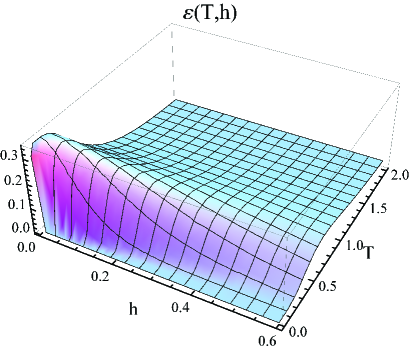
Figure 1: Measure of entanglement production, under ferromagnetic coupling ($J>0$), as a function of dimensionless variables $T$ and $h$.

7.3 Entanglement production under antiferromagnetic coupling ($J<0$)

Under antiferromagnetic coupling of qubits, the measure of entanglement production behaves in a different way, depending on whether $h<1$, $h=1$, or $h>1$.

At low temperature and $h$ in the interval $0\leq h<1$ the asymptotic behavior of the measure is

$$\varepsilon(T,h)\simeq\frac{1}{2}\;\ln 2\;-\;\frac{1}{2}\;e^{-(1-h)/T}\qquad(T\rightarrow 0\;,\;\;0\leq h<1)\;,$$ (7.36)

so that

$$\lim_{T\rightarrow 0}\varepsilon(T,h)=\frac{1}{2}\;\ln 2\qquad(0\leq h<1)\;.$$ (7.37)

But, if $h=1$ and $T\rightarrow 0$, then

$$\varepsilon(T,h)\simeq\frac{1}{2}\;\ln\;\frac{27}{25}\;-\;\frac{1}{15}\;e^{-2/T}\;-\;\frac{2}{225}\;e^{-4/T}\qquad(T\rightarrow 0\;,\;\;h\equiv 1)\;,$$ (7.38)

which gives

$$\lim_{T\rightarrow 0}\varepsilon(T,h)=\frac{1}{2}\;\ln\;\frac{27}{25}\qquad(h\equiv 1)\;.$$ (7.39)

And, if $h>1$, the limit of low temperatures becomes

$$\lim_{T\rightarrow 0}\varepsilon(T,h)=0\qquad(h>1)\;.$$ (7.40)

For small $h$, but finite temperature, we have

$$\varepsilon(T,h)\simeq c_{0}+c_{2}h^{2}\qquad(h\rightarrow 0\;,\;\;T>0)\;,$$ (7.41)

with the coefficients

$$c_{0}=\frac{1}{2}\;\ln\;\frac{2\cosh(1/T)}{1+\cosh(1/T)}\;,\qquad c_{2}=\frac{(e^{1/T}-1)(1-2e^{1/T}-2e^{2/T})}{2T^{2}(e^{1/T}+1)^{2}(e^{2/T}+1)}\;.$$ (7.42)

At high temperature, but finite $h$, we find

$$\varepsilon(T,h)\simeq\frac{1}{8}\left(e^{1/T}-1\right)^{2}\;-\;\frac{h^{2}+1}{8}\;\left(e^{1/T}-1\right)^{3}\qquad(T\rightarrow\infty\;,\;\;h\geq 0)\;,$$ (7.43)

hence

$$\lim_{T\rightarrow\infty}\varepsilon(T,h)=0\qquad(h\geq 0)\;.$$ (7.44)

And when $h\rightarrow\infty$, at finite temperature, we obtain

$$\varepsilon(T,h)\simeq b_{2}e^{-2h/T}+b_{3}e^{-3h/T}\qquad(h\rightarrow\infty\;,\;\;T\geq 0)\;,$$ (7.45)

with the same coefficients $b_{2}$ and $b_{3}$ as in the high-field limit (7.32). Therefore

$$\lim_{h\rightarrow\infty}\varepsilon(T,h)=0\qquad(T\geq 0)\;.$$ (7.46)

Figure 2 shows the general behavior of the entanglement production measure, under antiferromagnetic coupling, as a function of the dimensionless variables $T$ and $h$. The maximal value (7.37) is reached at low temperature and $h<1$.

Figure 2: Measure of entanglement production, under antiferromagnetic coupling ($J<0$), as a function of dimensionless variables $T$ and $h$.

8 Hilbert space partitioning

For many systems, as studied in the previous sections, the partitioning of the Hilbert space has been uniquely fixed. For more complex systems, the type of partitioning may be not unique. Respectively, the entangling properties of the system statistical operator depend on which parts of the system are being entangled. To illustrate how different kinds of partitioning could arise, let us consider a system of $N$ particles with spins. For brevity, we can combine the spatial, $r_{i}$, and spin, $\sigma_{i}$, degrees of freedom in the notation $x_{i}=\{r_{i},\sigma_{i}\}$. The system wave function $|\Psi_{nl}\rangle$ depends on the multi-indices $n$ and $l$ for the spatial and spin states, respectively. The function

$$|\Psi_{nl}\rangle=[\Psi_{nl}(x_{1},x_{2},\ldots,x_{N})]$$ (8.1)

can be treated as a column with respect to all its variables, so that its normalization reads as

$$\langle\Psi_{nl}|\Psi_{nl}\rangle=\int|\Psi_{nl}(x_{1},x_{2},\ldots,x_{N})|^{2}\;dx_{1}\ldots dx_{N}=1\;.$$ (8.2)

As usual, summation with respect to discrete indices is assumed. The system statistical operator

$$\hat{\rho}_{nl}=|\Psi_{nl}\rangle\langle\Psi_{nl}|$$ (8.3)

acts on the Hilbert space $\mathcal{H}$.

8.1 Particle partitioning

The natural partitioning of the system Hilbert space is with respect to particles composing the system. Then we can define the real-space single-particle Hilbert space

$${\cal H}_{i}^{spat}={\rm span}\{\varphi_{n_{i}}({\bf r}_{i})\}$$ (8.4)

as a closed linear envelope over a single-particle basis depending on real-space coordinates. Similarly, a spin-dependent basis defines the Hilbert space

$${\cal H}_{i}^{spin}={\rm span}\{|\sigma_{i}\rangle\}\;.$$ (8.5)

Then a single-particle Hilbert space is

$${\cal H}_{i}={\cal H}_{i}^{spat}\bigotimes{\cal H}_{i}^{spin}\;.$$ (8.6)

The total system Hilbert space can be represented as a tensor product

$${\cal H}=\bigotimes_{i=1}^{N}{\cal H}_{i}$$ (8.7)

of single-particle spaces.

Following the general scheme, we define the reduced statistical operators

$$\hat{\rho}_{nl}^{(i)}\equiv{\rm Tr}_{{\cal H}/{\cal H}_{i}}\hat{\rho}_{nl}\;,$$ (8.8)

whose tensor product induces the nonentangling operator

$$\hat{\rho}_{nl}^{\otimes}=\bigotimes_{i=1}^{N}\hat{\rho}_{nl}^{(i)}\;.$$ (8.9)

Then the entanglement production of the statistical operator (8.3), with respect to the Hilbert space partitioning (8.7), is quantified by the measure

$$\varepsilon(\hat{\rho}_{nl})\equiv\log\;\frac{||\hat{\rho}_{nl}||}{||\hat{\rho}_{nl}^{\otimes}||}=-\log||\hat{\rho}_{nl}^{\otimes}||\;.$$ (8.10)

Keeping in mind indistinguishable particles, we get

$$||\hat{\rho}_{nl}^{\otimes}||=\prod_{i=1}^{N}||\hat{\rho}_{nl}^{(i)}||=||\hat{\rho}_{nl}^{(i)}||^{N}\;.$$ (8.11)

Therefore measure (8.10) becomes

$$\varepsilon(\hat{\rho}_{nl})=-\;\frac{N}{2}\;\log\left({\rm Tr}_{{\cal H}_{i}}(\hat{\rho}_{nl}^{(i)})^{2}\right)\;.$$ (8.12)

Note that we have no problems dealing with indistinguishable particles, while the definition of state entanglement for indistinguishable particles confronts some problems [91, 92]. All we need is to correctly symmetrize the system wave function depending on whether bosons or fermions are considered.

8.2 Spin-spatial partitioning

It is also interesting to study the entanglement between spin and spatial degrees of freedom [93, 94, 95, 96, 97]. To consider such a spin-spatial entanglement production, it is necessary to partition the system Hilbert space onto spin and spatial degrees of freedom. For this purpose, we introduce the real-space Hilbert part

$${\cal H}_{spat}\equiv\bigotimes_{i=1}^{N}{\cal H}_{i}^{spat}$$ (8.13)

and the spin Hilbert space

$${\cal H}_{spin}\equiv\bigotimes_{i=1}^{N}{\cal H}_{i}^{spin}\;.$$ (8.14)

Then the total Hilbert space is a tensor product of the spatial and spin parts

$${\cal H}={\cal H}_{spat}\bigotimes{\cal H}_{spin}\;.$$ (8.15)

The related reduced operators are

$$\hat{\rho}_{nl}^{spat}={\rm Tr}_{{\cal H}_{spin}}\hat{\rho}_{nl}\;,\qquad\hat{\rho}_{nl}^{spin}={\rm Tr}_{{\cal H}_{spat}}\hat{\rho}_{nl}\;,$$ (8.16)

defining the non-entangling operator

$$\hat{\rho}_{nl}^{\otimes}=\hat{\rho}_{nl}^{spat}\bigotimes\hat{\rho}_{nl}^{spin}\;.$$ (8.17)

This gives the entanglement production measure for the system statistical operator, with respect to the entanglement of spin and spatial degrees of freedom, as

$$\overline{\varepsilon}(\hat{\rho}_{nl})\equiv\log\;\frac{||\hat{\rho}_{nl}||}{||\hat{\rho}_{nl}^{\otimes}||}=-\log\left(||\hat{\rho}_{nl}^{spat}||\cdot||\hat{\rho}_{nl}^{spin}||\right)\;.$$ (8.18)

Employing the Hilbert-Schmidt norm yields

$$\overline{\varepsilon}(\hat{\rho}_{nl})=-\frac{1}{2}\left[\log\;{\rm Tr}_{{\cal H}_{spat}}\left(\hat{\rho}_{nl}^{spat}\right)^{2}+\log\;{\rm Tr}_{{\cal H}_{spin}}\left(\hat{\rho}_{nl}^{spin}\right)^{2}\right]\;.$$ (8.19)

Quantities (8.12) and (8.19) are different. In the following section, we present explicit calculation of their values.

9 Multiparticle spinor quantum system

9.1 Permutation-invariant wavefunctions of spinor particles

This section formulates general properties of many-body wavefunctions of indistinguishable spinor particles with separable spin and spatial degrees of freedom. Such a system is described by the Hamiltonian $\hat{H}_{\mathrm{spat}}+\hat{H}_{\mathrm{spin}}$, where $\hat{H}_{\mathrm{spat}}$ is spin-independent, $\hat{H}_{\mathrm{spin}}$ is spatially-homogeneous, and each of $\hat{H}_{\mathrm{spat}}$ and $\hat{H}_{\mathrm{spin}}$ is permutation-invariant. The wavefunctions are composed from the spin $\Xi_{tl}^{[\lambda]}$ and spatial $\Phi_{tn}^{[\lambda]}$ functions, which form bases of irreducible representations of the symmetric group $\mathcal{S}_{N}$ of $N$-symbol permutations (see [39, 40, 41, 54, 98]). This means that a permutation $\mathcal{P}$ of the particles transforms each basis function to a linear combination of the functions in the same representation,

$$\mathcal{P}\Xi_{tl}^{[\lambda]} =\sum_{t^{\prime}}D_{t^{\prime}t}^{[\lambda]}(\mathcal{P})\Xi_{t^{\prime}l}^{[\lambda]}\;,$$ (9.1)

$$\mathcal{P}\Phi_{tn}^{[\lambda]} =\mathrm{sgn}(\mathcal{P})\sum_{t^{\prime}}D_{t^{\prime}t}^{[\lambda]}(\mathcal{P})\Phi_{t^{\prime}n}^{[\lambda]}\;.$$ (9.2)

Here, the irreducible representations are associated with the Young diagram $\lambda=[\lambda_{1},\ldots,\lambda_{M}]$. The number of the diagram rows $M=2s+1$ is the multiplicity, where $s$ is the particle’s spin. The basic functions of the representation are labeled by the standard Young tableaux $t$ of the shape $\lambda$. The factor $\mathrm{sgn}(\mathcal{P})$ is the permutation parity for fermions and $\mathrm{sgn}(\mathcal{P})\equiv 1$ for bosons. The Young orthogonal representation matrices $D_{t^{\prime}t}^{[\lambda]}(\mathcal{P})$ satisfy the following relations,

$$D_{tt^{\prime}}^{[\lambda]}(\mathcal{P}) =D_{t^{\prime}t}^{[\lambda]}(\mathcal{P}^{-1})\;,$$ (9.3)

$$\sum_{t^{\prime}}D_{rt^{\prime}}^{[\lambda]}(\mathcal{P})D_{t^{\prime}t}^{[\lambda]}(\mathcal{Q}) =D_{rt}^{[\lambda]}(\mathcal{P}\mathcal{Q})\;,$$ (9.4)

$$\sum_{\mathcal{P}}D_{t^{\prime}r^{\prime}}^{[\lambda^{\prime}]}(\mathcal{P})D_{tr}^{[\lambda]}(\mathcal{P}) =\frac{N!}{f_{\lambda}}\delta_{\lambda\lambda^{\prime}}\delta_{tt^{\prime}}\delta_{rr^{\prime}}\;,$$ (9.5)

$$D_{t^{\prime}t}^{[\lambda]}(\mathcal{E}) =\delta_{t^{\prime}t}\;,$$ (9.6)

where $\mathcal{E}$ is the identity permutation. These relations provide the proper bosonic or fermionic permutation symmetry of the total wavefunction

$$\Psi_{nl}^{[\lambda]}=f_{\lambda}^{-1/2}\sum_{t}\Phi_{tn}^{[\lambda]}\Xi_{tl}^{[\lambda]}\;,$$ (9.7)

$\mathcal{P}\Psi^{[\lambda]}_{nl}=\mathrm{sgn}(\mathcal{P})\Psi^{[\lambda]}_{nl}$. The representation dimension is given by

$$f_{\lambda}=\frac{N!\prod_{m<m^{\prime}}(\lambda_{m}-m-\lambda_{m^{\prime}}+m^{\prime})}{\prod_{m=1}^{M}(\lambda_{m}+M-m)!}\;.$$ (9.8)

For spin-$1/2$ particles, the Young diagrams have two rows and are unambiguously related to the total spin $S$, $\lambda=[N/2+S,N/2-S]$. The representation dimension can be expressed as

$$f_{\lambda}=\frac{N!(2S+1)}{(N/2+S+1)!(N/2-S)!}\;.$$ (9.9)

An explicit expression for the spin wavefunction is obtained [99] in the case of commutative $\hat{H}_{\mathrm{spin}}$ and the total spin projection operator $\hat{S}_{z}$,

$$\Xi_{tS_{z}}^{[\lambda]}=C_{SS_{z}}\sum_{\mathcal{P}}D_{t[0]}^{[\lambda]}(\mathcal{P})\prod_{j=1}^{N/2+S_{z}}|\uparrow(\mathcal{P}j)\rangle\prod_{j=N/2+S_{z}+1}^{N}|\downarrow(\mathcal{P}j)\rangle\;.$$ (9.10)

The wavefunction is unambiguously determined by the total spin $S$ and its projection $S_{z}$, which is the half of the difference of the occupations of the two spin states $|\uparrow\rangle$ and $|\downarrow\rangle$. The normalization factor is expressed as [99]

$$C_{SS_{z}}=\frac{1}{(N/2+S_{z})!(N/2-S)!}\sqrt{\frac{(2S+1)(S+S_{z})!}{(N/2+S+1)(2S)!(S-S_{z})!}}\;.$$ (9.11)

9.2 Spin-spatial partitioning

The spin-spatial entanglement production measure can be evaluated for a generic system of indistinguishable spinor particles with separable spin and spatial degrees of freedom. Due to the orthogonality of the spin and spatial functions, $\left\langle\Xi_{t^{\prime}l}^{[\lambda]}|\Xi_{tl}^{[\lambda]}\right\rangle=\delta_{tt^{\prime}}$, $\left\langle\Phi_{tn}^{[\lambda]}|\Phi_{t^{\prime}n}^{[\lambda]}\right\rangle=\delta_{tt^{\prime}}$, we have for the total wavefunction (9.7)

$$\hat{\rho}^{\mathrm{spin}}_{nl}={\rm Tr}_{{\cal H}_{spat}}\left|\Psi_{nl}^{[\lambda]}\right\rangle\left\langle\Psi_{nl}^{[\lambda]}\right|=\frac{1}{f_{\lambda}}\sum_{t,t^{\prime}}\left\langle\Phi_{tn}^{[\lambda]}|\Phi_{t^{\prime}n}^{[\lambda]}\right\rangle\left|\Xi_{tl}^{[\lambda]}\right\rangle\left\langle\Xi_{t^{\prime}l}^{[\lambda]}\right|=\frac{1}{f_{\lambda}}\sum_{t}\left|\Xi_{tl}^{[\lambda]}\right\rangle\left\langle\Xi_{tl}^{[\lambda]}\right|$$ (9.12)

and, similarly,

$$\hat{\rho}^{\mathrm{spat}}_{nl}=\frac{1}{f_{\lambda}}\sum_{t}\left|\Phi_{tn}^{[\lambda]}\right\rangle\left\langle\Phi_{tn}^{[\lambda]}\right|\;.$$ (9.13)

Then

$${\rm Tr}_{{\cal H}_{spat}}\left(\hat{\rho}^{\mathrm{spat}}_{nl}\right)^{2}=\frac{1}{f_{\lambda}^{2}}\sum_{t,t^{\prime}}\left\langle\Phi_{tn}^{[\lambda]}|\Phi_{t^{\prime}n}^{[\lambda]}\right\rangle\left\langle\Phi_{t^{\prime}n}^{[\lambda]}|\Phi_{tn}^{[\lambda]}\right\rangle=\frac{1}{f_{\lambda}^{2}}\sum_{t,t^{\prime}}\delta_{tt^{\prime}}^{2}=\frac{1}{f_{\lambda}}$$ (9.14)

and

$${\rm Tr}_{{\cal H}_{spin}}\left(\hat{\rho}^{\mathrm{spin}}_{nl}\right)^{2}=\frac{1}{f_{\lambda}}\;.$$ (9.15)

Therefore, according to Eq. (8.19), the entanglement production measure

$$\overline{\varepsilon}(\hat{\rho}_{nl})=\ln f_{\lambda}$$ (9.16)

depends only on the representation dimension (9.8).

The leading term of the asymptotic expansion in the limit $N\rightarrow\infty$ can be evaluated using the Stirling formula in Eq. (9.8) as

$$\overline{\varepsilon}(\hat{\rho}_{nl})\sim N\ln N-\sum_{m=1}^{N}\lambda_{m}\ln\lambda_{m}\;.$$ (9.17)

Its maximum, $\overline{\varepsilon}(\hat{\rho}_{nl})=N\ln M$, is attained for equal lengths of the Young diagram rows $\lambda_{m}=N/M$.

For spin-$1/2$ particles, the entanglement production measure decreases when $S$ increases (see Fig. 3). The measure vanishes at $S=N/2$, when the total wavefunction is a single product of the spin and spatial functions. The plot for $N\to\infty$ is obtained using the leading term in the asymptotic expansion,

$$\overline{\varepsilon}(\hat{\rho}_{nl})\sim-N\left[\left(\frac{1}{2}-\frac{S}{N}\right)\ln\left(\frac{1}{2}-\frac{S}{N}\right)+\left(\frac{1}{2}+\frac{S}{N}\right)\ln\left(\frac{1}{2}+\frac{S}{N}\right)\right]\;.$$ (9.18)

In the asymptotic limit, the entanglement production measure attains its maximum of $\overline{\varepsilon}(\hat{\rho}_{nl})=N\ln 2$ at $S=0$, when the Young diagram rows have the equal length.

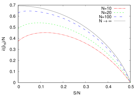
Figure 3: The spin-spatial entanglement production measure for the statistical operator of $N$ spin-$\frac{1}{2}$ particles in the state with the defined spin $S$. The red dot-dashed, green short-dashed, and blue long-dashed lines correspond to $N=10$, $20$, and $100$, respectively. The limiting case of $N\to\infty$ is shown by the black solid line.

9.3 Particle partitioning

The particle entanglement production measure can be evaluated in the particular case of non-interacting particles with $s=\frac{1}{2}$. If there are several spatial orbitals $|0\rangle,\ldots|M-1\rangle$, there are multiple spatial wavefunctions for the given $\lambda$ and the orbital occupations, even if $\hat{H}_{\mathrm{spat}}$ commutes with the orbital occupations (see [40, 54, 98]). However, if there are only two spatial orbitals, $|+\rangle$ and $|-\rangle$, and $\hat{H}_{\mathrm{spat}}$ commutes with the “isotopic spin” $\hat{I}_{z}=\sum_{j=1}^{N}(|+(j)\rangle\langle+(j)|-|-(j)\rangle\langle-(j)|)/2$, the spatial wavefunction is unambiguously determined by the total spin $S$ and the eigenvalue $I_{z}$ of $\hat{I}_{z}$ (it is nothing but the half of the difference of the orbital occupations) and can be represented for bosons like (9.10),

$$\Phi_{tI_{z}}^{[\lambda]}=C_{SI_{z}}\sum_{\mathcal{P}}D_{t[0]}^{[\lambda]}(\mathcal{P})\prod_{j=1}^{N/2+I_{z}}|+(\mathcal{P}j)\rangle\prod_{j=N/2+I_{z}+1}^{N}|-(\mathcal{P}j)\rangle\;.$$ (9.19)

Here the normalization factor is defined by Eq. (9.11). Given $S$, the system state is specified by two independent spin projections, $S_{z}$, and $I_{z}$. Then the multi-indices $n$ and $l$ can be specifically chosen as $I_{z}$ and $S_{z}$. Ground states of such systems were analyzed in Refs. [100, 101] using $SU(2)$ symmetry ($SU(2)$ and symmetric groups are closely related, having a common set of basic functions of irreducible representations, see [40]).

In the particular basic, the reduced statistical operators (8.8) have the following explicit form,

$$\hat{\rho}^{(i)}_{I_{z}S_{z}}=\sum_{\{n\},\{\sigma\}}\prod_{i^{\prime}\neq i}\langle n(i^{\prime})|\langle\sigma(i^{\prime})|\Psi_{I_{z}S_{z}}^{[\lambda]}\rangle\langle\Psi_{I_{z}S_{z}}^{[\lambda]}|\prod_{i^{\prime\prime}\neq i}|n(i^{\prime\prime})\rangle|\sigma(i^{\prime\prime})\rangle\;,$$ (9.20)

where $n$ can be $+$ or $-$, $\sigma$ can be $\uparrow$ or $\downarrow$, and the summation is performed over all $n_{i^{\prime}}$ and $\sigma_{i^{\prime}}$ with $i^{\prime}\neq i$. Their matrix elements can be expressed as matrix elements of the projection operator

$$\langle n^{\prime},\sigma^{\prime}|\hat{\rho}^{(i)}_{I_{z}S_{z}}|n,\sigma\rangle=\langle\Psi_{I_{z}S_{z}}^{[\lambda]}|n(i)\rangle|\sigma(i)\rangle\langle n(i)|\langle\sigma(i)|\Psi_{I_{z}S_{z}}^{[\lambda]}\rangle\delta_{nn^{\prime}}\delta_{\sigma\sigma^{\prime}}\>.$$ (9.21)

Due to permutation symmetry of the total wavefunction, the matrix element

$$\langle n,\sigma|\hat{\rho}^{(i)}_{I_{z}S_{z}}|n,\sigma\rangle=\langle\Psi_{I_{z}S_{z}}^{[\lambda]}|\hat{P}_{n\sigma}|\Psi_{I_{z}S_{z}}^{[\lambda]}\rangle$$ (9.22)

is independent of $i$. Here

$$\hat{P}_{n\sigma}\equiv\frac{1}{N}\sum_{i=1}^{N}|n(i)\rangle|\sigma(i)\rangle\langle n(i)|\langle\sigma(i)|=$$

$$=\frac{1}{4}+\frac{\delta_{\sigma\uparrow}-\delta_{\sigma\downarrow}}{2N}\hat{S}_{z}+\frac{\delta_{n+}-\delta_{n-}}{2N}\hat{I}_{z}+\frac{(\delta_{\sigma\uparrow}-\delta_{\sigma\downarrow})(\delta_{n+}-\delta_{n-})}{N}\sum_{i=1}^{N}\hat{s}_{z}(i)\hat{i}_{z}(i)$$ (9.23)

is represented in terms of the spin $\hat{s}_{z}(i)=\frac{1}{2}(|\uparrow(i)\rangle\langle\uparrow(i)|-|\downarrow(i)\rangle\langle\downarrow(i)|)$ and isotopic spin $\hat{i}_{z}(i)=\frac{1}{2}(|+(i)\rangle\langle+(i)|-|-(i)\rangle\langle-(i)|)$ of the $i$th particle. The operator $\sum_{i=1}^{N}\hat{s}_{z}(i)\hat{i}_{z}(i)$, as an operator in the spin space, is a component of an irreducible spherical vector (see [98]). Then its matrix elements between states with arbitrary $S_{z}$ can be related to ones for $S_{z}=S$ using the Wigner-Eckart theorem (see [98]). In the case of two spacial orbitals, the same can be done for $I_{z}$ too, providing

$$\langle\Psi_{I_{z}S_{z}}^{[\lambda]}|\sum_{i=1}^{N}\hat{s}_{z}(i)\hat{i}_{z}(i)|\Psi_{I_{z}S_{z}}^{[\lambda]}\rangle=\frac{I_{z}S_{z}}{S^{2}}\langle\Psi_{SS}^{[\lambda]}|\sum_{i=1}^{N}\hat{s}_{z}(i)\hat{i}_{z}(i)|\Psi_{SS}^{[\lambda]}\rangle\;.$$ (9.24)

Since $\Psi_{I_{z}S_{z}}^{[\lambda]}$ is an eigenfunction of $\hat{S}_{z}$ and $\hat{I}_{z}$, the matrix element of the reduced statistical operators can be related to the one for $S_{z}=I_{z}=S$,

$$\langle n,\sigma|\hat{\rho}^{(i)}_{I_{z}S_{z}}|n,\sigma\rangle=\frac{1}{4}\left(1-\frac{I_{z}S_{z}}{S^{2}}\right)+\frac{\delta_{n+}-\delta_{n-}}{2N}I_{z}\left(1-\frac{S_{z}}{S}\right)+$$

$$+\frac{\delta_{\sigma\uparrow}-\delta_{\sigma\downarrow}}{2N}S_{z}\left(1-\frac{I_{z}}{S}\right)+\frac{I_{z}S_{z}}{S^{2}}\langle n,\sigma|\hat{\rho}^{(i)}_{SS}|n,\sigma\rangle\;.$$ (9.25)

The latter matrix element can be transformed, using Eqs. (9.7) and (9.21), to the sum of the products

$$\langle n,\sigma|\hat{\rho}^{(i)}_{SS}|n,\sigma\rangle=\frac{1}{f_{\lambda}}\sum_{t,t^{\prime}}\langle\Xi_{tS}^{[\lambda]}|\sigma(i)\rangle\langle\sigma(i)|\Xi_{t^{\prime}S}^{[\lambda]}\rangle\langle\Phi_{tS}^{[\lambda]}|n(i)\rangle\langle n(i)|\Phi_{t^{\prime}S}^{[\lambda]}\rangle$$ (9.26)

of the spin and spatial matrix elements. The spin matrix elements can be represented as

$$\langle\Xi_{tS}^{[\lambda]}|\sigma(i)\rangle\langle\sigma(i)|\Xi_{t^{\prime}S}^{[\lambda]}\rangle=[\delta_{\sigma\downarrow}\delta_{tt^{\prime}}+(\delta_{\sigma\uparrow}-\delta_{\sigma\downarrow})\langle\Xi_{t^{\prime}S}^{[\lambda]}|\uparrow(i)\rangle\langle\uparrow(i)|\Xi_{tS}^{[\lambda]}\rangle]\;,$$ (9.27)

where

$$\langle\Xi_{t^{\prime}S}^{[\lambda]}|\uparrow(i)\rangle\langle\uparrow(i)|\Xi_{tS}^{[\lambda]}\rangle=(\lambda_{1}-1)!\lambda_{2}!\lambda_{1}^{2}C_{SS}^{2}\sum_{\mathcal{Q}}D_{t[0]}^{[\lambda]}(\mathcal{Q})D_{t^{\prime}[0]}^{[\lambda]}(\mathcal{Q})\delta_{i\mathcal{Q}\lambda_{1}}$$ (9.28)

was calculated in Ref. [98].

Using similar expressions for the spatial matrix elements, Eqs. (9.3), (9.4), and (9.6), one gets

$$\langle n,\sigma|\hat{\rho}^{(i)}_{SS}|n,\sigma\rangle=\delta_{\sigma\downarrow}\delta_{n-}+$$

$$+(\delta_{\sigma\uparrow}\delta_{n-}+\delta_{\sigma\downarrow}\delta_{n+}-2\delta_{\sigma\downarrow}\delta_{n-})\frac{\lambda_{1}}{N}+(\delta_{\sigma\uparrow}-\delta_{\sigma\downarrow})(\delta_{n+}-\delta_{n-})\left(\frac{\lambda_{1}}{N!}\right)^{2}f_{\lambda}\varSigma_{jj}^{(S,S)}\;,$$ (9.29)

where

$$\varSigma_{jj}^{(S,S)}=\frac{N!(N-1)!}{f_{S}\lambda_{1}^{2}}\left[\lambda_{1}-\frac{\lambda_{2}}{\lambda_{1}-\lambda_{2}+2}\right]$$ (9.30)

was calculated in [98].

Then Eqs. (8.12) and (9.25) provide the particle entanglement production measure

$$\varepsilon(\hat{\rho}_{I_{z}S_{z}})=-\frac{N}{2}\ln\left(\frac{1}{4}+\frac{1}{N^{2}}\left[S_{z}^{2}+I_{z}^{2}+\frac{(N+2)^{2}}{4S^{2}(S+1)^{2}}S_{z}^{2}I_{z}^{2}\right]\right)\;.$$ (9.31)

Its maximal value $N\ln 2$ is attained at $S_{z}=I_{z}=0$ for any $S$ and $N$ (see Figs. 4 and 5). In the case of the spin-spatial partition, this value can be reached only in the limit $N\to\infty$. The particle and spin-spatial entanglement production measures both vanish at $S_{z}=I_{z}=S=N/2$. However, given $0<S_{z}<N/2$ or $0<I_{z}<N/2$, the particle entanglement increases with $S$, being maximal at $S=N/2$, when the total wavefunction is a single product of the spin and spatial functions and the spin-spatial entanglement vanishes.

Figure 4: The particle entanglement production measure for the statistical operator of $N=10$ spin-$\frac{1}{2}$ particles in the state with the defined spin $S$, calculated with Eq. (9.31). The red dot-dashed, blue dashed, and black solid lines correspond to $I_{z}=0$, $I_{z}=S_{z}$, and $I_{z}=S$, respectively.

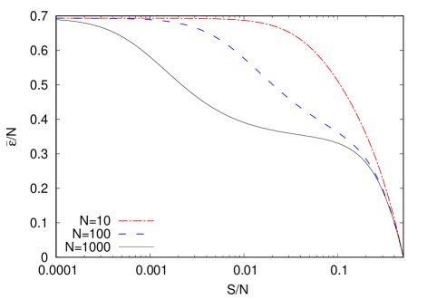
Figure 5: The particle entanglement production measure for the statistical operator of $N$ spin-$\frac{1}{2}$ particles in the state with $I_{z}=S_{z}=S$. The red dot-dashed, blue dashed, and black solid lines are calculated with Eq. (9.31) for $N=10$, $100$, and $1000$, respectively.

10 Conclusion

Dealing with statistical operators, one can consider two different notions. One is the state entanglement characterizing the structure of the given statistical operator. The other notion is the entanglement production by the statistical operator, describing the action of the statistical operator on the given Hilbert space and showing how this action creates entangled functions from disentangled ones. These two notions are principally different and should not be confused.

The operational meaning of the entangling power of statistical operators is the same as for any other operator defined on a Hilbert space: it shows the ability of an operator to produce entangled wave functions of the given Hilbert space. Throughout the paper, the notion of entanglement production has been used in line the commonly accepted in mathematical literature [16, 17, 18, 19, 20, 21, 22, 23, 26].

Entangling properties of statistical operators play an important role in several branches of quantum theory, such as quantum measurements, quantum information processing, quantum computing, and quantum decision theory, where one deals with composite measurements and composite events, related to composite probability measures. Entangling properties of statistical operators influence the structure of probability measures they generate. Depending on whether the statistical operator is entangling or not, the resulting probability measure can be either not factorizable or factorizable, as is discussed in Sec. 2.

We have defined the measure of entanglement production by statistical operators and illustrated it by several examples of entangled pure states, equilibrium Gibbs states, and by the case of a multiparticle spinor system. The relation of the introduced measure to other known concepts, such as quantum state purity, linear entropy or impurity, inverse participation ratio, quadratic Rényi entropy, and correlators in composite measurements, is thoroughly discussed. The measure can be defined for a collection of quantum systems or for a set of operators characterizing a quantum system after measurements. The phenomenon of decoherence is also shown to be intimately related to entanglement production.

For complex spinor systems, the measure of entanglement production depends on the type of partitioning of the total Hilbert space. Thus, it is possible to realize particle partitioning or spin-spatial partitioning. Both these cases are analyzed. The analysis demonstrates when the entanglement production is maximal and when it tends to zero, which can be used in the applications of quantum theory mentioned above.

References

- [1] Williams C P and Clearwater S H 1998 Explorations in Quantum Computing ( New York: Springer)
- [2] Nielsen M A and Chuang I L 2000 Quantum Computation and Quantum Information (New York: Cambridge University Press)
- [3] Vedral V 2002 Rev. Mod. Phys. 74 197–234
- [4] Keyl M 2002 Phys. Rep. 369 431–548
- [5] Horodecki R, Horodecki P, Horodecki M and Horodecki K 2009 Rev. Mod. Phys. 81 865–942
- [6] Gühne O and Toth G 2009 Phys. Rep. 474 1–75
- [7] Wilde M 2013 Quantum Information Theory (Cambridge: Cambridge University Press)
- [8] Eltschka C and Siewert J 2014 J. Phys. A: 47 424005
- [9] Yukalov V I and Sornette D 2016 Phil. Trans. Roy. Soc. A 374 20150100
- [10] Zanardi P 2001 Phys. Rev. A 63 040304
- [11] Balakrishnan S and Sankaranarayanan R 2009 Phys. Rev. A 79 052339
- [12] Macchiavello C and Rossi M 2013 J. Phys. Conf. Ser. 470 012005
- [13] Yukalov V I and Sornette D 2013 Laser Phys. 23 105502
- [14] Kong F Z, Zhao J L, Yang M and Cao Z L 2015 Phys. Rev. A 92 012127
- [15] Zanardi P, Zalka C and Faoro L 2000 Phys. Rev. A 62 030301
- [16] Marcus M and Moyls B N 1959 Pacif. J. Math. 9 1215–1221
- [17] Westwick R 1967 Pacif. J. Math. 23 613–620
- [18] Johnston N 2011 Lin. Multilin. Algebra 59 1171–1187
- [19] Beasley L 1988 Lin. Algebra Appl. 107 161–167
- [20] Alfsen E and Shultz F 2010 J. Math. Phys. 51 052201
- [21] Friedland S, Li C K, Poon Y T, and Sze N S 2011 J. Math. Phys. 52, 042203
- [22] Gohberg J and Goldberg S 1987 J. Math. Anal. Appl. 125 124–140
- [23] Crouzeux J P and Hassouni A 1994 SIAM J. Optimiz. 4 649–658
- [24] Fan H Y 2001 Mod. Phys. Lett. B 15 1475–1483
- [25] Dao–Ming L 2016 Int. J. Theor. Phys. 55 3156–3163
- [26] Chen J, Duan R, Ji Z, Ying M and Yu J 2008 J. Math. Phys. 49 012103
- [27] Yukalov V I 2003 Phys. Rev. Lett. 90 167905
- [28] Yukalov V I 2003 Phys. Rev. A 68 022109
- [29] Rudin W 1991 Functional Analysis (New York: McGraw-Hill)
- [30] Conway J B 2000 A Course in Operator Theory (Providence: AMS Press)
- [31] Yukalov V I 2003 Mod. Phys. Lett. B 17 95–103
- [32] Yukalov V I and Yukalova E P 2006 Laser Phys. 16 354–359
- [33] Yukalov V I and Yukalova E P 2006 Phys. Rev. A 73 022335
- [34] Yukalov V I 2004 Laser Phys. 14 1403–1414
- [35] Yukalov V I and Yukalova E P 2015 Phys. Rev. A 92 052121
- [36] Birman J L, Nazmitdinov R G and Yukalov V I 2013 Phys. Rep. 526 1–91
- [37] Kubo R 1968 Thermodynamics (Amsterdam: North Holland)
- [38] Kaplan I 2013 Found. Phys. 43 1233–1251
- [39] Hamermesh M 1989 Group Theory and Its Application to Physical Problems (Mineola: Dover)
- [40] Kaplan I G 1975 Symmetry of Many-Electron Systems ( London: Academic Press)
- [41] Pauncz R 1995 The Symmetric Group in Quantum Chemistry (Boca Raton: CRC Press)
- [42] Wigner E 1927 Z. Phys. 40 883–892
- [43] Heitler W 1927 Z. Phys. 46 47–72
- [44] Dirac P A M 1929 Proc. R. Soc. A 123 714–733
- [45] Lieb E and Mattis D 1962 Phys. Rev. 125 164–172
- [46] Yang C N 1967 Phys. Rev. Lett. 19 1312–1315
- [47] Sutherland B 1968 Phys. Rev. Lett. 20 98–100
- [48] Guan L, Chen S, Wang Y and Ma Z Q 2009 Phys. Rev. Lett. 102 160402
- [49] Yang C N 2009 Chin. Phys. Lett. 26 120504
- [50] Gorshkov A V, Hermele M, Gurarie V, Xu C, Julienne P S, Ye J, Zoller P, Demler E, Lukin M D and Rey A M 2010 Nature Phys. 6 289–295
- [51] Fang B, VignoloP, Gattobigio M, Miniatura C, and Minguzzi A 2011 Phys. Rev. A 84 023626
- [52] Daily K M, Rakshit D and Blume D 2012 Phys. Rev. Lett. 109 030401
- [53] Harshman N L 2014 Phys. Rev. A 89 033633
- [54] Yurovsky V A 2014 Phys. Rev. Lett. 113 200406
- [55] Harshman N 2016 Few-Body Syst. 57 11–43
- [56] Harshman N 2016 Few-Body Syst. 57 45–69
- [57] Yurovsky V A 2016 Phys. Rev. A 93 023613
- [58] Brechet S D, Reuse F A, Maschke K and Ansermet J P 2016 Phys. Rev. A 94 042505
- [59] Sela E, Fleurov V, and Yurovsky V A 2016 Phys. Rev. A 94 033848
- [60] Yurovsky V A 2017 Phys. Rev. Lett. 118 200403
- [61] von Neumann J 1955 Mathematical Foundations of Quantum Mechanics (Princeton: Princeton University)
- [62] Benioff P A 1972 J. Math. Phys. 13 908–914
- [63] Holevo A S 1973 J. Multivar. Anal. 8 337–394
- [64] Yukalov V I and Sornette D 2008 Phys. Lett. A 372, 6867–6871
- [65] Yukalov V I and Sornette D 2010 Adv. Compl. Syst. 13 659–698
- [66] Chen L and Yu L 2016 Phys. Rev. A 94 022307
- [67] Yukalov V I and Yukalova E P 2017 J. Phys. Conf. Ser. 826 012021
- [68] Dean P and Bell R J 1970 Discuss. Faraday Soc. 50 55–61
- [69] Edwards J T and Thouless D J 1972 J Phys C: Solid State Phys. 5 807–820
- [70] Heller E J 1987 Phys. Rev. A 35 1360–1370
- [71] Yurovsky V A and Olshanii M 2011 Phys. Rev. Lett. 106 025303
- [72] Olshanii M, Jacobs K, Rigol M, Dunjko V, Kennard H and Yurovsky V A 2012 Nature Commun. 3 641
- [73] Cohen D, Yukalov V I and Ziegler K 2016 Phys. Rev. A 93 042101
- [74] Mirbach B and Korsch A J 1998 Ann. Phys. (N.Y.) 265 80–97
- [75] Baumgratz T, Cramer M and Plenio M B 2014 Phys. Rev. Lett. 113 140401
- [76] Müller-Lennert M, Dupuis F, Szehr O, Fehr S and Tomamichel M 2013 J. Math. Phys. 54 122203
- [77] Calixto M and Romera E 2015 J. Stat. Mech. 2015 P06029
- [78] Linke N M, Johri S, Figgatt C, Landsman K A, Matsuura A Y and Monroe C 2018 Phys. Rev. A 98 052334
- [79] Lüders G 1951 Ann. Phys. (Leipzig) 8 322–328
- [80] Zurek W H 2003 Rev. Mod. Phys. 75 715–776
- [81] Braginsky V B and Khalili F Y 1996 Rev. Mod. Phys. 68 1–12
- [82] Yukalov V I 2002 Phys. Rev. E 65 056118
- [83] Yukalov V I 2012 Phys. Lett. A 376 550–554
- [84] Yukalov V I 2012 Ann. Phys. (N.Y.) 327 253–263
- [85] Kittel C 1996 Introduction to Solid State Physics (New York: Wiley)
- [86] Bochner S and Chandrasekharan K 1949 Fourier Transforms (Princeton: Princeton University)
- [87] Kubo R 1965 Statistical Mechanics (Amsterdam: North-Holland)
- [88] Klimontovich Y L 1986 Statistical Physics (Chur: Harwood)
- [89] Bogolubov N N 2015 Quantum Statistical Mechanics (Singapore: World Scientific)
- [90] Bernstein D S and So W 1993 IEEE Trans. Automatic Control 38 1228–1232
- [91] Amico L, Fazio R, Osterloh A and Vedral V 2008 Rev. Mod. Phys. 80 517–576
- [92] Benatti F, Floreanini R and Titimbo K 2014 Open Syst. Inf. Dynam. 21 1440003
- [93] Omar Y, Pauncovic N, Bose S and Vedral V 2002 Phys. Rev. A 65, 062305
- [94] Karlsson E B and Lovesey S W 2002 Phys. Scr. 65 112–118
- [95] Lamata L and León J 2006 Phys. Rev. A 73 052322
- [96] Wang T G, Song S Y and Long G L 2012 Phys. Rev. A 85 062311
- [97] Kastner R E, Jeknić-Dugić J and Jaroszkiewicz G, Eds. 2017 Quantum Structural Studies (Singapore: World Scientific)
- [98] Yurovsky V A 2015 Phys. Rev. A 91 053601
- [99] Yurovsky V A 2013 Int. J. Quantum Chem. 113 1436–1439
- [100] Kuklov A B and Svistunov B V 2002 Phys. Rev. Lett. 89 170403
- [101] Ashhab S and Leggett A J 2003 Phys. Rev. A 68 063612