BS-Nets: An End-to-End Framework For Band Selection of Hyperspectral Image

Abstract

Hyperspectral image (HSI) consists of hundreds of continuous narrow bands with high spectral correlation, which would lead to the so-called Hughes phenomenon and the high computational cost in processing. Band selection has been proven effective in avoiding such problems by removing the redundant bands. However, many of existing band selection methods separately estimate the significance for every single band and cannot fully consider the nonlinear and global interaction between spectral bands. In this paper, by assuming that a complete HSI can be reconstructed from its few informative bands, we propose a general band selection framework, Band Selection Network (termed as BS-Net). The framework consists of a band attention module (BAM), which aims to explicitly model the nonlinear inter-dependencies between spectral bands, and a reconstruction network (RecNet), which is used to restore the original HSI cube from the learned informative bands, resulting in a flexible architecture. The resulting framework is end-to-end trainable, making it easier to train from scratch and to combine with existing networks. We implement two BS-Nets respectively using fully connected networks (BS-Net-FC) and convolutional neural networks (BS-Net-Conv), and compare the results with many existing band selection approaches for three real hyperspectral images, demonstrating that the proposed BS-Nets can accurately select informative band subset with less redundancy and achieve significantly better classification performance with an acceptable time cost.

I Introduction

Hyperspectral images (HSIs) acquired by remote sensors consist of hundreds of narrow bands containing rich spectral and spatial information, which provides an ability to accurately recognize the region of interest. Over the past decade, HSIs have been widely applied in various fields, ranging from agriculture [1] and land management [2] to medical imaging [3] and forensics [4].

As the development of hyperspectral imaging techniques, the spectral resolution has been improved greatly, resulting in difficulty of analyzing. According to the characteristic of hyperspectral imaging, there is a high correlation between adjacent spectral bands [5, 6, 7]. The high-dimensional HSI data not only increases the time complexity and space complexity but leads to the so-called Hughes phenomenon or curse of dimensionality [8]. As a result, redundancy reduction becomes particularly important for HSI processing.

Band Selection (BS) [9, 10, 11], also known as Feature Selection, is an effective redundancy reduction scheme. Its basic idea is to select a significant band subset which includes most information of the original band set. In contrast to the feature extraction methods [12] which reduces dimensionality based on the complex feature transformation, BS keeps main physical property containing in HSIs [5], which makes it easier to explain and apply in practice.

BS methods basically can be classed as supervised and unsupervised methods [13] based on whether the prior knowledge is used. Owing to more robust performance and higher application prospect, unsupervised BS method has attracted a great deal of attention over the last few decades. Unsupervised BS methods can be further divided into three categories: searching-based, clustering-based, and ranking-based methods [14]. The searching-based BS methods treat band selection as a combinational optimization problem and optimize it using a heuristic searching method, such as multi-objective optimization based band selection (MOBS) [5, 15, 16]. However, heuristic searching methods are generally time-consuming. The clustering-based BS methods assume spectral bands are clusterable [17, 13]. Since the similarity between spectral bands is made full consideration, clustering-based methods have achieved great success in recent years, for example, subspace clustering (ISSC) [10, 7] and sparse non-negative matrix factorization clustering (SNMF) [18]. The ranking-based BS methods endeavor to assign a rank or weight for each spectral band by estimating the band significance, e.g., maximum-variance principal component analysis (MVPCA) [19], sparse representation (SpaBS)[20, 21], and geometry-based band selection (OPBS) [22], etc.

Nevertheless, many existing BS methods are basing on the linear transformation of spectral bands, resulting in the lack of consideration of the inherent nonlinear relationship between spectral bands. Furthermore, most of the BS methods commonly view every single spectral band as a separate image or point and evaluate its significance independently. For example, clustering-based BS methods are essentially clustering spectral images with single channel [10, 7, 20]. Therefore, these methods can not take the global spectral interrelationship into account and are difficult to combine with various post-processing, such as classification [23].

In this paper, we treat HSI band selection as a spectral reconstruction task assuming that spectral bands can be sparsely reconstructed using a few informative bands. Unlike the existing BS methods, we aim to take full consideration of the globally nonlinear spectral-spatial relationship and allow to select significant bands from the complete spectral band set, even the 3-D HSI cubes. To this end, we design a band selection network (BS-Net) based on using deep neural networks (DNNs) [24, 25] to explicitly model the nonlinear interdependencies between spectral bands. Although DNNs have been widely used for HSI classification [26, 27, 28] and feature extraction [29, 26, 30], DNN-based band selection has not attracted much attention yet.

The main contributions of this paper are as follows:

1. We proposed an end-to-end band selection framework based on using deep neural networks to learn the nonlinear interdependencies between spectral bands. To the best of our knowledge, this is among the few deep learning based band selection methods.

2. We implemented two different BS-Nets according to the different application scenarios, i.e., spectral-based BS-Net-FC and spectral-spatial-based BS-Net-Conv.

3. We extensively evaluated the proposed BS-Nets framework from aspects of classification performance and quantitative evaluation, showing that BS-Nets can achieve state-of-the-art results.

The rest of the paper is structured as follows. We first define the notations and review the basic concepts of deep learning in Section II. Second, we introduce the proposed BS-Net architecture and its implementation in Section III. Next, in Section IV, we explain the experiments that performed to investigate the performance of the proposed methods, compared with existing BS methods, and discuss their results. Finally, we conclude with a summary and final remarks in Section V.

II Preliminary

II-A Definition and Notations

We denote a 3-D HSI cube consisting of $b$ spectral bands and $N\times M$ pixels as $\boldsymbol{I}\in\mathbb{R}^{N\times M\times b}$. For convenience, we regard $\boldsymbol{I}$ as a set $\boldsymbol{B}=\left\{\boldsymbol{B}_{i}\right\}_{i=1}^{b}$ which contains $b$ band images, where $\boldsymbol{B}_{i}$ indicates $i$-th band image. HSI band selection can thus be formally defined as a function $\psi:\varOmega=\psi\left(\boldsymbol{B}\right)$ that takes all bands as input and produces a band subset with as less as possible reduction of redundant information and satisfied $\varOmega\subseteq\boldsymbol{B}$, $\left|\varOmega\right|=k<b$.

In the following, unless as otherwise specified herein, we uniformly use tensors to represent the inputs, outputs, and intermediate outputs involved in the neural networks. For example, the input of a convolutional layer is denoted as a 4-D tensor $\boldsymbol{x}\in\mathbb{R}^{n\times m\times c}$, where $n\times m$ is the spatial size of the input feature maps, and $c$ is the number of the channels.

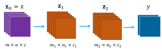
Figure 1: An example of classical CNN with input $\boldsymbol{x}$, output $y$, and two convolutional layers $\boldsymbol{z}_{1}$ and $\boldsymbol{z}_{2}$ .

II-B Convolutional Neural Networks

Deep learning has achieved great success in numerous applications ranging from image recognition to natural language processing [24, 31, 32]. The collection of deep learning methods includes Convolutional Neural Networks (CNN) [25, 33], Generative Adversarial Networks (GAN) [34, 35], and Recurrent Neural Networks (RNN) [36], to name a few. In this section, we take CNN as an example to introduce the basic idea of DNNs, since it is the most popular deep learning method in HSI processing.

Convolutional neural networks (CNN) are inspired by the natural visual perception mechanism of the living creatures [25]. The classical CNN consists of multiple layers of convolutional operations with nonlinear activations, sometimes, followed by a regression layer. A schematic representation of the basic CNN architecture is shown in Fig. 1. We define CNN as a function that takes a tensor $\boldsymbol{x}\in\mathbb{R}^{m\times n\times c}$ as input and produces a certain output $\boldsymbol{y}$. The function can be written as $\boldsymbol{y}=\boldsymbol{f}\left(\boldsymbol{x};\varTheta\right)$, where $\varTheta$ is the trainable parameters consisting of weights and biases involved in CNN.

The training of CNN includes two stages. The first stage is values feedforward wherein each layer yields a dozen of feature maps $\boldsymbol{h}_{i}\in\mathbb{R}^{m_{i}\times n_{i}\times c_{i}}$. Let $\hbar:\mathbb{R}^{m\times n\times c}\rightarrow\mathbb{R}^{m_{i}\times n_{i}\times c_{i}}$ be the convolutional operation and $\boldsymbol{\sigma}$ be a element-wise nonlinear function such as Sigmoid and Rectified Linear Unit (ReLU). The convolutional layer can be represented as

$$\boldsymbol{h}_{i}=\boldsymbol{\sigma}\left(\hbar\left(\boldsymbol{x};\mathbf{W}\right)+\boldsymbol{b}\right)$$ (1)

Here $\mathbf{W}$ and $\boldsymbol{b}$ indicate weights (aka convolutional kernels or convolutional filters) and bias, respectively.

The second stage is called error backpropagation which updates parameters using the gradient descent method. The ultimate goal of CNN is to find an appropriate group of filters to minimize the cost function, e.g., Mean Square Error (MSE) function. The cost function can be denoted as

$$\mathcal{J}\left(\varTheta\right)=Cost\left(\boldsymbol{y},\boldsymbol{f}\left(\boldsymbol{x};\varTheta\right)\right)$$ (2)

The parameters updating is given by

$$\varTheta\eqqcolon\varTheta-\eta\frac{\partial\mathcal{J}}{\partial\varTheta}$$ (3)

Where $\eta$ is learning rate (or step size), and the partial derivatives of the cost function w.r.t. the trainable parameters can be calculated using the chain rule.

II-C Attention Mechanism

Attention is, to some extent, motivated by how human pay visual attention to different regions of an image or correlate words in one sentence. In [37], attention was defined as a method to bias the allocation of available processing resources towards the most informative components of an input signal. Mathematically, attention in deep learning can be broadly interpreted as a function of importance weights, $\delta$.

$$\boldsymbol{\omega}=\delta\left(\boldsymbol{x};\varTheta\right)$$ (4)

Where $\boldsymbol{\omega}$ can be a matrix or vector that indicates the importance of a certain input. The implementation of attention is generally consisting of a gating function (e.g., Sigmoid or Softmax) and combined with multiple layers of nonlinear feature transformation.

Attention mechanism is widely applied across a range of tasks, including image processing [37, 38, 39] and natural language processing [40, 41, 42]. In this paper, we focus mainly on the attention in visual systems. According to the different concerns of attention methods, visual attention basically can be divided into three categories. The first category is spatial attention, which is used to learn the pixel-wise relationship over the images, such as Spatial Transformer Networks [38]. Similarly, the second category is focusing on learning the channel-wise relationship, which is also called channel attention, e.g., Squeeze-and-Excitation Networks [37]. The third category is the combination of both channel attention and spatial attention. Thus it is mixed attention, such as Convolutional Block Attention Module [43].

For an HSI band selection task, our goal is to pay more attention to those informative bands and moreover to avoid the influence of the trivial bands. Therefore, our proposed BS-Nets are essentially a variant of the channel attention based method and we refer to such an attention used in HSI as Band Attention (BA).

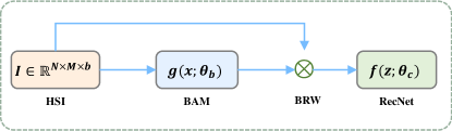
Figure 2: Overview of Band Selection Networks: A given HSI data is first passed onto a Band Attention Module (BAM) to explicitly model the nonlinear interdependencies between spectral bands. Then, the input HSI is re-weighted band-wisely by a Band Re-weighting (BRW) operation. Finally, a Reconstruction Network (RecNet) is conducted to restore the original spectral bands from the re-weighted bands.

III BS-Nets

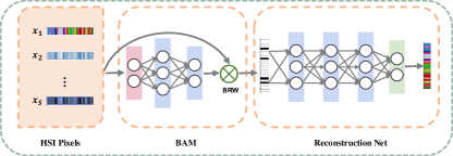
(a) BS-Net-FC.

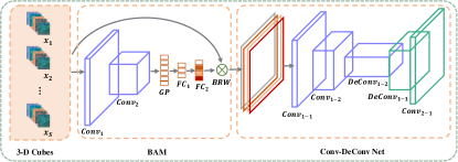
(b) BS-Net-Conv.

Figure 3: Implementation details of BS-Nets based on different networks. (a) BS-Net based on fully connected networks with spectral inputs. (b) BS-Net based on convolutional neural networks with spectral-spatial inputs.

In this section, we first introduce the main components included in the BS-Nets general architecture. Then, we give two versions of implementations of the BS-Nets based on fully connected networks and convolutional neural networks, respectively. Finally, we show a discussion on the BS-Nets.

III-A Architecture of BS-Nets

The key to the BS-Nets is to convert the band selection as a sparse band reconstruction task, i.e., recover the complete spectral information using a few informative bands. For a given spectral band, if it is informative then it will be essential for a spectral reconstruction. To this end, we design a deep neural network based on the attention mechanism. In Fig. 2, we show the overall architecture of the proposed framework, which consists of three components: band attention module (BAM), band re-weighting (BRW), and reconstruction network (RecNet). The detailed introduction is given as follows.

The BAM is a branch network which we use to learn the band weights. As shown in Fig. 2, BAM directly takes HSI as input and aims to fully extract the interdependencies between spectral bands. We express BAM as a function $g$ that takes a certain HSI cube $\boldsymbol{x}$ as input and produces a non-negative band weights tensor, $\boldsymbol{w}\in\mathbb{R}^{1\times 1\times b}$.

$$\boldsymbol{w}=g\left(\boldsymbol{x};\boldsymbol{\varTheta}_{b}\right)$$ (5)

Here $\boldsymbol{\varTheta}_{b}$ denotes the trainable parameters involved in the BAM. To guarantee the non-negativity of the learned weights, Sigmoid function is adopted as the activation of the output layer in BAM, which is written as:

$$\phi\left(\boldsymbol{w}\right)=\frac{1}{1+e^{-\boldsymbol{w}}}$$ (6)

To create an interaction between the original inputs and their weights, a band-wise multiplication operation is conducted. We refer to this operation as BRW. It can be explicitly represented as follows.

$$\mathbf{z}=\boldsymbol{x}\otimes\boldsymbol{w}$$ (7)

Where $\otimes$ indicates the band-wise production between $\boldsymbol{x}$ and $\boldsymbol{w}$, and $\mathbf{z}$ is the re-weighted counterpart of the input $\boldsymbol{x}$.

In the next step, we employ the RecNet to recover the original spectral band from the re-weighted counterpart. Similarly, we define the RecNet as a function $f$ that takes a re-weighted tensor $\mathbf{z}$ as input and outputs its prediction.

$$\hat{\boldsymbol{x}}=f\left(\mathbf{z};\boldsymbol{\varTheta}_{c}\right)$$ (8)

Where $\hat{\boldsymbol{x}}$ is the prediction output for the original input $\boldsymbol{x}$, and $\boldsymbol{\varTheta}_{c}$ denotes the trainable parameters involved in RecNet.

In order to measure the reconstruction performance, we use the Mean-Square Error (MSE) as the cost function, denoted as $\mathcal{L}$. We define it as follows:

$$\mathcal{L}=\frac{1}{2S}\stackrel{{\scriptstyle[}}{{i}}=1]{S}{\sum}\left\|\boldsymbol{x}_{i}-\hat{\boldsymbol{x}}_{i}\right\|_{2}^{2}$$ (9)

Here $S$ is the number of training samples. Moreover, we desire to keep the band weights as sparse as possible such that we can interpret them more easily. For this purpose, we impose an $L_{1}$ norm constraint on the band weights. The resulting loss function is given as follows:

$$\mathcal{L}\left(\boldsymbol{\varTheta}_{b},\boldsymbol{\varTheta}_{c}\right)=\frac{1}{2S}\stackrel{{\scriptstyle[}}{{i}}=1]{S}{\sum}\left\|\boldsymbol{x}_{i}-\hat{\boldsymbol{x}}_{i}\right\|_{2}^{2}+\lambda\stackrel{{\scriptstyle[}}{{i}}=1]{S}{\sum}\left\|\boldsymbol{w}_{i}\right\|_{1}$$ (10)

Where $\lambda$ is a regularization coefficient which balances the minimization between the reconstruction error and regularization term. Eq. (10) can be optimized by using a gradient descent method, such as Stochastic Gradient Descent (SGD) and Adaptive Moment Estimation (Adam).

According to the learned sparse band weights, we can determine the informative bands by averaging the band weights for all the training samples. The average weight of the $j$-th band is computed as:

$$\overline{w}_{j}=\frac{1}{S}\stackrel{{\scriptstyle[}}{{i}}=1]{S}{\sum}\boldsymbol{w}_{ij}$$ (11)

Those bands which have larger average weights are considered to be significant since they make more contributions to the reconstruction. In practice, the top $k$ bands are selected as the significant band subset. The pseudocode of BS-Nets is given in Algorithm 1.

Input: HSI cube: $\boldsymbol{I}\in\mathbb{R}^{N\times M\times b}$; Band subset size: $k$; and BS-Nets hyper-parameters.

Output: Informative band subset.

1 Preprocess HSI and generate training samples;

2 Random initialize $\boldsymbol{\varTheta}_{b}$ and $\boldsymbol{\varTheta}_{c}$ according to the given network configure;

3 while Model is convergent or maximum iteration is met do

4       Sample a batch of training samples $\boldsymbol{x}$;

5       Calculate bands weights: $\boldsymbol{w}=g\left(\boldsymbol{x};\boldsymbol{\varTheta}_{b}\right)$;

6       Re-weight spectral bands: $\mathbf{z}=\boldsymbol{x}\otimes\boldsymbol{w}$;

7       Reconstruct spectral bands: $\hat{\boldsymbol{x}}=f\left(\mathbf{z};\boldsymbol{\varTheta}_{c}\right)$;

8       Update $\boldsymbol{\varTheta}_{b}$ and $\boldsymbol{\varTheta}_{c}$ by minimizing Eq.(10) using Adam algorithm;

9      

10 end while

11Calculate average band weights according to Eq. (11);

12 Select top $k$ bands;

Algorithm 1 Pseudocode of BS-Nets

III-B BS-Net Based on Fully Connected Networks (BS-Net-FC)

In Fig. 3 (a), we show the first implementation of BS-Net based on fully modeling the nonlinear relationship between the spectral information. In this case, both of BAM and RecNet are implemented with fully connected networks, and thus we refer to this BS-Net as BS-Net-FC.

As illustrated in Fig. 3 (a), the BAM is designed as a bottleneck structure with multiple fully connected layers, with ReLu activations for all the middle hidden layers. According to the information bottleneck theory [44], bottleneck structure would be favorable for the extraction of information, although different structures are allowed in BS-Nets.

In BS-Net-FC, we use spectral vectors (pixels) as the training samples. For convenience, we denote the training set comprising $S$ samples as a 4-D tensor $\mathbf{X}\in\mathbb{R}^{S\times 1\times 1\times b}$, where $S=M\times N$. By rewriting the band weights in the tensor form, represented as $\mathbf{W}\in\mathbb{R}^{S\times 1\times 1\times b}$, the BRW is actually an element-wise production operation that can be written as $\mathbf{Z}=\mathbf{X}\otimes\mathbf{W}$, where $\mathbf{Z}$ is the re-weighted spectral inputs. In RecNet, we use a simple multi-layer perceptron model with the same number of hidden neurons with ReLu activations to reconstruct spectral information.

III-C BS-Net Based on Convolutional Networks (BS-Net-Conv)

During the training in BS-Net-FC, only the spectral information is taken into account. The lack of consideration for the spatial information would result in low-efficiency use of the spectral-spatial information containing in HSI. To enhance the BS-Net-FC, we implement the second BS-Net by using convolutional networks, which is termed as BS-Net-Conv. The schematic of the implementation is given in Fig. 3 (b).

In the BAM, we first employ several 2-D convolutional layers to extract spectral and spatial information simultaneously. Then, a global pooling (GP) layer is used to reduce the spatial size of the resulting feature maps. Finally, the final band weights $\mathbf{W}$ is generated by a few fully connected layer and used to reweight the spectral bands. BS-Net-Conv adopts a convolutional-deconvolutional network (Conv-DeConv Net) to implement the RecNet. Similar to the classical auto-encoder, Conv-DeConv Net includes a convolutional encoder which extracts deep features and a deconvolutional decoder which up-samples feature maps.

Instead of using single pixels, BS-Net-Conv takes 3-D HSI patches which includes spectral and spatial information as the training samples. To generate enough training samples, we use a rectangular window of size $a\times a$ to slides across the given HSI with stride $t$. The generated training samples can be denoted as $\mathbf{X}\in\mathbb{R}^{S\times a\times a\times b}$, where $S=\frac{M-a}{t}\times\frac{N-a}{t}+1$. Notice that the number of training samples in BS-Net-Conv is less than that in BS-Net-FC.

III-D Remarks on BS-Net framework

The key to our proposed BS-Net framework is to use deep neural networks to explicitly learn spectral bands weights. Compared with the existing band selection methods, the framework has the following advantages. The first is the framework is end-to-end trainable, making it easy to combine with specific tasks and existed neural networks, such as deep learning based HSI classification. The second is the framework is capable of adaptively exacting spectral and spatial information, which avoids hand-designed features and reduces the noise effect. The third is the framework is nonlinear, enabling it to make full exploration of the nonlinear relationship between bands. The fourth is the framework is flexible to be implemented with diverse networks.

TABLE I: Summary of Indian Pines, Pavia University, and Salinas data sets.

Data sets	Indina Pines	Pavia University	Salinas
Pixels	145$\times$145	610$\times$340	512$\times$217
Channels	200	103	204
Classes	16	9	16
Labeled pixels	10249	42776	54129
Sensor	AVIRIS	ROSIS	AVIRIS

TABLE II: Hyper-parameters settings for different BS methods.

Baselines	Hyper-parameters
ISSC	$\lambda=1e5$
SpaBS	$\lambda=1e2$
MVPCA	–
SNMF	$maxiter=100$
MOBS	$maxiter=100$,$NP=100$
OPBS	–
BS-Net-FC	$\lambda=1e-2$,$\eta=2e-3$,$maxiter=100$
BS-Net-Conv	$\lambda=1e-2$,$\eta=2e-3$,$maxiter=100$

TABLE III: Configuration of BS-Net-FC for Indian Pines data set.

Branch	Layer	Hidden Neurons	Activation
BAM	Input	200	–
	FC1-1	64	ReLU
	FC1-2	128	ReLU
	FC1-3	200	Sigmoid
RecNet	FC2-1	64	ReLU
	FC2-2	128	ReLU
	FC2-3	256	ReLU
	FC2-4	200	Sigmoid

TABLE IV: Configuration of BS-Net-Conv for Indian Pines data set.

Branch	Layer	Kernel	Activation
BAM	Conv1	$3\times 3\times 64$	ReLU
	GP	–	–
	FC1	128	ReLU
	FC2	200	Sigmoid
RecNet	Conv1-1	$3\times 3\times 128$	ReLU
	Conv1-2	$3\times 3\times 64$	ReLU
	DeConv1-2	$3\times 3\times 64$	ReLU
	DeConv1-1	$3\times 3\times 128$	ReLU
	Conv2-1	$1\times 1\times 200$	Sigmoid

IV Results

IV-A Setup

In this section, we will widely evaluate the performance of the proposed BS-Nets on three real HSI data sets: Indian Pines, Pavia University, and Salinas. The summary of the three data sets is shown in Table I. For each data set, we first investigate the model convergence by analyzing the training loss, classification accuracy, and band weights. Next, we compare the classification performance for BS-Nets with many existing band selection methods, i.e., ISSC [10], SpaBS [20], MVPCA [19], SNMF [18], MOBS [5], and OPBS [22]. The hyper-parameters settings of all the methods are listed in Table II. To better demonstrate the performance, we also compare with all bands. Finally, we make a deep analysis on the selected band subsets from aspects of visualization and quantification.

Similar to the evaluation strategy adopted in [5, 22], we use Support Vector Machine (SVM) with radial basis function kernel as the classifier to evaluate the classification performance of the selected band subsets. For the sake of fairness, we randomly select $5\%$ of labeled samples from each data set for training set, and the rest for testing set. Three popular quantitative indices, i.e., Overall Accuracy (OA), Average Accuracy (AA), and Kappa coefficient (Kappa) are calculated by evaluating each BS method for $20$ independent runs.

To quantitatively analyze the selected band subsets, the entropy and mean spectral divergence (MSD) [45, 5] of band subsets are calculated. For a single band $\boldsymbol{B}_{i}$, its entropy is defined as follows:

$$H\left(\boldsymbol{B}_{i}\right)=-\underset{y\in\Psi}{\sum}p\left(y\right)\log\left(p\left(y\right)\right)$$ (12)

Here $y$ denotes a gray level of the histogram of the $i$-th band $\boldsymbol{B}_{i}$, and $p\left(y\right)=\frac{n\left(y\right)}{N\times M}$ indicates the ratio (probability) of the number of $y$ to that all pixels. According to the characteristic of entropy, the larger the entropy is, the more image details the band contains [5]. The MSD is an average measurement index for a band subset $\boldsymbol{B}$, which is expressed as:

$$M\left(\boldsymbol{B}\right)=\frac{2}{k\left(k-1\right)}\stackrel{{\scriptstyle[}}{{i}}=1]{k}{\sum}\stackrel{{\scriptstyle[}}{{j}}=1]{k}{\sum}D_{SKL}\left(\boldsymbol{B}_{i}\parallel\boldsymbol{B}_{j}\right)$$ (13)

Where $D_{SKL}$ is the symmetrical Kullback–Leibler divergence which measures the dissimilarity between $\boldsymbol{B}_{i}$ and $\boldsymbol{B}_{j}$. Specifically, $D_{SKL}$ is defined as follows:

$$D_{SKL}\left(\boldsymbol{B}_{i}\parallel\boldsymbol{B}_{j}\right)=D_{KL}\left(\boldsymbol{B}_{i}\parallel\boldsymbol{B}_{j}\right)+D_{KL}\left(\boldsymbol{B}_{j}\parallel\boldsymbol{B}_{i}\right)$$ (14)

Here $D_{KL}\left(\boldsymbol{B}_{i}\parallel\boldsymbol{B}_{j}\right)$ can be computed from the gray histogram information. From Eq. (13), MSD evaluates the redundancy among the selected bands, that is, the larger the value of the MSD is, the less redundancy is contained among the selected bands.

The configuration of BS-Nets implemented in our experiments are shown in Table III and Table IV. In reprocessing, we scale all the HSI pixel values to the range $\left[0,1\right]$. All the baseline methods are evaluated with Python 3.5 running on an Intel Xeon E5-2620 2.10 GHz CPU with 32 GB RAM. In addition, we implement BS-Nets with TensorFlow-GPU 1.6 and accelerate them on a NVIDIA TITAN Xp GPU with 11 GB graphic memory. One may refer to https://github.com/AngryCai for the source codes and trained models.

IV-B Results on Indian Pines Data Set

IV-B1 Data Set

This scene was gathered by AVIRIS sensor over the Indian Pines test site in North-western Indiana and consists of $145\times 145$ pixels and $224$ spectral reflectance bands in the wavelength range $0.4\text{\textendash}2.5$ $\left(\times 10^{-6}\right)$ meters. The scene contains two-thirds agriculture, and one-third forest or other natural perennial vegetation. There are two major dual lane highways, a rail line, as well as some low-density housing, other built structures, and smaller roads. Since the scene is taken in June some of the crops presents, corn, soybeans, are in early stages of growth with less than $5\%$ coverage. The ground-truth available is designated into sixteen classes and is not all mutually exclusive. We have also reduced the number of bands to $200$ by removing bands covering the region of water absorption: $[104-108]$, $[150-163]$, $220$.

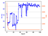
(a) BS-Net-FC

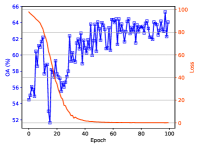
(b) BS-Net-Conv

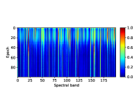
(c) BS-Net-FC

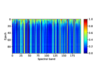
(d) BS-Net-Conv

Figure 4: Analysis of the convergence of BS-Nets on Indian Pines data set. Visualization of loss versus accuracy under different iterations for (a) BS-Net-FC and (b) BS-Net-Conv. Visualization of average band weights under varying iterations for (c) BS-Net-FC and (d) BS-Net-Conv.

IV-B2 Analysis of Convergence of BS-Nets

To analyze the convergence of BS-Nets, we train BS-Nets for 100 iterations and plot their training loss curves and classification accuracy using the best $5$ significant bands. The results of BS-Net-FC and BS-Net-Conv are shown in Fig. 4 (a) and (b), respectively. Observing from Fig. 4 (a)-(b), the reconstruction errors decrease with iterations, and at the same time, the classification accuracies increase. The loss values of BS-Net-FC is very close to zero after 20 iterations and the classification accuracy finally stabilizes around $63\%$ after 40 interactions. The similar trend can be found from BS-Net-Conv, showing that the proposed BS-Nets are easy to train with high convergency speed. Furthermore, we can find that the classification accuracy is increased from $42\%$ to $63\%$ for BS-Net-FC and $52\%$ to $64\%$ for BS-Net-Conv. Therefore, the well-optimized BS-Nets can respectively achieve $21\%$ and $12\%$ improvement in terms of classification accuracy, which demonstrates the effectiveness of the proposed BS-Nets.

We further visualize the average band weights obtained by BS-Net-FC and BS-Net-Conv with different iterations in Fig. 4 (c) and (d). To better show the change trend of band weights, we scale these weights into range $\left[0,1\right]$. The horizontal and vertical axis represent the band number and iterations, respectively, where each column depicts the change of one band’s weights. As we can see, the the band weights distribution becomes gradually sparser and sparser. Meanwhile, the informative bands become easier to be distinguished due to the trivial bands will finally be assigned with very small weights.

IV-B3 Performance Comparison

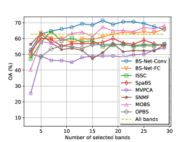
(a) OA

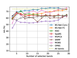
(b) AA

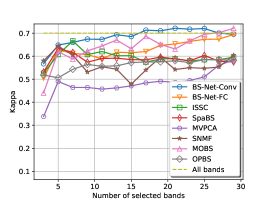
(c) Kappa

Figure 5: Performance comparison of different BS methods with different band subset sizes on Indian Pines data set. (a) OA; (b) AA; (c) Kappa.

To demonstrate the effectiveness of both BS-Nets, we compare the classification performance of different BS methods under different band subset sizes. Three indices, i.e., OA, AA, and Kappa, are computed under band subset sizes ranging from 3 to 30 with 2-band interval. All bands performance is also compared as an important reference. To ensure a reliable classification result, we conduct each method for 20 times and randomly select the training set and test set during each time. Fig. 5 (a)-(c) shows the average comparison results of OA, AA, and Kappa, respectively. From Fig. 5 (a)-(c), BS-Net-Conv achieves the best OA, AA, and Kappa when the band subset size is larger than $5$, while BS-Net-FC achieves comparable performance with MOBS but is superior to the other 5 competitors. BS-Net-Conv respectively requires $5$, $17$, and $17$ bands to achieve better OA, AA, and Kappa than all bands, while other methods either worst than all bands or have to use more bands. Notice that a counter-intuitive phenomenon that the classification performance is not always increased by selecting more bands can be found from the results. For example, ISSC and SNMF display significant decreasing trend when the band subset size is over $7$. The phenomenon can be explained as the so-called Hughes phenomenon [46], i.e., the classification accuracy increases first and then decreases with the selected bands. However, even if so, BS-Net occurs the phenomenon obviously later than other methods, which means our methods are able to select more effective band subset.

TABLE V: Classification performance of different methods using 15 bands on Indian Pines data set.

No.	#Train	#Test	ISSC	SpaBS	MVPCA	SNMF	MOBS	OPBS	BS-Net-FC	BS-Net-Conv
1	2	44	31.14$\pm$21.19	27.24$\pm$27.72	19.43$\pm$13.84	14.29$\pm$16.18	55.03$\pm$20.82	34.97$\pm$24.82	38.98$\pm$22.78	66.41$\pm$24.59
2	71	1357	64.13$\pm$3.21	60.35$\pm$4.34	48.13$\pm$4.04	57.36$\pm$4.90	65.56$\pm$3.12	59.46$\pm$4.19	67.49$\pm$4.37	75.67$\pm$2.91
3	41	789	52.17$\pm$5.64	53.62$\pm$3.35	35.68$\pm$3.80	47.56$\pm$4.82	58.19$\pm$4.96	48.60$\pm$5.08	59.62$\pm$3.79	64.39$\pm$5.30
4	12	225	36.78$\pm$8.34	39.28$\pm$10.40	12.74$\pm$5.34	35.64$\pm$7.87	46.60$\pm$11.09	31.24$\pm$10.50	40.08$\pm$8.26	61.41$\pm$12.18
5	24	459	73.98$\pm$8.39	81.16$\pm$3.46	62.32$\pm$8.33	70.39$\pm$8.17	79.39$\pm$5.52	79.79$\pm$5.17	80.90$\pm$5.41	85.78$\pm$4.22
6	37	693	83.49$\pm$3.94	82.21$\pm$7.18	83.08$\pm$4.36	75.41$\pm$6.43	88.57$\pm$4.69	89.02$\pm$3.78	90.93$\pm$4.66	93.63$\pm$2.53
7	1	27	29.55$\pm$28.04	37.97$\pm$22.80	19.79$\pm$18.58	12.99$\pm$15.46	39.16$\pm$32.62	29.11$\pm$23.12	52.44$\pm$28.16	45.30$\pm$39.45
8	24	454	88.33$\pm$4.63	86.75$\pm$10.38	85.15$\pm$5.65	88.08$\pm$6.45	92.04$\pm$5.84	90.68$\pm$5.47	93.77$\pm$4.85	96.86$\pm$2.82
9	1	19	10.91$\pm$12.80	6.88$\pm$9.32	7.55$\pm$10.33	7.31$\pm$10.62	48.27$\pm$31.66	7.46$\pm$10.87	24.26$\pm$22.49	28.07$\pm$35.09
10	49	923	52.69$\pm$3.87	53.21$\pm$5.10	40.71$\pm$4.74	50.07$\pm$5.73	52.34$\pm$5.33	52.27$\pm$5.09	60.72$\pm$4.19	66.45$\pm$5.52
11	123	2332	62.14$\pm$2.39	57.87$\pm$2.42	50.58$\pm$3.07	56.52$\pm$2.91	62.10$\pm$3.81	61.37$\pm$3.68	67.04$\pm$3.69	71.69$\pm$2.91
12	30	563	35.02$\pm$5.38	43.15$\pm$7.78	34.44$\pm$6.57	31.09$\pm$5.28	57.20$\pm$8.34	30.52$\pm$5.29	42.95$\pm$6.48	65.30$\pm$5.76
13	10	195	86.78$\pm$8.03	91.18$\pm$7.31	82.45$\pm$8.59	81.06$\pm$10.54	91.73$\pm$5.11	80.96$\pm$12.79	93.75$\pm$4.92	94.35$\pm$6.33
14	63	1202	85.76$\pm$3.50	89.83$\pm$2.32	85.94$\pm$3.48	86.17$\pm$3.64	86.99$\pm$3.57	86.44$\pm$5.21	89.08$\pm$3.49	89.46$\pm$3.07
15	19	367	31.21$\pm$7.32	32.80 $\pm$7.44	29.4$\pm$4.76	29.08$\pm$7.53	36.90$\pm$8.13	31.73$\pm$8.20	39.91$\pm$8.07	47.53$\pm$10.18
16	5	88	80.76$\pm$18.76	71.1$\pm$21.56	76.28$\pm$8.33	82.98$\pm$5.47	81.76$\pm$5.3	80.86$\pm$7.46	81.90$\pm$6.22	76.98$\pm$21.11
OA (%)			56.55$\pm$2.47	57.16$\pm$2.25	48.35$\pm$1.92	51.62$\pm$2.02	65.11$\pm$2.76	55.90$\pm$2.39	63.99$\pm$2.51	70.58$\pm$2.87
AA (%)			63.91$\pm$0.73	63.78$\pm$0.99	54.87$\pm$1.59	59.75$\pm$1.15	67.54$\pm$0.83	63.13$\pm$1.09	69.58$\pm$1.00	75.53$\pm$0.69
Kappa			0.589$\pm$0.008	0.588$\pm$0.011	0.486$\pm$0.018	0.542$\pm$0.013	0.631$\pm$0.009	0.580$\pm$0.012	0.653$\pm$0.011	0.721$\pm$0.008

In Table V, we show the detailed classification performance of selecting best $19$ bands for different methods. As we can see, BS-Net-FC and BS-Net-Conv outperform all the competitors in terms of OA, AA, Kappa. For some classes which contain limited training samples, such as No. 7 and No. 9 class, BS-Net-FC and BS-Net-Conv can still yield much better or comparable accuracy compared with the other methods. Compared with BS-Net-FC, BS-Net-Conv achieves $6.59\%$ improvement in terms of OA, showing that spectral-spatial information is more effective for band selection than using only spectral information.

IV-B4 Analysis of the Selected Bands

TABLE VI: The best 15 bands of Indian Pines data set selected by different BS methods.

Methods	Selected Bands
BS-Net-FC	[165, 38, 51, 65, 12, 100, 0, 71, 5, 60, 88, 26, 164, 75, 74]
BS-Net-Conv	[46,33,140,161,80,35,178,44,126,36,138,71,180,66,192]
ISSC	[171,130,67,85,182,183,47,143,138,90,139,141,25,142,21]
SpaBS	[7, 96, 52, 171, 53, 3, 76, 75, 74, 95, 77, 73, 78, 54, 81]
MVPCA	[167,74,168,0,147,165,161,162,152,19,160,119,164,159,157]
SNMF	[23,197,198,94,76,2,87,105,143,145,11,84,132,108,28]
MOBS	[5,6,19,24,45,48,105,114,129,142,144,160,168,172,181]
OPBS	[28, 41, 60, 0, 74, 34, 88, 19, 17, 33, 56, 87, 22, 31, 73]

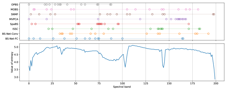
Figure 6: The best 15 bands of Indian Pines data set selected by different BS methods (above) and the entropy value of each band (below).

We extensively analyze the selected bands in this section. Table VI gives the best $15$ bands of Indian Pines data set selected by different methods. To better show the band distribution, we indicate the locations of these bands on the spectrum in Fig. 6 (above). Each row represents a BS method with its corresponding locations of the selected bands. As we can see, the results obtained by both BS-Nets contain less continuous bands with a relatively uniform distribution. Basing on the fact that the adjacent bands generally include higher correlation and thus less redundancy containing among the band subsets selected by both BS-Nets. Furthermore, we analyze these bands from the perspective of the information entropy which we show in Fig. 6 (below). Those bands with extremely low entropy compared with their adjacent bands can be regarded as noisy bands with little information, i.e., $\left[104,105\right]$, $\left[144,145\right]$, $\left[198,199,200\right]$. It can be seen that both BS-Nets avoid these regions with low entropy since these noisy bands make no contribution to the spectral reconstruction. Instead, both BS-Nets select informative bands from relatively smooth regions with high entropy, thereby reducing the redundancy.

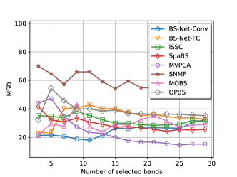
Figure 7: Mean Spectral Divergence values of different BS methods on Indian Pines data set.

In Fig. 7, we show the MSDs of different BS methods under different band subset size. From Fig. 7, BS-Net-FC has comparable MSD values with OPBS but is better than most of the competitors, i.e., ISSC, SpaBS, MVPCA, and MPBS. Although BS-Net-Conv achieves the best classification performance, it does not achieve the best MSD. As analyzed in [5], the reason for this phenomenon is that the MSD will also increase if noisy bands are selected, which can be concluded from Eq. (13). For instance, the MSDs of band subsets $\left[104,144\right]$ and $\left[104,25\right]$ are $106.64$ and $51.49$, respectively. It is obvious that $\left[104,144\right]$ shows much better MSD value than $\left[104,25\right]$, however, $\left[104,144\right]$ contains two completely noisy bands which makes less sense to the classification.

IV-C Results on Pavia University Data Set

IV-C1 Data Set

Pavia University data set was acquired by the ROSIS sensor during a flight campaign over Pavia, northern Italy. This scene is a $103$ spectral bands $610\times 610$ pixels image, but some of the samples in the image contain no information and have to be discarded before the analysis. The geometric resolution is 1.3 meters. The ground-truth differentiates $9$ classes.

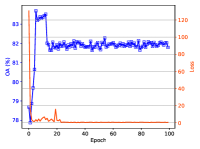
(a) BS-Net-FC

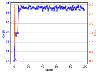
(b) BS-Net-Conv

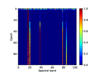
(c) BS-Net-FC

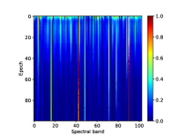
(d) BS-Net-Conv

Figure 8: Analysis of the convergence of BS-Nets on Pavia University data set. Visualization of loss versus accuracy under different iterations for (a) BS-Net-FC and (b) BS-Net-Conv. Visualization of normalized average band weights under varying iterations for (c) BS-Net-FC and (d) BS-Net-Conv.

IV-C2 Analysis of Convergence of BS-Nets

We show the convergence curves and the change trend of band weights in Fig. 8 (a)-(d). From the results, the loss values tend to be zero after several iterations showing that both BS-Nets converge well. Meanwhile, as the increase of iteration, the classification accuracies of the best five bands are increased from $78\%$ to $83\%$ and $72\%$ to $83\%$ for BS-Net-FC and BS-Net-Conv, respectively.

As shown in Fig. 8 (c)-(d), the average band weights become very sparse and easy to distinguish when iteration increases, especially in BS-Net-FC. Finally, only a few significant bands, which are useful to the spectral reconstruction, are highlighted. For example, one can obviously determine that the significant bands of BS-Net-FC are $\left[38,78,17,20,85\right]$ from Fig. 8 (c). Similarly, BS-Net-Conv’s best bands are $\left[90,42,16,48,71\right]$.

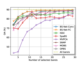
(a) OA

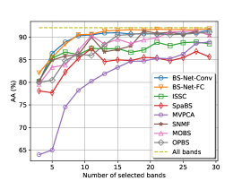
(b) AA

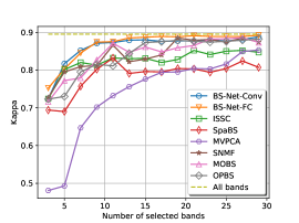
(c) Kappa

Figure 9: Performance comparison of different BS methods with different band subset sizes on Pavia University data set. (a) OA; (b) AA; (c) Kappa.

TABLE VII: Performance comparison of different methods using 15 bands on Pavia University data set.

No.	#Train	#Test	ISSC	SpaBS	MVPCA	SNMF	MOBS	OPBS	BS-Net-FC	BS-Net-Conv
1	373	6258	90.82$\pm$1.23	88.79$\pm$1.37	86.91$\pm$1.18	90.21$\pm$1.11	91.17$\pm$1.33	90.72$\pm$1.32	91.53$\pm$0.80	91.15$\pm$0.88
2	920	17729	95.07$\pm$0.36	95.88$\pm$0.63	94.49$\pm$0.41	96.36$\pm$0.37	95.68$\pm$0.45	95.61$\pm$0.55	96.64$\pm$0.35	95.72$\pm$0.37
3	112	1987	69.65$\pm$3.30	62.98$\pm$3.05	57.06$\pm$4.59	72.77$\pm$3.00	70.97$\pm$2.88	73.60$\pm$3.13	72.30$\pm$2.94	71.20$\pm$3.01
4	134	2930	89.29$\pm$2.07	85.10$\pm$1.66	79.86$\pm$2.38	89.37$\pm$1.49	89.00$\pm$1.68	89.72$\pm$1.97	91.47$\pm$1.78	90.60$\pm$1.78
5	69	1276	98.89$\pm$0.35	99.10$\pm$0.27	98.39$\pm$0.67	99.18$\pm$0.39	99.44$\pm$0.20	99.18$\pm$0.50	99.31$\pm$0.30	99.36$\pm$0.28
6	234	4795	74.49$\pm$1.64	52.0$\pm$3.01	72.76$\pm$1.87	85.53$\pm$1.44	78.74$\pm$1.69	84.64$\pm$1.49	86.55$\pm$1.65	84.31$\pm$1.54
7	71	1259	78.89$\pm$4.01	70.63$\pm$6.14	55.44$\pm$6.72	73.47$\pm$4.23	76.62$\pm$4.08	78.90$\pm$3.16	80.66$\pm$2.80	80.01$\pm$3.21
8	179	3503	81.28$\pm$1.83	81.87$\pm$2.45	76.49$\pm$3.61	84.11$\pm$2.55	83.56$\pm$2.18	82.92$\pm$1.60	85.16$\pm$2.30	83.37$\pm$1.96
9	46	901	99.77$\pm$0.16	99.71$\pm$0.14	99.96$\pm$0.15	99.81$\pm$0.17	99.97$\pm$0.07	99.81$\pm$0.14	99.97$\pm$0.05	99.92$\pm$0.08
OA (%)			86.46$\pm$0.54	81.78$\pm$0.89	80.15$\pm$0.68	87.87$\pm$0.58	87.24$\pm$0.59	88.34$\pm$0.62	89.29$\pm$0.47	88.40$\pm$0.51
AA (%)			88.86$\pm$0.28	85.42$\pm$0.33	85.35$\pm$0.22	90.76$\pm$0.26	89.87$\pm$0.27	90.65$\pm$0.37	91.77$\pm$0.30	90.87$\pm$0.28
Kappa			0.852$\pm$0.004	0.803$\pm$0.005	0.804$\pm$0.003	0.877$\pm$0.003	0.865$\pm$0.004	0.876$\pm$0.005	0.891$\pm$0.004	0.879$\pm$0.004

IV-C3 Performance Comparison

In this experiment, we perform different BS methods to select different sizes of band subsets ranging from 3 to 30. We show the obtained OAs, AAs, and Kappas in Fig. 9 (a)-(c). When band subset size is less than $17$, both BS-Nets have similar classification performance and are significantly superior to the other BS methods in terms of all the three indices. When band subset size is larger than $17$, BS-Net-FC achieves the best classification performance, while BS-Net-Conv achieves comparable performance with SNMF and OPBS. Using only $25$ bands, both BS-Nets show comparable performance with all bands and no obvious Hughes phenomenon.

In Table VII, we compare the detailed classification performance by setting the band subset size to $19$. From Table VII, both BS-Nets achieve the best OA, AA, and Kappa by comparing with the other competitors. In addition, BS-Net-FC wins in $7$ classes in terms of classes accuracy. For the two failed classes, i.e., No. 3 and No. 5 classes, their classification accuracy are superior to most of the other competitors. Especially on No. 3 class, which is relatively difficult to classify, but both BS-Nets also achieve much more accurate results than ISSC, SpaBS, and MVPCA.

IV-C4 Analysis of the Selected Bands

TABLE VIII: The best 15 bands of Pavia University data set selected by different BS methods.

Methods	Selected Bands
BS-Net-FC	[38, 78, 17, 20, 85, 98, 65, 81, 79, 90, 95, 74, 66, 62, 92]
BS-Net-Conv	[90, 42, 16, 48, 71, 3, 78, 38, 80, 53, 7, 31, 4, 99, 98]
ISSC	[51, 76, 7, 64, 31, 8, 0, 24, 40, 30, 5, 3, 6, 27, 2]
SpaBS	[50, 48, 16, 22, 4, 102, 21, 25, 23, 47, 24, 20, 31, 26, 42]
MVPCA	[48, 22, 51, 16, 52, 21, 65, 17, 20, 53, 18, 54, 19, 55, 76]
SNMF	[92, 53, 43, 66, 22, 89, 82, 30, 51, 5, 83, 77, 80, 2, 48]
MOBS	[4, 15, 23, 25, 33, 35, 42, 53, 58, 61, 62, 64, 67, 73, 101]
OPBS	[90, 62, 14, 0, 2, 72, 102, 4, 33, 1, 6, 84, 45, 82, 8]

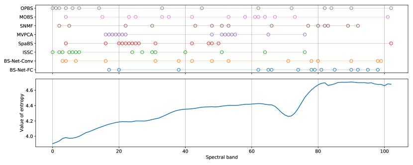
Figure 10: The best 15 bands of Pavia University data set selected by different BS methods (above) and the entropy value of each band (below).

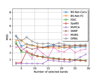
Figure 11: Mean Spectral Divergence values of different BS methods on Pavia University data set.

The best $15$ bands selected by different BS methods are listed in Table VIII. Fig. 10 shows the corresponding band indices and the entropy value of each spectral band. The entropy curve of this data set is relatively smooth without rapidly decreasing regions and moreover increases with spectral bands. Compared with the competitors, the band subsets selected by both BS-Nets contain fewer continuous bands and are more concentrated around the positions of larger entropy. In contrast, MVPCA, SpaBS, and ISSC include more adjacent bands at the region with low entropy. As a result, these methods have worse classification performance than BS-Nets. The MSD values of the different BS methods are given in Fig. 11. It can be seen that both BS-Nets are comparable with OPBS and are better than ISSC, SpaBS, MVPCA, and MOBS, showing that the selected band subsets contain less redundant bands.

IV-D Results on Salinas Data Set

IV-D1 Data set

This scene was collected by the 224-band AVIRIS sensor over Salinas Valley, California, and is characterized by high spatial resolution ($3.7$-meter pixels). The area covered comprises $512\times 217$ samples. As with Indian Pines scene, we discarded the 20 water absorption bands, in this case, bands: $[108-112]$, $[154-167]$, $224$. It includes vegetables, bare soils, and vineyard fields. Salinas ground-truth contains 16 classes.

IV-D2 Analysis of Convergence of BS-Nets

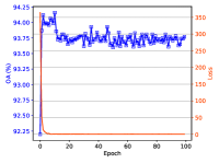
(a) BS-Net-FC

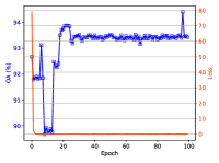
(b) BS-Net-Conv

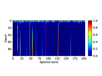
(c) BS-Net-FC

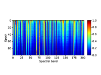
(d) BS-Net-Conv

Figure 12: Analysis of the convergence of BS-Nets on Salinas data set. Loss versus accuracy under different iterations for (a) BS-Net-FC and (b) BS-Net-Conv. Visualization of normalized average band weights under varying iterations for (c) BS-Net-FC and (d) BS-Net-Conv.

Fig. 12 (a)-(b) show the convergence curves of BS-Nets on Salinas data set. Training about $20$ iterations, BS-Nets’ loss and accuracy have tended to be convergent. The OA of using $5$ bands are increased from $92\%$ to $94\%$ and from $85\%$ to $94\%$ for BS-Net-FC and BS-Net-Conv, respectively. In Fig. 12 (c)-(d), we show the means of band weights under different iterations. Similar to Indian Pines and Pavia University data sets, the learned band weights become sparse with the increase of iterations.

IV-D3 Performance Comparison

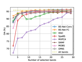
(a) OA

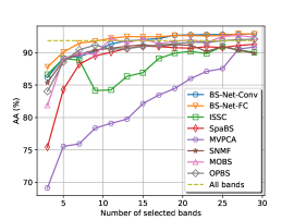
(b) AA

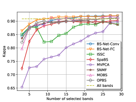
(c) Kappa

Figure 13: Performance comparison of different BS methods with different band subset sizes on Salinas data set. (a) OA; (b) AA; (c) Kappa.

TABLE IX: Performance comparison of different methods using 15 bands on Salinas data set.

NO.	#Train	#Test	ISSC	SpaBS	MVPCA	SNMF	MOBS	OPBS	BS-Net-FC	BS-Net-Conv
1	100	1909	99.08$\pm$0.49	99.25$\pm$0.27	98.99$\pm$0.50	99.24$\pm$0.46	98.69$\pm$0.72	98.76$\pm$0.68	99.32$\pm$0.55	99.39$\pm$0.31
2	179	3547	99.72$\pm$0.34	99.55$\pm$0.23	98.47$\pm$0.57	99.64$\pm$0.22	99.53$\pm$0.25	99.69$\pm$0.26	99.58$\pm$0.37	99.72$\pm$0.25
3	97	1879	98.20$\pm$0.74	98.49$\pm$0.75	94.20$\pm$2.07	96.74$\pm$1.48	99.08$\pm$0.57	97.20$\pm$1.28	99.30$\pm$0.37	99.25$\pm$0.37
4	77	1317	99.21$\pm$0.62	98.82$\pm$0.76	98.97$\pm$0.93	98.54$\pm$1.08	99.14$\pm$0.65	98.76$\pm$0.82	98.99$\pm$0.61	98.64$\pm$1.01
5	117	2561	98.42$\pm$0.58	98.19$\pm$0.49	94.78$\pm$0.74	96.29$\pm$1.19	97.98$\pm$0.62	96.96$\pm$1.14	97.98$\pm$0.80	98.39$\pm$0.65
6	204	3755	99.88$\pm$0.06	99.78$\pm$0.15	99.38$\pm$0.22	99.74$\pm$0.13	99.77$\pm$0.09	99.79$\pm$0.09	99.79$\pm$0.11	99.79$\pm$0.12
7	180	3399	99.62$\pm$0.23	99.43$\pm$0.28	98.90$\pm$0.61	99.45$\pm$0.29	99.59$\pm$0.18	99.56$\pm$0.22	99.58$\pm$0.23	99.56$\pm$0.15
8	585	10686	82.18$\pm$1.76	85.51$\pm$1.52	83.51$\pm$1.32	85.08$\pm$1.50	86.24$\pm$1.23	85.06$\pm$1.71	87.27$\pm$1.60	88.15$\pm$1.13
9	305	5898	99.30$\pm$0.38	99.2$\pm$0.38	94.14$\pm$1.16	99.24$\pm$0.39	98.94$\pm$0.62	99.06$\pm$0.73	99.34$\pm$0.38	99.46$\pm$0.42
10	179	3099	93.57$\pm$1.18	90.29$\pm$1.01	85.51$\pm$2.03	90.97$\pm$1.02	93.73$\pm$1.25	91.75$\pm$1.75	94.95$\pm$1.12	94.82$\pm$1.01
11	47	1021	92.69$\pm$2.09	93.73$\pm$2.96	65.59$\pm$3.93	88.35$\pm$4.15	94.21$\pm$1.77	95.33$\pm$2.91	94.09$\pm$3.34	96.19$\pm$1.51
12	117	1810	98.89$\pm$0.92	99.05$\pm$0.61	90.51$\pm$2.81	97.74$\pm$1.03	99.58$\pm$0.33	99.47$\pm$0.54	99.49$\pm$0.88	99.59$\pm$0.71
13	41	875	98.56$\pm$0.80	96.62$\pm$2.35	97.78$\pm$0.93	96.28$\pm$1.96	98.09$\pm$1.34	97.57$\pm$1.85	98.72$\pm$1.25	98.94$\pm$0.85
14	64	1006	94.24$\pm$1.77	95.51$\pm$1.28	95.49$\pm$1.83	92.78$\pm$2.13	95.58$\pm$1.08	94.84$\pm$1.99	96.18$\pm$1.55	96.76$\pm$1.53
15	337	6931	60.42$\pm$3.07	64.81$\pm$2.46	56.20$\pm$2.6 0	62.53$\pm$1.99	69.83$\pm$1.92	70.24$\pm$2.60	71.60$\pm$2.34	70.41$\pm$2.23
16	77	1730	97.60$\pm$0.69	97.55$\pm$0.81	96.19$\pm$1.36	97.59$\pm$0.81	97.76$\pm$0.56	98.88$\pm$0.21	98.08$\pm$0.82	98.65$\pm$0.58
OA (%)			94.47$\pm$0.21	94.74$\pm$0.30	90.54$\pm$0.28	93.76$\pm$0.37	95.48$\pm$0.18	95.18$\pm$0.34	95.89$\pm$0.31	96.11$\pm$0.17
AA (%)			89.85$\pm$0.18	90.90$\pm$0.22	87.10$\pm$0.24	90.19$\pm$0.22	91.97$\pm$0.2	91.60$\pm$0.20	92.61$\pm$0.19	92.74$\pm$0.20
Kappa			0.887$\pm$0.002	0.899$\pm$0.002	0.856$\pm$0.003	0.891$\pm$0.003	0.911$\pm$0.002	0.906$\pm$0.002	0.918$\pm$0.002	0.919$\pm$0.002

The performance comparison of different BS methods on Salinas data set is shown in Fig. 13 (a)-(c). From the results, BS-Net-FC achieves the best classification performance when the band subset size is less than $19$. When band subset size is larger than $19$, both BS-Nets are very comparable in terms of OA, AA, and Kappa, and are significantly better than ISSC, SpaBS, MVPCA, SNMF, and OPBS, as well as all bands. Table IX gives the detailed classification results of using $19$ best bands. It can be seen that both BS-Nets are generally superior to the other BS methods on most of the classes, and significantly outperform all the other BS methods in terms of OA, AA, and Kappa.

IV-D4 Analysis of the Selected Bands

TABLE X: The best 15 bands of Salinas data set selected by different BS methods.

Methods	Selected Bands
BS-Net-FC	[53, 77, 61, 54, 16, 8, 158, 49, 176, 179, 56, 189, 197, 21, 43]
BS-Net-Conv	[116,153,19,189,97,179,171,141,95,144,142,46,104,203,91]
ISSC	[141,182,106,147,107,146,108,202,203,109,145,148,112,201,110]
SpaBS	[0, 79, 166, 80, 203, 78, 77, 76, 55, 81, 97, 5, 23, 75, 2]
MVPCA	[169,67,168,63,68,78,167,166,165,69,164,163,77,162,70]
SNMF	[24, 1, 105, 196, 203, 0, 39, 116, 38, 60, 89, 104, 198, 147]
MOBS	[20,29,35,54,60,62,75,81,93,119,129,132,141,163,201]
OPBS	[44, 31, 37, 66, 11, 1, 164, 2, 18, 0, 3, 40, 4, 54, 33]

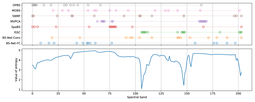
Figure 14: The best 15 bands of Salinas data set selected by different BS methods (above) and the entropy value of each band (below).

Figure 15: Mean Spectral Divergence values of different BS methods on Salinas data set.

The best $15$ bands selected by different BS methods are shown in Table X. Their distribution and entropy are shown in Fig. 14. As we can see, BS-Nets contain less adjacent bands and distribute relatively uniformly. Observing the entropy curve, both BS-Nets can avoid the sharply decreasing regions with low entropy, i.e., $\left[106,107\right]$ and $\left[146,147\right]$. From Fig. 14, some BS methods include a few continuous bands, i.e., OPBS, MVPCA, SpaBS, and ISSC, which means higher correlation is included in their selected band subsets. Fig. 15 shows the MSD values of different BS methods, showing that BS-Net-Conv has comparable MSD with ISSC when the band subset size is larger than $15$. Although SNMF and ISSC achieve the better MSDs, they can not obtain the best classification performance since few of their selected bands locate at noisy regions. Similar to the analysis for Indian Pines data set, these noise bands will increase MSD but reduce the classification performance. In contrast, BS-Net-FC has relative lower MSD, but it completely avoids noisy bands and achieves better classification performance than other BS methods.

IV-E Computational Time Complexity Analysis

To analyze the running time, we conduct all the BS methods on the same computer and collect their absolute running time. MOBS and OPBS are implemented in Matlab and the other methods are implemented in Python. Instead of executing on CPU platform, we train BS-Nets on a GPU platform due to its friendly GPU support. Fig. 16 illustrates the training time of BS-Net-FC and BS-Net-Conv trained on Indian Pines data set with different iterations. According to the implementation details shown in Table III-IV, BS-Net-FC and BS-Net-Conv include about $152,592$ and $590,288$ trainable parameters, respectively. However, the number of training samples used in BS-Net-FC is $21025$ while that in BS-Net-Conv is $4489$. It can be seen from Fig. 16, BS-Net-Conv saves about half of the time cost by comparing with BS-Net-FC. It is interesting to notice that the training time is approximatively linear to the iterations.

Table XI shows the computational time of selecting $19$ bands using different BS methods on the three data sets. It can be seen that the running times of BS-Nets are comparable with MOBS which bases on heuristic searching and significantly faster than SpaBS and SNMF. Since ISSC and MVPCA can be solved using the algebraic method, they show faster computation speed but cannot achieve better classification performance than BS-Nets. In summary, the proposed BS-Nets are able to balance classification performance and running time.

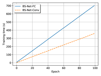
Figure 16: Training time of BS-Nets on Indian Pines data set.

TABLE XI: Computational time (in seconds) for selecting $20$ bands using different BS methods.

Method	Indian Pines	Pavia University	Salinas
ISSC	0.43	14.71	17.44
SpaBS	332.54	2026.80	3224.57
MVPCA	0.44	4.24	7.86
SNMF	$>1h$	$>1h$	$>1h$
MOBS	275.76	289.18	330.30
OPBS	2.00	9.62	9.65
BS-Net-FC	652.08	2015.55	1116.99
BS-Net-Conv	238.04	493.15	444.37

V Conclusions

This paper presents a novel end-to-end band selection network framework for HSI band selection. The main idea behind the framework is to treat HSI band selection as a sparse spectral reconstruction task and to explicitly learn the spectral band’s significance using deep neural networks by considering the nonlinear correlation between spectral bands. The resulting framework allows to learn band weights from full spectral bands, resulting in more efficient use of the global spectral relationship, and consists of two flexible sub-networks, band attention module (BAM) and reconstruction network (RecNet), making it easy to train and apply in practice. The experimental results show that the implemented BS-Net-FC and BS-Net-Conv can not only adaptively produce sparse band weights, but also can significantly better classification performance than many existing BS methods with an acceptable time cost.

We notice that the proposed framework has the capacity of combining with many deep learning based classification methods to reduce computational complexity and enhance the classification performance. That will also be further explored in our future works.

References

- [1] C. M. Gevaert, J. Suomalainen, J. Tang, and L. Kooistra, “Generation of spectral-temporal response surfaces by combining multispectral satellite and hyperspectral uav imagery for precision agriculture applications,” IEEE Journal of Selected Topics in Applied Earth Observations and Remote Sensing, vol. 8, no. 6, pp. 3140–3146, June 2015.
- [2] J. Pontius, R. P. Hanavan, R. A. Hallett, B. D. Cook, and L. A. Corp, “High spatial resolution spectral unmixing for mapping ash species across a complex urban environment,” Remote Sensing of Environment, vol. 199, pp. 360 – 369, 2017.
- [3] B. F. Guolan Lu, “Medical hyperspectral imaging: a review,” Journal of Biomedical Optics, vol. 19, no. 1, pp. 1 – 24 – 24, 2014.
- [4] G. Edelman, E. Gaston, T. van Leeuwen, P. Cullen, and M. Aalders, “Hyperspectral imaging for non-contact analysis of forensic traces,” Forensic Science International, vol. 223, no. 1, pp. 28 – 39, 2012.
- [5] M. Gong, M. Zhang, and Y. Yuan, “Unsupervised band selection based on evolutionary multiobjective optimization for hyperspectral images,” IEEE Transactions on Geoscience and Remote Sensing, vol. 54, no. 1, pp. 544–557, Jan 2016.
- [6] W. Sun and Q. Du, “Graph-regularized fast and robust principal component analysis for hyperspectral band selection,” IEEE Transactions on Geoscience and Remote Sensing, vol. 56, no. 6, pp. 3185–3195, June 2018.
- [7] H. Zhai, H. Zhang, L. Zhang, and P. Li, “Laplacian-regularized low-rank subspace clustering for hyperspectral image band selection,” IEEE Transactions on Geoscience and Remote Sensing, pp. 1–18, 2018.
- [8] F. Melgani and L. Bruzzone, “Classification of hyperspectral remote sensing images with support vector machines,” IEEE Transactions on Geoscience and Remote Sensing, vol. 42, no. 8, pp. 1778–1790, Aug 2004.
- [9] J. Feng, L. Jiao, F. Liu, T. Sun, and X. Zhang, “Mutual-information-based semi-supervised hyperspectral band selection with high discrimination, high information, and low redundancy,” IEEE Transactions on Geoscience and Remote Sensing, vol. 53, no. 5, pp. 2956–2969, May 2015.
- [10] W. Sun, L. Zhang, B. Du, W. Li, and Y. M. Lai, “Band selection using improved sparse subspace clustering for hyperspectral imagery classification,” IEEE Journal of Selected Topics in Applied Earth Observations and Remote Sensing, vol. 8, no. 6, pp. 2784–2797, June 2015.
- [11] Y. Yuan, J. Lin, and Q. Wang, “Dual-clustering-based hyperspectral band selection by contextual analysis,” IEEE Transactions on Geoscience and Remote Sensing, vol. 54, no. 3, pp. 1431–1445, March 2016.
- [12] X. Jiang, X. Song, Y. Zhang, J. Jiang, J. Gao, and Z. Cai, “Laplacian regularized spatial-aware collaborative graph for discriminant analysis of hyperspectral imagery,” Remote Sensing, vol. 11, no. 1, p. 29, 2019.
- [13] M. Bevilacqua and Y. Berthoumieu, “Unsupervised hyperspectral band selection via multi-feature information-maximization clustering,” in 2017 IEEE International Conference on Image Processing (ICIP), Sep. 2017, pp. 540–544.
- [14] W. Sun, L. Tian, Y. Xu, D. Zhang, and Q. Du, “Fast and robust self-representation method for hyperspectral band selection,” IEEE Journal of Selected Topics in Applied Earth Observations and Remote Sensing, vol. 10, no. 11, pp. 5087–5098, Nov 2017.
- [15] M. Zhang, M. Gong, and Y. Chan, “Hyperspectral band selection based on multi-objective optimization with high information and low redundancy,” Applied Soft Computing, vol. 70, pp. 604 – 621, 2018.
- [16] P. Hu, X. Liu, Y. Cai, and Z. Cai, “Band selection of hyperspectral images using multiobjective optimization-based sparse self-representation,” IEEE Geoscience and Remote Sensing Letters, pp. 1–5, 2018.
- [17] Q. Wang, F. Zhang, and X. Li, “Optimal clustering framework for hyperspectral band selection,” IEEE Transactions on Geoscience and Remote Sensing, vol. 56, no. 10, pp. 5910–5922, Oct 2018.
- [18] L. I. Ji-Ming and Y. T. Qian, “Clustering-based hyperspectral band selection using sparse nonnegative matrix factorization,” Frontiers of Information Technology and Electronic Engineering, vol. 12, no. 7, pp. 542–549, 2011.
- [19] C.-I. Chang, Q. Du, T.-L. Sun, and M. L. G. Althouse, “A joint band prioritization and band-decorrelation approach to band selection for hyperspectral image classification,” IEEE Transactions on Geoscience and Remote Sensing, vol. 37, no. 6, pp. 2631–2641, Nov 1999.
- [20] K. Sun, X. Geng, and L. Ji, “A new sparsity-based band selection method for target detection of hyperspectral image,” IEEE Geoscience and Remote Sensing Letters, vol. 12, no. 2, pp. 329–333, Feb 2015.
- [21] Y. Yuan, G. Zhu, and Q. Wang, “Hyperspectral band selection by multitask sparsity pursuit,” IEEE Transactions on Geoscience and Remote Sensing, vol. 53, no. 2, pp. 631–644, Feb 2015.
- [22] W. Zhang, X. Li, Y. Dou, and L. Zhao, “A geometry-based band selection approach for hyperspectral image analysis,” IEEE Transactions on Geoscience and Remote Sensing, vol. 56, no. 8, pp. 4318–4333, Aug 2018.
- [23] X. Jiang, X. Fang, Z. Chen, J. Gao, J. Jiang, and Z. Cai, “Supervised gaussian process latent variable model for hyperspectral image classification,” IEEE Geoscience and Remote Sensing Letters, vol. 14, no. 10, pp. 1760–1764, Oct 2017.
- [24] Y. LeCun, Y. Bengio, and G. Hinton, “Deep learning,” Nature, vol. 521, no. 7553, pp. 436–444, 2015.
- [25] J. Gu, Z. Wang, J. Kuen, L. Ma, A. Shahroudy, B. Shuai, T. Liu, X. Wang, G. Wang, J. Cai, and T. Chen, “Recent advances in convolutional neural networks,” Pattern Recognition, vol. 77, pp. 354–377, 2018.
- [26] Y. Chen, H. Jiang, C. Li, X. Jia, and P. Ghamisi, “Deep feature extraction and classification of hyperspectral images based on convolutional neural networks,” IEEE Transactions on Geoscience and Remote Sensing, vol. 54, no. 10, pp. 6232–6251, 2016.
- [27] Q. Liu, F. Zhou, R. Hang, and X. Yuan, “Bidirectional-convolutional lstm based spectral-spatial feature learning for hyperspectral image classification,” Remote Sensing, vol. 9, no. 12, p. 1330, 2017.
- [28] Z. Zhong, J. Li, Z. Luo, and M. Chapman, “Spectral-spatial residual network for hyperspectral image classification: A 3-d deep learning framework,” IEEE Transactions on Geoscience and Remote Sensing, vol. 56, no. 2, pp. 847–858, 2018.
- [29] W. Zhao and S. Du, “Spectral-spatial feature extraction for hyperspectral image classification: A dimension reduction and deep learning approach,” IEEE Transactions on Geoscience and Remote Sensing, vol. 54, no. 8, pp. 4544–4554, 2016.
- [30] L. Jiao, M. Liang, H. Chen, S. Yang, H. Liu, and X. Cao, “Deep fully convolutional network-based spatial distribution prediction for hyperspectral image classification,” IEEE Transactions on Geoscience and Remote Sensing, vol. 55, no. 10, pp. 5585–5599, 2017.
- [31] L. Zhang, L. Zhang, and B. Du, “Deep learning for remote sensing data: A technical tutorial on the state of the art,” IEEE Geoscience and Remote Sensing Magazine, vol. 4, no. 2, pp. 22–40, 2016.
- [32] Y. Cai, X. Liu, Y. Zhang, and Z. Cai, “Hierarchical ensemble of extreme learning machine,” Pattern Recognition Letters, 2018.
- [33] D. M. Pelt and J. A. Sethian, “A mixed-scale dense convolutional neural network for image analysis,” Proc Natl Acad Sci U S A, vol. 115, no. 2, pp. 254–259, 2018.
- [34] I. Goodfellow, J. Pouget-Abadie, M. Mirza, B. Xu, D. Warde-Farley, S. Ozair, A. Courville, and Y. Bengio, “Generative adversarial nets,” in Advances in Neural Information Processing Systems 27, Z. Ghahramani, M. Welling, C. Cortes, N. D. Lawrence, and K. Q. Weinberger, Eds. Curran Associates, Inc., 2014, pp. 2672–2680.
- [35] A. Creswell, T. White, V. Dumoulin, K. Arulkumaran, B. Sengupta, and A. A. Bharath, “Generative adversarial networks: An overview,” IEEE Signal Processing Magazine, vol. 35, no. 1, pp. 53–65, Jan 2018.
- [36] L. Mou, P. Ghamisi, and X. X. Zhu, “Deep recurrent neural networks for hyperspectral image classification,” IEEE Transactions on Geoscience and Remote Sensing, vol. 55, no. 7, pp. 3639–3655, July 2017.
- [37] J. Hu, L. Shen, and G. Sun, “Squeeze-and-excitation networks,” in The IEEE Conference on Computer Vision and Pattern Recognition (CVPR), June 2018.
- [38] M. Jaderberg, K. Simonyan, A. Zisserman, and k. kavukcuoglu, “Spatial transformer networks,” in Advances in Neural Information Processing Systems 28, C. Cortes, N. D. Lawrence, D. D. Lee, M. Sugiyama, and R. Garnett, Eds. Curran Associates, Inc., 2015, pp. 2017–2025.
- [39] F. Wang, M. Jiang, C. Qian, S. Yang, C. Li, H. Zhang, X. Wang, and X. Tang, “Residual attention network for image classification,” in The IEEE Conference on Computer Vision and Pattern Recognition (CVPR), July 2017.
- [40] K. Xu, J. Ba, R. Kiros, K. Cho, A. Courville, R. Salakhudinov, R. Zemel, and Y. Bengio, “Show, attend and tell: Neural image caption generation with visual attention,” in International conference on machine learning, 2015, pp. 2048–2057.
- [41] T. Luong, H. Pham, and C. D. Manning, “Effective approaches to attention-based neural machine translation,” in Proceedings of the 2015 Conference on Empirical Methods in Natural Language Processing, 2015, pp. 1412–1421.
- [42] A. Vaswani, N. Shazeer, N. Parmar, J. Uszkoreit, L. Jones, A. N. Gomez, L. u. Kaiser, and I. Polosukhin, “Attention is all you need,” in Advances in Neural Information Processing Systems 30, I. Guyon, U. V. Luxburg, S. Bengio, H. Wallach, R. Fergus, S. Vishwanathan, and R. Garnett, Eds. Curran Associates, Inc., 2017, pp. 5998–6008.
- [43] S. Woo, J. Park, J.-Y. Lee, and I. S. Kweon, “Cbam: Convolutional block attention module,” in Computer Vision – ECCV 2018, V. Ferrari, M. Hebert, C. Sminchisescu, and Y. Weiss, Eds. Cham: Springer International Publishing, 2018, pp. 3–19.
- [44] N. Tishby and N. Zaslavsky, “Deep learning and the information bottleneck principle,” in 2015 IEEE Information Theory Workshop (ITW), April 2015, pp. 1–5.
- [45] X. Geng, K. Sun, L. Ji, and Y. Zhao, “A fast volume-gradient-based band selection method for hyperspectral image,” IEEE Transactions on Geoscience and Remote Sensing, vol. 52, no. 11, pp. 7111–7119, Nov 2014.
- [46] G. V. Trunk, “A problem of dimensionality: A simple example,” IEEE Transactions on Pattern Analysis and Machine Intelligence, vol. PAMI-1, no. 3, pp. 306–307, July 1979.