Heliospheric Evolution of Magnetic Clouds
Abstract
Interplanetary evolution of eleven magnetic clouds (MCs) recorded by at least two radially aligned spacecraft is studied. The in situ magnetic field measurements are fitted to a cylindrically symmetric Gold-Hoyle force-free uniform-twist flux-rope configuration. The analysis reveals that in a statistical sense the expansion of studied MCs is compatible with self-similar behavior. However, individual events expose a large scatter of expansion rates, ranging from very weak to very strong expansion. Individually, only four events show an expansion rate compatible with the isotropic self-similar expansion. The results indicate that the expansion has to be much stronger when MCs are still close to the Sun than in the studied 0.47 – 4.8 AU distance range. The evolution of the magnetic field strength shows a large deviation from the behavior expected for the case of an isotropic self-similar expansion. In the statistical sense, as well as in most of the individual events, the inferred magnetic field decreases much slower than expected. Only three events show a behavior compatible with a self-similar expansion. There is also a discrepancy between the magnetic field decrease and the increase of the MC size, indicating that magnetic reconnection and geometrical deformations play a significant role in the MC evolution. About half of the events show a decay of the electric current as expected for the self-similar expansion. Statistically, the inferred axial magnetic flux is broadly consistent with it remaining constant. However, events characterized by large magnetic flux show a clear tendency of decreasing flux.
1 Introduction
Eruptions of unstable magnetic structures in the solar atmosphere result in the occurrence of the so-called coronal mass ejections (CMEs), usually observed by white light coronagraphs. Their interplanetary counterparts (ICMEs) frequently show structures that have characteristics of a helically twisted flux rope (for a historical background see, e.g., Burlaga et al., 1981; Klein and Burlaga, 1982; Burlaga, 1988; Gosling et al., 1990; Lepping et al., 1990; Bothmer and Schwenn, 1998), usually denoted as magnetic clouds (for terminology see, e.g., Burlaga, 1988; Rouillard, 2011; Möstl et al., 2012, and references therein). Throughout the paper the term magnetic cloud (MC) will be used exclusively for the flux-rope element of the ICME, whereas the term ICME will be used for the overall structure of an ejection, including the shock and sheath region.
Early stages of the eruption are governed by the Lorentz force that accelerates the CME and causes its rapid expansion (e.g., Vršnak, 2008; Chen and Kunkel, 2010, and references therein). After the main acceleration phase, at larger heliocentric distances the Lorentz force ceases (Vršnak et al., 2004b) and the evolution of ICMEs becomes dominated by the interaction of the ICME with the ambient solar wind, resulting in several significant effects. First, the overall dynamics is affected by “MHD/aerodynamic” drag (e.g., Cargill, 2004; Vršnak et al., 2008, 2013, and references therein), causing deceleration/acceleration of ICMEs that are faster/slower than the ambient solar wind, i.e., the kinematics of the ICME and the embedded MC tend to adjust to the solar wind flow (e.g., Gopalswamy et al., 2000). Second, the MC expansion in the radial direction weakens with heliocentric distance (e.g., Leitner et al., 2007; Gulisano et al., 2012), leading to a deformation of the MC cross section. As a matter of fact, numerical simulations show that MCs should attain a convex-outward shape due to the pressure gradients (“pancaking effect”; see, e.g., Cargill et al., 1994, 1996, 2000; Hidalgo, 2003; Riley and Crooker, 2004; Farrugia et al., 2005; Liu et al., 2006; Owens et al., 2006; Ruffenach et al., 2015). In this respect, it should be noted that such a scenario is basically coming from a two-dimensional (2D) approach, and it could be significantly altered in more realistic 3D simulations.
Under suitable conditions, there is another effect that might play a significant role in the CME evolution. Namely, magnetic reconnection of the MC magnetic field and the ambient interplanetary magnetic field might occur, reducing the MC magnetic flux and the MC cross-section area by “peeling-off” the outer layers of the flux rope (for the latter see, e.g., Dasso et al., 2006, 2007; Gosling et al., 2007; Möstl et al., 2008; Ruffenach et al., 2012), as well as causing a deflection of the MC motion (Cargill et al., 1996; Vandas et al., 1996; Ruffenach et al., 2015). However, this effect was mostly inferred from rather simple models, such as the Lundquist constant-alpha force-free 1D configuration. Therefore, the interpretations based on such a simplified approach, and especially the quantitative estimates, should be taken with caution. Finally, let us mention that if taking place within the MC, reconnection can significantly change its internal structure (e.g., Farrugia et al., 2001; Gosling et al., 2005, 2007).
A significant point is that the in situ measurements clearly show that most of the MCs expand relative to the ambient solar wind, since the plasma speed at the MC front is significantly higher than at its rear (e.g., Klein and Burlaga, 1982; Farrugia et al., 1993; Lepping et al., 2003; Dasso et al., 2007; Démoulin et al., 2008; Lepping et al., 2008; Démoulin and Dasso, 2009; Rouillard et al., 2009; Gulisano et al., 2010, 2012). The evolutionary aspect of the MC expansion was investigated with various approaches: (i) employing multispacecraft in situ measurements in a radially aligned configuration (e.g., Burlaga et al., 1981; Burlaga and Behannon, 1982; Osherovich et al., 1993; Bothmer and Schwenn, 1998; Mulligan et al., 2001), (ii) inspecting remote observations (e.g., Rouillard et al., 2009; Savani et al., 2009), or (iii) applying a statistical approach, i.e., investigating sizes of a number of MCs as a function of heliocentric distance (e.g., Kumar and Rust, 1996; Bothmer and Schwenn, 1998; Liu et al., 2005; Wang et al., 2005; Leitner et al., 2007; Gulisano et al., 2010, 2012). However, although the majority of MCs expand, it is important to note that Jian et al. (2018) have shown that at 1 AU about 23 % of ICMEs do not expand, and that about 6 % of ICMEs (mostly slow ones) even show contraction. The MC compression in radial direction was also reported by Hu et al. (2017). Note that the statistical approach was used also to infer the evolution of some other physical parameters of MCs, e.g., density, temperature and magnetic field strength (e.g., Kumar and Rust, 1996; Bothmer and Schwenn, 1998; Liu et al., 2005; Farrugia et al., 2005; Wang et al., 2005; Gulisano et al., 2010, 2012; Winslow et al., 2015).
In order to better understand the internal structure of MCs, their magnetic field configuration was modeled by a number of authors, either from a purely theoretical point of view, or by fitting various presumed magnetic field configurations to the in situ measurements (e.g., Burlaga, 1988; Lepping et al., 1990; Osherovich et al., 1993; Kumar and Rust, 1996; Bothmer and Schwenn, 1998; Nieves-Chinchilla et al., 2002; Cid et al., 2002; Hidalgo et al., 2002; Hu and Sonnerup, 2002; Hidalgo, 2003; Romashets and Vandas, 2003; Vandas and Romashets, 2003; Nieves-Chinchilla et al., 2005; Dasso et al., 2006, 2007; Marubashi and Lepping, 2007; Möstl et al., 2009, 2012; Hu et al., 2014). In most of studies where the magnetic structure of MCs was modeled by fitting to the in situ measurements, the data were gathered by a single spacecraft located at a given heliocentric distance, thus not providing information on the evolution of the magnetic structure of the analyzed MCs along their trajectory.
The most direct insight into the evolution of the internal magnetic structure of MCs can be gained by analyzing in situ measurements of radially aligned and widely separated spacecraft (hereafter, “aligned events”). Unfortunately, not too many aligned events are reported (see, e.g., the lists provided by Leitner et al., 2007; Winslow et al., 2015), and only a handful of them were analyzed in detail. In this respect, it should be noted that some of the studies concerning aligned events were focused mainly on the analysis of the overall MC dynamics, whereas the internal structure was described only in the most basic terms (e.g., Möstl et al., 2011; Rollett et al., 2014; Amerstorfer et al., 2018). In some other papers, where the MC evolution was studied statistically using samples of MCs observed over a wide range of heliocentric distances, the aligned events were briefly described for purposes of illustration, concentrating mainly on, e.g., the MC expansion, shock/sheath evolution, magnetic field strength, or overall dynamics (e.g., Burlaga et al., 1981; Bothmer and Schwenn, 1998; Farrugia et al., 2005; Forsyth et al., 2006). In some of the aligned events studies, the separation of spacecraft that recorded the MC was not large enough to provide reliable information on the evolution of its internal structure (e.g., Burlaga and Behannon, 1982; Rouillard et al., 2009).
To the best of our knowledge, in the last 25 years only ten papers fully devoted to the in-depth analysis of the evolution of the internal MC structure using data from sufficiently-separated spacecraft were published. In the first papers of this kind, the data gathered by spacecraft Helios 2, Advanced Composition Explorer (ACE), The Near Earth Asteroid Rendezvous (NEAR), Ulysses, and Voyager 2, were used to infer the MC evolution beyond the 1 AU (Osherovich et al., 1993; Mulligan et al., 2001; Du et al., 2007; Nakwacki et al., 2011). Later on, after the STEREO-A/STEREO-B (hereafter, STA/STB), MESSENGER (hereafter, MES), and Venus Express (hereafter, VEX) were launched, new data from these spacecraft were employed to get a radially-aligned measurements that provided information on the MC evolution within the Sun-Earth space (Nieves-Chinchilla et al., 2012, 2013; Good et al., 2015, 2018; Kubicka et al., 2016; Wang et al., 2018).
The aim of this paper is to contribute to the comprehension of heliospheric evolution of the internal structure of MCs by adding a detailed analysis of eleven aligned events recorded over the heliocentric distances from 0.5 to 5 AU. The study is focused on the evolution of the MC size and the magnetic field strength, which allows us also to infer the evolution of the axial magnetic flux and electric current. The results are compared with previous studies, and in addition, the main shortcomings of the applied approach are identified.
2 Measurements and Data Analysis
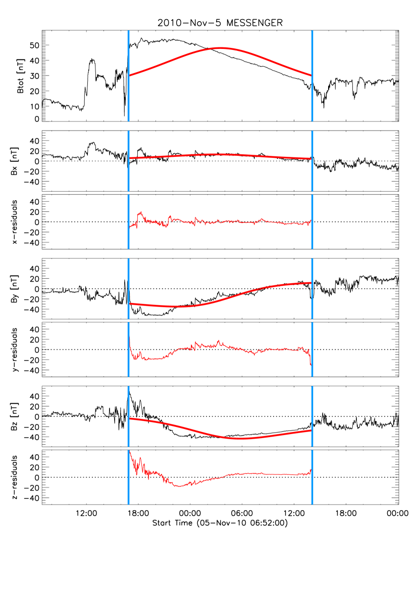
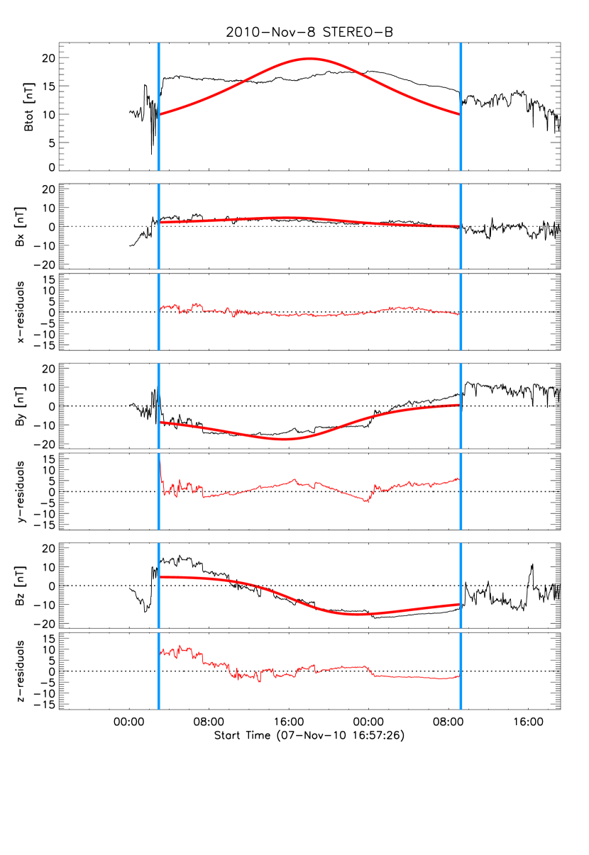
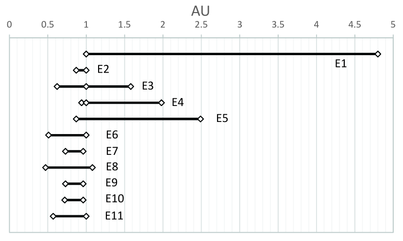
In the following, we analyze 11 events that were observed by at least two radially aligned spacecraft. In particular, we employ data measured by MESSENGER (MES), Venus Express (VEX), Helios 1 and 2 (H1, H2), Interplanetary Monitoring Platform-8 (IMP8), Wind, STEREO-A (STA), STEREO-B (STB), Pioneer 11 (P11), Voyager 1 and 2 (V1, V2), and compiled in The Space Physics Data Facility OMNI2 data base providing spacecraft-interspersed, near-Earth solar wind data (http://omniweb.gsfc.nasa.gov/). An example of the measurements by two radially aligned spacecraft is presented in Figure 1. The list of events is displayed in Table 1, where Column 1 gives the data label, Columns 2 and 3 the year and the data sources, and Column 4 the time range (expressed in Day of Year; DOY). In Column 5 the distance range (expressed in AU) covered by the measurements is presented; the measurements stretch from to 4.8 AU. The shortest distance between two spacecraft was in Event 2 (E2; 0.87 – 1.00 AU). It is included in this paper only to illustrate that if two spacecraft are too close, the results regarding the evolutionary behavior can become unreliable. It should be noted that the events E7, E9, and E10 were also measured by relatively closely positioned spacecraft ( AU; see Table 1 and Figure 2). The largest distance range was in Event 1 (1.00 – 4.80 AU). Events E3 and E4 were measured by three spacecraft, where in E4 two of the three spacecraft were quite close ( and 1), which we use to get an independent measure of the uncertainty of data obtained at a given distance. The distance ranges covered by measurements are presented for all events in Figure 2. Events 1 – 5 have already been used in the statistical study by Leitner et al. (2007); the event labels from that study are given in Column 6. Events 2 and 4 were also analyzed by Farrugia et al. (2005) (the event labels from that study are given in Column 6 in brackets) and Event 8 was analyzed by Good et al. (2018) and Amerstorfer et al. (2018).
In all events, the magnetic field vector B was measured by all spacecraft. On the other hand, the plasma measurements, including the flow speed, are not available for the events measured by MES and VEX (Events 6 – 11). For these events we estimated the MC propagation speed indirectly, utilizing the following observational information:
-
•
the time when the CME was at the heliocentric distance of solar radii () and its speed at this location (estimated from coronagraphic measurements provided in the SOHO/LASCO CME catalog; Yashiro et al., 2004);
-
•
the time when the MC arrived to MES or VEX (the heliocentric distance );
-
•
the arrival time and speed of the MC at the spacecraft located at 1 AU (Wind, STA, or STB).
The transit time from to was used to estimate the corresponding mean speed , which was attributed to the half-distance . In the same manner, we estimated the speed at the half-distance . In this way, the MC speed at four heliocentric distances (, , , and ) was obtained. Finally, the four speed–distance data points , , , and , were used to interpolate the value of the MC speed at the location where MES or VEX were located.
The flux-rope magnetic field structure was reconstructed by fitting the in situ magnetic field measurements with the Gold-Hoyle force-free uniform-twist configuration (Gold and Hoyle, 1960, for details see Appendix A; for the fitting procedure see Farrugia et al. 1999 and Wang et al. 2016; for different reconstruction techniques see Al-Haddad et al. 2018; for the observational aspect see Vršnak et al. 1988). This model was chosen since it does not restrict the pitch angle of the field lines at the flux-rope boundary to as is the case of the frequently used Lundquist model (Lundquist, 1950). The fitting provides the magnetic field strength in the MC center, , the latitudinal () and longitudinal () direction of the flux-rope axis ( is ranging from to 90∘, and is defined counterclockwise from positive x-direction, pointing towards the Sun and ranging between 0 and ), the impact parameter, , and the sign of helicity, . The “goodness” of the fit is checked by calculating the root-mean-square difference, , between the observed and modelled magnetic field, and the relative deviation defined by , where is the highest measured value of the magnetic field (for details see Marubashi et al., 2015).
The MC diameter is estimated as:
| (1) |
where is the MC speed, is the MC duration, is the closest distance of the spacecraft to the MC center in the plane of the spacecraft orbit (x-y plane in SE coordinate system) normalized with respect to the MC radius, and is the inclination to the spacecraft-Sun line of the projection of the MC-axis onto the plane defined by the spacecraft-Sun line (x-axis in the SE coordinate system) and the normal to the plane of the spacecraft orbit (z-axis in the SE system). Derivation of Equation (1) is presented in https://doi.org/10.6084/m9.figshare.7599104.v1. We also estimated applying the expression used by Leitner et al. (2007), and we found no significant differences in results obtained by these two procedures. The fitting results, combined with the estimated values of , are finally used to calculate the axial magnetic fluxes, , and the axial electric currents, (for details see Appendix A).
Since the estimate of the flux rope extent in the measured magnetic field data is based on subjective judgement, for each event we performed three independent fittings based on three independent estimates of the beginning and end of the flux rope signature in the in situ data. In this way we obtained three different data sets, in the following denoted as “n” (narrow), “b” (best), and “w” (wide), providing an assessment of the uncertainties caused by the subjective estimate of the flux rope extent.
In Table 2 we display the outcome of the fitting for the b-option of the extent of flux ropes (other options will be considered only in graphs and in estimates of uncertainties of various parameters, like flux rope diameter, central magnetic field strength, axial magnetic flux, axial current, etc.). The event label is given in Column 1, which is followed by the basic MC parameters: heliocentric distance, velocity, duration, and peak magnetic field (Columns 2, 3, 4, and 5, respectively). In Columns 6 – 11 the results of the fitting are displayed: the latitudinal () and longitudinal () direction of the flux-rope axis (Columns 6 and 7), the impact parameter normalized with respect to the flux-rope radius (Column 8), the MC diameter (Column 9), the magnetic field strength at the MC center (Column 10), and the sign of helicity (Column 11). In Columns 12 and 13 we present the and values, respectively.
3 Results and Interpretation
3.1 Basic Concepts Considered in the Analysis
In the absence of reconnection, the magnetic flux encircled by the erupting flux rope has to be conserved. Approximating the flux-rope by a simple line-current loop, this flux can be expressed as , where is the self-inductance of the current loop and is the electric current (cf., Batygin and Toptygin, 1962, for the meaning of the inductance in MHD, see e.g., Garren and Chen 1994, or Žic et al. 2007). Since the inductance is proportional to the size of the current loop (, where is the circumference of the current loop (Jackson, 1998, p. 218), the electric current must decrease in the course of the eruption, . Thus, also the relationship must be approximately valid (for the relationship see Appendix B). Note that this is valid not only in the idealized approximation of the line-current loop, but also in the case of a flux rope of finite radius that is not constant along its axis. However, in some specific, quite realistic situations, this very basic physical concept might not be applicable, e.g., when a certain set of field lines twists along a part of the flux rope, but then leaves the flux rope, becoming a set of “open” field lines.
Bearing in mind that the electric current flows through a loop of finite thickness (flux rope), the total inductance is a sum of the “external” and “internal” contribution. The external inductance can be expressed in the “semi-toroidal” approximation (Chen, 1989; Garren and Chen, 1994; Žic et al., 2007) as , where is the permeability, is the length of the flux rope, and is the torus aspect ratio, i.e., the ratio of the major and minor radius of the torus. The internal inductance can be expressed as , where is a constant that depends on the radial profile of the electric current density (for details see Žic et al., 2007, and references therein). Thus, in the absence of magnetic reconnection, again we get that the current has to decrease as . Since both and have to be conserved, also the ratio has to be constant, i.e, the rope should expand self-similarly, (for details see, e.g., Vršnak, 2008, and references therein; for a more rigorous treatment see Osherovich et al., 1993). Thus, under these assumptions, and using the relationships presented in Appendix A and B, the following dependencies are expected: , , , and In this respect, let us note that statistical studies by Kumar and Rust (1996); Bothmer and Schwenn (1998); Liu et al. (2005); Wang et al. (2005); Leitner et al. (2007); Gulisano et al. (2010, 2012) illustrate the appropriateness of the power law presentation of the dependencies of MC parameters on the heliocentric distance.
3.2 Results
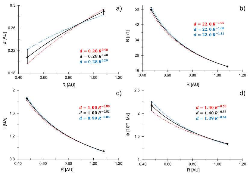
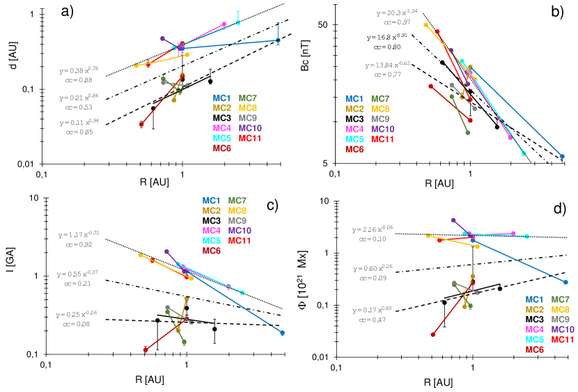
As an example of the individual-event results, we show in Figure 3 the estimated values of the MC diameter , central magnetic field , axial electric current , and axial magnetic flux for E8. As previously mentioned, results for three fitting options (b, n, w) are presented. The data points are connected with the corresponding power-law dependencies, following the arguments explained in Section 3.1. To estimate the ambiguities related to the different fitting options, in addition to the power-law dependency based on the b-fit option (black line), we present in each graph also the power-law connecting the lowest value obtained for the inner spacecraft with the highest value at the outermost spacecraft (red dotted line), as well as the power-law connecting the highest value obtained for the inner spacecraft with the lowest value at the outermost spacecraft (blue dotted line). The power-law coefficients corresponding to the latter two power-law options are presented in Tables 3 and 4 as the superscripts and subscripts on the b-option value.
In Figure 4 results for all events under study are shown together in log-log space, where the power-law dependencies (, , , and are represented by straight lines. Here , , , and correspond to the MC diameter, central magnetic field, axial current, and axial magnetic flux at 1 AU, expressed in AU, nT, GA (= A), Mx, respectively. In the events where there are three data points, we applied a least-squares power-law fit. The power-law coefficients are presented in Tables 3 and 4, for each event individually. In addition to the power-law relations, in Tables 3 and 4, also the linear-dependency coefficients are shown, in the analogous way as for the power-law option.
3.2.1 Diameter and Magnetic Field Strength
In the case of relationship shown in Figure 4a, the least-square power-law fit for the complete data set (dash-dotted line) reads , with the correlation coefficient of and the F-test confidence level of %. However, the distribution of data points indicates that our sample consists of two statistically different subsets, one having larger dimensions, and one having significantly smaller dimensions. We checked this hypothesis by using the t-test and we found that the subsets indeed represent two statistically different populations at %. Consequently, it is worth performing independent fits for the two subsets — the separate power law fits read with (dotted line) and with (dashed line), respectively. The obtained dependencies indicate that both subsets, as well as the overall fit for the whole sample show a statistical tendency broadly compatible with the self-similar expansion, i.e., that the power-law exponent is .
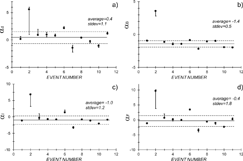
On the other hand, inspecting the values of the power-law slopes for individual events, presented in the fifth column of Table 3 (shown also in Figure 5a), one finds a large scatter, ranging from (contraction) up to 2.19 (strong expansion). Note that in the following, we neglect event E2 since the two spacecraft were too close (0.13 AU; see Table 1 and Figure 2) to provide a reliable result on its heliospheric evolution. It should be noted also that the three events showing a contraction, i.e., (E7, E9, E10) were measured by relatively closely-positioned spacecraft ( AU; see Table 1 and Figure 2). According to Table 3 only four events (E3, E4, E5, and E11) show , i.e., the values that are compatible with a self-similar expansion. The large scatter of individual values results also in a large uncertainty in the average value shown at the bottom of Table 3, . However, if the events E7, E9, and E10 (spacecraft separated by AU) are excluded, one finds that the remaining seven-event subsample shows , which is consistent with self-similar expansion.
In Figure 4b the dependence is presented in an analogous way as in Figure 4a for the relationship. The least-square power-law for the complete data set (dash-dotted line) reads , with a correlation coefficient of and the F-test confidence level of %. We performed also separate fits for the two subsets like in the case of the dependence, giving with and with , for the larger and smaller MC-dimension subsets, respectively. However, in this case the subsets are not significantly different, since the F-test shows %, implying that the magnetic field strength in the considered sample does not depend significantly on the MC size. The obtained power-law slopes in any of these options are significantly different from that expected for the case of the so called isotropic self-similar expansion, meaning in addition to (for a definition of “isotropic self-similar expansion” see e.g., Démoulin and Dasso (2009) and references therein; hereafter we will simplify it to “self-similar expansion”).
Inspecting the values of the power-law slopes for individual events, presented in the last column of Table 3 and in Figure 5b, one finds again a relatively large scatter of values, yet all (except the “unreliable” E2) showing a decrease of (). The values of range from to , with an average value of . Inspecting in detail the last column of Table 3, one finds that only the events E7, E10, and E11 are compatible with a self-similar expansion (). In all other events one finds , mostly in the range of , meaning that the magnetic field weakens at a significantly lower rate than expected in the case of self-similar expansion, .
We end this subsection by comparing in parallel the change of the MC diameters and their magnetic field (Table 5). Assuming a circular cross section of the flux rope and the magnetic flux conservation, one would expect the relationship , since the cross-sectional area in such a case is , i.e., , implying . The values of are listed in Column 2 of Table 5 and are compared with (Column 3). In Column 4, the quantity is displayed, represented also as in the form of percentiles (Column 5). In Column 6 we present the ratio , which is expected to be in the case of self-similar expansion.
Inspecting Table 5 one finds that in most events there is a large difference between and , i.e. in most events the relationship is not satisfied. This implies that some other effects play a significant role in the MC evolution, like e.g., magnetic reconnection that changes the magnetic flux of the rope, or a deformation of the shape of the flux-rope cross section. Yet, we note that the average value of the ratio (see the last two rows of the last column of Table 5) is broadly compatible with the value expected for the case of self-similar expansion.
3.2.2 Inferred Electric Current and Magnetic Flux
In Figure 4c the behavior of the inferred axial electric current is shown for all events plotted together, including the power-law least square fits analogous to that applied in Figures 4a and 4b for the and dependencies. The fit for the complete data set reads , where the electric current is expressed in GA (the same applies to Table 4). The corresponding correlation coefficient is . Thus, the found dependence shows a statistical tendency of decreasing , but at a significantly lower rate than expected for self-similar expansion (). The separate fits for the two subsets corresponding to those in the dependence read with and with , respectively. Thus, in a statistical sense, the subset of MCs with larger diameter show clearly a decreasing trend of the axial current, whereas smaller MCs apparently show no change of current.
However, inspecting the individual-event power-law exponents , displayed in Table 4 (shown also in Figure 5c), one finds that all events, except the event E6 and the “unreliable” event E2, show a decrease of the axial current. Note that approximately half of events show close to that expected for the self-similar expansion. The average value shown at the bottom of Table 4, , obtained by omitting the E2 outlier (see Figure 5c), is compatible with that expected for the case of the self-similar expansion. If we also omit the extreme-value events E6 and E7 (see Figure 5c), we obtain , i.e., again compatible with self-similar expansion, but now with a somewhat lower standard deviation.
The behavior of the inferred axial magnetic flux is shown in Figure 4d for all events plotted together, including the power-law least square fits analogous to that applied in Figure 4c for the dependence. The fit for complete data set reads , where the magnetic flux is expressed in units of Mx (the same applies to Table 4). The corresponding correlation coefficient is only . Thus, bearing in mind a large uncertainty of the power-law exponent and very low correlation coefficient, as well as the fact that the flux rope interval chosen at one location may not match entirely the interval chosen at the other, the axial magnetic flux can be considered as constant. The separate fits for the same two subsets read with and with , i.e., the former one is compatible with , whereas the latter one indicates a weak, yet statistically insignificant, increasing trend of .
On the other hand, the average value , presented at the bottom row of Table 4, is broadly compatible with . If we exclude E2 and the extreme-value events E6 and E7 (see Figure 5c), we find , again being broadly compatible with
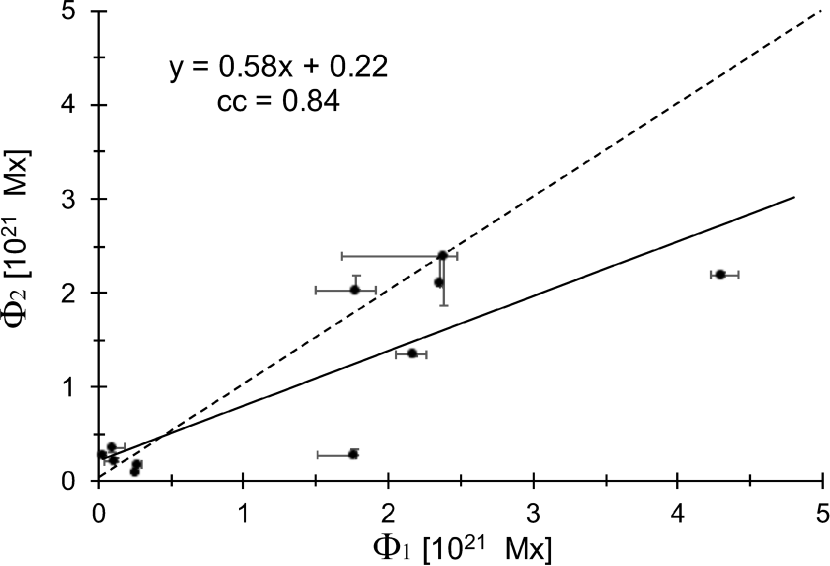
In Figure 6 the effect of decreasing axial magnetic flux is emphasized by showing for each event the flux inferred from the measurements at the farthermost spacecraft, , versus the flux obtained for the spacecraft closest to the Sun, . The graph shows that data points tend to be below the line, i.e., in most of events the value of is smaller than . The linear least square fit to the data points reads , with a correlation coefficient of . A linear fit fixed at the origin, gives , with . Note that the correlation is dominated by events with large values of ( Mx), where all events show either (E1, E8, E10) or (E4, E5, E11). For the six events with large , the average relative decrease amounts to %, consistent with the mentioned fit .
4 Discussion
The relationships expected for self-similar expansion of the cylindrical force-free flux rope (Section 3.1) are not fully consistent with the observations presented in Section 3.2. Even taking into account only the measurements where the spacecraft were radially separated by more than 0.4 AU, where the statistical trend is compatible with the self-similar expansion form , individual events show a great variety of behaviors, from very weak to very strong expansion (Table 3). According to Table 3 only four events (E3, E4, E5, and E11) show .
The behavior of the magnetic field strength shows an even more significant deviation from that expected for the self-similar expansion, even in the statistical sense. The overall fit through whole data set (Figure 4b) shows that the rate at which decreases is characterized by , which is significantly lower than that for self-similar expansion (). Accordingly, most of the events individually show a similar behavior, resulting in a mean value of . Table 3 shows that only three events (E7, E10, and E11) are compatible with a self-similar expansion (). Finally, Figure 6 indicates that in the statistical sense, the axial magnetic flux decreases with distance. Thus, the analyzed set of events might indicate that there is a significant reconnection reducing the MC size and the magnetic flux by “peeling-off” the outer layers of the rope (Dasso et al., 2006, 2007; Gosling et al., 2007; Möstl et al., 2008; Ruffenach et al., 2012), or more likely, that the assumption of a circular cross section is, at least in a fraction of events, not valid. In this respect, it should be emphasized that the imperfection of existing models is the leading cause of uncertainty in reaching a definitive conclusions; note that the flux erosion as inferred here and in previous papers, is based on usage of very simplified models, so the validity of such results remains questionable.
4.1 Nonuniform Flux-Rope Expansion
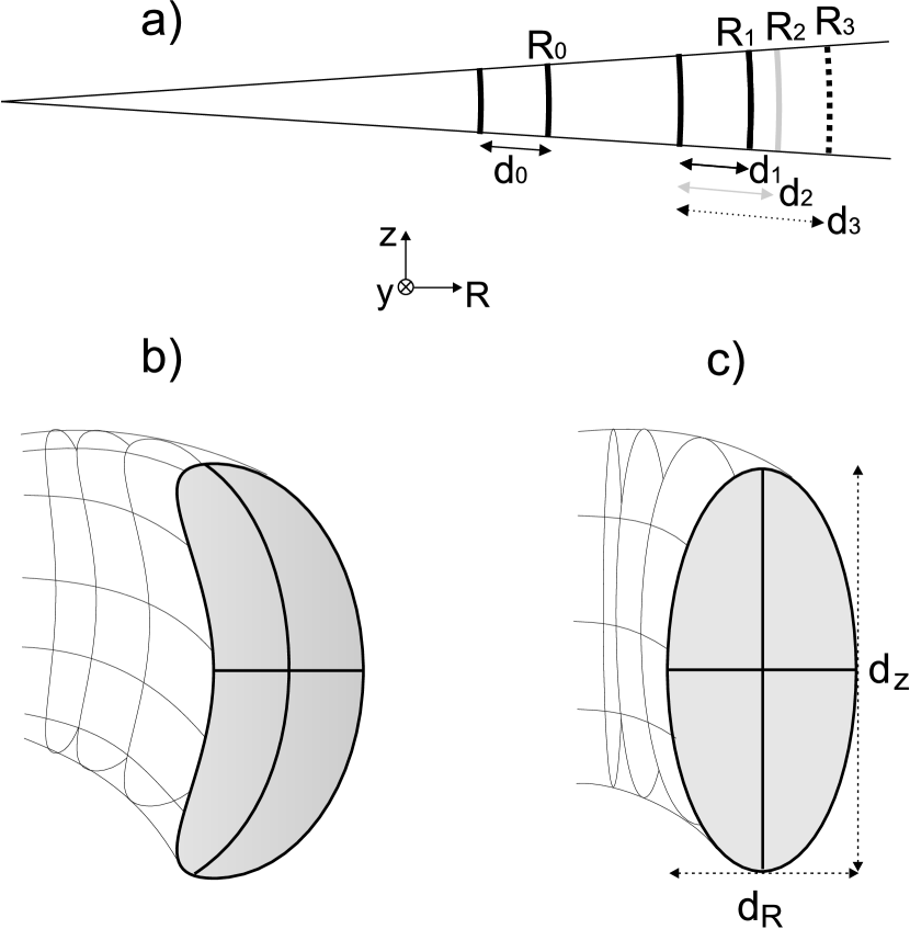
Let us first consider the effects of a “nonuniform” expansion, schematically drawn in Figure 7a. The axial magnetic field is oriented in -direction. In -direction the considered element expands in a self-similar manner, whereas for the radial expansion three options are taken into account. Initially, the element has a thickness , with the frontal edge set at a heliocentric distance . In the course of time, the element propagates to a larger distance, , and attains a thickness (, 2, 3).
The expansion depicted by the bold-black frontal edge at the distance represents the option where the element does not change its thickness, i.e., , so the cross-section area behaves as . Note that in such a case there should be no velocity gradients within a MC (), i.e., the MC speed is fully adjusted to the ambient solar wind speed. Bearing in mind the flux conservation, the magnetic field in the element would decrease as , i.e., much slower than in the case of the self-similar expansion where it is characterized by . Such a behavior is found (see Table 3) in events E1, E3, E6, E8, and E9, where all but E3 and E6 show only a very weak or no expansion.
The self-similar expansion is depicted in Figure 7a by the bold-dotted line at , where . Here, the expansion should be characterized by and . The only event that satisfies both conditions is E11. The events E7 and E10 show , however in these events corresponds to the MC contraction (yet, as mentioned in Section 3.2.1, the values of are based on measurements by two relatively closely located spacecraft). In the events E3 and E4 we found , however the decrease of is much weaker than in the case of self-similar expansion.
The expansion denoted by the bold-gray line at represents an intermediate case, where . In this option, the field decreases as , where , just like it was found (in the statistical sense) from the observations in Section 3.2.1. Such behavior is found in E4 and E5.
Based on numerical simulations of the flux-rope propagation it can be expected that the expanding flux rope has the outward-convex shape depicted in Figure 7b (“pancaking effect”) due to pressure gradients and/or the MHD “aerodynamic” drag (see, e.g., Cargill et al., 1994, 1996, 2000; Riley and Crooker, 2004; Owens et al., 2006). In the interest of simplicity, let us approximate such a structure by an elliptical cross-section, as drawn in Figure 7c (for the magnetic field configuration in such a rope see, e.g., Vandas and Odstrcil, 2004; Riley et al., 2004). In particular, we assume that the expansion in the direction perpendicular to the plane of the flux rope axis, which is set in the - plane is proportional to . This means, that for the thickness in -direction is valid, i.e., , meaning that the major axis of the cross-sectional ellipse expands in a self-similar manner. For the thickness in the -direction we allow that the ratio is a function of distance, in particular, . In that case the cross-sectional area behaves as , where represents the MC heliocentric angular width in the -direction. Under the described approximations and in the absence of reconnection, the magnetic field should decrease as , i.e., the relation should be valid.
In Column 7 of Table 5 the values of are listed, and in Column 8 we display the ratio . One finds that in the E1, E4, E5, E8, E9, and E11, differs from within 30 %. Considering the measurement uncertainties, this is consistent with the assumption that the expansion in -direction is confined to , i.e., the measurements could be interpreted by nonuniform expansion without including some additional effects.
On the other hand, in the remaining four events (again excluding E2), E3, E6, E7, and E10, the difference of and is much larger and the magnetic field decrease cannot be explained solely by the expansion. Consequently, such a decrease of the magnetic field indicates that either the magnetic flux was significantly reduced by reconnection, or these MCs significantly “over-expanded” in -direction, i.e., . Note that the latter effect is found in numerical simulations presented by Riley and Crooker (2004). However, note that E7 and E10 were measured by two relatively closely located spacecraft, so here the results are quite uncertain, and the difference might be only due to errors in measurements. Also note that E3, E6, and E7 were events of low magnetic flux, so reconnection can play a more important role than in the case of large-flux events.
4.2 Magnetic Reconnection
In Figure 8, reconnection of the helical field of the rope and the external field is sketched. In the following it is assumed that the reconnection takes place at the leading edge of the MC over the length , and we take approximately , where is the angular extent of the flux rope in the plane of its axis (- plane in Figures 7 and 8). A local reconnection rate is determined by the product , where is the inflow speed of the magnetic field into the diffusion region (note that value of has to be equal on the opposite sides of the diffusion region). Thus, the rate at which the magnetic flux is reconnected over the length equals to , where the values of , , and depend on the heliocentric distance.
Under these assumptions, the total reconnected flux in the time interval from to amounts to:
| (2) |
which can be expressed by integrating over the corresponding heliocentric distance range as:
| (3) |
where we used d = d for the MC propagating at an average speed . In the following, we take that the ambient interplanetary magnetic field decreases approximately as (Vršnak et al., 2004a), i.e., we take . Assuming that the solar wind expands at a constant speed and that the expansion is approximately isotropic, one finds that the density varies as (e.g., Vršnak et al., 2013), so the Alfvén speed should decrease roughly as . Thus, , , and can be expressed as:
| (4) |
where subscript 1 stands for the value at 1 AU, and is expressed in AU. The reconnection inflow speed is a small fraction of the local Alfvén speed , with – 0.1 (e.g., Priest, 1982, and references therein). In such a case, the total flux that is reconnected in the course of the MC propagation from to equals to:
| (5) |
where is expressed in AU, and stands for:
| (6) |
Here, the numerical factor m represents 1 AU, and if the ambient field is expressed in T, Equation (5) provides the results in Wb, which corresponds to Mx. After integrating Equation (5), the total flux reconnected while the MC travels from to reads:
| (7) |
Substituting the values rad, , nT, km s-1, and km s-1, one finds that in the case of fully antiparallel fields of MC and ambient solar wind, the flux reconnected over a distance range from to equals to Wb Mx. This is an order of magnitude lower than estimated in Section 3.2.2, and is consistent with the results presented by Gosling et al. (2005). On the other hand, closer to the Sun, the reconnected flux could be much larger, as inferred also by Ruffenach et al. (2012). For example, for and one gets Mx.
In Table 6 the observed change of the magnetic flux from the first to the last spacecraft measurement (only the decreasing- events are shown) is compared with the reconnection-related change calculated using Equation (11). The ratio of these two values, given in Column 7, shows that the observed flux change is larger than that presumably caused by reconnection. We note that for the calculation of the reconnected flux we used , which is an upper limit for the reconnection rate, so the calculated values represent an upper limit, particularly considering the most favorable case of fully antiparallel field of MC and ambient solar wind. The only event where the observed and calculated changes of the flux coincide is E9, where the initial magnetic flux is very low. We also note that the observed values of do not show any statistically significant dependence on the heliospheric distance that is predicted by Equation (7). These findings imply that reconnection alone cannot explain the inferred magnetic flux changes, since its effect is more than one order of magnitude weaker than required.
Finally, we stress that Equation (7), due to the dependence , indicates that in the case of fast MCs the effect of reconnection is expected to be much weaker than in the case of slow MCs, which is related to shorter time available for reconnection. For example, taking km s-1, and using the set of parameter values rad, , nT, and km s-1, one finds that from to , less than Mx is expected to be reconnected. Since fast MCs are usually characterized by strong magnetic field, implying also a large magnetic flux, in such events the reconnection-related relative decrease of the magnetic flux is probably negligible. On the other hand, in the case of slow MCs, the reconnection can be a significant factor. Taking the same parameters as in the previous example, only now substituting km s-1, one finds that a flux of Mx could be reconnected, implying that low-flux MCs may be entirely “melted” into the background solar wind before reaching the Earth.
Finally, let us also note that reconnection affects not only the magnetic flux of MCs, but also their diameter, since “peeling-off” the outer layers of the flux rope should lead to lowering the expansion rate of MCs. This might at least partly explain the expansion rate characterized by .
4.3 Comparison with Previous Studies, and Accuracy of the Results
In the following, the results presented in Section 3.2 are compared with the results of previous studies on the heliospheric evolution of the MC size and magnetic field. First we give an overview of the statistical aspects, and then we focus on the evolution of individual events.
The slope of the “overall” power-law fit to all data shown in Figure 4a reads . This value falls into the range found in the statistical studies by Kumar and Rust (1996), Bothmer and Schwenn (1998), Liu et al. (2005), Wang et al. (2005), Leitner et al. (2007), Gulisano et al. (2010), and Gulisano et al. (2012), where is found in the range from (Gulisano et al., 2012) to (Kumar and Rust, 1996). On the other hand, the mean value of the slopes obtained for individual events, (Table 3), is considerably lower than most of previously reported values. However, omitting the events E7, E9, and E10 (spacecraft separated by AU, showing MC contraction), the remaining seven-event subsample gives , which is consistent with self-similar expansion.
In this respect, it should be noted that all of the previously mentioned studies show large variety of values, the differences generally being larger than the reported error estimates. Moreover, as demonstrated in Section 3.2.1, the statistical results based on a sample of single spacecraft measurements could be misleading since the outcome depends on the distribution of data points over a given distance range, particularly bearing in mind the effect of weakening of the expansion with increasing heliocentric distance (e.g., Osherovich et al., 1993; Liu et al., 2005; Wang et al., 2005; Leitner et al., 2007; Gulisano et al., 2012).
In any case, we emphasize that most of the mentioned studies show the dependence with , i.e., reveal a deviation from self-similar expansion. We also note that the back-extrapolation of both the power-law and the linear relationships lead to far too large MC sizes in the solar vicinity. From this one can infer that the MC expansion is much more pronounced at small heliocentric distances, consistent with the results presented by Leitner et al. (2007) and Wang et al. (2005).
When the evolution of individual events is considered, our results could be compared with only a few case studies. Bothmer and Schwenn (1998) presented as example a MC observed by Helios 1 at 0.9 AU and by Voyager 1/2 at 2.6 AU, roughly doubling its thickness over this distance range. This would correspond to , which is comparable to our events E5 and E8. A similar expansion rate was found by Savani et al. (2009), who analyzed the Heliospheric Imager remote observations of one circularly-shaped CME.
Nieves-Chinchilla et al. (2012) performed a very detailed study of the evolution of a MC recorded by the MES at AU and by the Wind spacecraft at 1 AU. They applied several magnetic reconstruction techniques and various assumptions on the MC boundaries, to demonstrate how much the results depend on the methodology applied. The differences turned out to be very large in determining the MC diameter, resulting in very different expansion rates — from the data presented in the paper one finds cases from shrinking with , up to expansion with . The expansion, , was also traced from the HI data in the range AU, which helped to resolve this ambiguity, giving the expansion rate in the direction of motion consistent with that found statistically by Bothmer and Schwenn (1998). Note that the results displayed in Table 3 show a similar spread of , ranging from to .
From the results presented in Table 3 one finds power-law slopes ranging from to . This is consistent with the power-law slopes found by Kumar and Rust (1996), Liu et al. (2005), Wang et al. (2005), Leitner et al. (2007), Gulisano et al. (2010), and Gulisano et al. (2012), that range from (Leitner et al., 2007) to (Gulisano et al., 2010), again showing a large scatter of values.
The “overall” power-law fit to all data points shown in Figure 4b has a slope of , whereas the mean value of the slopes obtained for individual events gives (Table 3). The former value is close to that found by Leitner et al. (2007), whereas the latter value is close to obtained by Du et al. (2007). Inspecting the dependence of the slopes on the heliocentric distance in the mentioned papers, one finds that the decrease of the magnetic field is faster closer to the Sun than at large distances ( in the range 0.3 – 1 AU, versus to in the range 1.4 – 5.4 AU), which is consistent with weakening of the expansion with increasing distance.
Osherovich et al. (1993) studied theoretically a self-similar expansion of MCs and compared the results with the in situ measurements of a MC recorded by Helios 2 at 1 AU and Voyager 2 at 2 AU. It was shown that over this distance range the central magnetic field decreased by a factor of four, corresponding to , i.e., being consistent with the self-similar expansion.
Nieves-Chinchilla et al. (2013), studied an ICME identified in the MES data (located at AU), which was also recorded at the STB spacecraft that was aligned with MES at the distance of AU. Although the evolution of the internal magnetic field structure was not analyzed in detail, from the data presented in the paper it can be inferred that the thickness of the MC contained in the ICME was increasing at the rate . The measured (i.e., not reconstructed) magnetic field was decreasing at the rate , thus also showing a behavior that is inconsistent with self-similar expansion.
Good et al. (2015) analyzed a MC observed by MES located at 0.44 AU and later by the STB spacecraft at 1.09 AU in early November 2011. The applied force-free fitting showed that the MC size was increasing at the rate , whereas the magnetic field decrease was characterized by . The analysis showed that the axial magnetic flux was conserved, i.e. no significant erosion took place between 0.44 and 1.09 AU.
Du et al. (2007) studied the evolution of the magnetic flux and helicity of the MC recorded by ACE at Earth on 4-6 March 1998 and later by Ulysses at 5.4 AU. Applying the Grad-Shafranov reconstruction technique, they found that the inferred value of the axial flux decreased by an order of magnitude. From the presented values of the peak axial magnetic field component one finds that it decreased at a rate of , the size increase was characterized by , whereas the axial-flux decrease is characterized by to . These rates are in the range of the values presented in Table 3.
Mulligan et al. (2001) studied the evolution of the MC associated with the “Bastille-day flare” employing the in situ data from the ACE and NEAR spacecraft that were located at and AU. They found , which is very close to the mean value displayed in Table 3 (). It was also inferred that the magnetic flux increases at a rate of .
The discussion presented in the previous paragraphs shows that the conclusions on the evolution of MCs can be quite ambiguous since the empirical results depend on a number of factors. For example, the outcome of the magnetic field reconstruction strongly depends on the level of complexity of the true magnetic structure of a given MC and the trajectory of the spacecraft. Furthermore, different reconstruction methods give different results (see, e.g., Dasso et al., 2006). Finally, the outcome to a certain degree depends on the interpretation of the measurements, e.g., the estimate of the MC boundaries, which is subjective and often differs from author to author.
Regarding the errors and reliability of the results, it should be noted that it is quite difficult to estimate the accuracy of the results in the case when the analysis is based on only two spacecraft. In this respect, our study provides a certain insight into the errors since in the events E3 and E4 measurements from three different in situ observatories are available (see Table 1 and Figure 2). In E4 the first two spacecraft were located at similar heliocentric distances, 0.94 and 1 AU (Figure 2), and the reconstruction resulted in very similar outcome (see measurements 4a and 4b in Table 2 and check E4 Figure 4).
On the other hand, it should be noted that the situation was quite different in the case of E2, where measurements were also performed at two relatively closely spaced spacecraft (0.87 and 1 AU). In this event the outcome for the two spacecraft were quite different, particularly in the case of the diameter and the reconstructed central magnetic field (see measurements 2a and 2b in Table 2 and check E2 in Figure 4). Similarly, in E3, where the three spacecraft were located at = 0.62, 1, and 1.58 AU, the evolution of the estimated MC velocities shows a considerable scatter ( = 289, 462, and 376 km s-1, respectively), which results also in a considerable scatter in the diameter evolution ( = 0.056, 1.35, and 0.128 AU, respectively; see measurements 3a, 3b, and 3c in Table 2 and check E3 in Figure 4). On the other hand, the values of show a smooth decay with . However, due to the scatter in the dependency, the inferred dependencies and also show a significant scatter.
5 Conclusions
We presented a study of the evolution of eleven MCs based on the in situ measurements by at least two radially aligned spacecraft. The analysis has shown that reliable results can be obtained only if the spacecraft separation is AU. It is also shown that there is a large difference between the behavior of individual events and the overall statistical trends. Thus, overall fits, like those presented by Kumar and Rust (1996), Bothmer and Schwenn (1998), Liu et al. (2005), Wang et al. (2005), Leitner et al. (2007), Gulisano et al. (2010, 2012) should be taken with some caution, since they can lead to wrong physical interpretations of individual events. Bearing in mind these two facts, the results of our study can be summarized as follows.
-
•
In the statistical sense MCs in the sample show an expansion compatible with self-similar expansion (). However, individual events show a large scatter of expansion rates, ranging from very weak to very strong expansion; only four events show an expansion rate compatible with self-similar expansion. The results indicate that the expansion has to be much stronger when MCs are still close to the Sun.
-
•
The magnetic field shows a large deviation from the behavior expected for the case of a self-similar expansion. In the statistical sense, as well as in most of individual events, the inferred magnetic field decreases much slower than expected. Only three events show a behavior compatible with self-similar expansion.
-
•
The presented analysis indicates that there is also a discrepancy between the magnetic field decrease and the increase of the MC size, suggesting that magnetic reconnection and the “pancaking effect” might play a significant role in the MC evolution. However, bearing in mind the usage of very simplified models, as well as the fact that the reconstruction of the magnetic configuration is based on single-point time series, this indication has to be taken with caution.
-
•
Individually, about half of the events show the decay of the electric current as expected in the case of self-similar expansion, which is also reflected in the mean value of the decay rate.
-
•
In the statistical sense, the inferred axial magnetic flux is broadly consistent with staying constant during the MC evolution. However, events characterized by large magnetic flux show a clear tendency of decreasing flux.
The presented analysis shows some significant deviations from the behavior expected for self-similar evolution of MCs. In some events the diameter increases at a rate much lower than , which might be explained by gradual adjustment of the MC dynamics to the ambient solar-wind flow. Generally, there is a tendency that ejections that are faster than the solar wind decelerate, whereas those that are slower accelerate during their interplanetary propagation (e.g., Gopalswamy et al., 2000), as a consequence of the “magnetohydrodynamic drag” (e.g., Cargill, 2004; Vršnak et al., 2008, 2013, and references therein). Due to the same effect one would expect that the broadening of the MC body gradually weakens, until eventually all elements attain the speed of the ambient solar wind. Since the overall solar-wind flow is characterized by a constant velocity, this implies that all elements of the MC should attain the same speed. Consequently, there should be no change of the MC diameter at large heliocentric distances. It should be noted that the absence of velocity gradients, and the related disappearance of the frontal sheath region, would make the identification of ICMEs in the in situ data considerably more difficult.
Qualitatively, the reduced expansion rate is consistent with a slower decrease of the MC magnetic field than is expected in the case of self-similar expansion. Yet, there is a considerable discrepancy in quantitative terms in several events, where the decay of the magnetic field is not consistent with the expansion rates.
An apparently plausible way to explain the mentioned discrepancies, is to presume that they are due to magnetic reconnection occurring between the internal MC field and the ambient interplanetary field (Dasso et al., 2006, 2007; Gosling et al., 2007; Möstl et al., 2008; Ruffenach et al., 2012). The effect of reconnection is to peel off outer layers of the flux rope, thus decreasing MC thickness and reducing its magnetic flux, and consequently, affecting also the axial electric current. However, the presented order of magnitude considerations show that the effect of magnetic reconnection is at least one order of magnitude too weak to explain the noted discrepancies. From this, it can be concluded that the only viable effect that can provide an explanation for the observed MC evolutionary characteristics is the “pancaking effect” (see, e.g., Cargill et al., 1994, 1996, 2000; Mulligan et al., 2001; Mulligan and Russell, 2001; Riley and Crooker, 2004; Owens et al., 2006), i.e., the effect that leads to a deformation of a flux-rope that initially has a circular cross section, expanding much more in the direction perpendicular to the plane of the flux-rope axis than in radial direction (for a discussion see Möstl et al., 2009, and references therein). In cases where the “pancaking effect” is very pronounced, the standard methods of the magnetic field reconstruction are not appropriate, leading to internal inconsistencies of the results, as demonstrated, e.g., numerically by Riley and Crooker (2004) and observationally by Mulligan and Russell (2001). In the latter paper the effect of MC “flattening” was inferred by studying data from two spacecraft (PVO and ISEE 3), separated longitudinally by 0.21 AU and radially by 0.02 AU. The analysis showed that fitting a non-cylindrical flux rope model to the observational data from both spacecraft simultaneously, results in a stretched rope having almost twice as much magnetic flux than estimated by the independent cylindrically symmetric fit at PVO and five times larger than the flux calculated using the ISEE 3 data. Thus, a deviation from the cylindrically symmetric approximation is the most probable explanation for the apparent flux decrease found in the events under study.
Appendix A Gold-Hoyle Configuration
In the force-free uniform-twist Gold-Hoyle configuration (Gold and Hoyle, 1960, hereafter GHC) the axial and poloidal magnetic field components are defined as:
| (A1) |
| (A2) |
respectively, where is the radial coordinate normalized to the flux-rope minor radius , is the magnetic field at the rope axis, and is field-line twist per unit length:
| (A3) |
where is end-to-end twist (”total twist”), is the end-to-end length of the rope, and is the number of turns a field line makes from one end of the flux rope to another and we abbreviated . In the GHC and do not depend on , meaning by definition that it represents a “uniform twist” configuration. Note that both and are constant, due to the photospheric line-tying condition. The parameter can be also expressed as:
| (A4) |
where is the pitch angle of the field line (note that in the uniform twist case, ). Thus, represents the tangent of the field-line pitch angle at the flux-rope surface, or equivalently, the ratio at the flux-rope surface.
Integrating over the flux-rope cross section, one finds the total longitudinal flux of the GHC:
| (A5) |
i.e.,
| (A6) |
where , and .
On the other hand, employing the relation , one finds the total axial current of the GHC:
| (A7) |
where From this one finds:
| (A8) |
where we have taken into account (see Section 3.1), i.e., . The constant can be expressed as , where and are the flux-rope length and current for the MC at 1 AU.
Equating Eq. (A6) and Eq. (A8), one finds:
| (A9) |
which can be satisfied only if , since Bearing this in mind, Eq. (A3) and Eq. (A6) imply and , respectively, whereas implies , as well as . To summarize, the flux-rope thickness, , the axial current, , the central magnetic field, , and the field-line pitch angle, can be expressed as:
| (A10) |
with , , and , where subscript “1” denotes values at 1 AU. The last relationship in Eq. (A10) implies also . Representing the overall shape of MC by a semi-toroidal flux rope, or some other shape satisfying (see Appendix B), the relationships defined in Eq.(A10) can be rewritten as:
| (A11) |
Such a behavior is usually qualified as “self-similar expansion”.
Appendix B Flux-Rope Length – Distance Relationship
In the following, the relationship between the flux-rope axis length, , and the heliocentric distance, , is considered for different geometries: 1) circular; 2) cone-A; 3) cone-B; 4) cone-C, which are shown in Figure 9. It should be mentioned that the shapes cone-A and cone-B are not really appropriate to represent the flux-rope axis since they have “knees” at the points where the two radial lines connect to the circular frontal arc (in cone-A it is an arc concentric with the solar surface, and in cone-B it is a semi-circle).
For the mentioned flux-rope axis shapes the relationships read:
| (B1) |
| (B2) |
| (B3) |
| (B4) |
respectively, where is the solar radius, and is the angle between the flux-rope axis legs. Note that Equations (A1) – (A4) can be written in the form , where and are constants (, , , , and , , respectively.
In Figure 10 the dependencies defined by Equations (A1) – (A4) are displayed. The main graph represents the range 0.01 AU 0.2 AU (i.e., 2 – 40 ), where the deviations from the are significant. At heliocentric distances beyond 20 the deviation from is negligible (see the graph in the inset of Figure 10). For example, if the functions defined by Equations (A1) – (A4) are fitted by the power-law () over a distance range 0.6 – 2.5 that is covered by measurements employed in this paper, the power-law slopes are 1.0042, 1.0013, 1.0015, and 0.0016, respectively, i.e., the deviation from is on the order of 0.1%. The difference becomes 1 % if the considered distance range is extended down to 10 .
| event | time range | distance | |||
|---|---|---|---|---|---|
| label | year | data source | (DOY) | range (AU) | label* |
| 1 | 1974 | IMP8, P11 | 285-299 | 1.00-4.80 | 1 |
| 2 | 1975 | H1, IMP8 | 321-321 | 0.87-1.00 | 2 (2) |
| 3 | 1977 | H2, IMP8, V1 | 328-333 | 0.62-1.58 | 4 |
| 4 | 1978 | H2, OMNI, V1 | 004-008 | 0.94-1.98 | 5 (1) |
| 5 | 1978 | H1, V2 | 060-069 | 0.87-2.49 | 6 |
| 6 | 2009 | MES, Wind | 069-071 | 0.51-1.00 | – |
| 7 | 2009 | VEX, STA | 191-193 | 0.73-0.96 | – |
| 8 | 2010 | MES, STB | 309-313 | 0.47-1.08 | – |
| 9 | 2011 | VEX, STB | 359-361 | 0.73-1.08 | – |
| 10 | 2013 | VEX, STA | 008-010 | 0.72-0.96 | – |
| 11 | 2013 | MES, Wind | 192-195 | 0.57-1.00 | – |
| event | ||||||||||||
|---|---|---|---|---|---|---|---|---|---|---|---|---|
| [AU] | [km s-1] | [h] | [nT] | [deg] | [deg] | [AU] | [nT] | |||||
| 1a | 1 | 449 | 31.9 | 18.7 | 97.2 | -49.1 | 0.20 | 0.351 | 24.8 | -1 | 5.81 | 0.31 |
| 1b | 4.8 | 418 | 45.0 | 5.7 | 95.4 | -44.0 | 0.04 | 0.452 | 5.6 | -1 | 3.03 | 0.53 |
| 2a | 0.87 | 330 | 9.0 | 14.4 | 84.1 | -11.1 | -0.12 | 0.071 | 15.0 | -1 | 2.99 | 0.21 |
| 2b | 1 | 361 | 17.4 | 15.4 | 83.9 | -28.0 | -0.26 | 0.156 | 24.7 | -1 | 2.69 | 0.18 |
| 3a | 0.62 | 289 | 9.3 | 36.8 | 121.9 | 12.4 | -0.04 | 0.056 | 26.7 | -1 | 13.28 | 0.36 |
| 3b | 1 | 462 | 18.6 | 18.1 | 40.8 | -2.9 | -0.01 | 0.135 | 16.5 | -1 | 6.61 | 0.37 |
| 3c | 1.58 | 376 | 14.0 | 11.6 | 85.7 | 18.6 | 0.15 | 0.128 | 9.2 | -1 | 3.88 | 0.33 |
| 4a | 0.94 | 526 | 28.5 | 20.9 | 257.7 | 44.3 | 0.20 | 0.363 | 22.8 | 1 | 5.61 | 0.27 |
| 4b | 1 | 581 | 36.0 | 19.9 | 230.1 | 5.1 | 0.02 | 0.387 | 22.5 | 1 | 7.67 | 0.39 |
| 4c | 1.98 | 579 | 52.0 | 10.2 | 260.5 | 45.0 | 0.25 | 0.743 | 7.7 | 1 | 2.80 | 0.28 |
| 5a | 0.87 | 443 | 33.2 | 27.9 | 79.9 | 54.9 | -0.11 | 0.354 | 27.4 | -1 | 7.82 | 0.28 |
| 5b | 2.49 | 469 | 72.0 | 6.0 | 73.0 | 9.2 | 0.00 | 0.779 | 5.9 | -1 | 1.40 | 0.23 |
| 6a | 0.51 | 310 | 4.8 | 20.8 | 62.9 | 43.7 | -0.01 | 0.034 | 18.0 | 1 | 6.22 | 0.30 |
| 6b | 1 | 353 | 17.5 | 15.6 | 91.7 | 79.0 | 0.01 | 0.149 | 10.2 | 1 | 3.71 | 0.24 |
| 7a | 0.73 | 290 | 24.8 | 15.8 | 230.1 | 20.4 | -0.02 | 0.138 | 15.2 | -1 | 4.47 | 0.28 |
| 7b | 0.96 | 315 | 13.7 | 8.5 | 242.7 | 17.3 | 0.11 | 0.094 | 8.3 | -1 | 2.03 | 0.24 |
| 8a | 0.47 | 400 | 21.2 | 54.6 | 88.5 | -60.1 | -0.18 | 0.208 | 49.8 | 1 | 13.27 | 0.24 |
| 8b | 1.08 | 399 | 30.3 | 17.7 | 82.8 | -32.2 | -0.07 | 0.290 | 20.3 | 1 | 4.46 | 0.25 |
| 9a | 0.73 | 550 | 10.6 | 19.7 | 119.1 | -6.8 | -0.03 | 0.123 | 18.4 | 1 | 5.73 | 0.29 |
| 9b | 1.08 | 352 | 14.7 | 15.0 | 117.6 | -13.4 | -0.05 | 0.111 | 12.4 | 1 | 2.36 | 0.16 |
| 10a | 0.72 | 600 | 30.2 | 30.9 | 259.4 | 74.7 | 0.41 | 0.475 | 32.7 | 1 | 6.98 | 0.23 |
| 10b | 0.96 | 451 | 30.5 | 18.4 | 259.6 | 80.8 | 0.33 | 0.350 | 18.7 | 1 | 3.84 | 0.21 |
| 11a | 0.45 | 450 | 20.4 | 49.0 | 282.7 | -7.9 | 0.01 | 0.215 | 44.7 | -1 | 17.96 | 0.37 |
| 11b | 1 | 407 | 42.0 | 16.4 | 265.9 | -21.7 | 0.05 | 0.411 | 14.5 | -1 | 4.75 | 0.29 |
| Event | |||||||||||
|---|---|---|---|---|---|---|---|---|---|---|---|
| 1 | |||||||||||
| (2) | |||||||||||
| 3 | |||||||||||
| 4 | |||||||||||
| 5 | |||||||||||
| 6 | |||||||||||
| 7 | |||||||||||
| 8 | |||||||||||
| 9 | |||||||||||
| 10 | |||||||||||
| 11 | |||||||||||
| aver | |||||||||||
| stdev | |||||||||||
| Event | % | |||||||
| 1 | 0.32 | 1.16 | 1.23 | |||||
| (2) | 11.2 | 3.58 | 14.78 | 6.60 | 1.84 | |||
| 3 | 1.80 | 0.65 | 1.90 | 1.65 | ||||
| 4 | 1.92 | 0.41 | 1.96 | 1.30 | ||||
| 5 | 1.50 | 0.05 | 1.75 | 1.21 | ||||
| 6 | 4.38 | 3.54 | 3.19 | 3.80 | ||||
| 7 | ||||||||
| 8 | 0.80 | 1.40 | 1.30 | |||||
| 9 | 0.74 | 0.74 | ||||||
| 10 | ||||||||
| 11 | 1.15 | 1.58 | 0.78 | |||||
| aver | 0.64 | 1.32 | 1.18 | |||||
| stdev | 2.09 | 0.49 | 2.42 | 184 | 1.84 | 1.04 | 1.10 |
| event | ||||||
|---|---|---|---|---|---|---|
| AU | AU | km s-1 | Mx | Mx | ||
| 1 | 1.00 | 4.80 | 434 | 1.49 | 0.10 | 0.07 |
| 5 | 0.87 | 2.49 | 456 | 0.26 | 0.09 | 0.35 |
| 7 | 0.73 | 0.96 | 303 | 0.15 | 0.06 | 0.41 |
| 8 | 0.47 | 1.08 | 400 | 0.83 | 0.17 | 0.20 |
| 9 | 0.73 | 1.08 | 451 | 0.09 | 0.06 | 0.60 |
| 10 | 0.72 | 0.96 | 526 | 2.11 | 0.04 | 0.02 |
References
- Al-Haddad et al. [2018] N. Al-Haddad, T. Nieves-Chinchilla, N. P. Savani, N. Lugaz, and I. I. Roussev. Fitting and Reconstruction of Thirteen Simple Coronal Mass Ejections. Sol. Phys., 293:73, May 2018. 10.1007/s11207-018-1288-3.
- Amerstorfer et al. [2018] T. Amerstorfer, C. Mostl, P. Hess, M. Temmer, M.L. Mays, M.A. Reiss, P. Lowrance, and P.A. Bourdin. Ensemble Prediction of a Halo Coronal Mass Ejection Using Heliospheric Imagers. Space Weather, 16:784–801, July 2018. 10.1029/2017SW001786.
- Batygin and Toptygin [1962] V. V. Batygin and I. N. Toptygin. Problems in Electrodynamics. Academic Press, New York, 1962.
- Bothmer and Schwenn [1998] V. Bothmer and R. Schwenn. The structure and origin of magnetic clouds in the solar wind. Ann. Geophys., 16:1–24, January 1998.
- Burlaga et al. [1981] L. Burlaga, E. Sittler, F. Mariani, and R. Schwenn. Magnetic loop behind an interplanetary shock - Voyager, Helios, and IMP 8 observations. J. Geophys. Res., 86:6673–6684, August 1981. 10.1029/JA086iA08p06673.
- Burlaga [1988] L. F. Burlaga. Magnetic clouds and force-free fields with constant alpha. J. Geophys. Res., 93:7217–7224, July 1988.
- Burlaga and Behannon [1982] L. F. Burlaga and K. W. Behannon. Magnetic clouds - Voyager observations between 2 and 4 AU. Sol. Phys., 81:181–192, November 1982. 10.1007/BF00151989.
- Cargill [2004] P. J. Cargill. On the Aerodynamic Drag Force Acting on Interplanetary Coronal Mass Ejections. Sol. Phys., 221:135–149, May 2004. 10.1023/B:SOLA.0000033366.10725.a2.
- Cargill et al. [1994] P. J. Cargill, J. Chen, D. S. Spicer, and S. T. Zalesak. The deformation of flux tubes in the solar wind with applications to the structure of magnetic clouds and CMEs. In J. J. Hunt, editor, Solar Dynamic Phenomena and Solar Wind Consequences, the Third SOHO Workshop, volume 373 of ESA Special Publication, page 291, December 1994.
- Cargill et al. [1996] P. J. Cargill, J. Chen, D. S. Spicer, and S. T. Zalesak. Magnetohydrodynamic simulations of the motion of magnetic flux tubes through a magnetized plasma. J. Geophys. Res., 101:4855–4870, March 1996. 10.1029/95JA03769.
- Cargill et al. [2000] P. J. Cargill, J. Schmidt, D. S. Spicer, and S. T. Zalesak. Magnetic structure of overexpanding coronal mass ejections: Numerical models. J. Geophys. Res., 105:7509–7520, April 2000. 10.1029/1999JA900479.
- Chen [1989] J. Chen. Effects of toroidal forces in current loops embedded in a background plasma. ApJ, 338:453–470, March 1989. 10.1086/167211.
- Chen and Kunkel [2010] J. Chen and V. Kunkel. Temporal and Physical Connection Between Coronal Mass Ejections and Flares. ApJ, 717:1105–1122, July 2010. 10.1088/0004-637X/717/2/1105.
- Cid et al. [2002] C. Cid, M. A. Hidalgo, T. Nieves-Chinchilla, J. Sequeiros, and A. F. Viñas. Plasma and Magnetic Field Inside Magnetic Clouds: a Global Study. Sol. Phys., 207:187–198, May 2002. 10.1023/A:1015542108356.
- Dasso et al. [2006] S. Dasso, C. H. Mandrini, P. Démoulin, and M. L. Luoni. A new model-independent method to compute magnetic helicity in magnetic clouds. A&A, 455:349–359, August 2006. 10.1051/0004-6361:20064806.
- Dasso et al. [2007] S. Dasso, M. S. Nakwacki, P. Démoulin, and C. H. Mandrini. Progressive Transformation of a Flux Rope to an ICME. Comparative Analysis Using the Direct and Fitted Expansion Methods. Sol. Phys., 244:115–137, August 2007. 10.1007/s11207-007-9034-2.
- Démoulin and Dasso [2009] P. Démoulin and S. Dasso. Causes and consequences of magnetic cloud expansion. A&A, 498:551–566, May 2009. 10.1051/0004-6361/200810971.
- Démoulin et al. [2008] P. Démoulin, M. S. Nakwacki, S. Dasso, and C. H. Mandrini. Expected in Situ Velocities from a Hierarchical Model for Expanding Interplanetary Coronal Mass Ejections. Sol. Phys., 250:347–374, August 2008. 10.1007/s11207-008-9221-9.
- Du et al. [2007] D. Du, C. Wang, and Q. Hu. Propagation and evolution of a magnetic cloud from ACE to Ulysses. Journal of Geophysical Research (Space Physics), 112:A09101, September 2007. 10.1029/2007JA012482.
- Farrugia et al. [1993] C. J. Farrugia, L. F. Burlaga, V. A. Osherovich, I. G. Richardson, M. P. Freeman, R. P. Lepping, and A. J. Lazarus. A study of an expanding interplanatary magnetic cloud and its interaction with the earth’s magnetosphere - The interplanetary aspect. J. Geophys. Res., 98:7621–7632, May 1993. 10.1029/92JA02349.
- Farrugia et al. [1999] C. J. Farrugia, L. A. Janoo, R. B. Torbert, J. M. Quinn, K. W. Ogilvie, R. P. Lepping, R. J. Fitzenreiter, J. T. Steinberg, A. J. Lazarus, R. P. Lin, D. Larson, S. Dasso, F. T. Gratton, Y. Lin, and D. Berdichevsky. A uniform-twist magnetic flux rope in the solar wind. In S. R. Habbal, R. Esser, J. V. Hollweg, and P. A. Isenberg, editors, American Institute of Physics Conference Series, volume 471 of American Institute of Physics Conference Series, pages 745–748, June 1999. 10.1063/1.58724.
- Farrugia et al. [2001] C. J. Farrugia, B. Vasquez, I. G. Richardson, R. B. Torbert, L. F. Burlaga, H. K. Biernat, S. Mühlbachler, K. W. Ogilvie, R. P. Lepping, J. D. Scudder, D. E. Berdichevsky, V. S. Semenov, I. V. Kubyshkin, T.-D. Phan, and R. P. Lin. A reconnection layer associated with a magnetic cloud. Advances in Space Research, 28:759–764, January 2001. 10.1016/S0273-1177(01)00529-4.
- Farrugia et al. [2005] C. J. Farrugia, M. Leiter, H. K. Biernat, R. Schwenn, K. W. Ogilvie, H. Matsuil, H. Kucharek, V. K. Jordanova, and R. P. Lepping. Evolution of Interplanetary Magnetic Clouds from 0.3 AU to 1 AU: A Joint Helios-Wind Investigation. In B. Fleck, T. H. Zurbuchen, and H. Lacoste, editors, Solar Wind 11/SOHO 16, Connecting Sun and Heliosphere, volume 592 of ESA Special Publication, page 723, September 2005.
- Forsyth et al. [2006] R. J. Forsyth, V. Bothmer, C. Cid, N. U. Crooker, T. S. Horbury, K. Kecskemety, B. Klecker, J. A. Linker, D. Odstrcil, M. J. Reiner, I. G. Richardson, J. Rodriguez-Pacheco, J. M. Schmidt, and R. F. Wimmer-Schweingruber. ICMEs in the Inner Heliosphere: Origin, Evolution and Propagation Effects. Report of Working Group G. Space Sci. Rev., 123:383–416, March 2006. 10.1007/s11214-006-9022-0.
- Garren and Chen [1994] D. A. Garren and J. Chen. Lorentz self-forces on curved current loops. Physics of Plasmas, 1:3425–3436, October 1994. 10.1063/1.870491.
- Gold and Hoyle [1960] T. Gold and F. Hoyle. On the origin of solar flares. MNRAS, 120:89, 1960.
- Good et al. [2015] S. W. Good, R. J. Forsyth, J. M. Raines, D. J. Gershman, J. A. Slavin, and T. H. Zurbuchen. Radial Evolution of a Magnetic Cloud: MESSENGER, STEREO, and Venus Express Observations. ApJ, 807:177, July 2015. 10.1088/0004-637X/807/2/177.
- Good et al. [2018] S. W. Good, R. J. Forsyth, J. P. Eastwood, and C. Möstl. Correlation of ICME Magnetic Fields at Radially Aligned Spacecraft. Sol. Phys., 2018.
- Gopalswamy et al. [2000] N. Gopalswamy, A. Lara, R. P. Lepping, M. L. Kaiser, D. Berdichevsky, and O. C. St. Cyr. Interplanetary Acceleration of Coronal Mass Ejections. Geophys. Res. Lett., 27:145–148, 2000.
- Gosling et al. [1990] J. T. Gosling, S. J. Bame, D. J. McComas, and J. L. Phillips. Coronal mass ejections and large geomagnetic storms. Geophys. Res. Lett., 17:901–904, June 1990. 10.1029/GL017i007p00901.
- Gosling et al. [2005] J. T. Gosling, R. M. Skoug, D. J. McComas, and C. W. Smith. Direct evidence for magnetic reconnection in the solar wind near 1 AU. Journal of Geophysical Research (Space Physics), 110:A01107, January 2005. 10.1029/2004JA010809.
- Gosling et al. [2007] J. T. Gosling, S. Eriksson, D. J. McComas, T. D. Phan, and R. M. Skoug. Multiple magnetic reconnection sites associated with a coronal mass ejection in the solar wind. Journal of Geophysical Research (Space Physics), 112:A08106, August 2007. 10.1029/2007JA012418.
- Gulisano et al. [2010] A. M. Gulisano, P. Démoulin, S. Dasso, M. E. Ruiz, and E. Marsch. Global and local expansion of magnetic clouds in the inner heliosphere. A&A, 509:A39, January 2010. 10.1051/0004-6361/200912375.
- Gulisano et al. [2012] A. M. Gulisano, P. Démoulin, S. Dasso, and L. Rodriguez. Expansion of magnetic clouds in the outer heliosphere. A&A, 543:A107, July 2012. 10.1051/0004-6361/201118748.
- Hidalgo [2003] M. A. Hidalgo. A study of the expansion and distortion of the cross section of magnetic clouds in the interplanetary medium. Journal of Geophysical Research (Space Physics), 108:1320, August 2003. 10.1029/2002JA009818.
- Hidalgo et al. [2002] M. A. Hidalgo, T. Nieves-Chinchilla, and C. Cid. Elliptical cross-section model for the magnetic topology of magnetic clouds. Geophys. Res. Lett., 29:1637, July 2002. 10.1029/2001GL013875.
- Hu et al. [2017] H. Hu, Y. D. Liu, R. Wang, X. Zhao, B. Zhu, and Z. Yang. Multi-spacecraft Observations of the Coronal and Interplanetary Evolution of a Solar Eruption Associated with Two Active Regions. ApJ, 840:76, May 2017. 10.3847/1538-4357/aa6d54.
- Hu and Sonnerup [2002] Q. Hu and B. U. Ö. Sonnerup. Reconstruction of magnetic clouds in the solar wind: Orientations and configurations. Journal of Geophysical Research (Space Physics), 107:1142, July 2002. 10.1029/2001JA000293.
- Hu et al. [2014] Q. Hu, J. Qiu, B. Dasgupta, A. Khare, and G. M. Webb. Structures of Interplanetary Magnetic Flux Ropes and Comparison with Their Solar Sources. ApJ, 793:53, September 2014. 10.1088/0004-637X/793/1/53.
- Jackson [1998] J. D. Jackson. Classical Electrodynamics, 3rd Edition. Classical Electrodynamics, 3rd Edition, by John David Jackson, pp. 832. ISBN 0-471-30932-X. Wiley-VCH , July 1998., July 1998.
- Jian et al. [2018] L. K. Jian, C. T. Russell, J. G. Luhmann, and A. B. Galvin. STEREO Observations of Interplanetary Coronal Mass Ejections in 2007–2016. ApJ, 855:114, March 2018. 10.3847/1538-4357/aab189.
- Klein and Burlaga [1982] L. W. Klein and L. F. Burlaga. Interplanetary magnetic clouds at 1 AU. J. Geophys. Res., 87:613–624, February 1982. 10.1029/JA087iA02p00613.
- Kubicka et al. [2016] M. Kubicka, C. Möstl, T. Amerstorfer, P. D. Boakes, L. Feng, J. P. Eastwood, and O. Törmänen. Prediction of Geomagnetic Storm Strength from Inner Heliospheric In Situ Observations. ApJ, 833:255, December 2016. 10.3847/1538-4357/833/2/255.
- Kumar and Rust [1996] A. Kumar and D. M. Rust. Interplanetary magnetic clouds, helicity conservation, and current-core flux-ropes. J. Geophys. Res., 101:15667–15684, July 1996. 10.1029/96JA00544.
- Leitner et al. [2007] M. Leitner, C. J. Farrugia, C. MöStl, K. W. Ogilvie, A. B. Galvin, R. Schwenn, and H. K. Biernat. Consequences of the force-free model of magnetic clouds for their heliospheric evolution. Journal of Geophysical Research (Space Physics), 112:A06113, June 2007. 10.1029/2006JA011940.
- Lepping et al. [1990] R. P. Lepping, L. F. Burlaga, and J. A. Jones. Magnetic field structure of interplanetary magnetic clouds at 1 AU. J. Geophys. Res., 95:11957–11965, August 1990.
- Lepping et al. [2003] R. P. Lepping, D. B. Berdichevsky, A. Szabo, C. Arqueros, and A. J. Lazarus. Profile of an Average Magnetic Cloud at 1 au for the Quiet Solar Phase: Wind Observations. Sol. Phys., 212:425–444, February 2003. 10.1023/A:1022938903870.
- Lepping et al. [2008] R. P. Lepping, C.-C. Wu, D. B. Berdichevsky, and T. Ferguson. Estimates of magnetic cloud expansion at 1 AU. Annales Geophysicae, 26:1919–1933, July 2008. 10.5194/angeo-26-1919-2008.
- Liu et al. [2005] Y. Liu, J. D. Richardson, and J. W. Belcher. A statistical study of the properties of interplanetary coronal mass ejections from 0.3 to 5.4 AU. Planet. Space Sci., 53:3–17, January 2005. 10.1016/j.pss.2004.09.023.
- Liu et al. [2006] Y. Liu, J. D. Richardson, J. W. Belcher, C. Wang, Q. Hu, and J. C. Kasper. Constraints on the global structure of magnetic clouds: Transverse size and curvature. Journal of Geophysical Research (Space Physics), 111:A12S03, December 2006. 10.1029/2006JA011890.
- Lundquist [1950] S. Lundquist. Magneto– hydrostatic fields, 2:361–365, 1950.
- Marubashi and Lepping [2007] K. Marubashi and R. P. Lepping. Long-duration magnetic clouds: a comparison of analyses using torus- and cylinder-shaped flux rope models. Annales Geophysicae, 25:2453–2477, November 2007. 10.5194/angeo-25-2453-2007.
- Marubashi et al. [2015] K. Marubashi, S. Akiyama, S. Yashiro, N. Gopalswamy, K.-S. Cho, and Y.-D. Park. Geometrical Relationship Between Interplanetary Flux Ropes and Their Solar Sources. Sol. Phys., 290:1371–1397, May 2015. 10.1007/s11207-015-0681-4.
- Möstl et al. [2008] C. Möstl, C. Miklenic, C. J. Farrugia, M. Temmer, A. Veronig, A. B. Galvin, B. Vršnak, and H. K. Biernat. Two-spacecraft reconstruction of a magnetic cloud and comparison to its solar source. Annales Geophysicae, 26:3139–3152, October 2008. 10.5194/angeo-26-3139-2008.
- Möstl et al. [2009] C. Möstl, C. J. Farrugia, H. K. Biernat, M. Leitner, E. K. J. Kilpua, A. B. Galvin, and J. G. Luhmann. Optimized Grad - Shafranov Reconstruction of a Magnetic Cloud Using STEREO- Wind Observations. Sol. Phys., 256:427–441, May 2009. 10.1007/s11207-009-9360-7.
- Möstl et al. [2011] C. Möstl, T. Rollett, N. Lugaz, C. J. Farrugia, J. A. Davies, M. Temmer, A. M. Veronig, R. A. Harrison, S. Crothers, J. G. Luhmann, A. B. Galvin, T. L. Zhang, W. Baumjohann, and H. K. Biernat. Arrival Time Calculation for Interplanetary Coronal Mass Ejections with Circular Fronts and Application to STEREO Observations of the 2009 February 13 Eruption. ApJ, 741:34, November 2011. 10.1088/0004-637X/741/1/34.
- Möstl et al. [2012] C. Möstl, C. J. Farrugia, E. K. J. Kilpua, L. K. Jian, Y. Liu, J. P. Eastwood, R. A. Harrison, D. F. Webb, M. Temmer, D. Odstrcil, J. A. Davies, T. Rollett, J. G. Luhmann, N. Nitta, T. Mulligan, E. A. Jensen, R. Forsyth, B. Lavraud, C. A. de Koning, A. M. Veronig, A. B. Galvin, T. L. Zhang, and B. J. Anderson. Multi-point Shock and Flux Rope Analysis of Multiple Interplanetary Coronal Mass Ejections around 2010 August 1 in the Inner Heliosphere. ApJ, 758:10, October 2012. 10.1088/0004-637X/758/1/10.
- Mulligan and Russell [2001] T. Mulligan and C. T. Russell. Multispacecraft modeling of the flux rope structure of interplanetary coronal mass ejections: Cylindrically symmetric versus nonsymmetric topologies. J. Geophys. Res., 106:10581–10596, June 2001. 10.1029/2000JA900170.
- Mulligan et al. [2001] T. Mulligan, C. T. Russell, B. J. Anderson, and M. H. Acuna. Multiple spacecraft flux rope modeling of the Bastille Day magnetic cloud. Geophys. Res. Lett., 28:4417–4420, 2001. 10.1029/2001GL013293.
- Nakwacki et al. [2011] M. S. Nakwacki, S. Dasso, P. Démoulin, C. H. Mandrini, and A. M. Gulisano. Dynamical evolution of a magnetic cloud from the Sun to 5.4 AU. A&A, 535:A52, November 2011. 10.1051/0004-6361/201015853.
- Nieves-Chinchilla et al. [2002] T. Nieves-Chinchilla, M. Espinosa, C. Cid, M. A. Hidalgo, and J. Sequeiros. A new model for the magnetic topology of magnetic clouds. In A. Wilson, editor, Solar Variability: From Core to Outer Frontiers, volume 506 of ESA Special Publication, pages 25–28, December 2002.
- Nieves-Chinchilla et al. [2005] T. Nieves-Chinchilla, M. A. Hidalgo, and J. Sequeiros. Magnetic Clouds Observed at 1 Au During the Period 2000-2003. Sol. Phys., 232:105–126, November 2005. 10.1007/s11207-005-1593-5.
- Nieves-Chinchilla et al. [2012] T. Nieves-Chinchilla, R. Colaninno, A. Vourlidas, A. Szabo, R. P. Lepping, S. A. Boardsen, B. J. Anderson, and H. Korth. Remote and in situ observations of an unusual Earth-directed coronal mass ejection from multiple viewpoints. Journal of Geophysical Research (Space Physics), 117:A06106, June 2012. 10.1029/2011JA017243.
- Nieves-Chinchilla et al. [2013] T. Nieves-Chinchilla, A. Vourlidas, G. Stenborg, N. P. Savani, A. Koval, A. Szabo, and L. K. Jian. Inner Heliospheric Evolution of a ”Stealth” CME Derived from Multi-view Imaging and Multipoint in Situ observations. I. Propagation to 1 AU. ApJ, 779:55, December 2013. 10.1088/0004-637X/779/1/55.
- Osherovich et al. [1993] V. A. Osherovich, C. J. Farrugia, and L. F. Burlaga. Dynamics of aging magnetic clouds. Advances in Space Research, 13:57–62, June 1993. 10.1016/0273-1177(93)90391-N.
- Owens et al. [2006] M. J. Owens, V. G. Merkin, and P. Riley. A kinematically distorted flux rope model for magnetic clouds. Journal of Geophysical Research (Space Physics), 111:A03104, March 2006. 10.1029/2005JA011460.
- Priest [1982] E. R. Priest. Solar magneto-hydrodynamics. Dordrecht, Holland ; Boston : D. Reidel Pub. Co. ; Hingham,, 1982.
- Riley and Crooker [2004] P. Riley and N. U. Crooker. Kinematic Treatment of Coronal Mass Ejection Evolution in the Solar Wind. ApJ, 600:1035–1042, January 2004. 10.1086/379974.
- Riley et al. [2004] P. Riley, J. A. Linker, R. Lionello, Z. Mikić, D. Odstrcil, M. A. Hidalgo, C. Cid, Q. Hu, R. P. Lepping, B. J. Lynch, and A. Rees. Fitting flux ropes to a global MHD solution: a comparison of techniques. Journal of Atmospheric and Solar-Terrestrial Physics, 66:1321–1331, October 2004. 10.1016/j.jastp.2004.03.019.
- Rollett et al. [2014] T. Rollett, C. Möstl, M. Temmer, R. A. Frahm, J. A. Davies, A. M. Veronig, B. Vršnak, U. V. Amerstorfer, C. J. Farrugia, T. Žic, and T. L. Zhang. Combined Multipoint Remote and in situ Observations of the Asymmetric Evolution of a Fast Solar Coronal Mass Ejection, volume 790. July 2014. 10.1088/2041-8205/790/1/L6.
- Romashets and Vandas [2003] E. P. Romashets and M. Vandas. Force-free field inside a toroidal magnetic cloud. Geophys. Res. Lett., 30:2065, October 2003. 10.1029/2003GL017692.
- Rouillard [2011] A. P. Rouillard. Relating white light and in situ observations of coronal mass ejections: A review. J. Atmos. Sol.-Terr. Phys., 73:1201–1213, June 2011. 10.1016/j.jastp.2010.08.015.
- Rouillard et al. [2009] A. P. Rouillard, J. A. Davies, R. J. Forsyth, N. P. Savani, N. R. Sheeley, A. Thernisien, T.-L. Zhang, R. A. Howard, B. Anderson, C. M. Carr, S. Tsang, M. Lockwood, C. J. Davis, R. A. Harrison, D. Bewsher, M. Fränz, S. R. Crothers, C. J. Eyles, D. S. Brown, I. Whittaker, M. Hapgood, A. J. Coates, G. H. Jones, M. Grande, R. A. Frahm, and J. D. Winningham. A solar storm observed from the Sun to Venus using the STEREO, Venus Express, and MESSENGER spacecraft. Journal of Geophysical Research (Space Physics), 114:A07106, July 2009. 10.1029/2008JA014034.
- Ruffenach et al. [2012] A. Ruffenach, B. Lavraud, M. J. Owens, J.-A. Sauvaud, N. P. Savani, A. P. Rouillard, P. Démoulin, C. Foullon, A. Opitz, A. Fedorov, C. J. Jacquey, V. Génot, P. Louarn, J. G. Luhmann, C. T. Russell, C. J. Farrugia, and A. B. Galvin. Multispacecraft observation of magnetic cloud erosion by magnetic reconnection during propagation. Journal of Geophysical Research (Space Physics), 117:A09101, September 2012. 10.1029/2012JA017624.
- Ruffenach et al. [2015] A. Ruffenach, B. Lavraud, C. J. Farrugia, P. Démoulin, S. Dasso, M. J. Owens, J.-A. Sauvaud, A. P. Rouillard, A. Lynnyk, C. Foullon, N. P. Savani, J. G. Luhmann, and A. B. Galvin. Statistical study of magnetic cloud erosion by magnetic reconnection. Journal of Geophysical Research (Space Physics), 120:43–60, January 2015. 10.1002/2014JA020628.
- Savani et al. [2009] N. P. Savani, A. P. Rouillard, J. A. Davies, M. J. Owens, R. J. Forsyth, C. J. Davis, and R. A. Harrison. The radial width of a Coronal Mass Ejection between 0.1 and 0.4 AU estimated from the Heliospheric Imager on STEREO. Annales Geophysicae, 27:4349–4358, November 2009. 10.5194/angeo-27-4349-2009.
- Vandas and Odstrcil [2004] M. Vandas and D. Odstrcil. Acceleration of electrons by interacting CMEs. A&A, 415:755–761, February 2004.
- Vandas and Romashets [2003] M. Vandas and E. P. Romashets. A force-free field with constant alpha in an oblate cylinder: A generalization of the Lundquist solution. A&A, 398:801–807, February 2003. 10.1051/0004-6361:20021691.
- Vandas et al. [1996] M. Vandas, S. Fischer, M. Dryer, Z. Smith, and T. Detman. Simulation of magnetic cloud propagation in the inner heliosphere in two dimensions 2. A loop parallel to the ecliptic plane and the role of helicity. J. Geophys. Res., 101:2505–2510, February 1996. 10.1029/95JA02446.
- Vršnak et al. [2013] B. Vršnak, T. Žic, D. Vrbanec, M. Temmer, T. Rollett, C. Möstl, A. Veronig, J. Čalogović, M. Dumbović, S. Lulić, Y.-J. Moon, and A. Shanmugaraju. Propagation of Interplanetary Coronal Mass Ejections: The Drag-Based Model. Sol. Phys., 285:295–315, July 2013. 10.1007/s11207-012-0035-4.
- Vršnak [2008] B. Vršnak. Processes and mechanisms governing the initiation and propagation of CMEs. Ann. Geophys., 26:3089–3101, October 2008.
- Vršnak et al. [1988] B. Vršnak, V. Ruzdjak, R. Brajsa, and A. Dzubur. Structure and stability of prominences with helical structure. Sol. Phys., 116:45–60, March 1988. 10.1007/BF00171714.
- Vršnak et al. [2004a] B. Vršnak, J. Magdalenić, and P. Zlobec. Band-splitting of coronal and interplanetary type II bursts. III. Physical conditions in the upper corona and interplanetary space. A&A, 413:753–763, January 2004a. 10.1051/0004-6361:20034060.
- Vršnak et al. [2004b] B. Vršnak, D. Ruždjak, D. Sudar, and N. Gopalswamy. Kinematics of coronal mass ejections between 2 and 30 solar radii. What can be learned about forces governing the eruption? A&A, 423:717–728, August 2004b. 10.1051/0004-6361:20047169.
- Vršnak et al. [2008] B. Vršnak, D. Vrbanec, and J. Čalogović. Dynamics of coronal mass ejections. The mass-scaling of the aerodynamic drag. A&A, 490:811–815, November 2008. 10.1051/0004-6361:200810215.
- Wang et al. [2005] C. Wang, D. Du, and J. D. Richardson. Characteristics of the interplanetary coronal mass ejections in the heliosphere between 0.3 and 5.4 AU. Journal of Geophysical Research (Space Physics), 110:A10107, October 2005. 10.1029/2005JA011198.
- Wang et al. [2016] Y. Wang, B. Zhuang, Q. Hu, R. Liu, C. Shen, and Y. Chi. On the twists of interplanetary magnetic flux ropes observed at 1 AU. Journal of Geophysical Research (Space Physics), 121:9316–9339, October 2016. 10.1002/2016JA023075.
- Wang et al. [2018] Y. Wang, C. Shen, R. Liu, J. Liu, J. Guo, X. Li, M. Xu, Q. Hu, and T. Zhang. Understanding the Twist Distribution Inside Magnetic Flux Ropes by Anatomizing an Interplanetary Magnetic Cloud. Journal of Geophysical Research (Space Physics), 123:3238–3261, May 2018. 10.1002/2017JA024971.
- Winslow et al. [2015] R. M. Winslow, N. Lugaz, L. C. Philpott, N. A. Schwadron, C. J. Farrugia, B. J. Anderson, and C. W. Smith. Interplanetary coronal mass ejections from MESSENGER orbital observations at Mercury. Journal of Geophysical Research (Space Physics), 120:6101–6118, August 2015. 10.1002/2015JA021200.
- Yashiro et al. [2004] S. Yashiro, N. Gopalswamy, G. Michalek, O. C. St. Cyr, S. P. Plunkett, N. B. Rich, and R. A. Howard. A catalog of white light coronal mass ejections observed by the SOHO spacecraft. J. Geophys. Res., 109:A07105, July 2004. 10.1029/2003JA010282.
- Žic et al. [2007] T. Žic, B. Vršnak, and M. Skender. The Magnetic Flux and Self-Inductivity of a Thick Toroidal Current. J. Plasma Phys., 73:741–756, December 2007. 10.1017/S0022377806006209.