Nonparametric drift estimation for diffusions
with jumps driven by a Hawkes process

Abstract

We consider a $1$-dimensional diffusion process $X$ with jumps. The particularity of this model relies in the jumps which are driven by a multidimensional Hawkes process denoted $N$. This article is dedicated to the study of a nonparametric estimator of the drift coefficient of this original process. We construct estimators based on discrete observations of the process $X$ in a high frequency framework with a large horizon time and on the observations of the process $N$. The proposed nonparametric estimator is built from a least squares contrast procedure on subspace spanned by trigonometric basis vectors. We obtain adaptive results that are comparable with the one obtained in the nonparametric regression context. We finally conduct a simulation study in which we first focus on the implementation of the process and then on showing the good behavior of the estimator.

Keywords: Nonparametric estimator. Model selection. Diffusion. Hawkes process.

AMS Classification: 62G05, 60J60, 60J75

1 Introduction

Boosted by applications in neuroscience and finance this paper is dedicated to a jump-diffusion model. We focus on a new kind of diffusion with jumps driven by a multidimensional Hawkes process. The process $X$ of interest is solution of the following equation

$$dX_{t}=b(X_{t})dt+\sigma(X_{t})dW_{t}+a(X_{t^{-}})\sum_{j=1}^{M}dN^{(j)}_{t},$$ (1.1)

where $X_{t^{-}}$ denotes the process of left limits, $N=(N^{(1)},\ldots,N^{(M)})$ is a $M$-dimensional Hawkes process with (conditional) intensity function $\lambda$ (that will be detailed in the next section) and $W$ is the standard Brownian motion independent of $N$. This process is a diffusion process between the jumps of $N$.

The first probabilistic properties of this process have been established in Dion et al. (2019). The present paper is part of the continuation of this first work and focuses on the estimation part. Since this model is new, no statistical inference results have yet been carried out on it. In this paper, we focus on the nonparametric estimation of the drift function which leads the dynamic of the trajectories and which is already a real challenge. An estimator obtained from a minimization of a modified least squares contrast is proposed. The difficulty is to control the variance of the estimators taking into account the jumps in order to establish an oracle-type inequality for the empirical risk.

1.1 Motivation

A main motivation is to find a good model to describe neurons membrane potentials between spikes. A spike is defined as an electrical signal that exceeds a certain threshold. Considering one neuron, jump diffusion models are often used to fit the dynamic of the membrane potential of a neuron (see e.g. Jahn et al., 2011). Indeed, according to the literature (see e.g. Höpfner, 2007) diffusion processes seem suitable to model the membrane potential of a neuron between successive spikes. Then, Poissonian firing can be added (with a state dependent firing rate) to the diffusion process in order to describe the whole dynamic of the neuron including its own spikes. In the present work, we keep the diffusion model to describe the segments of the membrane potential between spikes of a fixed neuron, but, enriched by a Hawkes jump term, representing the influence of a network of neurons surrounding the one neuron of interest in the study. In fact, we take advantage of both kind of data available due to the biologists. On one hand, we can recorded the membrane potential of one neuron at high frequency over a long time interval (intracellular recording), this signal is continuous. On the other hand, we are also able to record the spike trains occurence of $M$ neurons (extracellular recording), which are the sequence of times when the $M$ neurons spike; we obtain a discrete signal. The network activity is captured in our model (1.1) by the multidimensional Hawkes process. This hybrid model, in which the dynamic of the membrane potential jumps when one of the $M$ neurons around spikes, allows to combine the wealth of both kind of data by using them all together in a single model.

But we also believe in the usefulness of this new model to describe many other phenomena. In financial mathematics for example, this model could enrich the collection of models for the stochastic volatility of an asset price. The asset price along time $S_{t}$ can be modeled by a stochastic differential equation and the volatility coefficient $\sigma_{t}$ (see e.g. Renault & Touzi, 1996) can be written as $f(X_{t})$ where $X_{t}$ satisfies Equation (1.1). In this case, the arrival of economic news are well described by the Hawkes process and affects the dynamic of asset prices (see e.g. Rambaldi et al., 2015).

The idea here is different from interaction diffusion models (see Carmona et al., 2013; Gobet & Matulewicz, 2016) because it takes into account a continuous signal and a discrete signal all together. For what concerns for example the neuronal application, the data are the jump processes observed from several neurons and the membrane potential of one neuron.

The main contribution of this model is that the Hawkes process has a special time dependence structure: the conditional intensity $t\mapsto\lambda_{t}$ is a random predictable function that depends on the past before time $t$. Nevertheless, we do not assume that the jump intensity of $N$ at time $t$ depends on the state of the process $X_{t}$.

1.2 State of the art

Diffusions find wide use in the modeling of dynamic phenomenons in continuous time. Diffusion processes (without jumps) are Markovian processes, used in applied problems as medical sciences (see e.g. Donnet & Samson, 2013), physics (see e.g. Parisi & Sourlas, 1992) and financial mathematics (see e.g. Vasicek, 1977; El Karoui et al., 1997). Then, jump-diffusion processes are born for example in the risk management context (see Tankov & Voltchkova, 2009) driven by a Poisson process or a Lévy process (Masuda, 2007; Mancini, 2009; Schmisser, 2014b). In neuroscience the trajectories of the membrane potential of one fixed neuron have been modeled through different diffusion processes (Höpfner, 2007; Jahn et al., 2011; Dion, 2014). Many other models exist, taking into account other quantities additionally to the membrane potential (for example the Hodgkin-Huxley model in the recent work Höpfner et al., 2016).

The Hawkes process (Hawkes, 1971) comes later analogically to auto-regressive model. It has first been introduced to model earthquakes and their aftershocks in seismology (Vere-Jones & Ozaki, 1982). This point process generalizes the Poisson process. It has been used in genomics (Bonnet et al., 2018) and more recently it has been considered to model the intensity of spike trains of neuronal networks (Reynaud-Bouret et al., 2013; Ditlevsen & Löcherbach, 2017). In this last context the interaction function are often piecewise constant, see e.g. (Brémaud & Massoulié, 1996).

In this last case, it is a multidimensional Hawkes also called mutually exciting point processes that is considered to model the interactions between several neurons (see Brémaud & Massoulié, 1996; Delattre et al., 2016, for theoretical studies). This model can deal with observations which represent events associated to agents or nodes on a given network, and that arrives randomly through time but that are not stochastically independent. There is a large literature in the financial side on Hawkes processes, among others recently Jaisson & Rosenbaum (2015); Bacry et al. (2015). Moreover, social networks are nowadays often modeled using a Hawkes process (see e.g. Lukasik et al., 2016). The strength of the multidimensional Hawkes process is mainly the time dependency of each process, which is called sometimes "self-excitation" and modeled by the kernel function. The inference of this process has been investigated parametrically for example in Bacry et al. (2015), nonparametrically in Bacry et al. (2012); Lemonnier & Vayatis (2014); Kirchner (2017) and through neighbor method in Hansen et al. (2015) and Duarte et al. (2016).

In this paper we focus on the case of linear exponential Hawkes process. It has several advantageous properties. First theoretically this choice implies the Markov property for the intensity process of $N$. Secondly, the expected value of arbitrary functions of the point process is explicit (see Bacry et al., 2015) and it can be exactly simulated (Dassios & Zhao, 2013). The allows a clustering representation of the Hawkes process (see Hawkes & Oakes, 1974; Reynaud-Bouret & Roy, 2007) and non-negativity of the kernel functions eliminates the inhibition behavior. Besides, it is in this context that ergodicity and $\beta$-mixing properties have been proved for $X$ in Dion et al. (2019). The following results are based on these characteristics.

1.3 Main contribution

Statistical inference for diffusions with jumps contains many challenges. Model (1.1) is presented in detail the next section. It is decomposed in three terms: a drift term, a diffusion term and a jump term. The jump term is contained in the multidimensional Hawkes process. The model have continuous-time dynamic but it has to be inferred from discrete-time observations (whether one or more jumps are likely to have occurred between any two consecutive observation times). We assume to observe the process $X$ at equidistant times with time step $\Delta$ which goes to zero when the number of observations $X_{k\Delta}$ named $n$ goes to infinity. Besides, the horizon time $T=n\Delta\rightarrow\infty$ with $n$. We also assume to observe the jumps times of $N$ on $[0,T]$.

The main purpose of this paper is to propose a nonparametric estimator for the drift function $b$ in this new framework. There is a few frequentist nonparametric work where the drift function of jump-diffusion processes is estimated (Shimizu & Yoshida, 2006; Hoffmann, 1999; Mancini, 2009; Schmisser, 2014a; Amorino & Gloter, 2018), but to the best of our knowledge it is the first time that jumps are driven by a Hawkes process. Nevertheless, it is a well known problem for diffusion processes: one can cite for example Bibby & Sørensen (1995) and Kessler & Sørensen (1999) for martingale estimation functions, Gobet et al. (2004) in the low frequency context, Hoffmann (1999); Comte et al. (2007) for least squares contrast estimator.

To make our input in this statistical field, we focus on the nonparametric estimation of the drift function named $b$, when the coupled process $(X,\lambda)$ is ergodic, stationary and exponentially $\beta$-mixing. The proposed method is based on a simple penalized mean square approach. The particularity relies in the contrast function which takes into account the difficulty of the additional Hawkes process. The estimators are chosen to belong to finite-dimensional spaces of variable dimension. An upper bound for the empirical risk of the collection of estimator is obtained. Then, we deal with an adapted selection strategy for the dimension. The final estimator achieves for example the classical speeds of convergence for Besov regularity (without logarithmic loss) under some assumptions.

1.4 Plan of the paper

First, the model is introduced in Section 2. Then, the estimator is constructed and studied along Section 3. A numerical study is presented in Section 4. We lead a discussion in Section 5. Lastly, the proofs are detailed in Section 6. In this last section some more technical lemmas are exposed.

2 Framework and assumptions

2.1 The Hawkes process

Let $(\Omega,\mathcal{F},\mathbb{P})$ be a probability space. Let us define the Hawkes process on $\mathbb{R}^{+}$-time via conditional stochastic intensity representation. We denote the $M$-dimensional point process $N_{t}=(N_{t}^{(1)},\dots,N_{t}^{(M)})$. Its intensity is a vector of non-negative stochastic intensity functions given by a collection of baseline intensities, which are positive constants $\xi_{j},1\leq j\leq M,$ and $M\times M$ interaction functions $h_{i,j}:\mathbb{R}^{+}\to\mathbb{R}^{+},1\leq i,j\leq M,$ which are measurable functions. Let moreover $n^{(i)},1\leq i\leq M,$ be discrete point measures on $\mathbb{R}^{-}$ satisfying that

$$\int_{\mathbb{R}^{-}}h_{i,j}(t-s)n^{(i)}(ds)<\infty\mbox{ for all }t\geq 0.$$

We interpret them as initial condition of our process. The linear Hawkes process with parameters $(\xi_{i},h_{ij})_{1\leq i,j\leq M}$ and with initial condition $n^{(i)},1\leq i\leq M,$ is a multivariate counting process $N_{t},\leavevmode\nobreak\ t\geq 0,$ such that $\mathbb{P}-$almost surely, for all $i\neq j,N^{(i)}$ and $N^{(j)}$ never jump simultaneously, and for all $1\leq i\leq M,$ the compensator of $N^{(i)}_{t}$ is given by $\Lambda^{(j)}_{t}:=\int_{0}^{t}\lambda^{(i)}_{s}ds$ where

$$\lambda^{(j)}_{t}=\xi_{j}+\sum_{i=1}^{M}\int_{0}^{t-}h_{i,j}(t-u)dN^{(i)}_{u}+\sum_{i=1}^{M}\int_{-\infty}^{0}h_{i,j}(t-u)dn^{(i)}_{u}.$$ (2.1)

Here $N_{t}^{(j)}$ is the cumulative number of events in the $j-$th component at time $t$ and $dN^{(j)}_{t}$ represents the number of points in $[t,t+dt]$. The associated measure can also be written $N^{(j)}(dt)=\sum_{k\in\mathbb{N}}\delta_{T^{(j)}_{k}}(dt)$. This intensity process $\lambda$ of the counting process $N$ is the $\bar{\mathcal{F}}_{t}-$ predictable process such that $(\widetilde{N}_{t}=N_{t}-\Lambda_{t})_{t}$ is a $\bar{\mathcal{F}}_{t}-$local martingale with $\bar{\mathcal{F}}_{t}=\sigma\{N_{s},0\leq s\leq t\}=\bigvee_{j=1}^{M}{\mathcal{F}}_{t}^{(j)}$ the history of the process $N$ (see Daley & Vere-Jones, 2007).

If the functions $h_{i,j}$ are locally integrable, the existence of a process $(N^{(j)}_{t})_{t\geq 0}$ with prescribed intensity on finite time intervals follows from standard arguments (see e.g. Delattre et al., 2016). Then, $\xi_{j}$ is the exogenous intensity and we denote $(T_{k}^{(j)})_{k\geq 1}$ the non-decreasing jump times of the process $N^{(j)}$.

The interaction functions $h_{i,j}$ represent the influence of the past activity of subject $i$ on the subject $j$, the parameter $\xi_{j}$ is the spontaneous rate and is used to take into account all the unobserved signals. In the following we focus on the exponential kernel functions defined by

$$h_{i,j}:\mathbb{R}^{+}\rightarrow\mathbb{R}^{+},\leavevmode\nobreak\ h_{i,j}(t)=c_{i,j}e^{-\alpha t},\leavevmode\nobreak\ \alpha>0,\leavevmode\nobreak\ c_{i,j}>0,\leavevmode\nobreak\ \quad 1\leq i,j\leq M.$$ (2.2)

The conditionnal intensity process $(\lambda_{t})$ is then Markovian. Before the first occurrence and when $n^{(i)}\equiv 0$ in (2.1), which means that the Hawkes process has empty history,, all the point processes $N^{(j)}$ behave like homogeneous Poisson processes with constant intensity $\xi_{j}$. But as soon as an occurrence appears for a process $N^{(i)}$, then this affects all the process by increasing the conditional intensity via the interaction functions.

2.2 General model assumptions

We are now able to write the process as $M+1$ stochastic equations

$$\begin{cases}d\lambda^{(j)}_{t}&=-\alpha(\lambda^{(j)}_{t}-\xi_{j})dt+\sum_{i=1}^{M}c_{i,j}dN^{(i)}_{t},\quad j=1,\dots,M\\ dX_{t}&=b(X_{t})dt+\sigma(X_{t})dW_{t}+a(X_{t^{-}})\sum_{j=1}^{M}d{N}^{(j)}_{t}\end{cases}$$

with $\lambda_{0}^{(j)},\leavevmode\nobreak\ X_{0}$ random variables independent from the other variables, then we see that $(\lambda^{(1)}_{t},\dots,\lambda_{t}^{(M)},X_{t})$ is a Markovian process for the general filtration

$$\mathcal{F}_{t}=\sigma(\xi_{j},W_{s},{N}_{s}^{(j)},j=1,\dots M,0\leq s\leq t).$$

The process is observed at high frequency on the time interval $[0,T]$, the observations are denoted $X_{0},X_{\Delta},\dots X_{n\Delta}$, with $\Delta\rightarrow 0,n\rightarrow\infty\text{ and }T:=n\Delta\rightarrow\infty$, and the jumps times $T_{k}^{(j)},j=1,\dots,M$ on $[0,T]$.

The size parameter $M$ is fixed and finite all along and asymptotic properties are obtained when $T\rightarrow\infty$.

Assumption 2.1.

Assumptions on the coefficients of $X$.

1. $a,b,\sigma$ are globally Lipschitz, and $b$ and $\sigma$ are of class $\mathcal{C}^{2}.$

2. There exist positive constants $c,q$ such that for all $x\in\mathbb{R},$ $|b^{\prime}(x)|+|\sigma^{\prime}(x)|\leq c$ and $|b^{\prime\prime}(x)|+|\sigma^{\prime\prime}(x)|\leq c(1+|x|^{q}).$

3. There exist positive constants $a_{1}$ and $\sigma_{0},\leavevmode\nobreak\ \sigma_{1},$ such that $a(x)<a_{1}$ and $0<\sigma_{0}<\sigma(x)<\sigma_{1}$ for all $x\in\mathbb{R}.$

4. There exist $d\geq 0$, $r>0$ such that for all $x$ satisfying that $|x|>r$, we have $xb(x)\leq-dx^{2}.$

Under the three first assumptions, Equation (1.1) admits a unique strong solution (the proof can be adapted from (Le Gall, 2010) under the Lipschitz assumption on function $a$). The fourth additional assumption is classical in the study on the longtime behavior of $X$ (Has’minskii, 1980; Veretennikov, 1997) and ensure its ergodicity (see Dion et al., 2019).

Assumption 2.2.

Assumptions on the kernels.

1. Let $H$ be the matrix with entries $H_{i,j}=\int_{0}^{\infty}h_{i,j}(t)dt=c_{i,j}/\alpha$, $1\leq i,j,\leq M$. The matrix $H$ has a spectral radius smaller than $1$.

2. The offspring matrix $H$ is invertible.

3. For all $i,j\in\{1,\dots,M\}$, $\alpha\geq c_{i,j}$.

Assumption 2.2.1. implies that $(N_{t})$ admits a version with stationary increments (see Brémaud & Massoulié, 1996, for e.g.). In the following we always consider that this assumption holds. Also we consider that $(N_{t})$ correspond to the asymptotic limit and $(\lambda_{t})$ is a stationary process. The second Assumption 2.2.2. is required to ensure the positive Harris recurrence of the coupled process $(X_{t},\lambda_{t})$ discussed in the next section. The last Assumption is needed to prove Proposition 2.5. For example, under the condition $(\sum_{i,j}c_{i,j}^{2})^{1/2}<\alpha$ Assumptions 2.2.1. and 3. hold.

Besides, as shown in Bacry et al. (2013), under Assumption 2.2

$$\mathbb{E}[\lambda_{t}]=(I_{M}-H)^{-1}\xi,$$

where $I_{M}$ the identity matrix of size $M$, $\xi=^{t}(\xi_{1},\dots,\xi_{M})$, and for $\delta>0$,

$$\mathbb{E}[N_{t+\delta}-N_{t}]=\delta(I_{M}-H)^{-1}\xi.$$ (2.3)

2.3 First results on the model

We refer to the paper Dion et al. (2019) for the proofs of the following probabilistic results.

Theorem 2.3 (Dion, Lemler, Löcherbach (2019)).

Under Assumptions 2.1, 2.2 the process $(X_{t},\lambda_{t})_{t\geq 0}$ is positive Harris recurrent with unique invariant measure $\pi$. In particular, for any starting point $(x,y)$ and any positive measurable function $g:\mathbb{R}\times\mathbb{R}^{M}\to\mathbb{R}_{+},$ as $T\rightarrow\infty,$ $\mathbb{P}_{(x,y)}-$almost surely,

$$\frac{1}{T}\int_{0}^{T}g(X_{t},\lambda_{t})dt\to\pi(g),$$

where $\displaystyle\pi(g)=\int g(u,v)\pi(du,dv).$

Moreover, in Dion et al. (2019), the proven Foster-Lyapunov type condition implies that for all $t\geq 0$, $\mathbb{E}[X_{t}^{4}]<\infty$.

Assumption 2.4.

$(X_{0},\lambda_{0})$ has distribution $\pi$.

The process $(X_{t},\lambda_{t})$ is then in its stationary regime in the following. Note that $(X_{t})$ is non Markovian but invariant anyway.

Recall that the $\beta-$mixing coefficient of the stationary Markovian process $(Z_{t})=(X_{t},\lambda_{t})$ is given by

$$\beta_{Z}(t)=\int\|P_{t}(z,\cdot)-\pi\|_{TV}\pi(dz)$$

where $\displaystyle\|\mu\|_{TV}:=\sup_{g:|g|\leq 1}\mu(g)$. Moreover, $\beta_{X}(t)=\int_{\mathbb{R}\times\mathbb{R}^{M}}\|P^{1}_{t}(z,\cdot)-\pi^{X}\|_{TV}\pi(dz)$ where $P_{t}^{1}(z,\cdot)$ is the projection on $X$ of $P_{t}(z,\cdot)$, meaning $P_{t}^{1}(z,dx)=P_{t}(z,dx\times\mathbb{R}^{M})$, similarly $\pi^{X}(dx)=\pi(dx\times\mathbb{R}^{M})$ is the projection on the coordinate $X$. Then, under the previous Assumptions 2.1, 2.2 and 2.4, according to Dion et al. (2019) Theorem 4.9 the process $(Z_{t})=(X_{t},\lambda_{t})$ is exponentially $\beta-$mixing and there exist some constants $K,\theta>0$ such that

$$\beta_{X}(t)\leq\beta_{Z}(t)\leq Ke^{-\theta t}.$$ (2.4)

The following result is analogous to Proposition A obtained in Gloter (2000). It is very useful for the following estimation part.

Proposition 2.5.

Grant Assumptions 2.1, 2.2 and 2.4. For all $t\geq 0$, $0<\delta<1$, there exists a constant $C(M,a_{1})>0$ such that for $p=2$ or $p=4$ we have

$$\mathbb{E}\left[\underset{s\in[t,t+\delta]}{\sup}\left|X_{s}-X_{t}\right|^{p}\right]\leq C(M,a_{1})\delta.$$

The proofs are relegated in Section 6.

The following section is dedicated to the estimation of the function $b$. We assume that functions $\sigma,a$ are known together with the constants $\xi_{j},\leavevmode\nobreak\ \alpha,\leavevmode\nobreak\ c_{i,j},\leavevmode\nobreak\ (i,j)\in\{1,\dots,M\}$, and the function $b$ is unknown.

3 Estimation procedure of the drift function

The functions $b$ is estimated only on a compact set $A$ of $\mathbb{R}$. It follows from Proposition 4.7 of Dion et al. (2019) that $\pi^{X}$ the projection of the invariant measure $\pi$ onto the $X-$ coordinate is bounded from below on any compact subset of $\mathbb{R}$, and we denote:

$$0<\pi_{0}\leq\pi^{X}(x).$$ (3.1)

Note that $\pi^{X}$ is also bounded from above if $a\equiv 0$ or if $h_{i,j}\equiv 0$ for all $i,j$. Here if $b$ is bounded then the result also holds (see details in Dion et al. (2019), it comes from the bounds of the transition densities given in Gobet (2002)). Moreover, we denote: $\|\cdot\|_{\pi^{X}}$ the $\mathbb{L}^{2}$-norm of $\mathbb{L}^{2}(A,\pi^{X}(x)dx)$.

3.1 Non-adaptive estimator and space of approximation

From the observations, the following increments are available:

$$Y_{k\Delta}:=\frac{X_{(k+1)\Delta}-X_{k\Delta}}{\Delta}=b(X_{k\Delta})+I_{k\Delta}+{Z_{k\Delta}}+T_{M,k\Delta}$$ (3.2)

with

$$I_{k\Delta} := \frac{1}{\Delta}\int_{k\Delta}^{(k+1)\Delta}(b(X_{s})-b(X_{k\Delta}))ds,\quad Z_{k\Delta}:=\dfrac{1}{\Delta}\int_{k\Delta}^{(k+1)\Delta}\sigma(X_{s})dW_{s},$$ (3.3)

$$T_{M,k\Delta} := \frac{1}{\Delta}\int_{k\Delta}^{(k+1)\Delta}a(X_{s-})\sum_{j=1}^{M}dN_{s}^{(j)}.$$ (3.4)

Considering the Doob-Meyer decomposition, the $T_{M,k\Delta}$ term can be decomposed in

$$T_{M,k\Delta}=\frac{1}{\Delta}\int_{k\Delta}^{(k+1)\Delta}a(X_{s-})\sum_{j=1}^{M}{\lambda}_{s}^{(j)}ds+\frac{1}{\Delta}\int_{k\Delta}^{(k+1)\Delta}a(X_{s-})\sum_{j=1}^{M}d\widetilde{N}^{(j)}_{s}.$$

Following Hansen et al. (2015) the second term of this decomposition can be seen as a "noise" term. In decomposition (3.2) the first term is the term of interest. The second term is negligible, the third term is a centered noise term. But the fourth term $T_{M,k\Delta}$ is then not centered and not negligible. The real regression-type equation is actually:

$$Y_{k\Delta}-T_{M,k\Delta}=b(X_{k\Delta})+I_{k\Delta}+Z_{k\Delta}.$$

Based on these variables, we propose a nonparametric estimation procedure for the drift function $b$ on a closed interval $A$. We consider $\mathcal{S}_{m}$ a linear subspace of $\mathbb{L}^{2}(A)$ such that $\mathcal{S}_{m}=\text{span}(\varphi_{1},\dots,\varphi_{D_{m}})$ of dimension $D_{m}$ where $(\varphi_{\ell})_{\ell}$ is an orthonormal basis of $\mathbb{L}^{2}(A)$. We denote $\mathcal{S}_{n}=\underset{m\in\mathcal{M}_{n}}{\bigcup}\mathcal{S}_{m}$ where $\mathcal{M}_{n}$ is a set of indexes for the model collection. The contrast function is defined for $t\in\mathcal{S}_{n}$, by

$$\gamma_{n,M}(t) := \frac{1}{n}\sum_{k=1}^{n}(U_{k\Delta}-t(X_{k\Delta}))^{2},\quad U_{k\Delta}:=Y_{k\Delta}-T_{M,k\Delta}.$$ (3.5)

The associated mean squares contrast estimator is

$$\widehat{b}_{m} := \underset{t\in\mathcal{S}_{m}}{\operatorname{arg}\!\operatorname{min}}\;{\gamma_{n,M}(t)}.$$ (3.6)

Let us comment this nonparametric mean squares contrast $\gamma_{n,M}$. In the literature of nonparametric frequentist drift estimation from discrete data (Hoffmann, 1999; Comte et al., 2007) the regression is done on the random variables $Y_{k\Delta}$’s. We consider rather a regression on $U_{k\Delta}$ which depends on $T_{M,k\Delta}$ to take into account the jumps of the process. This new contrast leads to a better approximation of the coefficient $b$ according to formula (3.2) when the coefficient $a$ is known. For example in the neuronal context presented in Introduction, $a$ can be assumed to be linear at first to represent that the impact of the neuronal network surrounding the neuron of interest is linear in the position of it. Then, as the jump process is observed and also $X$ at discrete times, the coefficient $T_{M,k\Delta}$ can be approximated.

Remark 3.1.

The estimator $\widehat{b}_{m}$ is defined by $\displaystyle\sum_{\ell=1}^{D_{m}}\widehat{\alpha}_{\ell}\varphi_{\ell}$ and $\alpha$ is the solution of the equation ${}^{t}\Phi_{m}U=(^{t}\Phi_{m}\Phi_{m})\alpha$ where $\Phi_{m}$ is the Gram matrix $\Phi_{m}=(\varphi_{j}(X_{i}))_{i,j})_{i=1,\ldots,n;\leavevmode\nobreak\ j=1,\ldots,D_{m}}$ of size $n\times D_{m}$ and $U=(U_{\Delta},U_{2\Delta},\dots,U_{n\Delta})$. Thus, the solution may be not unique if the kernel of $\Phi_{m}$ is not reduced to $\{0\}$. Nevertheless, the sequence $(\widehat{b}_{m}(X_{\Delta}),\dots\widehat{b}_{m}(X_{n\Delta}))$ is unique and it is this sequence that we take into account in the following empirical risk .

The spaces of approximation $\mathcal{S}_{m}$ must satisfy the following key properties.

Assumption 3.2.

Assumptions on the subspaces.

1. $\exists\phi_{1}>0,\leavevmode\nobreak\ \forall t\in\mathcal{S}_{m},\leavevmode\nobreak\ \|t\|_{\infty}^{2}\leq\phi_{1}D_{m}\|t\|^{2}$

2. The spaces $\mathcal{S}_{m}$ are nested spaces of dimension $D_{m}\leq D_{n}$ such that there exists $\mathcal{S}_{n}$ of dimension $D_{n}$ such that $\mathcal{S}_{m}\subset\mathcal{S}_{m+1}\subset\mathcal{S}_{n}$ for all $m\in\mathcal{M}_{n}$.

3. There exists a finite positive constant $\phi_{\pi^{X}}$ such that

   $$\phi_{\pi^{X}}:=\sup_{j=1,\dots,D_{n}}\int_{A}\varphi_{j}^{2}(x)\pi^{X}(x)dx=\sup_{j=1,\ldots,D_{n}}\|\varphi_{j}\|^{2}_{\pi^{X}}.$$

Note that Assumption 3.2.3 is automatically true for example for the trigonometric basis (also called Fourier basis) as we have $\mathbb{E}[X_{t}^{2}]<\infty$.

3.2 Risk bound

The next paragraph is dedicated to the main result obtained on the non-adaptive estimator of the drift function on $A$: $\widehat{b}_{m}$ for all model $m$. We consider the empirical risk $\mathbb{E}[\|t-b\|_{n}^{2}]$ define through the following empirical squared norm:

$$\|t\|^{2}_{n}:=\frac{1}{n}\sum_{k=1}^{n}t^{2}(X_{k\Delta}).$$

Proposition 3.3.

Under Assumptions 2.1, 2.2, 2.4 and 3.2, if $\Delta\rightarrow 0$ and $(n\Delta)/(\ln^{2}(n))\rightarrow\infty$ when $n\rightarrow\infty$, if $D_{n}\leq O(\sqrt{n\Delta}/\ln(n))$, then, the estimator $\widehat{b}_{m}$ of $b$ on $A$ given by Equation (3.6) satisfies

$$\mathbb{E}[\|\widehat{b}_{m}-b\|_{n}^{2}]\leq 13\inf_{t\in\mathcal{S}_{m}}\|b-t\|_{\pi^{X}}^{2}+C_{1}\frac{D_{m}}{n\Delta}+C_{2}\Delta+\frac{C_{3}}{n\Delta}$$

with $C_{1}$ depending on $\phi_{1},\sigma_{1}$, and $C_{2}$ depending on $\sigma_{1}$, $C_{3}$ depending on $a_{1},\sigma_{1},M$.

Let us precise here that the notation $b$ is for $b\mathds{1}_{A}$ as $b_{m}$ and $\widehat{b}_{m}$ are $A$-supported. The upper bound of Proposition 3.3 is decomposed into different types of error. The first term is the bias term which naturally decreases with the dimension of the space of approximation $D_{m}$. The second term is the variance term or the estimation error which increases with $D_{m}$. The third and fourth terms come from the discretization error.

Moreover, if $\pi^{X}$, is bounded from above by $\pi_{1}$ on $A$, then we can provide the classical nonparametric rate of convergence depending only on $n,\Delta$. Indeed, let us assume that $b$ belongs to a Besov ball denote $\mathcal{B}_{\alpha,2,\infty}(A)$ (see the reference book DeVore & Lorentz, 1993), where $\alpha$ measures the regularity of the function. Then, taking $t=b_{m}$ the projection of $b$ on $\mathcal{S}_{m}$, $\|b-b_{m}\|^{2}\leq C(\alpha,L)D_{m}^{-2\alpha}$, and choosing $D_{m}=(n\Delta)^{1/(2\alpha+1)}$ with $\Delta=o(1/(n\Delta))$ leads to

$$\mathbb{E}[\|\widehat{b}_{m}-b\|_{n}^{2}]=O((n\Delta)^{-2\alpha/(2\alpha+1)}).$$

This is the optimal nonparametric rate of convergence in the case of estimation of the drift without the additional jumps coming from the multivariate Hawkes process (see Hoffmann, 1999).

Remark 3.4.

Besides, let us emphasized that the result is expressed for the expectation of the empirical norm because of the difficulty of the problem. Indeed, as only one observation of the process is available on $[0,T]$, it is tricky to obtain theoretical guaranties for the expectation of the integrated norm. Indeed, we are not exactly in the regression context because the observations $(X_{k\Delta},U_{k\Delta})_{k}$ are dependent. Thus, the consistency results are obtained for the empirical norm as in Baraud et al. (2001a, b); Comte et al. (2007). While, in the (independent) regression context, a truncated version of the estimator is convergent of the integrated norm (see Baraud (2002) or Györfi et al. (2006) Chapter 12).

Nevertheless, if we allow ourselves to make repeated observations of the process( which is beyond the scope of the paper), then, shorting the collection of models, might provide the consistency of the estimator for an integrated norm (see the recent work Comte & Genon-Catalot, 2019).

The objective of the following section is to obtain a oracle-type inequality for the empirical risk for a final estimator where the dimension is chosen through a data-driven procedure.

3.3 Adaptation procedure

We must define a criterion in order to select automatically the best dimension $D_{m}$ (the best model) in the sense of the empirical risk. This procedure should be adaptive, meaning independent of $b$ and dependent only on the observations. The final chosen model minimizes the following criterion

$$\widehat{m}:=\underset{m\in\mathcal{M}_{n}}{\operatorname{arg}\!\operatorname{min}}\;{\left\{\gamma_{n,M}(\widehat{b}_{m})+\text{pen}(m)\right\}}$$ (3.7)

with $\text{pen}(\cdot)$ the increasing function on $D_{m}$ given by

$$\text{pen}(m):=\rho\sigma_{1}^{2}\frac{D_{m}}{n\Delta},$$ (3.8)

where $\rho$ is a universal constant that has to be calibrated for the problem (see Section 4).

Theorem 3.5.

Under Assumptions 2.1, 2.2, 2.4 and 3.2, if $\Delta\rightarrow 0$ and $(n\Delta)/(\ln^{2}(n))\rightarrow\infty$ when $n\rightarrow\infty$, if $D_{n}\leq O(\sqrt{n\Delta}/\ln(n))$, then, for the final estimator $\widehat{b}_{\widehat{m}}$ of $b$ on $A$ given by (3.6) and (3.7), there exists $\rho_{0}$ such that for $\rho\geq 7\rho_{0}$,

$$\mathbb{E}[\|\widehat{b}_{\widehat{m}}-b\|_{n}^{2}]\leq C\underset{m\in\mathcal{M}_{n}}{\inf}\left\{\inf_{t\in\mathcal{S}_{m}}\|b-t\|_{\pi^{X}}^{2}+\text{pen}(m)\right\}+C^{\prime}\left(\frac{1}{\Delta n}+\Delta\right).$$

where ${\rm pen(.)}$ is given by (3.8), and $C$ is a numerical constant independent from $n$ and $D_{m}$ and $C^{\prime}$ depends on the parameters of the model.

The result teaches us that the estimator $\widehat{b}_{\widehat{m}}$ realizes automatically the best compromise between the bias term and the penalty term which has the same order than the variance term. Again a similar result is obtained for diffusion processes in Comte et al. (2007) which confirms that when the jump process is observed the estimation of the drift function is not modified.

4 Numerical study

In this section we describe the protocol of simulations which has been used to evaluate the presented methodology.

4.1 Implementation of the process and chosen examples

We simulate the Hawkes process $N$ with $M=2$ and here we denote $(T_{k})_{k}$ the sequence of jump times of the aggregate process (all the jump times of $N$ sorted and gathered). For this simulation we use a Thinning method. One could also use the R-package hawkes for classical kernels or the package tick for Python language. Also, an exact simulation procedure is possible for the exponential Hawkes (see e.g. Dassios & Zhao, 2013). The intensity process is written as

$$\lambda_{t}^{(j)}=\xi_{j}+(\lambda_{0}^{(j)}-\xi_{j})e^{-\alpha t}+\sum_{T_{k}^{(j)}<t}c_{j,j}e^{-\alpha(t-T_{k}^{(j)})}+\sum_{i\neq j}\sum_{T_{k}^{(i)}<t}c_{il,j}e^{-\alpha(t-T_{k}^{(i)})}.$$

The initial conditions $X_{0},\lambda_{0}$ should be simulated according to the invariant distribution (and $\lambda_{0}^{(j)}$ should be larger than $\xi_{j}$). This measure of probability is not explicit. Thus we choose: $\lambda_{0}^{(j)}=\xi_{j}$ and $X_{0}=0$. Also, the exogenous intensities $\xi_{j}$ are chosen equal to $0.5$ for $j=1,2$. The weight matrix $c$ is chosen as:

$$c=\left(\begin{matrix}0.2&0.3\\ 0.5&0.4\end{matrix}\right)$$

and $\alpha=5$ (then the spectral radius of $H$ is nearly $0.02<1$). Figure 1 shows one simulation of the Hawkes process for $T=10$. The graph on the left represents the jump times for the two components and the graph on the right represents the sum process of the intensities $\lambda_{t}^{(1)}+\lambda_{t}^{(2)}$.

Then we simulate $(X_{\Delta},\dots X_{(n+1)\Delta})$ from an Euler scheme with $\delta=\Delta/5$. Indeed because of the additional term (when $a\neq 0$) to the best of our knowledge, it is not possible to use classical more sophisticated scheme. Finally we follow the following steps:

1. Simulate $N^{(1)},N^{(2)}$ on $[0,T]$ and deduce the jump times from the thinning method.

2. Create a large vector containing the grid of the $n$ times with time step $\Delta$ and the jump times, sorted.

3. Simulate the process at these new times through an Euler scheme:
   $X_{t_{k}}=(t_{k}-t_{k-1})b(X_{t_{k}})+\sqrt{t_{k}-t_{k-1}}\sigma(X_{t_{k}})W+a(X_{t_{k}})\mathds{1}_{t_{k}=\text{'jump time'}}$.

4. Keep only in the grid the points corresponding to the regular grid of time step $\Delta$ without considering the jump times.

A simulation algorithm is also detailed in Dion et al. (2019) Section 2.3.

We choose to show only relevant examples of processes with different types of drift function. There are four:

1. Model 1: (Ornstein Uhlenbeck diffusion) $b(x)=-2x,\leavevmode\nobreak\ \sigma(x)=1$, with $a(x)=\min(|x|,5)$.

2. Model 2: $b(x)=-(x-1/4)^{3}-(x+1/4)^{3},\leavevmode\nobreak\ \sigma(x)=1$, $a(x)=\min(|x|,5)$.

3. Model 3: $b(x)=-2x+\sin(3x),\leavevmode\nobreak\ \sigma(x)=\sqrt{\frac{3+x^{2}}{1+x^{2}}}$, $a(x)=\min(|x|,5)$.

4. Model 4: $b(x)=-2x,\leavevmode\nobreak\ \sigma(x)=1$, $a(x)=0.2x$.

Model 1 is the simplest one. The second model do not satisfy the assumptions because in particular $b$ is not Lipschitz. The process is not ergodic and is really unstable. In order to obtain a result in this case we kept only the trajectories that do not explode in finite time. The third model has drift function similar to model 1, but with a larger diffusion coefficient. Finally, model 4 illustrate a case where the function $a$ is not positive and change sign. This last case can be more accurate to some situations (not neurons) where the impact of the network represented by the process $(N_{t})$ is not only exiting.

Assumption 2.1.2. is particularly strong and not verified in practice. Nevertheless it is true on the compact of estimation.

Figure 2 shows one trajectory of the process $(X_{t})$ along time for model 1 when $n=100$ and $\Delta=1/10$, corresponding to the Hawkes process shown on Figure 1.

4.2 Results of estimation of $b$

The results are illustrated for the trigonometric basis on the compact $A=[-1,1]$. Then, the regression is done on the random variables $U_{k\Delta}=Y_{k\Delta}-T_{M,k\Delta}$. This requires to compute the term $T_{M,k\Delta}$ that we remind the reader is given by $\displaystyle T_{M,k\Delta}=\frac{1}{\Delta}\int_{k\Delta}^{(k+1)\Delta}a(X_{s-})\sum_{j=1}^{M}d{N}^{(j)}_{s}.$ This term is thus approximated by $\displaystyle a(X_{k\Delta})\sum_{j=1}^{M}(N^{(j)}_{(k+1)\Delta}-N^{(j)}_{k\Delta})$. Figure 3 illustrates the gain considering variables $U_{k\Delta}=Y_{k\Delta}-T_{M,k\Delta}$ instead of $Y_{k\Delta}$. For model $1$ and model $2$ (top and bottom) the left graph is $Y_{k\Delta}$ versus $X_{k\Delta}$ together with the drift function $b$ in plain line, and on the right $U_{k\Delta}$ versus $X_{k\Delta}$. As attended, one can notice that the right graphs are more suited for regression, the points follows the curve of the true function $b$.

Then, we have implemented the least squares estimator $\widehat{b}_{m}$ with the trigonometric basis. The dimension $D_{m}=2m+1$ with $m\in\{1,\dots,m_{\text{max}}\}$ with $m_{\text{max}}=20$ on simulations. The adaptive procedure given in formula (3.7) and (3.8) is implemented with the true value $\sigma_{1}$ (the bound of function $\sigma$ is known). The calibration constant $\rho$ in the penalty function given in Equation (3.8) is calibrated on a large preliminary simulation study where we investigate various models with known parameters and let $\rho$ vary. This constant is chosen equal to $3$. Figure 4 shows for model $2$ a collection of estimators $\widehat{b}_{m}$ in (green) dotted line, together with the true function $b$ in dark plain line and the chosen estimator in red bold line. Finally, we have computed a Monte-Carlo approximation of the empirical risks from $1000$ simulations. We show the results for $\Delta\in\{1/10,1/100\}$ with $n\in\{1000,10000\}$. On Table 1 one can see the influence of the parameters $n$ and $\Delta$ on the empirical risk, and also the impact of the model. When $\Delta$ is multiplied by 10 and $n$ fixed the risk is also multiplied by $10$. But if $T=n\Delta$ is unchanged the influence of $\Delta$ is less clear. It is in line with the result of Theorem 3.5.

The most difficult case is $T=10$. Of course in this case the process may not be stationary yet as we do not start from the invariant distribution. Model $1$ shows the best results. Indeed the model is simple and satisfies all the assumptions. Nevertheless the other results are not so far. One can compare for example with the results obtain for the estimation of the drift in the classical jump-diffusion in Schmisser (2014a), the results are very close.

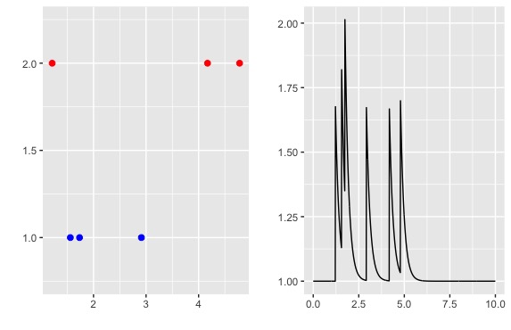
Figure 1: Example of simulation of the 2-dimensional Hawkes process: left the two trains of jump times, right the sum of the intensities $(\lambda^{(j)}_{t})_{t}$ on $[0;10]$.

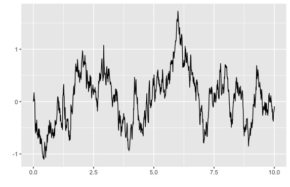
Figure 2: Example of simulation of $X$ for model 1 with $n=100$ and $\Delta=1/10$, with the Hawkes process represented on Figure 4.

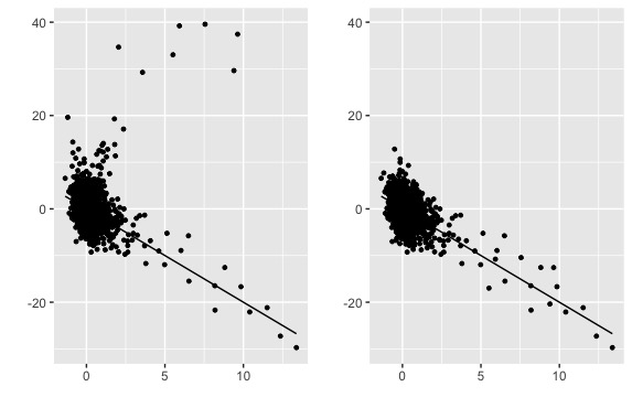
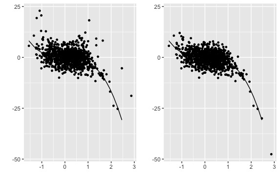
Figure 3: At the left, $Y_{k\Delta}$ versus $X_{k\Delta}$, at the right, $U_{k\Delta}$ versus $X_{k\Delta}$. On the top, model 1, at the bottom, model 2. The true function $b$ is in plain line. Simulations for $n=1000$ and $\Delta=1/10$.

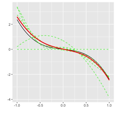
Figure 4: Collection of estimators $\widehat{b}_{m}$ in (green) dotted line, true function $b$ in dark plain line and final estimator $\widehat{b}_{\widehat{m}}$ in red bold line for Model 2.

	$\begin{matrix}n&=1000\\ \Delta&=1/10\end{matrix}$	$\begin{matrix}n&=10000\\ \Delta&=1/10\end{matrix}$	$\begin{matrix}n&=1000\\ \Delta&=1/100\end{matrix}$	$\begin{matrix}n&=10000\\ \Delta&=1/100\end{matrix}$
Model 1	$0.068$	$0.011$	$1.917$	$0.061$
Model 2	$0.080$	$0.007$	$2.948$	$0.104$
Model 3	$0.161$	$0.014$	$4.528$	$0.154$
Model 4	$0.058$	$0.005$	$4.398$	$0.065$

Table 1: Empirical risk $\mathbb{E}[\|\widehat{b}_{\widehat{m}}-b\|_{n}^{2}]$ from 1000 repetitions of Monte-Carlo on $[-1,1]$.

5 Discussion

In this paper, we provide a nonparametric estimator of the drift function in a diffusion process with jumps driven by a Hawkes process. Section 3 is devoted to theoretical guarantees for the non-adaptive and adaptive estimator. Section 4 deals with the implementation of the process and of the estimator.

In future works, we plan to generalize the obtained results. There are many remaining questions of interest. The case of an unknown diffusion coefficient $\sigma$ and an unknown jump coefficient $a$ are obviously crucial issues. Indeed, the presented results require the knowledge of $\sigma_{1}^{2}$ (the square of the bound on volatility, see Assumption 2.1) and of the coefficient $a(\cdot)$ (for the computation of $T_{M}$ in particular). The relation

$$\frac{(X_{(k+1)\Delta}-X_{k\Delta})^{2}}{\Delta}=\sigma^{2}(X_{k\Delta})+a^{2}(X_{k\Delta}){\left(\frac{1}{\Delta}\int_{k\Delta}^{(k+1)\Delta}\sum_{j=1}^{M}{\lambda}^{(j)}_{s}ds\right)}+\text{terms}$$

should lead to some estimation of $\sigma^{2},a,\sigma^{2}+a$ (or at least in the parametric case). Nevertheless it is not a simple issue because the additional terms here are not centered and are hard to control. It will be investigated in future works.

One may also think of generalizing the initial model. For instance, the case of unknown kernel functions $h$ for the Hawkes process is of interest. Indeed, as several nonparametric estimators of $\lambda$ are available (mainly Bacry et al., 2012; Hansen et al., 2015) an estimator of $\lambda$ could be plug-in the procedure of the estimation of the coefficients.

Finally, this estimation procedure will be tested on a neuronal dataset and put in competition with classical methods of machine learning. This is a work in progress.

6 Proofs

We drive the reader attention on the fact that through the proofs the constants are generically noted $C,C^{\prime}...$ for a strictly positive, real-valued constant, not necessarily the same. Sometimes, the notation $C(k)$ is used to emphasize that the constant depends on $k$ in some unspecified manner.

6.1 Preliminary result

Let us remind the reader a result obtained in Bacry et al. (2013), named Lemma 4 and Lemma 6.

Lemma 6.1.

For all $\delta>0$,

1. there exists a positive constant $C$ such that

   $$\sum_{j=1}^{M}\mathbb{E}[(N_{t+\delta}^{(j)}-N_{t}^{(j)})^{2}]\leq C(\delta+\delta^{2}),$$ (6.1)

2. and there exists a positive constant $C$ such that

   $$\sum_{j=1}^{M}\mathbb{E}[(N_{t+\delta}^{(j)}-N_{t}^{(j)})^{4}]\leq C(\delta+\delta^{2}+\delta^{4}).$$ (6.2)

Proof of Lemma 6.1. (i) Following Bacry & Muzy (2014), denoting $A^{(j)}_{t}:=N^{(j)}_{t}-\mathbb{E}[N^{(j)}_{t}]$, it comes

$$\sum_{j=1}^{M}\mathbb{E}[(N_{t+\delta}^{(j)}-N_{t}^{(j)})^{2}] \leq 2\sum_{j=1}^{M}\mathbb{E}[(A_{t+\delta}^{(j)}-A_{t}^{(j)})^{2}]+(\mathbb{E}[(N_{t+\delta}^{(j)}-N_{t}^{(j)}])^{2}$$

$$\leq 2\|\mathbb{E}[N_{t+\delta}-N_{t}]\|^{2}+2\mathbb{E}[\|A_{t+h}-A_{t}\|^{2}]$$

where $\|.\|$ is the Euclidean norm on $\mathbb{R}^{M}$. The first term is controlled by Equation (2.3): $\mathbb{E}[N_{t+\delta}-N_{t}]=\delta(I_{d}-H)^{-1}\xi$ where $\xi$ is the M-vector of $\xi_{j}$’s and $H=(c_{j,k}/\alpha)_{j,k\in\{1,\dots,M\}}$, it is of order $\delta^{2}$. The second term is controlled by Lemma 6 of Bacry et al. (2013) and is of order $\delta$. There are constants that depend on $c_{j,k},\alpha,\xi_{i}$.

(ii) The same notations as in Bacry & Muzy (2014) are used:

$$A_{t}^{(j)}=N_{t}^{(j)}-\mathbb{E}[N_{t}^{(j)}]=\widetilde{N}^{(j)}_{t}+\int_{0}^{t}\sum_{i=1}^{M}\psi_{ij}\widetilde{N}_{s}^{(j)}ds,$$

where $\widetilde{N}_{t}^{(j)}=N_{t}^{(j)}-\int_{0}^{t}\lambda_{t}^{(j)}$ is a local martingale, $\psi_{ij}=\sum_{n\geq 1}h_{n}^{ij}$ and $h_{n}^{ij}$ is such that $h_{n+1}^{ij}(t)=\int_{0}^{t}h_{ij}(t-s)h_{n}^{ij}(s)ds$ and $h_{1}^{ij}=h_{ij}$. With these notations, we have for a constant $C$ that may change from a line to another

$$\mathbb{E}\left[(N_{t+\delta}^{(j)}-N_{t}^{(j)})^{4}\right]\leq C\mathbb{E}\left[(A_{t+\delta}^{(j)}-A_{t}^{(j)})^{4}\right]+C\mathbb{E}\left[N_{t+\delta}^{(j)}-N_{t}^{(j)}\right]^{4}.$$

From Equation (2.3), we have $\mathbb{E}[N_{t+\delta}^{(j)}-N_{t}^{(j)}]^{4}\leq C\delta^{4}$. The second term in the previous inequality can be controlled as follows

$$\mathbb{E}[(A_{t+\delta}^{(j)}-A_{t}^{(j)})^{4}]\leq C\mathbb{E}[(\widetilde{N}_{t+\delta}^{(j)}-\widetilde{N}_{t}^{(j)})^{4}]+C\mathbb{E}\left[\left(\int_{0}^{+\infty}\sum_{i=1}^{M}\psi_{ij}(u)(\widetilde{N}_{t+\delta-u}^{(j)}-\widetilde{N}_{t-u}^{(j)})du\right)^{4}\right].$$

From Bacry & Muzy (2014), Lemma 9, we have

$$\mathbb{E}\left[\underset{t\leq s\leq t+\delta}{\sup}(\widetilde{N}_{s}^{(j)}-\widetilde{N}_{t}^{(j)})^{4}|\mathcal{F}_{t}\right]\leq C(\delta+\delta^{2}).$$

We deduce that

$$\mathbb{E}[(A_{t+\delta}^{(j)}-A_{t}^{(j)})^{4}] \leq C(\delta+\delta^{2})+C\int_{0}^{+\infty}\Big{(}\sum_{i=1}^{M}\psi_{ij}(u)\Big{)}^{4}\mathbb{E}[(\widetilde{N}_{t+\delta-u}^{(j)}-\widetilde{N}_{t-u}^{(j)})^{4}]du$$

$$\leq C(\delta+\delta^{2}).$$

The last inequality holds due the fact that $\int_{0}^{\infty}\Big{(}\sum_{i=1}^{M}\psi_{ij}(u)\Big{)}^{4}du<+\infty$ for every $j=1,\dots,M$. Indeed, for $h_{i,j}=c_{i,j}e^{-\alpha t}$ for $i,j\in\{1,\dots,M\}$, we have

$$h_{n}^{i,j}(t)=c_{i,j}^{n}\dfrac{t^{n-1}}{(n-1)!}e^{-\alpha t}\quad\text{and}\quad\psi_{ij}(t)=\sum_{n\geq 1}h_{n}^{ij}(t)=c_{i,j}e^{-(\alpha-c_{i,j})t}.$$

Thus, if $\alpha\geq c_{i,j}$ for all $i,j\in\{1,\dots,M\}$, we have $\int_{0}^{\infty}\Big{(}\sum_{i=1}^{M}\psi_{ij}(u)\Big{)}^{4}du<+\infty$ for every $j=1,\dots,M$. $\Box$

6.2 Proof of Proposition 2.5

Following Gloter (2000) Proposition 5.1, we first show that for $p=2$ or $p=4$, $\displaystyle\mathbb{E}\left[\underset{s\in[t,t+\delta]}{\sup}|X_{s}|^{p}\Big{|}{\mathcal{F}}_{t}\right]\leq c(p)(1+|X_{t}|^{p})$. Choose $s\in[t,t+\delta]$ with $\delta<1$.

Then,

$$X_{s}-X_{t}=\int_{t}^{s}b(X_{u})du+\int_{t}^{s}\sigma(X_{u})dW_{u}+\sum_{j=1}^{M}\int_{t}^{s}a(X_{u-})dN^{(j)}_{u}.$$

Using Burkholder–Davis–Gundy inequality, the fact that $\sigma$ and $b$ are Lipschitz and that $a$ is bounded, we have for $p=2$ or $p=4$

$$\displaystyle\mathbb{E}\left[\underset{s\in[t,t+\delta]}{\sup}|X_{s}|^{p}\Big{|}{\mathcal{F}}_{t}\right] \leq c(p)|X_{t}|^{p}+c(p)\mathbb{E}\Big{[}\Big{(}\int_{t}^{s}\sigma^{2}(X_{u})du\Big{)}^{p/2}\Big{|}\mathcal{F}_{t}\Big{]}$$

$$+c(p)\mathbb{E}\Big{[}\Big{(}\int_{t}^{s}|b(X_{u})|du\Big{)}^{p}\Big{|}\mathcal{F}_{t}\Big{]}+c(p)\mathbb{E}\Big{[}\Big{(}\sum_{j=1}^{M}\int_{t}^{s}a(X_{u-})dN_{u}^{(j)}\Big{)}^{p}\Big{|}\mathcal{F}_{t}\Big{]}$$

$$\leq c(p)|X_{t}|^{p}+c(p)\mathbb{E}\Big{[}\Big{(}\int_{t}^{s}(|\sigma(X_{u})|^{p}+|b(X_{u})|^{p})du\Big{|}\mathcal{F}_{t}\Big{]}$$

$$+c(p,M)a_{1}^{p}\sum_{j=1}^{M}\mathbb{E}[(N_{s}^{(j)}-N_{t}^{(j)})^{p}|\mathcal{F}_{t}]$$

$$\leq c(p)|X_{t}|^{p}+c(p)\int_{t}^{s}\mathbb{E}[(1+|X_{u}|^{p})|\mathcal{F}_{t}]du+c(p,M)a_{1}^{p}\sum_{j=1}^{M}\mathbb{E}[(N_{s}^{(j)}-N_{t}^{(j)})^{p}|\mathcal{F}_{t}],$$

where the constants may change from a line to another. We then introduce the following notation: $\phi(s)\leq\underset{u\in[t,s]}{\sup}\mathbb{E}[|X_{u}|^{p}|\mathcal{F}_{t}]$. We have with this notation

$$\phi(s)\leq c(p,M)(1+|X_{t}|^{p}+a_{1}^{p}\sum_{j=1}^{M}\mathbb{E}[(N_{s}^{(j)}-N_{t}^{(j)})^{p}|\mathcal{F}_{t}])+c(p)\int_{t}^{s}\phi(u)du.$$

From Assumption 2.1.1, $\phi(s)$ is almost surely finite. We can apply Gronwall’s Lemma (see in Appendix Lemma 7.1) to obtain

$$\phi(s) \leq c(p,M)\Big{(}1+|X_{t}|^{p}+a_{1}^{p}\sum_{j=1}^{M}\mathbb{E}[(N_{s}^{(j)}-N_{t}^{(j)})^{p}|\mathcal{F}_{t}]\Big{)}+c(p)(1+|X_{t}|^{p})(s-t)$$

$$+c(p,M)a_{1}^{p}\int_{t}^{s}\sum_{j=1}^{M}\mathbb{E}[(N_{u}^{(j)}-N_{t}^{(j)})^{p}|\mathcal{F}_{t}]e^{c(p)(t-u)}du.$$

Since $s\in[t,t+\delta]$ and $\delta<1$, applying Lemma 6.1, we obtain

$$\underset{u\in[t,t+\delta]}{\sup}\mathbb{E}[|X_{u}|^{p}|\mathcal{F}_{t}]\leq c(p)(1+|X_{t}|^{p}).$$ (6.3)

Now, we consider $\Delta_{t,t+\delta}:=\underset{s\in[t,t+\delta]}{\sup}|X_{s}-X_{t}|$. As previously, we have

$$\mathbb{E}\left[(\Delta_{t,t+\delta})^{p}|{\mathcal{F}}_{t}\right] \leq c(p)\mathbb{E}\left[\left(\int_{t}^{t+\delta}\sigma^{2}(X_{u})du\right)^{p/2}\Big{|}{\mathcal{F}}_{t}\right]+2\mathbb{E}\left[\left(\int_{t}^{t+\delta}|b(X_{u})|du\right)^{p}\Big{|}{\mathcal{F}}_{t}\right]$$

$$+c(p,M,a_{1})\sum_{j=1}^{M}\mathbb{E}\left[\left(N^{(j)}_{t+\delta}-N^{(j)}_{t}\right)^{p}\Big{|}\bar{\mathcal{F}}_{t}\right]$$

$$\leq c(p)\mathbb{E}\left[\delta^{p/2}\sup_{t\leq s\leq t+\delta}\sigma^{p}(X_{s})+\delta^{p}\sup_{t\leq s\leq t+\delta}|b(X_{s})|^{p}\Big{|}{\mathcal{F}}_{t}\right]$$

$$+c(p,M,a_{1})\sum_{j=1}^{M}\mathbb{E}\left[\left(N^{(j)}_{t+\delta}-N^{(j)}_{t}\right)^{p}\Big{|}\mathcal{F}_{t}\right]$$

and

$$\mathbb{E}\left[(\Delta_{t,t+\delta})^{p}|{\mathcal{F}}_{t}\right] \leq c(p)\delta^{p/2}\leavevmode\nobreak\ \mathbb{E}\left[\sup_{t\leq s\leq t+\delta}(1+|X_{s}|^{p})\Big{|}{\mathcal{F}}_{t}\right]+c(p,M,a_{1})\sum_{j=1}^{M}\mathbb{E}\left[\left(N^{(j)}_{t+\delta}-N^{(j)}_{t}\right)^{p}\Big{|}{\mathcal{F}}_{t}\right].$$

Finally, according to Equations (6.1), (6.2) and (6.3), since $p=2$ or $p=4$, there exists a constant $C(M,a_{1})$, such that

$$\mathbb{E}\left[(\Delta_{t,t+\delta})^{p}\right] \leq C(M,a_{1})\delta(1+\mathbb{E}[|X_{t}|^{p}]).$$

Finally since $\mathbb{E}[X_{t}^{p}]<\infty$, we deduce the assertion. $\Box$

6.3 Additional results

Lemma 6.2.

For $p=2$ or $p=4$, it yields

$$\mathbb{E}\Big{[}\Big{(}\int_{k\Delta}^{(k+1)\Delta}b(X_{k\Delta})-b(X_{s})ds\Big{)}^{p}\Big{]}\leq C(M,a_{1})\Delta^{3p/2}.$$

Proof of Lemma 6.2 According to Cauchy-Schwarz and Jensen’s inequalities, we have

$$\left(\int_{k\Delta}^{(k+1)\Delta}b(X_{k\Delta})-b(X_{s})ds\right)^{p} = \Delta^{p}\left(\frac{1}{\Delta}\int_{k\Delta}^{(k+1)\Delta}b(X_{k\Delta})-b(X_{s})ds\right)^{p}$$

$$\leq \Delta^{p}\left(\frac{1}{\Delta}\int_{k\Delta}^{(k+1)\Delta}(b(X_{k\Delta})-b(X_{s}))^{p}ds\right)$$

$$\leq \Delta^{p-1}\int_{k\Delta}^{(k+1)\Delta}(b(X_{k\Delta})-b(X_{s}))^{p}ds.$$

Applying Proposition 2.5, gives

$$\mathbb{E}\left[\left(\int_{k\Delta}^{(k+1)\Delta}b(X_{k\Delta})-b(X_{s})ds\right)^{p}\right] \leq\Delta^{p-1}\mathbb{E}\left[\int_{k\Delta}^{(k+1)\Delta}(b(X_{k\Delta})-b(X_{s}))^{p}ds\right]$$

$$\leq C(M,a_{1})\Delta^{p+1}.\quad\Box$$

Lemma 6.3.

For some constant $C(M,a_{1})>0$ (depending on $M$ and $a_{1}$) we have

$$\mathbb{E}[I_{k\Delta}^{2}]\leq C(M,a_{1})\Delta,\quad\mathbb{E}[I_{k\Delta}^{4}]\leq C(M,a_{1})\Delta.$$

There exists $C>0$ such that

$$\mathbb{E}[Z_{k\Delta}^{4}|{\mathcal{F}}_{k\Delta}]\leq C\dfrac{\sigma_{1}^{4}}{\Delta^{2}}.$$

Proof of Lemma 6.3
The first point comes from Lemma 6.2 with $p=2$, the second point can be deduced when $p=4$. Finally, with Burkholder–Davis– Gundy inequality we find,

$$\mathbb{E}\left[Z_{k\Delta}^{4}|{\mathcal{F}}_{k\Delta}\right]\leq\frac{C}{\Delta^{4}}\mathbb{E}\left[\left(\int_{k\Delta}^{(k+1)\Delta}\sigma^{2}(X_{s})ds\right)^{2}\Big{|}{\mathcal{F}}_{k\Delta}\right]\leq\frac{C}{\Delta^{4}}\sigma_{1}^{4}\Delta^{2}=C\frac{\sigma_{1}^{4}}{\Delta^{2}}.\quad\Box$$

6.4 Proof of Proposition 3.3

From the definition of the contrast function it comes for $t\in\mathbb{L}^{2}(A)$,

$$\gamma_{n,M}(t)-\gamma_{n,M}(b) = \|t-b\|^{2}_{n}+\frac{2}{n}\sum_{k=1}^{n}(b-t)(X_{k\Delta})I_{k\Delta}+\frac{2}{n}\sum_{k=1}^{n}(b-t)(X_{k\Delta})Z_{k\Delta}.$$

Let us define

$$\mu_{n}(t):=\frac{1}{n}\sum_{k=1}^{n}t(X_{k\Delta})Z_{k\Delta}.$$ (6.4)

By definition of $\widehat{b}_{m}$, we have

$$\gamma_{n,M}(\widehat{b}_{m})-\gamma_{n,M}(b)\leq\gamma_{n,M}({b}_{m})-\gamma_{n,M}(b),$$

where $b_{m}\in\mathcal{S}_{m}$, for example $b_{m}$ is the orthogonal projection of $b$ on $\mathcal{S}_{m}$. This implies

$$\|\widehat{b}_{m}-b\|_{n}^{2} \leq \|{b}_{m}-b\|_{n}^{2}+{\frac{2}{n}\sum_{k=1}^{n}(\widehat{b}_{m}-b_{m})(X_{k\Delta})I_{k\Delta}}+2\mu_{n}(\widehat{b}_{m}-b_{m})$$

(where $b$ denotes the restriction of $b$ to $A$). Let us denote:

$$\mathcal{B}_{m,\pi}=\{t\in\mathcal{S}_{m},\|t\|_{\pi^{X}}=1\},$$

If $t$ is a deterministic function, $\mathbb{E}[\|t\|^{2}_{n}]=\|t\|_{\pi^{X}}^{2}$.

Using Cauchy-Schwarz inequality and the relation $2xy\leq x^{2}/d+dy^{2}$ for $x,y,d>0$, it comes

$$\|\widehat{b}_{m}-b\|_{n}^{2} \leq \|{b}_{m}-b\|_{n}^{2}+2\|\widehat{b}_{m}-b_{m}\|_{n}\left(\frac{1}{n}\sum_{k=1}^{n}I_{k\Delta}^{2}\right)^{1/2}+2\|\widehat{b}_{m}-b_{m}\|_{\pi^{X}}\underset{t\in\mathcal{B}_{m,\pi^{X}}}{\sup}|\mu_{n}(t)|$$

$$\leq \|{b}_{m}-b\|_{n}^{2}+\frac{1}{d}\|\widehat{b}_{m}-b_{m}\|_{\pi^{X}}^{2}+d\underset{t\in\mathcal{B}_{m,\pi^{X}}}{\sup}|\mu_{n}(t)|^{2}+\frac{1}{d}\|\widehat{b}_{m}-b_{m}\|_{n}^{2}+\frac{d}{n}\sum_{k=1}^{n}I_{k\Delta}^{2}.$$

First, let us consider the following set where the $\pi^{X}$-norm and the empiric norm are equivalent:

$$\Omega_{n}:=\left\{\omega,\forall t\in\mathcal{S}\backslash\{0\},\leavevmode\nobreak\ \left|\frac{\|t\|^{2}_{n}}{\|t\|^{2}_{\pi^{X}}}-1\right|\leq 1/2\right\}.$$ (6.5)

Bound of the risk on $\Omega_{n}$
On $\Omega_{n}$, we have $\|\widehat{b}_{m}-b_{m}\|_{\pi^{X}}^{2}\leq 2\|\widehat{b}_{m}-b_{m}\|_{n}^{2}$ and $\|\widehat{b}_{m}-b_{m}\|_{n}^{2}\leq 2(\|\widehat{b}_{m}-b\|_{n}^{2}+\|{b}_{m}-b\|_{n}^{2})$ thus it comes

$$\|\widehat{b}_{m}-b\|_{n}^{2}\leq 13\|{b}_{m}-b\|_{n}^{2}+49\frac{1}{n}\sum_{k=1}^{n}I_{k\Delta}^{2}+49\underset{t\in\mathcal{B}_{m,\pi^{X}}}{\sup}|\mu_{n}(t)|^{2}$$ (6.6)

Denote $(\psi_{\ell})_{\ell}$ an orthogonal basis of $\mathcal{S}_{m}$ for the $\mathbb{L}^{2}_{\pi^{X}}$-norm (thus $\displaystyle\int\psi^{2}_{\ell}(x)\pi^{X}(x)dx=1$). It comes from Cauchy-Schwarz inequality that,

$$\underset{t\in\mathcal{B}_{m,\pi^{X}}}{\sup}|\mu_{n}(t)|^{2}=\underset{\sum_{\ell}\alpha_{\ell}^{2}\leq 1}{\sup}\mu^{2}_{n,M}\left(\sum_{\ell}\alpha_{\ell}\psi_{\ell}\right)\leq\underset{\sum_{\ell}\alpha_{\ell}^{2}\leq 1}{\sup}\left(\sum_{\ell}\alpha_{\ell}^{2}\right)\left(\sum_{\ell}\mu_{n}^{2}(\psi_{\ell})\right)=\sum_{\ell=1}^{D_{m}}\mu_{n}^{2}(\psi_{\ell}).$$ (6.7)

Moreover,

$$\mathbb{E}\left[\underset{t\in\mathcal{B}_{m,\pi^{X}}}{\sup}\mu_{n}^{2}(t)\right] \leq \sum_{\ell=1}^{D_{m}}\mathbb{E}[\mu_{n}^{2}(\psi_{\ell})]$$ (6.8)

$$\leq \frac{2}{n^{2}\Delta^{2}}\sum_{k=1}^{n}\mathbb{E}\left[\sum_{\ell=1}^{D_{m}}\psi_{\ell}^{2}(X_{k\Delta})\mathbb{E}\Big{[}\Big{(}\int_{k\Delta}^{(k+1)\Delta}\sigma(X_{s})dW_{s}\Big{)}^{2}|{\mathcal{F}}_{k\Delta}\Big{]}\right]$$

$$\leq \frac{2}{n^{2}\Delta^{2}}\sum_{k=1}^{n}\mathbb{E}\left[\sum_{\ell=1}^{D_{m}}\psi_{\ell}^{2}(X_{k\Delta})\mathbb{E}\Big{[}\int_{k\Delta}^{(k+1)\Delta}\sigma^{2}(X_{s})ds|{\mathcal{F}}_{k\Delta}\Big{]}\right]$$

$$\leq \frac{2D_{m}\sigma_{1}^{4}}{n\Delta}$$

(if $\sigma$ is not bounded one can use the stationarity of the process). With Lemma 6.3 the obtained result is

$$\mathbb{E}[\|\widehat{b}_{m}-b\|_{n}^{2}\mathds{1}_{\Omega_{n}}]\leq C_{1}\mathbb{E}[\|b-b_{m}\|_{n}^{2}]+C_{2}\frac{D_{m}}{n\Delta}+C_{3}\Delta$$ (6.9)

with $C_{1}=13$, $C_{2}=98\sigma_{1}^{4}$, $C_{3}$ depending on $a_{1},M,\sigma_{1}$.

Bound of the risk on $\Omega_{n}^{c}$

Let us set $e=(e_{\Delta},\dots,e_{n\Delta})$, where $e_{k\Delta}:=U_{k\Delta}-b(X_{k\Delta})=I_{k\Delta}+Z_{k\Delta}$ and $\Pi_{m}U=\Pi_{m}(U_{\Delta},\dots,U_{n\Delta})=(\widehat{b}_{m}(X_{\Delta}),\dots,\widehat{b}_{m}(X_{n\Delta}))$ where $\Pi_{m}$ is the Euclidean orthogonal projection over $\mathcal{S}_{m}$. Then according to the projection definition,

$$\|\widehat{b}_{m}-b\|_{n}^{2} =\|\Pi_{m}U-b\|_{n}^{2}=\|\Pi_{m}b-b\|_{n}^{2}+\|\Pi_{m}U-\Pi_{m}b\|_{n}^{2}$$

$$\leq\|b\|_{n}^{2}+\|U-b\|_{n}^{2}=\|b\|_{n}^{2}+\|e\|_{n}^{2}.$$

Cauchy-Schwarz inequality implies,

$$\mathbb{E}[\|e\|^{4}_{n}] =\mathbb{E}\Big{[}\Big{(}\dfrac{1}{n}\sum_{k=1}^{n}(I_{k\Delta}+Z_{k\Delta})^{2}\Big{)}^{2}\Big{]}$$

$$\leq\dfrac{1}{n}\sum_{k=1}^{n}2^{3}\mathbb{E}\Big{[}I_{k\Delta}^{4}+Z_{k\Delta}^{4}\Big{]}.$$

With the controls given in Lemma 6.3, the additional following result will end the proof.

Lemma 6.4.

If $n\Delta/\ln^{2}(n)\rightarrow\infty$ if $D_{n}\leq O((n\Delta)/(\ln^{2}(n)))$, the probability of the event $\Omega_{n}^{c}$ is bounded as follows:

$$\mathbb{P}(\Omega_{n}^{c})\leq\frac{c_{0}}{n^{4}}.$$

This Lemma is proven in Subsection 6.6.

From Lemma 6.3, Lemma 6.4, Cauchy-Schwarz inequality, we finally obtain

$$\mathbb{E}[\|e\|_{n}^{2}\mathds{1}_{\Omega_{n}^{c}}]\leq\left(\mathbb{E}[\|e\|_{n}^{4}]^{1/2}\right)\left(\mathbb{P}(\Omega_{n}^{c})^{1/2}\right)\leq\dfrac{C}{n\Delta}.$$

Using that $\|\widehat{b}_{m}-b\|_{n}^{2}\leq\|b\|_{n}^{2}+\|e\|_{n}^{2}$, we deduce under the stationarity assumption, that

$$\mathbb{E}[\|\hat{b}_{m}-b\|_{n}^{2}\mathds{1}_{\Omega_{n}^{c}}] \leq \mathbb{E}\left[\frac{1}{n}\sum_{k=1}^{n}b(X_{k\Delta})^{2}\mathds{1}_{\Omega_{n}^{c}}\right]+\mathbb{E}\left[\frac{1}{n}\sum_{k=1}^{n}(e_{k\Delta})^{2}\mathds{1}_{\Omega_{n}^{c}}\right]$$

$$\leq \mathbb{E}\left[b^{2}(X_{0})\mathds{1}_{\Omega_{n}^{c}}\right]+\mathbb{E}\left[e^{2}_{\Delta}\mathds{1}_{\Omega_{n}^{c}}\right]$$

$$\leq \mathbb{E}\left[b^{4}(X_{0})\right]^{1/2}\mathbb{P}(\Omega_{n}^{c})^{1/2}+\mathbb{E}\left[e^{4}_{\Delta}\right]^{1/2}\mathbb{P}(\Omega_{n}^{c})^{1/2}.$$

From the Lipschitz property of $b$, we get $\displaystyle\mathbb{E}[b^{4}(X_{0})]\leq C(1+\mathbb{E}[X_{0}^{4}])<\infty$, and from the Lemma 6.3 $\mathbb{E}[e^{4}_{\Delta}]^{1/2}\leq C^{\prime}/\Delta$, thus

$$E[\|\hat{b}_{m}-b\|_{n}^{2}\mathds{1}_{\Omega_{n}^{c}}]\leq\frac{C^{\prime\prime}}{n\Delta}.$$ (6.10)

Gathering Equation (6.9) and (6.10) gives the attended result. $\Box$

6.5 Proof of Theorem 3.5

On $\Omega_{n}^{c}$, the proof can be lead as in the proof of Proposition 3.3.

On $\Omega_{n}$, by definition of $\hat{m}$, we have $\gamma_{n}(\hat{b}_{\hat{m}})+\text{pen}(\hat{m})\leq\gamma_{n}(\widehat{b}_{m})+\text{pen}(m)$. We deduce with the same computation as previously leading to (6.9) that we have for all $m\in\mathcal{M}_{n}$,

$$\mathbb{E}[\|\widehat{b}_{\widehat{m}}-b\|_{n}^{2}\mathds{1}_{\Omega_{n}}] \leq 13\|{b}_{m}-b\|_{n}^{2}+49C\Delta+49\mathbb{E}\left[\underset{t\in\mathcal{B}_{m,\widehat{m},\pi^{X}}}{\sup}|\mu_{n}(t)|^{2}\mathds{1}_{\Omega_{n}}\right]$$

$$+ 7\text{pen}(m)-7\mathbb{E}[\text{pen}(\widehat{m})],$$

where $\mathcal{B}_{m,m^{\prime},\pi^{X}}=\{h\in S_{m}+S_{m^{\prime}}:\|h\|_{\pi^{X}}\leq 1\}$ and $\mu_{n}$ given in Equation (6.4). The challenge here is to compute the expectation of the supremum on a random ball. Let us introduce the notation

$$G_{m}(m^{\prime}) :=\underset{t\in\mathcal{B}_{m,m^{\prime},\pi^{X}}}{\sup}\leavevmode\nobreak\ |\mu_{n}(t)|.$$

Then,

$$\mathbb{E}[\|\widehat{b}_{\widehat{m}}-b\|_{n}^{2}\mathds{1}_{\Omega_{n}}] \leq 13\mathbb{E}[\|{b}_{m}-b\|_{n}^{2}]+49C\Delta+49\mathbb{E}\left[G_{m}^{2}(\widehat{m})\mathds{1}_{\Omega_{n}}\right]$$

$$+ 7\text{pen}(m)-7\mathbb{E}[\text{pen}(\widehat{m})]$$

$$\leq 13\mathbb{E}[\|{b}_{m}-b\|_{n}^{2}]+49C\Delta+49\sum_{m^{\prime}\in\mathcal{M}_{n}}\mathbb{E}\left[G_{m}^{2}(m^{\prime})-p(m,m^{\prime}))\mathds{1}_{\Omega_{n}}\right]_{+}$$

$$+ 49p(m,\widehat{m})+7\text{pen}(m)-7\mathbb{E}[\text{pen}(\widehat{m})]$$

where $\text{pen}(m)$ must satisfy $7p(m,m^{\prime})\leq\text{pen}(m)+\text{pen}(m^{\prime})$.

To control the term $\displaystyle\mathbb{E}\left[G_{m}^{2}(m^{\prime})-p(m,m^{\prime}))\mathds{1}_{\Omega_{n}}\right]_{+}$ we have to prove a Bernstein-type inequality. Here we follow Baraud et al. (2001b). The idea is presented in Comte et al. (2007) Lemme 2 page 533. We have the following control.

Lemma 6.5.

For any positive numbers $\varepsilon,\leavevmode\nobreak\ v$, we have

$$\mathbb{P}\left(\sum_{k=1}^{n}t(X_{k\Delta})Z_{k\Delta}\geq n\varepsilon,\leavevmode\nobreak\ \|t\|_{n}^{2}\leq v^{2}\right)\leq\exp\left(-\frac{n\varepsilon^{2}\Delta}{2v^{2}\sigma_{1}^{2}}\right).$$

The proof is based on the martingale $\int_{0}^{s}H_{u}dW_{u},\leavevmode\nobreak\ H_{u}=\sum_{k=1}^{n}\mathds{1}_{[k\Delta,(k+1)\Delta[}(u)t(X_{k\Delta})\sigma(X_{u})$ (for the filtration $\sigma(X_{u},\leavevmode\nobreak\ u\leq n\Delta)$), and follows exactly the one detailed in Comte et al. (2007) and is omitted here.

Then, the chaining argument of Baraud et al. (2001b) Proposition 6.1 page 45 can be applied here. We finally obtain:

$$\mathbb{E}\left[G_{m}^{2}(m^{\prime})-p(m,m^{\prime}))\mathds{1}_{\Omega_{n}}\right]_{+}\leq c\sigma_{1}^{2}\frac{e^{-D_{m^{\prime}}}}{n\Delta}$$

and $p(m,m^{\prime})=\rho\sigma^{2}_{0}\frac{D_{m}+D_{m}^{\prime}}{n\Delta}$, thus $\text{pen}(m)\geq 7\rho\sigma_{1}^{2}D_{m}/(n\Delta)$. Finally, we have shown that

$$\mathbb{E}[\|\widehat{b}_{\widehat{m}}-b\|_{n}^{2}\mathds{1}_{\Omega_{n}}] \leq 13\mathbb{E}[\|{b}_{m}-b\|^{2}_{n}]+49C\Delta+49c\sigma_{1}^{2}\sum_{m^{\prime}\in\mathcal{M}_{n}}\frac{e^{-D_{m^{\prime}}}}{n\Delta}+7\text{pen}(m),$$

which ends the proof. $\Box$

6.6 Proof of Lemma 6.4

The proof of this result follows the proof of Lemma 1 of Comte et al. (2007). The difficulty occurs here in the fact that the projection of the invariant measure $\pi$ onto the $X-$ coordinate $\pi^{X}$ is not bounded from below on the compact $A$. Then, the proof must be adapted from Baraud et al. (2001a).

Under the exponential $\beta-$mixing control, similarly to Comte et al. (2007) using Berbee’s coupling method (for the random variables $X_{k\Delta}$), we obtain the decomposition :

$$\mathbb{P}(\Omega_{n}^{c})\leq\mathbb{P}(\Omega_{n}^{c}\cap\Omega^{*})+\mathbb{P}(\Omega^{*c})$$ (6.11)

and

$$\mathbb{P}(\Omega^{*c})\leq n\beta_{X}(q_{n}\Delta)$$

where $q_{n}$ is an integer such that $q_{n}<n$. The notations are those used in Comte et al. (2007), in particular the notation $\text{}^{*}$ referring to the coupling variables is not detailed here.

Let us control the first term now. Let $(\varphi_{j})_{j}=1,\dots,D_{n}$ be an $\mathbb{L}^{2}(A)$-orthonormal basis of $\mathcal{S}_{n}$ and define the matrices:

$$V_{\pi^{X}}=\left[\left(\int_{A}\varphi_{j}^{2}(x)\varphi_{j^{\prime}}^{2}(x)\pi^{X}(x)dx\right)^{1/2}\right]_{j,j^{\prime}\in\{1,\dots,D_{n}\}^{2}},\quad B=\left(\|\varphi_{j}\varphi_{j^{\prime}}\|_{\infty}\right)_{j,j^{\prime}\in\{1,\dots,D_{n}\}^{2}}.$$

Besides, denote $L_{n}(\varphi):=\max(\rho^{2}(V_{\pi^{X}}),\rho(B))$, where for a symmetric matrix $A$:

$$\rho(A):=\sum_{a_{j},\sum_{j}a_{j}^{2}\leq 1}\sum_{j,j^{\prime}}|a_{j}||a_{j}^{\prime}||A_{j,j^{\prime}}|.$$

We note $\mathbb{P}^{*}=\mathbb{P}(\cdot\cap\Omega^{*})$. Let us consider $\nu_{n}(t):=(1/n)\sum_{k=1}^{n}t(X_{k\Delta})-\mathbb{E}[t(X_{k\Delta})]$, $\mathcal{B}_{\pi^{X}}(0,1)=\{t\in\mathcal{S}_{n},\leavevmode\nobreak\ \|t\|_{\pi^{X}}\leq 1\}$ and $\mathcal{B}(0,1)=\{t\in\mathcal{S}_{n},\leavevmode\nobreak\ \|t\|\leq 1\}$, where $\|.\|$ is the $\mathbb{L}^{2}$-norm. As on $A$, $\pi_{0}\leq\pi^{X}(x)$, we have:

$$\sup_{t\in\mathcal{B}_{\pi^{X}}(0,1)}|\nu_{n}(t^{2})|=\sup_{t\in\mathcal{S}_{n}\backslash\{0\}}\left|\frac{\|t\|_{n}^{2}}{\|t\|_{\pi^{X}}^{2}}-1\right|\leq\pi_{0}^{-1}\sup_{t\in\mathcal{B}_{(0,1)}}|\nu(t^{2})|.$$

Thus,

$$\mathbb{P}^{*}\left(\sup_{t\in\mathcal{B}_{\pi^{X}}(0,1)}|\nu_{n}(t^{2})|\geq\rho_{0}\right) \leq \mathbb{P}^{*}\left(\sup_{t\in\mathcal{B}(0,1)}|\nu_{n}(t^{2})|\geq\pi_{0}\rho_{0}\right)$$

$$\leq \mathbb{P}^{*}\left(\sup_{\sum_{j=1}^{D_{n}}a_{j}^{2}\leq 1}\sum_{j,j^{\prime}}|a_{j}a_{j}^{\prime}||\nu(\varphi_{j}\varphi_{j^{\prime}})|\geq\pi_{0}\rho_{0}\right).$$

On the set $\{\forall(j,j^{\prime})\in\{1,\dots,D_{n}\}^{2},\leavevmode\nobreak\ |\nu_{n}(\varphi_{j}\varphi_{j^{\prime}})|\leq 2V_{\pi^{X},j,j^{\prime}}(2x)^{1/2}+3B_{j,j^{\prime}}x\}$ we have

$$\sup_{\sum_{j=1}^{D_{n}}a_{j}^{2}\leq 1}\sum_{j,j^{\prime}}|a_{j}a_{j}^{\prime}||\nu_{n}(\varphi_{j}\varphi_{j^{\prime}})|\leq 2\rho(V_{\pi^{X}})(2x)^{1/2}+3\rho(B)x.$$

Choosing $x=(\rho_{0}\pi_{0})^{2}/(2L_{n}(\varphi))$ with $\rho_{0}=4(1+\sqrt{1+3\pi_{0}})/(3\pi_{0})$ it comes

$$\sup_{\sum_{j=1}^{D_{n}}a_{j}^{2}\leq 1}\sum_{j,j^{\prime}}|a_{j}a_{j}^{\prime}||\nu_{n}(\varphi_{j}\varphi_{j^{\prime}})|\leq\pi_{0}/2.$$

Thus we have obtained:

$$\mathbb{P}^{*}(\Omega_{n}^{c}) = \mathbb{P}^{*}\left(\sup_{t\in\mathcal{B}_{\pi^{X}}(0,1)}|\nu_{n}(t^{2})|\geq 1/2\right)$$

$$\leq \mathbb{P}^{*}\left(\{\forall(j,j^{\prime})\in\{1,\dots,D_{n}\}^{2},\leavevmode\nobreak\ |\nu_{n}(\varphi_{j}\varphi_{j^{\prime}})|\leq 2V_{\pi^{X},j,j^{\prime}}(2x)^{1/2}+3B_{j,j^{\prime}}x\}\right).$$

Then, we have to bound this last probability term. This is done in Baraud et al. (2001a) Claim 6 of Proposition 7 using a Bernstein’s inequality. Let us denote as in Baraud et al. (2001a) $Z^{*}_{l,k}$ the random variables to which the inequality is applied. As the projection of the invariant measure $\pi$ onto the $X-$ coordinate $\pi^{X}$ is not bounded from below, we have only

$$E[(Z^{*}_{l,k})^{2}]\leq\int_{A}\varphi_{j}^{2}(x)\varphi_{j^{\prime}}^{2}(x)\pi^{X}(x)dx=V_{\pi^{X},j,j^{\prime}}$$

and still $\|Z_{l,k}^{*}\|_{\infty}\leq B_{j,j^{\prime}}$. Then, it comes,

$$\mathbb{P}^{*}\left(\{\forall(j,j^{\prime})\in\{1,\dots,D_{n}\}^{2},\leavevmode\nobreak\ |\nu_{n}(\varphi_{j}\varphi_{j^{\prime}})|\leq 2V_{\pi^{X},j,j^{\prime}}(2x)^{1/2}+3B_{j,j^{\prime}}x\}\right)\leq 2D_{n}^{2}\exp\left(-\frac{nx}{q_{n}}\right).$$

The chosen value for $x$ implies that there is a constant $C>0$ such that

$$\mathbb{P}^{*}\left(\{\forall(j,j^{\prime})\in\{1,\dots,D_{n}\}^{2},\leavevmode\nobreak\ |\nu_{n}(\varphi_{j}\varphi_{j^{\prime}})|\leq 2V_{\pi^{X},j,j^{\prime}}(2x)^{1/2}+3B_{j,j^{\prime}}x\}\right)\leq 2D_{n}^{2}\exp\left(-C\frac{n}{q_{n}L_{n}(\varphi)}\right).$$

It remains to control $L_{n}(\varphi)$. Following Lemma 2 of Baraud et al. (2001a) we have for the trigonometric basis according to Cauchy-Schwarz:

$$\rho^{2}(V_{\pi^{X}}) \leq \sum_{j,j^{\prime}\in\{1,\dots,D_{n}\}^{2}}\int_{A}\varphi_{j}^{2}(x)\varphi_{j^{\prime}}^{2}(x)\pi^{X}(x)dx$$

$$\leq \left\|\sum_{j=1}^{D_{n}}\varphi_{j}^{2}\right\|_{\infty}\sum_{j^{\prime}=1}^{D_{n}}\int_{A}\varphi_{j^{\prime}}^{2}(x)\pi^{X}(x)dx$$

$$\leq \phi_{\pi^{X}}\phi_{1}^{2}D_{n}^{2}$$

under Assumption 3.2.1 and 3.2.3. $\rho(B)\leq\phi_{1}^{2}D_{n}$. Thus, $L_{n}(\varphi)\leq\max(1,\phi_{\pi^{X}})\phi_{1}^{2}D_{n}^{2}$. Now, following Equation (2.4), $\beta_{X}(q_{n}\Delta)\leq e^{-\theta q_{n}\Delta}$, decomposition (6.11) leads to

$$\mathbb{P}(\Omega_{n}^{c})\leq 1/n^{4}+2n^{2}\exp\left(-C^{\prime}\frac{n\Delta}{\ln(n)D_{n}}\right),$$

with $q_{n}=\lfloor 5\ln(n)/(\theta\Delta)\rfloor+1$. Finally, for the trigonometric basis, if $\displaystyle D_{n}^{2}\leq\frac{C^{\prime}n\Delta}{6\ln^{2}(n)}$ thus $D_{n}\leq C^{\prime}\sqrt{n\Delta}/\ln(n)$ and $\mathbb{P}(\Omega_{n}^{c})\leq c/n^{4}$, if $n\Delta/\ln^{2}(n)\rightarrow\infty$. $\Box$

7 Appendix: theoretical results

7.1 Gronwall’s Lemma

Lemma 7.1.

Let $\phi$, $\psi$ and $y$ be three non negative continuous functions on $[a,b]$, that satisfy

$$\forall t\in[a,b],\quad y(t)\leq\phi(t)+\int_{a}^{t}\psi(s)y(s)ds.$$

Then

$$\forall t\in[a,b],\quad y(t)\leq\phi(t)+\int_{a}^{t}\phi(s)\psi(s)\exp\Big{(}\int_{s}^{t}\psi(u)du\Big{)}ds.$$

7.2 Talagrand’s inequality

The following result follows from the Talagrand concentration inequality (see Klein & Rio, 2005).

Theorem 7.2.

Consider $n\in\mathbb{N}^{*}$, $\mathcal{F}$ a class at most countable of measurable functions, and $(X_{i})_{i\in\{1,...,n\}}$ a family of real independent random variables. One defines, for all $f\in\mathcal{F}$,

$$\nu_{n}(f)=\frac{1}{n}\sum_{i=1}^{n}(f(X_{i})-\mathbb{E}[f(X_{i})]).$$

Supposing there are three positive constants $M$, $H$ and $v$ such that $\underset{f\in\mathcal{F}}{\sup}\|f\|_{\infty}\leq M$,
$\mathbb{E}[\underset{f\in\mathcal{F}}{\sup}|\nu_{n}(f)|]\leq H$, and $\underset{f\in\mathcal{F}}{\sup}({1}/{n})\sum_{i=1}^{n}\mathrm{Var}(f(X_{i}))\leq v$, then for all $\alpha>0$,

$$\mathbb{E}\left[\left(\underset{f\in\mathcal{F}}{\sup}|\nu_{n}(f)|^{2}-2(1+2\alpha)H^{2}\right)_{+}\right] \leq \frac{4}{b}\left(\frac{v}{n}\exp\left(-b\alpha\frac{nH^{2}}{v}\right)\right.$$

$$+ \left.\frac{49M^{2}}{bC^{2}(\alpha)n^{2}}\exp\left(-\frac{\sqrt{2}bC(\alpha)\sqrt{\alpha}}{7}\frac{nH}{M}\right)\right)$$

with $C(\alpha)=(\sqrt{1+\alpha}-1)\wedge 1$, and $b=\frac{1}{6}$.

References

- Amorino & Gloter (2018) Amorino, C. & Gloter, A. (2018). Contrast function estimation for the drift parameter of ergodic jump diffusion process. arXiv preprint arXiv:1807.08965 .
- Bacry et al. (2012) Bacry, E., Dayri, K. & Muzy, J. (2012). Non-parametric kernel estimation for symmetric hawkes processes. application to high frequency financial data. THE EUROPEAN .
- Bacry et al. (2013) Bacry, E., Delattre, S., Hoffmann, M. & Muzy, J.-F. (2013). Some limit theorems for hawkes processes and application to financial statistics. Stochastic Processes and their Applications 123, 2475–2499.
- Bacry et al. (2015) Bacry, E., Mastromatteo, I. & Muzy, J.-F. (2015). Hawkes processes in finance. Market Microstructure and Liquidity 1, 1550005.
- Bacry & Muzy (2014) Bacry, E. & Muzy, J.-F. (2014). Second order statistics characterization of hawkes processes and non-parametric estimation. arXiv preprint arXiv:1401.0903 .
- Baraud (2002) Baraud, Y. (2002). Model selection for regression on a random design. ESAIM: Probability and Statistics 6, 127–146.
- Baraud et al. (2001a) Baraud, Y., Comte, F. & Viennet, G. (2001a). Adaptive estimation in autoregression or -mixing regression via model selection. Ann. Statist. 29, 839–875. doi:10.1214/aos/1009210692.
- Baraud et al. (2001b) Baraud, Y., Comte, F. & Viennet, G. (2001b). Model selection for (auto-)regression with dependent data. ESAIM: Probability and Statistics 5, 33–49.
- Bibby & Sørensen (1995) Bibby, B. M. & Sørensen, M. (1995). Martingale estimation functions for discretely observed diffusion processes. Bernoulli pp. 17–39.
- Bonnet et al. (2018) Bonnet, A., Rivoirard, V. & Picard, F. (2018). Modeling spatial genomic interactions with the hawkes model. bioRxiv p. 214874.
- Brémaud & Massoulié (1996) Brémaud, P. & Massoulié, L. (1996). Stability of nonlinear hawkes processes. The Annals of Probability pp. 1563–1588.
- Carmona et al. (2013) Carmona, R., Fouque, J.-P. & Sun, L.-H. (2013). Mean field games and systemic risk. Available SSRN .
- Comte & Genon-Catalot (2019) Comte, F. & Genon-Catalot, V. (2019). Nonparametric drift estimation for iid paths of stochastic differential equations. hal-02083474 .
- Comte et al. (2007) Comte, F., Genon-Catalot, V. & Rozenholc, Y. (2007). Penalized nonparametric mean square estimation of the coefficients of diffusion processes. Bernoulli 13, 514–543.
- Daley & Vere-Jones (2007) Daley, D. & Vere-Jones, D. (2007). An introduction to the theory of point processes: volume II: general theory and structure. Springer Science & Business Media.
- Dassios & Zhao (2013) Dassios, A. & Zhao, H. (2013). Exact simulation of hawkes process with exponentially decaying intensity. Electronic Communications in Probability 18, 1–13.
- Delattre et al. (2016) Delattre, S., Fournier, N. & Hoffmann, M. (2016). Hawkes processes on large networks. The Annals of Applied Probability 26, 216–261.
- DeVore & Lorentz (1993) DeVore, R. & Lorentz, G. (1993). Constructive approximation, vol. 303. Springer Science & Business Media.
- Dion (2014) Dion, C. (2014). New adaptive strategies for nonparametric estimation in linear mixed models. Journal of Statistical Planning and Inference 150, 30 – 48.
- Dion et al. (2019) Dion, C., Lemler, S. & Löcherbach, E. (2019). Exponential ergodicity for diffusions with jumps driven by a hawkes process. arXiv preprint arXiv:1904.06051 .
- Ditlevsen & Löcherbach (2017) Ditlevsen, S. & Löcherbach, E. (2017). Multi-class oscillating systems of interacting neurons. Stochastic Processes and their Applications 127, 1840–1869.
- Donnet & Samson (2013) Donnet, S. & Samson, A. (2013). A review on estimation of stochastic differential equations for pharmacokinetic/pharmacodynamic models. Advanced Drug Delivery Reviews 65, 929–939.
- Duarte et al. (2016) Duarte, A., Galves, A., Löcherbach, E. & Ost, G. (2016). Estimating the interaction graph of stochastic neural dynamics. arXiv preprint arXiv:1604.00419 .
- El Karoui et al. (1997) El Karoui, N., Peng, S. & Quenez, M.-C. (1997). Backward stochastic differential equations in finance. Mathematical finance 7, 1–71.
- Gloter (2000) Gloter, A. (2000). Discrete sampling of an integrated diffusion process and parameter estimation of the diffusion coefficient. ESAIM: Probability and Statistics 4, 205–227.
- Gobet (2002) Gobet, E. (2002). Lan property for ergodic diffusions with discrete observations. Ann. Inst. H. Poincaré Probab. Statist. 38, 711–737.
- Gobet et al. (2004) Gobet, E., Hoffmann, M. & Reiß, M. (2004). Nonparametric estimation of scalar diffusions based on low frequency data. The Annals of Statistics 32, 2223–2253.
- Gobet & Matulewicz (2016) Gobet, E. & Matulewicz, G. (2016). Parameter estimation of ornstein–uhlenbeck process generating a stochastic graph. Statistical Inference for Stochastic Processes pp. 1–25.
- Györfi et al. (2006) Györfi, L., Kohler, M., Krzyzak, A. & Walk, H. (2006). A distribution-free theory of nonparametric regression. Springer Science & Business Media.
- Hansen et al. (2015) Hansen, N., Reynaud-Bouret, P. & Rivoirard, V. (2015). Lasso and probabilistic inequalities for multivariate point processes. Bernoulli 21, 83–143. doi:10.3150/13-BEJ562.
- Has’minskii (1980) Has’minskii, R. (1980). Stochastic stability of differential equations. Sijthoff & Noordhoff.
- Hawkes (1971) Hawkes, A. (1971). Spectra of some self-exciting and mutually exciting point processes. Biometrika 58, 83–90. ISSN 00063444. URL http://www.jstor.org/stable/2334319.
- Hawkes & Oakes (1974) Hawkes, A. & Oakes, D. (1974). A cluster process representation of a self-exciting process. Journal of Applied Probability 11, 493–503.
- Hoffmann (1999) Hoffmann, M. (1999). Adaptive estimation in diffusion processes. Stochastic processes and their Applications 79, 135–163.
- Höpfner (2007) Höpfner, R. (2007). On a set of data for the membrane potential in a neuron. Mathematical Biosciences 207, 275 – 301.
- Höpfner et al. (2016) Höpfner, R., Löcherbach, E. & Thieullen, M. (2016). Ergodicity and limit theorems for degenerate diffusions with time periodic drift. application to a stochastic hodgkin- huxley model. ESAIM: Probability and Statistics 20, 527–554.
- Jahn et al. (2011) Jahn, P., Berg, R., Hounsgaard, J. & Ditlevsen, S. (2011). Motoneuron membrane potentials follow a time inhomogeneous jump diffusion process. J. Comput. Neurosci. 31, 563–579.
- Jaisson & Rosenbaum (2015) Jaisson, T. & Rosenbaum, M. (2015). Limit theorems for nearly unstable hawkes processes. The Annals of Applied Probability 25, 600–631.
- Kessler & Sørensen (1999) Kessler, M. & Sørensen, M. (1999). Estimating equations based on eigenfunctions for a discretely observed diffusion process. Bernoulli 5, 299–314.
- Kirchner (2017) Kirchner, M. (2017). An estimation procedure for the hawkes process. Quantitative Finance 17, 571–595.
- Klein & Rio (2005) Klein, T. & Rio, E. (2005). Concentration around the mean for maxima of empirical processes. The Annals of Probability 33, 1060–1077.
- Le Gall (2010) Le Gall, J. (2010). Calcul stochastique et processus de markov. Notes de cours .
- Lemonnier & Vayatis (2014) Lemonnier, R. & Vayatis, N. (2014). Nonparametric markovian learning of triggering kernels for mutually exciting and mutually inhibiting multivariate hawkes processes. In Joint European Conference on Machine Learning and Knowledge Discovery in Databases, pp. 161–176. Springer.
- Lukasik et al. (2016) Lukasik, M., Srijith, P., Vu, D., Bontcheva, K., Zubiaga, A. & Cohn, T. (2016). Hawkes processes for continuous time sequence classification: an application to rumour stance classification in twitter. Proceedings of the 54th Annual Meeting of the Association for Computational Linguistics (Volume 2: Short Papers) 2, 393–398.
- Mancini (2009) Mancini, C. (2009). Non-parametric threshold estimation for models with stochastic diffusion coefficient and jumps. Scandinavian Journal of Statistics 36, 270–296.
- Masuda (2007) Masuda, H. (2007). Ergodicity and exponential -mixing bounds for multidimensional diffusions with jumps. Stochastic processes and their applications 117, 35–56.
- Parisi & Sourlas (1992) Parisi, G. & Sourlas, N. (1992). Supersymmetric field theories and stochastic differential equations. World Scientific.
- Rambaldi et al. (2015) Rambaldi, M., Pennesi, P. & Lillo, F. (2015). Modeling foreign exchange market activity around macroeconomic news: Hawkes-process approach. Phys. Rev. E 91, 012819.
- Renault & Touzi (1996) Renault, E. & Touzi, N. (1996). Option hedging and implied volatilities in a stochastic volatility model 1. Mathematical Finance 6, 279–302.
- Reynaud-Bouret et al. (2013) Reynaud-Bouret, P., Rivoirard, V. & Tuleau-Malot, C. (2013). Inference of functional connectivity in neurosciences via hawkes processes. In Global Conference on Signal and Information Processing (GlobalSIP), 2013 IEEE, pp. 317–320. IEEE.
- Reynaud-Bouret & Roy (2007) Reynaud-Bouret, P. & Roy, E. (2007). Some non asymptotic tail estimates for hawkes processes. Bulletin of the Belgian Mathematical Society-Simon Stevin 13, 883–896.
- Schmisser (2014a) Schmisser, E. (2014a). Nonparametric adaptive estimation of the drift for a jump diffusion process. Stochastic Processes and ther Applications pp. 883–914.
- Schmisser (2014b) Schmisser, E. (2014b). Nonparametric estimation of coefficients of a diffusion with jumps. Hal .
- Shimizu & Yoshida (2006) Shimizu, Y. & Yoshida, N. (2006). Estimation of parameters for diffusion processes with jumps from discrete observations. Statistical Inference for Stochastic Processes 9, 227–277.
- Tankov & Voltchkova (2009) Tankov, P. & Voltchkova, E. (2009). Jump-diffusion models: a practitioner’s guide. Banque et Marchés 99, 24.
- Vasicek (1977) Vasicek, O. (1977). An equilibrium characterization of the term structure. Journal of financial economics 5, 177–188.
- Vere-Jones & Ozaki (1982) Vere-Jones, D. & Ozaki, T. (1982). Some examples of statistical estimation applied to earthquake data. Annals of the Institute of Statistical Mathematics 34, 189–207.
- Veretennikov (1997) Veretennikov, A. (1997). On polynomial mixing bounds for stochastic differential equations. Stochastic Processes and their Applications 70, 115 – 127. ISSN 0304-4149.