Bayesian Approach for Linear Optics Correction

Abstract

With a Bayesian approach, the linear optics correction algorithm for storage rings is revisited. Starting from the Bayes’ theorem, a complete linear optics model is simplified as “likelihood functions” and “prior probability distributions”. Under some assumptions, the least square algorithm and then the Jacobian matrix approach can be re-derived. The coherence of the correction algorithm is ensured through specifying a self-consistent regularization coefficient to prevent overfitting. Optimal weights for different correction objectives are obtained based on their measurement noise level. A new technique has been developed to resolve degenerated quadrupole errors when observed at a few select BPMs. A necessary condition of being distinguishable is that their optics response vectors seen at these specific BPMs should be near-orthogonal.

I introduction

At modern particle accelerator facilities, advanced beam diagnostics instruments with high acquisition rate can generate copious amounts of data within a short time period. The data can be used in a wide variety of applications such as characterizing machine parameters, monitoring machine performance, realizing real-time correction, feedbacks, etc. A specific example would be obtaining beam turn-by-turn (TbT) data from beam position monitors (BPM) after the beam is disturbed. The linear optics functions, such as, the envelope function $\beta$ of betatron oscillation and its phase $\phi$ Courant and Snyder (1958), can be extracted Castro-Garcia (1996); Irwin et al. (1999); Huang et al. (2005). Due to various measurement noise, accurately identifying quadrupole error sources is important for optics correction. One can average over repetitive measurements, then use the mean values directly. Distributions of measurement noise, which are usually ignored, however, can provide rich information for identifying error sources precisely. Using a Bayesian approach and the information provided by the error analysis, the linear optics correction problem presented by accelerators can be approached from the viewpoint of probability.

Lattice measurement noise and quadrupole excitations errors are usually randomly distributed around their expectation values. Overfitting quadrupole errors must be avoided. Specifically, the optics functions $\beta$ and $\phi$ can be measured with BPMs at many locations $s_{i}$, where $i=0,1,\cdots,N-1$, and $N$ is the total number of BPMs. Given a set of measured data with noise, fitting the actual quadrupole errors $\Delta K$, is a typical nonlinear regression problem since the dependence of $\beta$ and $\phi$ on $K$ is nonlinear. In regression problems, overfitting is a modeling error which occurs when a function is too closely fit to a limited set of data points Bishop (2006); Abu-Mostafa et al. (2012). There are two reasons of revisiting this problem with a Bayesian approach. First, the Bayesian approach is a proven technique in preventing overfitting. Second, several optics distortions caused by quadrupole errors need to be corrected simultaneously, but measured in different units and scales. With the Bayesian approach, the coherence of the correction algorithm, which is capable of dealing with multi-objective regression problems, can be established.

In some scenarios, an optics distortion pattern is indeed caused by a single quadrupole error rather than normally distributed errors. However, the goal of the Bayesian approach is to distribute the error to multiple sources. It can sometimes fail to distinguish the single source from its highly degenerated neighbors. A new technique has been developed where only a few specific BPMs are selected to address the degeneracy. One necessary condition for being distinguishable is that the optics response vectors of those specific BPMs should be near-orthogonal.

To further explain this approach, the remaining sections are outlined as follows: Sect. II briefly review the well-known correction scheme, i.e., use of Jacobian matrix as well as a discussion of the difficulties of this method. In Sect. III, we start from the Bayesian theorem to re-derive the least square algorithm. It will become clear that using Jacobian matrix is a simplified version of Bayesian approach with a flat prior probability. Sect. IV introduces a new technique for resolving the degeneracy of neighboring quadrupoles. Both simulation and experimental data taken from the National Synchrotron Light Source II (NSLS-II) storage ring are used to illustrate this technique. A brief summary is given in Sect. V.

II Jacobian matrix approach

A linear optics model of a storage ring can be represented by a set of $s$-dependent optics functions. For simplicity’s sake, the envelope function $\beta(s)$ is used as an example. Other lattice functions such as betatron phase, $\phi(s)$ will be covered later. Given a fixed magnetic lattice layout, an optics model reads as

$$\beta=\beta(s,\boldsymbol{K}),$$ (1)

here $\boldsymbol{K}$ is a vector composed of all normalized quadrupole focusing strengths, and $s$ is the longitudinal coordinate. Bold symbols, such as “$\boldsymbol{X}$”, are used to denote vectors and matrices throughout this paper. The design lattice model is represented as

$$\beta_{0}(s)=\beta(s,\boldsymbol{K}_{0}),$$ (2)

where $\boldsymbol{K}_{0}$ represents the quadrupoles’ nominal setting, $\beta_{0}$ is the nominal envelope function along $s$. If quadrupoles have some errors $\Delta\boldsymbol{K}$ on top of $\boldsymbol{K}_{0}$, the linear lattice is distorted as

$$\beta=\beta_{0}+\Delta\beta=\beta(s,\boldsymbol{K}_{0}+\Delta\boldsymbol{K}).$$ (3)

$\Delta\beta$ is often referred to as $\beta$-beat.

Given the total distribution of $N$ BPMs, a ring’s optics model can be simply represented as an $N$-dimensional vector. Once the linear optics is measured at these BPMs, the lattice correction needs to identify (account for) the actual quadrupole errors. A well-known and straightforward correction method is to use the linear dependence of the $\beta$-function on each quadrupole, i.e., its Jacobian matrix Huang et al. (2005),

$$M_{i,j}=\frac{\partial\beta_{s_{i}}}{\partial K_{j}},$$ (4)

where $s_{i}$ is the $i^{th}$ BPM’s longitudinal location, and $j$ is the index of quadrupoles. $\boldsymbol{M}$ can be constructed based on either a design model or a beam-based measurement. By solving the following equation

$$\Delta\boldsymbol{\beta}=\boldsymbol{M}\cdot\Delta\boldsymbol{K},$$ (5)

the error sources $\Delta\boldsymbol{K}$ can be identified approximately. Here $\Delta\boldsymbol{\beta}$ is a vector of the $\beta$-beat seen at the BPMs. Since the dependence isn’t linear, iteratively applying Eq. (5) is needed.

It turns out that, due to measurement noise, highly degenerated quadrupoles and even bad BPMs, the solution to Eq. (5) is spoiled by overfitting. It is well-known that overfitting can be prevented by a regularization technique Bishop (2006); Abu-Mostafa et al. (2012); Huang et al. (2007). But how to choose a reasonable regularization coefficient to cut off measurement noise isn’t obvious here. At the same time, multiple optics functions are measured, but in different scales and units. We can stack their response matrices vertically with some weights. However, the strategy for specifying appropriate weights isn’t clear. An inappropriate regularization and weight specification could degrade the performance of correction. For example, some functions are overfitted and can sacrifice others. Another concern is that the quadrupole errors obtained with Eq. (5) usually reproduce the optics distortions at the location of the BPMs rather than the whole ring. This might be a critical issue for collider rings, in which no BPM can sit exactly at their interaction points (IP). Minimizing the $\beta$-beat at IP’s neighboring BPMs doesn’t ensure that the optics at IPs are optimized. Therefore, it is important to precisely identify errors in order to correct lattice distortion globally, rather than limited to the locations of BPMs. Some of these difficulties can be mitigated by using a complete accelerator model instead of its Jacobian matrix. Another method is to validate the obtained quadrupole errors at a few testing BPMs, which are intentionally left out from the fitting. However, iterative fitting and validation with a complete optics model is time-consuming, especially for large scale storage rings. In the next section, the lattice correction problem will be addressed using the Bayesian approach.

III Bayesian approach

From the viewpoint of probability, identifying quadrupole errors from repetitive and independent measurements can be achieved by computing a posterior conditional probability distribution and determining its maxima. Consider a simple case of $\beta$ function in the horizontal plane. Based on the Bayes’ theorem, the conditional probability of having an error $\Delta\boldsymbol{K}$ with a measured $\boldsymbol{\beta}$ reads as Bishop (2006); Bernardo

$$p(\Delta\boldsymbol{K}|\boldsymbol{\beta}) = \frac{p(\boldsymbol{\beta}|\Delta\boldsymbol{K})p(\Delta\boldsymbol{K})}{p(\boldsymbol{\beta})}$$ (6)

$$\propto p(\boldsymbol{\beta}|\Delta\boldsymbol{K})p(\Delta\boldsymbol{K}).$$

Eq. (6) can be interpreted as, given a measured optics distortion $\boldsymbol{\beta}=\boldsymbol{\beta_{0}}+\Delta\boldsymbol{\beta}$, the probability of it being the error source of $\Delta\boldsymbol{K}$ is proportional to the product of a likelihood function $p(\boldsymbol{\beta}|\Delta\boldsymbol{K})$ and a probability distribution of error $\Delta\boldsymbol{K}$. The likelihood function can be recognized as being related to the dependence of $\beta$ on $K$, i.e., the Jacobian matrix of Eq. (4). $p(\Delta\boldsymbol{K})$ is known as prior probability distribution which will be covered in greater detail later. $p(\boldsymbol{\beta})$ is the normalizing constant.

By maximizing the probability in Eq. (6), the most likely quadrupole error distribution can be obtained. In general, we can assume that both $\beta$ measurement noise and quadrupole excitation errors are normally distributed. For example, at a particular BPM, repetitive measurement of $\beta$s are distributed around an expectation value $\mathbb{E}(\beta)=\bar{\beta}$ with a variance $\sigma_{\beta}$.

$$\mathcal{N}(\beta|\bar{\beta},\sigma_{\beta}^{2})=\frac{1}{\sqrt{2\pi}\sigma_{\beta}}\exp\left[-\frac{(\beta-\bar{\beta})^{2}}{2\sigma_{\beta}^{2}}\right].$$ (7)

Eq. (6) thus can be re-written as

$$p(\Delta\boldsymbol{K}|\boldsymbol{\beta})\propto\mathcal{N}(\boldsymbol{\beta}|\boldsymbol{\bar{\beta}}(s_{i},\Delta\boldsymbol{K}),\sigma^{2}_{\beta})\cdot\mathcal{N}(\Delta{\boldsymbol{K}}|\boldsymbol{K}_{0},\sigma^{2}_{K}).$$ (8)

Where $\sigma_{K}$ is the variance of quadrupole error distribution. Maximizing the probability of Eq. (8) is equivalent to minimizing its negative logarithm,

$$-\ln\left[p(\Delta\boldsymbol{K}|\boldsymbol{\beta})\right] \propto \frac{1}{2\sigma^{2}_{\beta}}\sum_{i}\left[\beta(s_{i},\Delta\boldsymbol{K})-\bar{\beta}(s_{i})\right]^{2}+$$ (9)

$$\frac{1}{2\sigma^{2}_{K}}\|\Delta\boldsymbol{K}\|^{2}.$$

Here $\|\bullet\|$ is the Euclidean norm of a vector. Eq. (9) can be recognized as the least-square algorithm but with some well-defined weights. It is important to note that, since we assume a normal distribution for quadrupole errors, the solution to Eq. (9) is intended to allocate errors according to a normal distribution, even if they are not. If there is a systematic calibration error on the quadrupole excitations, the second distribution in Eq. (8) has an non-zero mean. But after the first several iterations, the non-zero mean value should be able to be filtered out. A more detailed discussion on a single outlier of quadrupole error will be addressed in Sect. IV.

Now we take a look at the first term on the right-hand side of Eq. (9). By expanding $\beta$ with respect to quadrupole errors $\Delta{\boldsymbol{K}}$ at $\beta_{0}$ and keeping the linear components, it reads as

$$\frac{1}{2\sigma^{2}_{\beta}}\sum_{i}\left[\beta_{0}(s_{i})+\frac{\partial\beta(s_{i})}{\partial\boldsymbol{K}}\Delta{\boldsymbol{K}}-\bar{\beta}(s_{i})\right]^{2}$$ (10)

$$= \frac{1}{2\sigma^{2}_{\beta}}\sum_{i}\left[\frac{\partial\beta(s_{i})}{\partial\boldsymbol{K}}\Delta{\boldsymbol{K}}-\Delta\bar{\beta}(s_{i})\right]^{2},$$

where $\Delta\bar{\beta}(s_{i})=\bar{\beta}_{0}(s_{i})-\beta_{0}(s_{i})$. After differentiating every term with respect to $\Delta\boldsymbol{K}$ and expressing it in the format of a matrix, we obtain the well-known Eq. (5). The solution to Eq. (5) is given as

$$\Delta\boldsymbol{K}=\left[\boldsymbol{M}^{T}\boldsymbol{M}\right]^{-1}\boldsymbol{M}^{T}\Delta\boldsymbol{\bar{\beta}}.$$ (11)

$\left[\boldsymbol{M}^{T}\boldsymbol{M}\right]^{-1}\boldsymbol{M}^{T}$ is often known as the pseudo inverse of $\boldsymbol{M}$, because $\boldsymbol{M}$ is usually non-invertible.

Thus far, the measurement noise $\sigma_{\beta}$ has been ignored. The solution to Eq. (11) often overfits quadrupole errors from either noisy BPM data, or even bad BPMs if they are present. The overfitting can be mitigated by taking the second term into account, which is known as regularization technique. By adding an additional penalty term to the sum of squares in Eq. (9), one can prevent the fitted quadrupole errors from deviating from a reasonable normal distribution. In other words, a complete linear optics model provides not only a likelihood function but an informative prior probability distribution of quadrupole errors as well. The solution to the least-squares problem with regularization is

$$\Delta\boldsymbol{K}=\left[\boldsymbol{M}^{T}\boldsymbol{M}+\lambda\boldsymbol{I}\right]^{-1}\boldsymbol{M}^{T}\Delta\boldsymbol{\bar{\beta}}$$ (12)

It is important to note that the optimal regularization coefficient $\lambda=\frac{\sigma^{2}_{\beta}}{\sigma^{2}_{K}}$ is well-defined here. More specifically, the variance $\sigma_{k}(\Delta\bar{\beta})$ of the quadrupole error distribution $p(\Delta\boldsymbol{K})$ should be determined by the measured $\beta$-beat level using the designed lattice model. Fig. 1 illustrates that the horizontal $\beta$-beat is linearly proportional to the variance of quadrupole error distribution at the NSLS-II ring. After averaging repetitive $\beta_{x}$ measurements and comparing against the nominal $\beta_{x,0}$, the variance of quadrupole error probability distribution $\sigma_{k}(\Delta\bar{\beta})$ can be determined with Fig. 1. During an iterative correction, $\beta$-beat reduces gradually, as do the corresponding quadrupole errors. Therefore the regularization coefficient should be dynamically adjusted to speed up the convergence as well. The $p(\Delta\boldsymbol{K})$ is named as the prior probability because it can be estimated analytically Courant and Snyder (1958) or numerically in advance. In the previous section, one can still use the regularization technique to avoid overfitting, but the coefficient is not necessarily optimal due to lack of a theoretical basis. Experimentally one can obtain this regularization coefficient based on correction performance on a trial basis Huang et al. (2007). However, the Bayesian approach can explicitly give its statistic and physics interpretation.

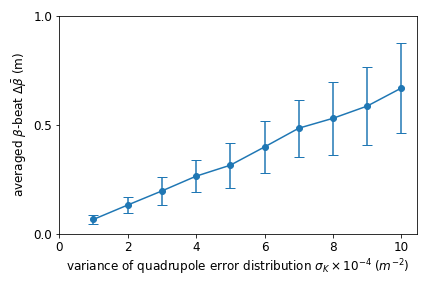
Figure 1: Statistic illustration of the horizontal $\beta$-beat due to the random quadrupole errors. This linear correlation with gradually increasing variance are calculated with the NSLS-II ring lattice model in advance. Once an averaged $\beta$-beat is measured, its corresponding variance of quadrupole error distribution can be used as the prior probability to prevent overfitting

Now consider the case of having multiple correction objectives. With precisely aligned TbT data, the betatron oscillation envelope function $\beta$ and its phase $\phi$ can be obtained simultaneously. The strategy for balancing the correction among multiple objectives is straightforward in the Bayesian approach. The probability of having an error $\Delta\boldsymbol{K}$ with given measured $\boldsymbol{\beta}$ and $\boldsymbol{\phi}$ is a product of two conditional probability distributions

$$p(\Delta\boldsymbol{K}|\boldsymbol{\beta},\boldsymbol{\phi}) \approx \frac{p(\boldsymbol{\beta}|\Delta\boldsymbol{K})p(\boldsymbol{\phi}|\Delta\boldsymbol{K})p(\Delta\boldsymbol{K})}{p(\boldsymbol{\beta},\boldsymbol{\phi})}$$ (13)

$$\propto p(\boldsymbol{\beta}|\Delta\boldsymbol{K})p(\boldsymbol{\phi}|\Delta\boldsymbol{K})p(\Delta\boldsymbol{K}).$$

Maximizing the probability yields

$$-\ln\left[p(\Delta\boldsymbol{K}|\boldsymbol{\beta},\boldsymbol{\phi})\right] \propto \frac{1}{2\sigma^{2}_{\beta}}\sum_{i}\left[\boldsymbol{\beta}(s_{i},\Delta\boldsymbol{K})-\boldsymbol{\bar{\beta}}(s_{i})\right]^{2}+$$ (14)

$$\frac{1}{2\sigma^{2}_{\phi}}\sum_{i}\left[\boldsymbol{\phi}(s_{i},\Delta\boldsymbol{K})-\boldsymbol{\bar{\phi}}(s_{i})\right]^{2}+$$

$$\frac{1}{2\sigma^{2}_{K}}\|\Delta\boldsymbol{K}\|^{2}.$$

After minimizing and linearizing the first two sums of squares in Eq. (14), two response matrices with different weighted blocks can be vertically stacked as

$$\boldsymbol{\mathcal{M}}=\left[\begin{matrix}\boldsymbol{M}_{\beta}\\ \frac{\sigma^{2}_{\beta}}{\sigma^{2}_{\phi}}\boldsymbol{M}_{\phi}\\ \end{matrix}\right],$$ (15)

where the weight for $\beta$-block has been normalized to 1. The significance of the weight coefficient $\frac{\sigma^{2}_{\beta}}{\sigma^{2}_{\phi}}$ of $\phi$-block is to allow for correcting $\beta$ and $\phi$ coherently. In other words, no objectives are over-emphasized by sacrificing others. The objective, which can be measured more precisely (with a smaller variance), plays more important role in the process of correction, automatically, as it should. The overfitting of Eq. (15) can be mitigated with the same regularization technique as Eq. (12), in which $\boldsymbol{M}$ needs to be replaced by the stacked matrix $\boldsymbol{\mathcal{M}}$. The product of two conditional probability distributions can be extended to cover multiple distributions, for example, $\beta$, $\phi$ and dispersion $\eta$ on two separate planes.

Strictly speaking, in Eq. (13), the probability distributions, $p(\boldsymbol{\beta},\boldsymbol{\phi}|\Delta\boldsymbol{K})$ can be expressed as the products of $p(\boldsymbol{\beta}|\Delta\boldsymbol{K})$ and $p(\boldsymbol{\phi}|\Delta\boldsymbol{K})$ only when they are completely independent. In reality they are correlated by

$$\phi(s_{1}\rightarrow s_{2})=\int_{s_{1}}^{s_{2}}\frac{1}{\beta(s)}\mathrm{d}s.$$ (16)

Numerically we can use a lattice model to compute the correlation distribution of $\Delta\beta$ and $\Delta\phi$ for given quadrupole error distributions. Both their mean and variance have a linear dependence on quadrupole errors as shown in Fig. 2 for the NSLS-II ring. If measured data are within this range they can be treated approximately as two independent probability distributions. If not, the measurement data is not reliable, and should be discarded.

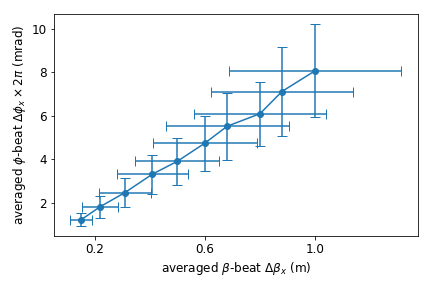
Figure 2: The correlation of $\beta_{x}$ and $\phi_{x}$ distortion distribution for the NSLS-II ring. This correlated distribution is calculated with the lattice model and could be used as another prior probability to eliminate incoherent measurement data. The farther away from the line, the less reliable the measured data is. Once a data point is not within the range of the error bars, it should be removed from the data pool.

Both $\beta$ and $\phi$-functions at different locations have different sensitivities to the quadrupole errors Courant and Snyder (1958). With a designed lattice model, one can compute another prior probability to specify different weights for each term in Eq. (9) and (14) to further optimize the algorithm. This process might be necessary for collider rings because the variation of $\beta$ is extremely large around interaction points, i.e., the final focus sections.

IV resolving degeneracy

In the previous section, we discussed the case in which the lattice distortion is due to normally distributed quadrupole errors. Once a real error is localized in a particular quadrupole, it may require us to identify which quadrupole is the root cause. This is nontrivial because quadrupoles are closely packed in modern storage rings, the NSLS-II being no exception. Therefore, their lattice response vectors (corresponding columns in $\boldsymbol{M}$) are often highly degenerated, especially between neighboring quadrupoles. The degeneracy between the $i^{th}$ and $j^{th}$ quadrupole is defined by the correlation coefficient Huang et al. (2007)

$$C_{i,j}=\frac{\boldsymbol{m}_{i}\cdot\boldsymbol{m}_{j}}{\|\boldsymbol{m}_{i}\|\;\|\boldsymbol{m}_{j}\|},$$ (17)

where $\boldsymbol{m}_{i}$ is the $i^{th}$ column of $\boldsymbol{M}$, which has $N$ elements. If $|C_{i,j}|$ approaches 1, it is difficult to distinguish which one is the actual error source with a full Jacobian matrix. It was found that rather than using all BPMs, and instead selecting a few specific BPMs among them, the highly degenerated quadrupoles were distinguishable.

Consider that there are $N$ BPMs. The $\beta$-beats seen by these BPMs are $N$-dimension vectors. Among them, $n\;(n\ll N)$ components can be selected to form two much shorter sub-vectors $\boldsymbol{v}_{i,j}$ in a such way that $\boldsymbol{v}_{i,j}$ have much less correlation between them. This means they should be as near-orthogonal as possible in an $n$ dimensional vector space. There are $N!/(n!(N-n)!)$ different permutations to select from. We found that it is not difficult to distinguish 5-6 BPMs out of 180 BPMs in the NSLS-II ring even if the correlation between some neighboring quadrupoles is above 0.98. Experimentally, we repetitively measure the lattice functions. Then we compute the correlation coefficients between $\boldsymbol{v}_{i,j}$ and the measured lattice distortion patterns, $\boldsymbol{u}$, as seen only at those 5-6 specific BPMs. If the quadrupole error was due to the $i^{th}$ quadrupole, the correlation coefficients $C_{v_{i},u}=\frac{\boldsymbol{v}_{i}\cdot\boldsymbol{u}}{\|\boldsymbol{v}_{i}\|\;\|\boldsymbol{u}\|}$ should be distributed close to $\pm 1$. Another one, $C_{v_{j},u}=\frac{\boldsymbol{v}_{j}\cdot\boldsymbol{u}}{\|\boldsymbol{v}_{j}\|\;\|\boldsymbol{u}\|}$ should be around zero, and vice versa.

To verify this technique, an experiment and a simulation study were carried out on the NSLS-II ring. The excitation current of one quadrupole QL1G2C01A (with an index of 10) was changed by 1 Ampere. The bunch-by-bunch feedback system Cheng et al. (2018) was then used to resonantly drive the beam to perform betatron oscillation at a nearly constant amplitude. Beam TbT data was acquired for $800\times 1024$ turns. For every 1024 turns of data, a set of $\beta_{x}$ functions was extracted at 180 BPMs. After averaging them, an error distribution was fitted out with the Bayesian approach. It was found that the maximum error is not QL1G2C01A as it should be, but its neighbor QL2G2C01A (with an index 11) (see Fig. 3). It is not surprising because the correlation between the $10^{th}$ and $11^{th}$ columns of the Jacobian $\boldsymbol{M}$ is as high as 0.9896.

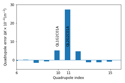
Figure 3: The $10^{th}$ quadrupole QL1G2C01A excitation is changed by 1 Ampere intentionally at the NSLS-II ring. By observing $\beta_{x}$ distortion at all 180 BPMs, the error source is incorrectly identified as its neighbor, the $11^{th}$ quadrupole QL2G2C01A. The reason for that is the correlation between the two magnets, as seen by all 180 BPMs, is as high as 0.9896.

Among 180 BPMs, we specifically selected 6 of them with their indices as {30, 31, 37, 62, 71, 78}. Observed at these BPMs, the unit $\beta_{x}$ functions response to these two quadrupoles is near-orthogonal with a correlation coefficient as low as 0.0612 (see Fig. 4). 800 independently measured $\beta_{x}$-beat patterns at those specific 6 BPMs were compared against these two unit response vectors $\boldsymbol{v}_{10,11}$. The histograms of their correlation coefficients are illustrated in Fig. 5. It becomes clear that the $\beta_{x}$ distortion is likely due to the quadrupole QL1G2C01A rather than its neighbor QL2G2C01A, because the measured optics distortion pattern is highly correlated with its response vector. A simulation was also performed to reproduce the experiment observation as illustrated in Fig. 6.

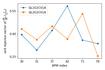
Figure 4: The unit $\beta_{x}$ responses vectors of quadrupole 10 and 11 seen at 6 selected BPMs. They are near-orthogonal in the 6-D vector space because their correlation calculated with Eq. (17) is as low as 0.0612.

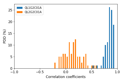
Figure 5: The probability density distribution (PDD) of the correlation coefficients between 800 measured $\beta_{x}$ distortion and two unit vectors $\boldsymbol{v}_{10,11}$. The independently and repeatedly measured $\beta$-beats are highly correlated with quadrupole 10’s pattern, rather than its neighbor. Based on that we can conclude that the actual error source is more likely from the quadrupole 10 (QL1G2C01A) instead of quadrupole 11 (QL2G2C01A).

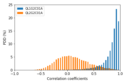
Figure 6: The probability density distribution (PDD) of the correlation coefficients between 25,000 simulated $\beta_{x}$-beats patterns and two unit vectors $\boldsymbol{v}_{10,11}$. The reproducibility further confirms our experiment observation.

V summary

The Bayesian approach explicitly emphasizes the coherence in the existing methods for linear lattice correction. By representing the lattice models as several likelihood functions and some prior probability distributions, overfitting of the optics corrections can be prevented. Prior probabilities can be calculated based on the lattice model prior to lattice correction. At the same time, the Bayesian approach gives the weights for different fitting objectives based on their measurement errors so that no objectives are over-emphasized by sacrificing others. If a distorted $\beta$ pattern comes from a single error source that is highly degenerated with its neighbors, it can be difficult to address. A new technique for resolving degeneracy and identifying the real error source has been demonstrated with both simulation and experimental observation.

The Bayesian approach is general and can be incorporated into other lattice and orbit correction algorithms or online optimizations McIntire et al. (2016), such as the linear optics from closed orbits (LOCO) algorithm Safranek (1997). The distortions of orbit response matrix (ORM) elements, due to each individual quadrupole error, can be calculated in advance and used to explicitly define the regularization coefficient to control overfitting Huang et al. (2007). Using a few specific ORM elements to compose orthogonal vectors should be able to address quadrupole degeneracy as well. One advantage of LOCO is that it unifies the $\beta$ and $\phi$ as the directly measurable parameters with their intrinsic correlation. Therefore, the fitting needs to be driven by a complete lattice model, and might be time-consuming. In some scenarios, the prolonged time the LOCO method would require may be considered worth it. For example, when TbT data is polluted by the beam decoherence due to a large positive chromaticity and/or nonlinearity Meller et al. (1987).