Computation of the analytic center of the solution set of the linear matrix inequality arising in continuous- and discrete-time passivity analysis

Abstract

In this paper formulas are derived for the analytic center of the solution set of linear matrix inequalities (LMIs) defining passive transfer functions. The algebraic Riccati equations that are usually associated with such systems are related to boundary points of the convex set defined by the solution set of the LMI. It is shown that the analytic center is described by closely related matrix equations, and their properties are analyzed for continuous- and discrete-time systems. Numerical methods are derived to solve these equations via steepest ascent and Newton-like methods. It is also shown that the analytic center has nice robustness properties when it is used to represent passive systems. The results are illustrated by numerical examples.

Keywords: Linear matrix inequality, analytic center, passivity, robustness, positive real system, algebraic Riccati equation
AMS Subject Classification: 93D09, 93C05, 49M15, 37J25

1 Introduction

We consider realizations of linear dynamical systems that are denoted as positive real or passive and their associated transfer functions. In particular, we study positive transfer functions which play a fundamental role in systems and control theory: they represent e. g., spectral density functions of stochastic processes, show up in spectral factorizations, are the Hermitian part of a positive real transfer function, characterize port-Hamiltonian systems, and are also related to algebraic Riccati equations.

Positive transfer functions form a convex set, and this property has lead to the extensive use of convex optimization techniques in this area (especially for so-called linear matrix inequalities [5]). In order to optimize a certain scalar function $f(X)$ over a convex set, one often defines a barrier function $b(X)$ that becomes infinite near the boundary of the set, and then finds the minimum of $c\cdot f(X)+b(X)$, $c\succeq 0$, as $c\rightarrow+\infty$. These minima (which are functions of the parameter $c$) are called the points of the central path. The starting point of this path ($c=0$) is called the analytic center of the set.

In this paper we present an explicit set of equations that define the analytic center of the solution set of the linear matrix inequality defining a passive transfer function. We also show how these equations relate to the algebraic Riccati equations that typically arise in the spectral factorization of transfer functions. We discuss transfer functions both on the imaginary axis (i. e. the continuous-time case), as well as on the unit circle (i. e. the discrete-time case). In the continuous-time setting the transfer function arises from the Laplace transform of the system

$$\begin{array}[]{rcl}\dot{x}&=&Ax+Bu,\ x(0)=0,\\ y&=&Cx+Du,\end{array}$$ (1)

where $u:\mathbb{R}\to\mathbb{C}^{m}$, $x:\mathbb{R}\to\mathbb{C}^{n}$, and $y:\mathbb{R}\to\mathbb{C}^{m}$ are vector-valued functions denoting, respectively, the input, state, and output of the system. Denoting real and complex $n$-vectors ($n\times m$ matrices) by $\mathbb{R}^{n}$, $\mathbb{C}^{n}$ ($\mathbb{R}^{n\times m}$, $\mathbb{C}^{n\times m}$), respectively, the coefficient matrices satisfy $A\in\mathbb{C}^{n\times n}$, $B\in\mathbb{C}^{n\times m}$, $C\in\mathbb{C}^{m\times n}$, and $D\in\mathbb{C}^{m\times m}$.

In the discrete-time setting the transfer function arises from the z-transform applied to the system

$$\begin{array}[]{rcl}x_{k+1}&=&Ax_{k}+Bu_{k},\ x_{0}=0,\\ y_{k}&=&Cx_{k}+Du_{k},\end{array}$$ (2)

with state, input, and output sequences $\{x_{k}\}$, $\{u_{k}\}$, $\{y_{k}\}$. In both cases, we usually denote these systems by four-tuples of matrices ${\mathcal{M}}:=\left\{A,B,C,D\right\}$ and the associated transfer functions by

$$\mathcal{T}_{c}(s):=D+C(sI_{n}-A)^{-1}B,\qquad\mathcal{T}_{d}(z):=D+C(zI_{n}-A)^{-1}B,$$ (3)

respectively.

We restrict ourselves to systems which are minimal, i. e. the pair $(A,B)$ is controllable (for all $\lambda\in\mathbb{C}$, $\operatorname{rank}\mbox{\small$[\,\lambda I-A\ B\,]$}=n$), and the pair $(A,C)$ is reconstructable (i. e. $(A^{\mathsf{H}},C^{\mathsf{H}})$ is controllable). Here, the conjugate transpose (transpose) of a vector or matrix $V$ is denoted by $V^{\mathsf{H}}$ ($V^{\mathsf{T}}$) and the identity matrix is denoted by $I_{n}$ or $I$ if the dimension is clear. We furthermore require that input and output port dimensions are equal to $m$ and assume that $\operatorname{rank}B=\operatorname{rank}C=m$.

Passive systems and their relationships with positive-real transfer functions are well studied, starting with the works [13, 17, 20, 21, 22, 23] and the topic has recently received a revival in the work on port-Hamiltonian (pH) systems, [18, 19]. For a summary of the relationships see [2, 20], where also the characterization of passivity via the solution set of an associated linear matrix inequality (LMI) is highlighted.

The paper is organized as follows. After some preliminaries in Section 2, in Section 3 we study the analytic centers of the solution sets of LMIs associated with the continuous- and discrete-time case. In Section 4 we discuss numerical methods to compute the analytic centers using steepest ascent as well as Newton-like methods and show that the analytic centers can be computed efficiently. In Section 5 lower bounds for the distance to non-passivity (the passivity radius) are derived using smallest eigenvalues of the Hermitian matrices associated with the linear matrix inequalities evaluated at the analytic center. The results are illustrated with some simple examples where the analytic center can be calculated analytically. In Appendix A we derive formulas for the computation of the gradients and the Hessian of the functions that we optimize and in Appendix B we clarify some of the differences that arise between the continuous- and the discrete-time case.

2 Preliminaries

Throughout this article we will use the following notation. We denote the set of Hermitian matrices in $\mathbb{C}^{n\times n}$ by ${\mathbb{H}_{n}}$. Positive definiteness (semidefiniteness) of $A\in{\mathbb{H}_{n}}$ is denoted by $A\succ 0$ ($A\succeq 0$). The real and imaginary parts of a complex matrix $Z$ are written as $\Re(Z)$ and $\Im(Z)$, respectively, and $\imath$ is the imaginary unit. We consider functions over ${\mathbb{H}_{n}}$, which is a vector space if considered as a real subspace of $\mathbb{R}^{\IfSubStr{n}{+}{(n)}{n}\times\IfSubStr{n}{+}{(n)}{n}}+\imath\mathbb{R}^{\IfSubStr{n}{+}{(n)}{n}\times\IfSubStr{n}{+}{(n)}{n}}$. We will identify $\mathbb{C}^{\IfSubStr{m}{+}{(m)}{m}\times\IfSubStr{n}{+}{(n)}{n}}$ with $\mathbb{R}^{\IfSubStr{m}{+}{(m)}{m}\times\IfSubStr{n}{+}{(n)}{n}}+\imath\mathbb{R}^{\IfSubStr{m}{+}{(m)}{m}\times\IfSubStr{n}{+}{(n)}{n}}$, but we note that this has implications when one is carrying out differentiations, see Appendix A. The Frobenius scalar product for matrices $X,Y\in\mathbb{R}^{\IfSubStr{n}{+}{(n)}{n}\times\IfSubStr{n}{+}{(n)}{n}}+\imath\mathbb{R}^{\IfSubStr{n}{+}{(n)}{n}\times\IfSubStr{n}{+}{(n)}{n}}$ is given by

$$\left\langle X,\,Y\right\rangle_{\mathbb{R}}:=\Re(\operatorname{tr}(A^{\mathsf{H}}B))=\operatorname{tr}(Y_{r}^{T}X_{r}+Y_{i}^{T}X_{i}),$$ (4)

where we have partitioned $X,Y$ as $X=X_{r}+\imath X_{i}$, $Y=Y_{r}+\imath Y_{i}$ with real and imaginary parts in $\mathbb{R}^{n\times n}$. As we are mainly concerned with this scalar product, we will drop the subscript $\mathbb{R}$. We will make frequent use of the following properties of this inner product given by

$$\left\langle X,\,Y\right\rangle=\left\langle Y,\,X\right\rangle,\,\|X\|_{F}=\left\langle X,\,X\right\rangle^{\frac{1}{2}},\,\left\langle X,\,YZ\right\rangle=\left\langle Y^{\mathsf{H}}X,\,Z\right\rangle=\left\langle XZ^{\mathsf{H}},\,Y\right\rangle.$$ (5)

The concepts of positive-realness and passivity are well studied. In the following subsections we briefly recall some important properties following [10, 20], where we repeat a few observations from [2]. See also [20] for a more detailed survey.

2.1 Positive-realness and passivity, continuous-time

Consider a continuous-time system ${\mathcal{M}}$ as in (1) and the transfer function $\mathcal{T}_{c}$ as in (3). The transfer function $\mathcal{T}_{c}(s)$ is called positive real if the matrix-valued rational function

$$\Phi_{c}(s):=\mathcal{T}_{c}^{\mathsf{H}}(-s)+\mathcal{T}_{c}(s)$$

is positive semidefinite for $s$ on the imaginary axis, i. e. $\Phi_{c}(\imath\omega)\succeq 0$ for all $\omega\in\mathbb{R}$ and it is called strictly positive real if $\Phi_{c}(\imath\omega)\succ 0$ for all $\ \omega\in\mathbb{R}$.

We associate with $\Phi_{c}$ a system pencil

$$S_{c}(s):=\left[\begin{array}[]{cc|c}0&A-sI_{n}&B\\ A^{\mathsf{H}}+sI_{n}&0&C^{\mathsf{H}}\\ \hline\cr B^{\mathsf{H}}&C&R\end{array}\right],$$ (6)

where $R:=D+D^{\mathsf{H}}$. Here (6) has a Schur complement which is the transfer function $\Phi_{c}(s)$ and the generalized eigenvalues of $S_{c}(s)$ are the zeros of $\Phi_{c}(s)$.

For $X\in{\mathbb{H}_{n}}$ we introduce the matrix function

$$W_{c}(X):=\left[\begin{array}[]{cc}-X\,A-A^{\mathsf{H}}X&C^{\mathsf{H}}-X\,B\\ C-B^{\mathsf{H}}X&D+D^{\mathsf{H}}\end{array}\right],$$ (7)

If $\mathcal{T}_{c}(s)$ is positive real, then the linear matrix inequality (LMI)

$$W_{c}(X)\succeq 0$$ (8)

has a solution $X\in{\mathbb{H}_{n}}$ and we have the sets

$${\mathbb{X}_{c}^{\raisebox{1.39998pt}{{$\succ$}}}}:=\left\{X\in{\mathbb{H}_{n}}\left|W_{c}(X)\succeq 0,\ X\succ 0\right.\right\},$$ (9a)

$${\mathbb{X}_{c}^{\raisebox{1.39998pt}{{$\ggcurly$}}}}:=\left\{X\in{\mathbb{H}_{n}}\left|W_{c}(X)\succ 0,\ X\succ 0\right.\right\}.$$ (9b)

An important subset of ${\mathbb{X}_{c}^{\raisebox{1.39998pt}{{$\succ$}}}}$ are those solutions to (8) for which the rank $r$ of $W_{c}(X)$ is minimal (i. e.  for which $r=\operatorname{rank}\Phi_{c}(s)$). If $R$ is invertible, then the minimum rank solutions in ${\mathbb{X}_{c}^{\raisebox{1.39998pt}{{$\succ$}}}}$ are those for which $\operatorname{rank}W_{c}(X)=\operatorname{rank}(R)=m$, which in turn is the case if and only if the Schur complement of $R$ in $W_{c}(X)$ is zero. This Schur complement is associated with the continuous-time algebraic Riccati equation (ARE)

$$\mathsf{Ricc}_{c}(X):=-XA-A^{\mathsf{H}}X-(C^{\mathsf{H}}-XB)R^{-1}(C-B^{\mathsf{H}}X)=0.$$ (10)

Solutions $X$ to (10) produce a spectral factorization of $\Phi_{c}(s)$, and each solution corresponds to a Lagrangian invariant subspace spanned by the columns of $U_{c}:=\left[\begin{array}[]{cc}I_{n}&-X^{\mathsf{T}}\end{array}\right]^{\mathsf{T}}$ that remains invariant under the action of the Hamiltonian matrix

$${\mathcal{H}}_{c}:=\left[\begin{array}[]{cc}A-BR^{-1}C&-BR^{-1}B^{\mathsf{H}}\\ C^{\mathsf{H}}R^{-1}C&-(A-BR^{-1}C)^{\mathsf{H}}\end{array}\right],$$ (11)

i. e. $U_{c}$ satisfies ${\mathcal{H}}_{c}U_{c}=U_{c}A_{F_{c}}$ for a closed loop matrix $A_{F_{c}}=A-BF_{c}$ with $F_{c}:=R^{-1}(C-B^{\mathsf{H}}X)$ (see e.g., [8]). Each solution $X$ of (10) can also be associated with an extended Lagrangian invariant subspace for the pencil $S_{c}(s)$ (see [4]), spanned by the columns of $\widehat{U}_{c}:=\left[\begin{array}[]{ccc}-X^{\mathsf{T}}&I_{n}&-F_{c}^{\mathsf{T}}\end{array}\right]^{\mathsf{T}}$. In particular, $\widehat{U}_{c}$ satisfies

$$\left[\begin{array}[]{ccc}0&A&B\\ A^{\mathsf{H}}&0&C^{\mathsf{H}}\\ B^{\mathsf{H}}&C&R\end{array}\right]\widehat{U}_{c}=\left[\begin{array}[]{ccc}0&I_{n}&0\\ -I_{n}&0&0\\ 0&0&0\end{array}\right]\widehat{U}_{c}A_{F_{c}}.$$

The sets ${\mathbb{X}_{c}^{\raisebox{1.39998pt}{{$\succ$}}}},{\mathbb{X}_{c}^{\raisebox{1.39998pt}{{$\ggcurly$}}}}$ are related to the concepts of passivity and strict passivity see [20]. If for the system ${\mathcal{M}}:=\left\{A,B,C,D\right\}$ of (6) the LMI (8) has a solution $X\in{\mathbb{X}_{c}^{\raisebox{1.39998pt}{{$\succ$}}}}$ then ${\mathcal{M}}$ is (Lyapunov) stable (i.e. all eigenvalues are in the closed left half plane with any eigenvalues occurring on the imaginary axis being semisimple), and passive, and if there exists a solution $X\in{\mathbb{X}_{c}^{\raisebox{1.39998pt}{{$\ggcurly$}}}}$ then ${\mathcal{M}}$ is asymptocially stable, (i.e. all eigenvalues are the open left half plane) and strictly passive. Furthermore, if ${\mathcal{M}}$ is passive, then there exist maximal and minimal solutions $X_{-}\preceq X_{+}$ of (8) in ${\mathbb{X}_{c}^{\raisebox{1.39998pt}{{$\succ$}}}}$ such that all solutions $X$ of $W_{c}(X)\succeq 0$ satisfy

$$0\prec X_{-}\preceq X\preceq X_{+},$$

which implies that ${\mathbb{X}_{c}^{\raisebox{1.39998pt}{{$\succ$}}}}$ is bounded. For more details on the different concepts discussed in this section, see [2].

2.2 Positive-realness and passivity, discrete-time

For each of the results of the previous subsection there are discrete-time versions which we briefly recall in this section, see [12, 17]. Note, that these results can be obtained by applying a bilinear transform (see Appendix B) to the continuous-time counterparts.

The transfer function $\mathcal{T}_{d}(s)$ in (3) is called positive real if the matrix-valued rational function

$$\Phi_{d}(z):=\mathcal{T}_{d}^{\mathsf{H}}(z^{-1})+\mathcal{T}_{d}(z)$$

satisfies $\Phi_{d}(e^{\imath\omega})=\Phi_{d}^{\mathsf{H}}(e^{\imath\omega})\succeq 0$ for $0\leq\omega\leq 2\pi$, and it is called strictly positive real if $\Phi_{d}(e^{\imath\omega})\succ 0$ for $0\leq\omega\leq 2\pi$.

We consider an associated the matrix function

$$W_{d}(X)=\left[\begin{array}[]{cc}X-A^{\mathsf{H}}X\,A&C^{\mathsf{H}}-A^{\mathsf{H}}X\,B\\ C-B^{\mathsf{H}}X\,A&B^{\mathsf{H}}X\,B+R\end{array}\right],$$ (12)

where again $R=D+D^{\mathsf{H}}$, the sets

$${\mathbb{X}_{d}^{\raisebox{1.39998pt}{{$\succ$}}}}:=\left\{X\in{\mathbb{H}_{n}}\left|W_{d}(X)\succeq 0,\ X\succ 0\right.\right\},$$ (13a)

$${\mathbb{X}_{d}^{\raisebox{1.39998pt}{{$\ggcurly$}}}}:=\left\{X\in{\mathbb{H}_{n}}\left|W_{d}(X)\succ 0,\ X\succ 0\right.\right\}.$$ (13b)

and the system pencil

$$S_{d}(z)=\left[\begin{array}[]{cc|c}0&A-zI_{n}&B\\ zA^{\mathsf{H}}-I_{n}&0&C^{\mathsf{H}}\\ \hline\cr zB^{\mathsf{H}}&C&R\end{array}\right]$$ (14)

whose Schur complement is $\Phi_{d}(z)$.

If the system is positive real then, see [20], there exists $X\in{\mathbb{H}_{n}}$ such that $W_{d}(X)\succeq 0$. If that is the case, a transfer function ${\mathcal{T}}_{d}(z):=C(zI_{n}-A)^{-1}B+D$ is called passive and strictly passive if even $W_{d}(X)\succ 0$. We again have an associated discrete-time Riccati equation defined as

$$\mathsf{Ricc}_{d}(X):=-A^{\mathsf{H}}XA+X-(C^{\mathsf{H}}-A^{\mathsf{H}}XB)(R-B^{\mathsf{H}}XB)^{-1}(C-B^{\mathsf{H}}XA)=0.$$ (15)

from which one directly obtains a spectral factorization of $\Phi_{d}(z)$. The solutions of the discrete-time Riccati equation can be obtained by computing a Lagrangian invariant subspace spanned by the columns of $U_{d}:=\left[\begin{array}[]{cc}I_{n}&-X^{\mathsf{T}}\end{array}\right]^{\mathsf{T}}$ of the symplectic matrix

$${\mathcal{S}}_{d}:=\left[\begin{array}[]{cc}I&BR^{-1}B^{\mathsf{H}}\\ 0&A^{\mathsf{H}}-C^{\mathsf{H}}R^{-1}B^{\mathsf{H}}\end{array}\right]^{-1}\left[\begin{array}[]{cc}A-BR^{-1}C&0\\ C^{\mathsf{H}}R^{-1}C&I\end{array}\right],$$

satisfying ${\mathcal{S}}_{d}U_{d}=U_{d}A_{F_{d}}$, where $A_{F_{d}}:=A-BF_{d}$ with $F_{d}:=(R-B^{\mathsf{H}}XB)^{-1}(C-B^{\mathsf{H}}XA)$.

Each solution $X$ of (15) can also be associated with an extended Lagrangian invariant subspace for the pencil $S_{d}(z)$ (see [4]), spanned by the columns of $\widehat{U}_{d}:=\left[\begin{array}[]{ccc}-X^{\mathsf{T}}&I_{n}&-F_{d}^{\mathsf{T}}\end{array}\right]^{\mathsf{T}}$. In particular, $\widehat{U}_{d}$ satisfies

$$\left[\begin{array}[]{ccc}0&A&B\\ I_{n}&0&C^{\mathsf{H}}\\ 0&C&R\end{array}\right]\widehat{U}_{d}=\left[\begin{array}[]{ccc}0&I_{n}&0\\ A^{\mathsf{H}}&0&0\\ B^{\mathsf{H}}&0&0\end{array}\right]\widehat{U}_{d}A_{F_{d}}.$$

Again, if the system is passive, then there exist maximal and minimal solutions $X_{-}\preceq X_{+}$ in ${\mathbb{X}_{d}^{\raisebox{1.39998pt}{{$\ggcurly$}}}}$, such that all solutions $X$ of $W_{d}(X)\succeq 0$ satisfy

$$0\prec X_{-}\preceq X\preceq X_{+},$$

which implies that ${\mathbb{X}_{d}^{\raisebox{1.39998pt}{{$\succ$}}}}$ is bounded.

3 The analytic center

If the sets ${\mathbb{X}_{c}^{\raisebox{1.39998pt}{{$\ggcurly$}}}}$, ${\mathbb{X}_{d}^{\raisebox{1.39998pt}{{$\ggcurly$}}}}$ in (9), respectively (13), are non-empty, then we can define their respective analytic center. Following the discussion in [10], we first consider the continuous-time case, the discrete-time case is derived in an analogous way. We choose a scalar barrier function

$$b(X):=-\ln\det W_{c}(X),$$ (16)

which is bounded from below but becomes infinitely large when $W_{c}(X)$ becomes singular. We define the analytic center of the domain ${\mathbb{X}_{c}^{\raisebox{1.39998pt}{{$\ggcurly$}}}}$ as the minimizer of this barrier function.

3.1 The continuous-time case

The solutions $X_{+}$ and $X_{-}$ of the Riccati equation $\mathsf{Ricc}_{c}(X)=0$ in (10), are both on the boundary of ${\mathbb{X}_{c}^{\raisebox{1.39998pt}{{$\succ$}}}}$, and hence are not in ${\mathbb{X}_{c}^{\raisebox{1.39998pt}{{$\ggcurly$}}}}$. Since we assume that ${\mathbb{X}_{c}^{\raisebox{1.39998pt}{{$\ggcurly$}}}}$ is non-empty, the analytic center is well defined, see, e. g., , Section 4.2 in [16].

To characterize the analytic center, we first need to find a variation of the gradient $b_{X}$ of the barrier function $b$ at point $X$ along direction $\Delta_{X}$, which is equal to

$$\left\langle W_{c}(X)^{-1},\,\Delta W_{c}(X)[\Delta_{X}]\right\rangle,$$ (17)

where $b_{X}=W_{c}(X)^{-1}$ and $\Delta W_{c}(X)[\Delta_{X}]$ is the incremental step in the direction $\Delta_{X}$, for details see Appendix A. It appears that $X$ is an extremal point of the barrier function if and only if

$$\left\langle W_{c}(X)^{-1},\,\Delta W_{c}(X)[\Delta_{X}]\right\rangle=0\quad\text{for all }\Delta_{X}=\Delta_{X}^{\mathsf{H}}.$$ (18)

The increment of $W_{c}(X)$ corresponding to an incremental direction $\Delta_{X}=\Delta_{X}^{\mathsf{H}}$ of $X$ is given by

$$\Delta W_{c}(X)[\Delta_{X}]=-\left[\begin{array}[]{cc}A^{\mathsf{H}}\Delta_{X}+\Delta_{X}A&\Delta_{X}B\\ B^{\mathsf{H}}\Delta_{X}&0\end{array}\right].$$

The equation for the extremal point then becomes

$$\left\langle W_{c}(X)^{-1},\,\left[\begin{array}[]{cc}A^{\mathsf{H}}\Delta_{X}+\Delta_{X}A&\Delta_{X}B\\ B^{\mathsf{H}}\Delta_{X}&0\end{array}\right]\right\rangle=0\quad\text{for all }\Delta_{X}=\Delta_{X}^{\mathsf{H}}.$$ (19)

Defining

$$F_{c}:=R^{-1}(C-B^{\mathsf{H}}X),\quad P_{c}:=-A^{\mathsf{H}}X-XA-F_{c}^{\mathsf{H}}RF_{c},$$

then

$$W_{c}(X)=\left[\begin{array}[]{cc}I&F_{c}^{\mathsf{H}}\\ 0&I\end{array}\right]\left[\begin{array}[]{cc}P_{c}&0\\ 0&R\end{array}\right]\left[\begin{array}[]{cc}I&0\\ F_{c}&I\end{array}\right].$$

For a point $X\in{\mathbb{X}_{c}^{\raisebox{1.39998pt}{{$\ggcurly$}}}}$ it is obvious that we also have $P_{c}=\mathsf{Ricc}_{c}(X)\succ 0$, and hence (19) is equivalent to

$$\left\langle\left[\begin{array}[]{cc}P_{c}^{-1}&0\\ 0&R^{-1}\end{array}\right],\,\left[\begin{array}[]{cc}I&-F_{c}^{\mathsf{H}}\\ 0&I\end{array}\right]\left[\begin{array}[]{cc}A^{\mathsf{H}}\Delta_{X}+\Delta_{X}A&\Delta_{X}B\\ B^{\mathsf{H}}\Delta_{X}&0\end{array}\right]\left[\begin{array}[]{cc}I&0\\ -F_{c}&I\end{array}\right]\right\rangle=0,$$

or

$$\left\langle P_{c}^{-1},\,A^{\mathsf{H}}\Delta_{X}+\Delta_{X}A-F_{c}^{\mathsf{H}}B^{\mathsf{H}}\Delta_{X}-\Delta_{X}BF_{c}\right\rangle=0,$$

and this is equivalent to

$$P_{c}^{-1}A_{F_{c}}^{\mathsf{H}}+A_{F_{c}}P_{c}^{-1}=0,$$ (20)

where we have set $A_{F_{c}}=A-BF_{c}$.

We emphasize that $P_{c}$ is nothing but the Riccati operator $\mathsf{Ricc}_{c}(X)$ defined in (10), and that $A_{F_{c}}$ is the corresponding closed loop matrix. For the classical Riccati solutions we have $P_{c}=\mathsf{Ricc}_{c}(X)=0$ and the corresponding closed loop matrix is well-known to have its eigenvalues equal to a subset of the eigenvalues of the corresponding Hamiltonian matrix (11).

Since $P_{c}=\mathsf{Ricc}_{c}(X)\succ 0$, it follows that $P_{c}$ has a Hermitian square root $T_{c}$ satisfying $P_{c}=T_{c}^{2}$. Transforming (20) with the invertible matrix $T_{c}$, we obtain

$$T_{c}^{-1}A_{F_{c}}^{\mathsf{H}}T_{c}+T_{c}A_{F_{c}}T_{c}^{-1}=0.$$

Hence $\hat{A}_{F_{c}}:=T_{c}A_{F_{c}}T_{c}^{-1}$ is skew-Hermitian and has all its eigenvalues on the imaginary axis, and so does $A_{F_{c}}$. Therefore, the closed loop matrix $A_{F_{c}}$ of the analytic center has a spectrum that is also central.

It is important to also note that

$$\det W_{c}(X)=\det\mathsf{Ricc}_{c}(X)\det R,$$

which implies that we are also finding a stationary point of $\det\mathsf{Ricc}_{c}(X)$, since $\det R$ is constant and non-zero.

Since the matrix $P_{c}$ is positive definite and invertible, we can rewrite the equations defining the analytic center as

$$RF_{c} =C-B^{\mathsf{H}}X,$$ (21a)

$$P_{c} =-A^{\mathsf{H}}X-XA-F_{c}^{\mathsf{H}}RF_{c},$$ (21b)

$$0 =P_{c}(A-BF_{c})+(A^{\mathsf{H}}-F_{c}^{\mathsf{H}}B^{\mathsf{H}})P_{c},$$ (21c)

where $X=X^{\mathsf{H}}$ and $P_{c}=P_{c}^{\mathsf{H}}\succ 0$. We can compute the analytic center by solving these three equations which actually form a cubic equation in $X$.

Note that even though the eigenvalues of the closed loop matrix $F_{c}$ associated with the analytic center are all purely imaginary, the eigenvalues of the original system and the poles of the transfer function stay invariant under the state space transformation $\mathcal{T}_{c}$.

3.2 The discrete-time case

For discrete-time systems, the increment of $W_{d}(X)$ equals

$$\Delta W_{d}(X)[\Delta_{X}]=-\left[\begin{array}[]{cc}A^{\mathsf{H}}\Delta_{X}A-\Delta_{X}&A^{\mathsf{H}}\Delta_{X}B\\ B^{\mathsf{H}}\Delta_{X}A&B^{\mathsf{H}}\Delta_{X}B\end{array}\right],$$ (22)

for all $\Delta_{X}=\Delta_{X}^{\mathsf{H}}$. Defining $F_{d}:=(R-B^{\mathsf{H}}XB)^{-1}(C-B^{\mathsf{H}}XA)$, $P_{d}:=-A^{\mathsf{H}}XA+X-F_{d}^{\mathsf{H}}(R-B^{\mathsf{H}}XB)F_{d}$, and $A_{F_{d}}:=A-BF_{d}$, then $W_{d}(X)$ factorizes as

$$W_{d}(X)=\left[\begin{array}[]{cc}I&F_{d}^{\mathsf{H}}\\ 0&I\end{array}\right]\left[\begin{array}[]{cc}P_{d}&0\\ 0&R-B^{\mathsf{H}}XB\end{array}\right]\left[\begin{array}[]{cc}I&0\\ F_{d}&I\end{array}\right],$$ (23)

and the equation for the extremal point becomes

$$\Bigg{\langle}\left[\begin{array}[]{cc}P_{d}^{-1}&0\\ 0&(R-B^{\mathsf{H}}XB)^{-1}\end{array}\right],$$ (26)

$$\qquad\left[\begin{array}[]{cc}I&-F_{d}^{\mathsf{H}}\\ 0&I\end{array}\right]\left[\begin{array}[]{cc}A^{\mathsf{H}}\Delta_{X}A-\Delta_{X}&A^{\mathsf{H}}\Delta_{X}B\\ B^{\mathsf{H}}\Delta_{X}A&B^{\mathsf{H}}\Delta_{X}B\end{array}\right]\left[\begin{array}[]{cc}I&0\\ -F_{d}&I\end{array}\right]\Bigg{\rangle}=0,$$ (33)

or

$$\left\langle P_{d}^{-1},\,A_{F_{d}}^{\mathsf{H}}\Delta_{X}A_{F_{d}}-\Delta_{X}\right\rangle+\left\langle(R-B^{\mathsf{H}}XB)^{-1},\,B^{\mathsf{H}}\Delta_{X}B\right\rangle=0.$$ (34)

This is equivalent to

$$A_{F_{d}}P_{d}^{-1}A_{F_{d}}^{\mathsf{H}}-P_{d}^{-1}+B(R-B^{\mathsf{H}}XB)^{-1}B^{\mathsf{H}}=0,$$ (35)

which is a non-homogenous discrete-time Lyapunov equation. Since $(A,B)$ is controllable (by assumption), so is $(A_{F_{c}},B)$ and it follows then from (35) that the eigenvalues of $A_{F_{d}}$ are now strictly inside the unit circle. This is clearly different from the continuous-time case, where the spectrum of $A_{F_{c}}$ was on the boundary of the stability region. The equations defining the discrete-time analytic center then become

$$(R-B^{\mathsf{H}}XB)F_{d} =C-B^{\mathsf{H}}XA,$$ (36a)

$$P_{d} =C^{\mathsf{H}}R^{-1}C+X-A^{\mathsf{H}}XA$$

$$\qquad-F_{d}^{\mathsf{H}}(R-B^{\mathsf{H}}XB)F_{d},$$ (36b)

$$0 =(A-BF_{d})P_{d}^{-1}(A^{\mathsf{H}}-F_{d}^{\mathsf{H}}B^{\mathsf{H}})$$

$$\qquad-P_{d}^{-1}+B(R-B^{\mathsf{H}}XB)^{-1}B^{\mathsf{H}}.$$ (36c)

Remark 3.1.

Note that we could have transformed the solution of the corresponding continuous-time problem via a bilinear transform, which would then yield a feedback $F_{d}$ that puts all eigenvalues on the unit circle, but the feedback would of course be different. For a more detailed discussion, see Appendix B.

4 Numerical computation of the analytic center

In this section we present methods for the numerical computation of the analytic center.

Suppose that we are at a point $X_{0}\in{\mathbb{X}_{c}^{\raisebox{1.39998pt}{{$\ggcurly$}}}}\ ({\mathbb{X}_{d}^{\raisebox{1.39998pt}{{$\ggcurly$}}}})$ and want to perform the next step using an increment $\Delta_{X}$. We discuss a steepest ascent and a Newton-like method to obtain that increment.

4.1 A steepest ascent method

In order to formulate an optimization scheme to compute the analytic center, we can use the gradient of the barrier function $b(X)$ with respect to $X$ to obtain a steepest ascent method.

In the continuous-time case, we then need to take a step $\Delta_{X}$ for which $\left\langle b_{W}(X_{0}),\,\Delta W_{c}(X_{0})[\Delta_{X}]\right\rangle$ is maximal, which is equivalent to

$$\Delta_{X}:=\operatorname*{\arg\,\max}_{\left\langle\Delta_{X},\,\Delta_{X}\right\rangle=1}\left\langle P_{c}^{-1}(X_{0})A_{F_{c}}(X_{0})^{\mathsf{H}}+A_{F_{c}}(X_{0})P_{c}^{-1}(X_{0}),\,\Delta_{X}\right\rangle.$$

The maximum is obtained by choosing $\Delta_{X}$ proportional to the gradient

$$P_{c}^{-1}(X_{0})A_{F_{c}}(X_{0})^{\mathsf{H}}+A_{F_{c}}(X_{0})P_{c}^{-1}(X_{0}).$$

The corresponding optimal stepsize $\alpha$ for the increment $\Delta_{X}$ can be obtained from the determinant of the incremented LMI $W_{c}(X_{0}+\alpha\Delta_{X})\succ 0$.

In the discrete-time case, we obtain the increment from

$$\Delta_{X}:=$$ (37)

$$\quad\operatorname*{\arg\,\max}_{\left\langle\Delta_{X},\,\Delta_{X}\right\rangle=1}\left\langle A_{F_{d}}(X_{0})P_{d}^{-1}(X_{0})A_{F_{d}}^{\mathsf{H}}(X_{0})-P_{d}^{-1}(X_{0})+B(R-B^{\mathsf{H}}X_{0}B)^{-1}B^{\mathsf{H}},\,\Delta_{X}\right\rangle.$$ (38)

The maximum is obtained by choosing $\Delta_{X}$ proportional to

$$A_{F_{d}}(X_{0})P_{d}^{-1}(X_{0})A_{F_{d}}^{\mathsf{H}}(X_{0})-P_{d}^{-1}(X_{0})+B(R-B^{\mathsf{H}}X_{0}B)^{-1}B^{\mathsf{H}},$$

and the stepsize $\alpha$ for the increment $\Delta_{X}$ can again be obtained from the determinant of the incremented LMI $W_{d}(X_{0}+\alpha\Delta_{X})\succ 0$.

Remark 4.1.

The detailed explanation how to compute the stepsize $\alpha$ will be done later as a special case of the derivation of the Newton step, see subsection 4.2. The idea is to find the second order Taylor expansion of the function $f(X_{0}+\alpha\Delta_{X})=-\ln\det G(X_{0}+\alpha\Delta_{X})$ and then to maximize this quadratic function in the scalar $\alpha$.

4.2 A Newton-like method

For the computation of a Newton-like increment $\Delta_{X}$ we also need the Hessian of the barrier function $b$. In order to simplify the derivation we first equivalently reformulate the barrier function into a more suitable form.

4.2.1 The continuous-time case

In the continuous-time case, we have that

$$W_{c}(X_{0}+\Delta_{X})=\left[\begin{array}[]{cc}Q_{0}&C_{0}^{\mathsf{H}}\\ C_{0}&R_{0}\end{array}\right]-\left[\begin{array}[]{c}\Delta_{X}\\ 0\end{array}\right]\left[\begin{array}[]{cc}A&B\end{array}\right]-\left[\begin{array}[]{c}A^{\mathsf{H}}\\ B^{\mathsf{H}}\end{array}\right]\left[\begin{array}[]{cc}\Delta_{X}&0\end{array}\right],$$

where

$$\left[\begin{array}[]{cc}Q_{0}&C_{0}^{\mathsf{H}}\\ C_{0}&R_{0}\end{array}\right]:=W_{c}(X_{0}).$$

Up to the constant $(-1)^{n}$, the determinant of $W_{c}(X_{0}+\Delta_{X})$ is equal to

$$\det\left[\begin{array}[]{cc|cc}0&I_{n}&\Delta_{X}&0\\ I_{n}&0&A&B\\ \hline\cr\Delta_{X}&A^{\mathsf{H}}&Q_{0}&C_{0}^{\mathsf{H}}\\ 0&B^{\mathsf{H}}&C_{0}&R_{0}\end{array}\right]=\det\left[\begin{array}[]{cc|cc}0&I_{n}&\Delta_{X}&0\\ I_{n}&0&A_{F_{c}}&B\\ \hline\cr\Delta_{X}&A_{F_{c}}^{\mathsf{H}}&P_{0}&0\\ 0&B^{\mathsf{H}}&0&R_{0}\end{array}\right],$$ (39)

where $A_{F_{c}}:=A-BR_{0}^{-1}C_{0}$ and $P_{0}:=Q_{0}-C_{0}^{\mathsf{H}}R_{0}^{-1}C_{0}$ are associated with the current point $X_{0}$. Carrying out an additional congruence transformation with

$$Z_{c}:=\left[\begin{array}[]{cccc}P_{0}^{-\frac{1}{2}}&0&0&0\\ 0&P_{0}^{\frac{1}{2}}&0&-\hat{B}R_{0}^{-1}\\ 0&0&P_{0}^{-\frac{1}{2}}&0\\ 0&0&0&I_{m}\end{array}\right],$$

we obtain

$$\left[\begin{array}[]{cccc}0&I_{n}&\hat{\Delta}_{X}&0\\ I_{n}&-\hat{B}R_{0}^{-1}\hat{B}^{\mathsf{H}}&\hat{A}_{F_{c}}&0\\ \hat{\Delta}_{X}&\hat{A}_{F_{c}}^{\mathsf{H}}&I_{n}&0\\ 0&0&0&R_{0}\end{array}\right]:=Z_{c}\left[\begin{array}[]{cccc}0&I_{n}&\Delta_{X}&0\\ I_{n}&0&A_{F_{c}}&B\\ \Delta_{X}&A_{F_{c}}^{\mathsf{H}}&P_{0}&0\\ 0&B^{\mathsf{H}}&0&R_{0}\end{array}\right]Z_{c}^{\mathsf{H}},$$

where $\hat{B}=P_{0}^{\frac{1}{2}}B$, $\hat{A}_{F_{c}}:=P_{0}^{\frac{1}{2}}A_{F}P_{0}^{-\frac{1}{2}}$, and $\hat{\Delta}_{X}=P_{0}^{-\frac{1}{2}}\Delta_{X}P_{0}^{-\frac{1}{2}}$. It is clear that the determinant of the congruence transformation introduces a factor $\det(P_{0})$. Finally, the determinant of the transformed matrix is, up to a constant $\det(R_{0})$, equal to

$$\det\left[\begin{array}[]{cc}-\hat{\Delta}_{X}&I_{n}\end{array}\right]\left[\begin{array}[]{cc}-\hat{B}R_{0}^{-1}\hat{B}^{\mathsf{H}}&\hat{A}_{F_{c}}\\ \hat{A}_{F_{c}}^{\mathsf{H}}&I_{n}\end{array}\right]\left[\begin{array}[]{cc}-\hat{\Delta}_{X}\\ I_{n}\end{array}\right]\\ =\det\left[I_{n}-\hat{\Delta}_{X}\hat{A}_{F_{c}}-\hat{A}_{F_{c}}^{\mathsf{H}}\hat{\Delta}_{X}-\hat{\Delta}_{X}\hat{B}R_{0}^{-1}\hat{B}^{\mathsf{H}}\hat{\Delta}_{X}\right].$$ (40)

This is the multiplying factor of the current value of $\det W_{c}(X_{0})$ and we can make it larger than $1$ if $\hat{A}_{F_{c}}$ is not skew-Hermitian yet. Introduce

$$f(X) :=-\ln\det(G(X)),$$ (41)

$$Q_{c} :=\hat{B}R_{0}^{-1}\hat{B}^{\mathsf{H}},$$ (42)

$$G(X) :=I_{n}-X\hat{A}_{F_{c}}-\hat{A}_{F_{c}}^{\mathsf{H}}X-XQ_{c}X.$$ (43)

In the set of Hermitian matrices (over the reals), the gradient of $f(X)$ then is given by

$$f_{X}(X)[\Delta]=\langle-G(X)^{-1},-(\Delta\hat{A}_{F_{c}}+\hat{A}_{F_{c}}^{\mathsf{H}}\Delta+\Delta Q_{c}X+XQ_{c}\Delta)\rangle$$

and the Hessian is given by

$$f_{XX}(X)[\Delta,\Delta] =\left<-G(X)^{-1}(\Delta\hat{A}_{F_{c}}+\hat{A}_{F_{c}}^{\mathsf{H}}\Delta+\Delta Q_{c}X+XQ_{c}\Delta)G(X)^{-1},\right.$$ (44)

$$\qquad\left.-(\Delta\hat{A}_{F_{c}}+\hat{A}_{F_{c}}^{\mathsf{H}}\Delta+\Delta Q_{c}X+XQ_{c}\Delta)\right>$$ (45)

$$\qquad+\langle-G(X)^{-1},-2\Delta Q_{c}\Delta\rangle.$$ (46)

A second order approximation of $f$ (at $X=0$) is given by

$$f(\Delta)\approx T^{(2)}_{f}(\Delta) =f(0)+f_{X}(0)[\Delta]+\frac{1}{2}f_{XX}(0)[\Delta,\Delta]$$ (47)

$$=\langle I_{n},\Delta\hat{A}_{F_{c}}+\hat{A}_{F_{c}}^{\mathsf{H}}\Delta\rangle+\frac{1}{2}\langle\Delta\hat{A}_{F_{c}}+\hat{A}_{F_{c}}^{\mathsf{H}}\Delta,\Delta\hat{A}_{F_{c}}+\hat{A}_{F_{c}}^{\mathsf{H}}\Delta\rangle$$ (48)

$$\qquad+\langle I_{n},\Delta Q_{c}\Delta\rangle,$$ (49)

and we want the gradient of $f$ to be $0$. For the Newton step we want to determine $\Delta=\Delta^{\mathsf{H}}$ such that $\frac{\partial T^{(2)}_{f}}{\partial\Delta}(\Delta)=0$, i. e. we require that

$$\langle I_{n},Y\hat{A}_{F_{c}}+\hat{A}_{F_{c}}^{\mathsf{H}}Y\rangle+\langle\Delta\hat{A}_{F_{c}}+\hat{A}_{F_{c}}^{\mathsf{H}}\Delta,Y\hat{A}_{F_{c}}+\hat{A}_{F_{c}}^{\mathsf{H}}Y\rangle+2\langle I_{n},YQ_{c}\Delta\rangle=0$$ (50)

for all $Y=Y^{\mathsf{H}}$. Using the properties of the scalar product, we obtain that this is equivalent to

$$\langle Y,\hat{A}_{F_{c}}^{\mathsf{H}}+\hat{A}_{F_{c}}+\hat{A}_{F_{c}}\Delta\hat{A}_{F_{c}}+\hat{A}_{F_{c}}\hat{A}_{F_{c}}^{\mathsf{H}}\Delta+\hat{A}_{F_{c}}^{\mathsf{H}}\Delta\hat{A}_{F_{c}}^{\mathsf{H}}+\Delta\hat{A}_{F_{c}}\hat{A}_{F_{c}}^{\mathsf{H}}+Q_{c}\Delta+\Delta Q_{c}\rangle=0$$

for all $Y=Y^{\mathsf{H}}$, or equivalently

$$\hat{A}_{F_{c}}\Delta\hat{A}_{F_{c}}+\hat{A}_{F_{c}}\hat{A}_{F_{c}}^{\mathsf{H}}\Delta+\hat{A}_{F_{c}}^{\mathsf{H}}\Delta\hat{A}_{F_{c}}^{\mathsf{H}}+\Delta\hat{A}_{F_{c}}\hat{A}_{F_{c}}^{\mathsf{H}}+Q_{c}\Delta+\Delta Q_{c}=-\hat{A}_{F_{c}}^{\mathsf{H}}-\hat{A}_{F_{c}}.$$

If we fix a direction $\Delta$ and look for $\alpha$ such that $f(\alpha\Delta)$ is maximal, then the Newton step can be computed in an analogous way. With $g(\alpha)=f(\alpha\Delta)$, we then have

$$g(\alpha)\approx f(0)+\alpha f_{X}(0)[\Delta]+\frac{1}{2}\alpha^{2}f_{XX}(0)[\Delta,\Delta]$$

and thus the Newton correction in $\alpha$ is given by

$$\delta_{\alpha}=-\frac{\langle I_{n},\Delta\hat{A}_{F_{c}}+\hat{A}_{F_{c}}^{\mathsf{H}}\Delta\rangle}{\langle I_{n},\Delta Q_{c}\Delta\rangle+\frac{1}{2}\|\Delta\hat{A}_{F_{c}}+\hat{A}_{F_{c}}^{\mathsf{H}}\Delta\|^{2}}.$$ (51)

4.2.2 The discrete-time case

For the discrete-time case, we have that

$$W_{d}(X_{0}+\Delta_{X})=\left[\begin{array}[]{cc}Q_{0}&C_{0}^{\mathsf{H}}\\ C_{0}&R_{0}\end{array}\right]-\left[\begin{array}[]{c}A^{\mathsf{H}}\\ B^{\mathsf{H}}\end{array}\right]\Delta_{X}\left[\begin{array}[]{cc}A&B\end{array}\right]+\left[\begin{array}[]{c}I_{n}\\ 0\end{array}\right]\Delta_{X}\left[\begin{array}[]{cc}I_{n}&0\end{array}\right],$$

where

$$\left[\begin{array}[]{cc}Q_{0}&C_{0}^{\mathsf{H}}\\ C_{0}&R_{0}\end{array}\right]:=W_{d}(X_{0}).$$

The determinant of $W_{d}(X_{0}+\Delta_{X})$ is, up to the constant $(-1)^{n}$, equal to

$$\det\left[\begin{array}[]{cc|cc}-I_{n}&0&\Delta_{X}&0\\ 0&I_{n}&A&B\\ \hline\cr I_{n}&A^{\mathsf{H}}\Delta_{X}&Q_{0}&C_{0}^{\mathsf{H}}\\ 0&B^{\mathsf{H}}\Delta_{X}&C_{0}&R_{0}\end{array}\right]=\det\left[\begin{array}[]{cc|cc}-I_{n}&0&\Delta_{X}&0\\ 0&I_{n}&A_{F_{d}}&B\\ \hline\cr I_{n}&A_{F_{d}}^{\mathsf{H}}\Delta_{X}&P_{0}&0\\ 0&B^{\mathsf{H}}\Delta_{X}&0&R_{0}\end{array}\right]$$ (52)

where $R_{0}=R-B^{\mathsf{H}}X_{0}B$, $C_{0}=C-B^{\mathsf{H}}X_{0}A$, $Q_{0}=-A^{\mathsf{H}}X_{0}A+X_{0}$, $A_{F_{d}}:=A-BR_{0}^{-1}C_{0}^{\mathsf{H}}$ and $P_{0}:=Q_{0}-C_{0}R_{0}^{-1}C_{0}^{\mathsf{H}}$ are associated with the current point $X_{0}$. Setting

$$Z_{\ell}:=\left[\begin{array}[]{cccc}P_{0}^{-\frac{1}{2}}&0&0&0\\ 0&P_{0}^{\frac{1}{2}}&0&-\hat{B}R_{0}^{-1}\\ 0&0&P_{0}^{-\frac{1}{2}}&0\\ 0&0&0&I_{m}\end{array}\right],\ Z_{r}:=\left[\begin{array}[]{cccc}P_{0}^{\frac{1}{2}}&0&0&0\\ 0&P_{0}^{-\frac{1}{2}}&0&0\\ 0&0&P_{0}^{-\frac{1}{2}}&0\\ 0&-R_{0}^{-1}\hat{B}^{\mathsf{H}}\hat{\Delta}_{X}&0&I_{m}\end{array}\right],$$

transforming with $Z_{\ell}$ from the left and $Z_{r}$ from the right, and substituting $\hat{B}=P_{0}^{\frac{1}{2}}B$, $\hat{A}_{F_{d}}:=P_{0}^{\frac{1}{2}}A_{F_{d}}P_{0}^{-\frac{1}{2}}$, and $\hat{\Delta}_{X}=P_{0}^{-\frac{1}{2}}\Delta_{X}P_{0}^{-\frac{1}{2}}$, we obtain the matrix

$$\left[\begin{array}[]{cccc}-I_{n}&0&\hat{\Delta}_{X}&0\\ 0&I_{n}-\hat{B}R_{0}^{-1}\hat{B}^{\mathsf{H}}\hat{\Delta}_{X}&\hat{A}_{F_{d}}&0\\ I_{n}&\hat{A}_{F_{d}}^{\mathsf{H}}\hat{\Delta}_{X}&I_{n}&0\\ 0&0&0&R_{0}\end{array}\right]:=Z_{\ell}\left[\begin{array}[]{cccc}-I_{n}&0&\Delta_{X}&0\\ 0&I_{n}&A_{F_{d}}&B\\ I_{n}&A_{F_{d}}^{\mathsf{H}}\Delta_{X}&P_{0}&0\\ 0&B^{\mathsf{H}}\Delta_{X}&0&R_{0}\end{array}\right]Z_{r}.$$

The determinant of the transformed matrix is equal to

$$\det\left[\begin{array}[]{cc}I_{n}-\hat{B}R_{0}^{-1}\hat{B}^{\mathsf{H}}\hat{\Delta}_{X}&\hat{A}_{F_{d}}\\ \hat{A}_{F_{d}}^{\mathsf{H}}\hat{\Delta}_{X}&I_{n}+\hat{\Delta}_{X}\\ \end{array}\right]\cdot\det R_{0}.$$

We introduce

$$f(X) :=-\ln\Re\det(G(X)),$$ (53)

$$G(X) :=\left[\begin{array}[]{cc}I_{n}-Q_{d}X&\hat{A}_{F_{d}}\\ \hat{A}_{F_{d}}^{\mathsf{H}}X&I_{n}+X\\ \end{array}\right],$$ (56)

$$Q_{d} :=\hat{B}R_{0}^{-1}\hat{B}^{\mathsf{H}},$$ (57)

and compute the gradient and the Hessian of $f(X)$. The computation of the gradient is not as straight-forward as in the continuous-time case, since we consider non-Hermitian matrices. It is given by

$$f_{X}(X)[\Delta]=\left\langle-\frac{\overline{\det G(X)}}{\Re\det G(X)}G(X)^{-\mathsf{H}},\,\left[\begin{array}[]{cc}-Q_{d}\Delta&0\\ \hat{A}_{F_{d}}^{\mathsf{H}}\Delta&\Delta\\ \end{array}\right]\right\rangle,$$ (58)

see Appendix A for more details. Revisiting the steps for the derivation of $G(X)$, we notice that $\det(G(X))$ is still real and the solution $\Delta$ is still unique and Hermitian. Thus, the Hessian is given by

$$f_{XX}(X)[\Delta,\Delta]=\left\langle G(X)^{-\mathsf{H}}\left[\begin{array}[]{cc}-Q_{d}\Delta&0\\ \hat{A}_{F_{d}}^{\mathsf{H}}\Delta&\Delta\\ \end{array}\right]^{\mathsf{H}}G(X)^{-\mathsf{H}},\,\left[\begin{array}[]{cc}-Q_{d}\Delta&0\\ \hat{A}_{F_{d}}^{\mathsf{H}}\Delta&\Delta\\ \end{array}\right]\right\rangle,$$ (59)

and a second order approximation of $f$ (at $X=0$) is given by

$$f(\Delta) \approx T^{(2)}_{f}(\Delta)$$ (60)

$$=f(0)+f_{X}(0)[\Delta]+\frac{1}{2}f_{XX}(0)[\Delta,\Delta]$$ (61)

$$=-\left\langle\begin{bmatrix}I_{n}&0\\ -\hat{A}_{F_{d}}^{\mathsf{H}}&I_{n}\end{bmatrix},\,\left[\begin{array}[]{cc}-Q_{d}Y&0\\ \hat{A}_{F_{d}}^{\mathsf{H}}Y&Y\\ \end{array}\right]\right\rangle$$ (64)

$$+\frac{1}{2}\left\langle\begin{bmatrix}I_{n}&0\\ -\hat{A}_{F_{d}}^{\mathsf{H}}&I_{n}\end{bmatrix}\left[\begin{array}[]{cc}-\Delta Q_{d}&\Delta\hat{A}_{F_{d}}\\ 0&\Delta\\ \end{array}\right]\begin{bmatrix}I_{n}&0\\ -\hat{A}_{F_{d}}^{\mathsf{H}}&I_{n}\end{bmatrix},\,\left[\begin{array}[]{cc}-Q_{d}\Delta&0\\ \hat{A}_{F_{d}}^{\mathsf{H}}\Delta&\Delta\\ \end{array}\right]\right\rangle$$ (69)

$$=-\left\langle I_{n}-Q_{d}-\hat{A}_{F_{d}}\hat{A}_{F}^{\mathsf{H}},\,\Delta\right\rangle$$ (70)

$$+\frac{1}{2}\left\langle Q_{d}\Delta Q_{d}\Delta-2\hat{A}_{F_{d}}\hat{A}_{F_{d}}^{\mathsf{H}}\Delta Q_{d}\Delta-\hat{A}_{F_{d}}\hat{A}_{F_{d}}^{\mathsf{H}}\Delta\hat{A}_{F_{d}}\hat{A}_{F_{d}}^{\mathsf{H}}\Delta+2\hat{A}_{F_{d}}\Delta\hat{A}_{F_{d}}^{\mathsf{H}}\Delta-\Delta^{2},\,I_{n}\right\rangle.$$ (71)

We want the gradient of $f$ to be $0$, so for the Newton step we determine $\Delta=\Delta^{\mathsf{H}}$ such that $\frac{\partial T^{(2)}_{f}}{\partial\Delta}(\Delta)=0$, or equivalently

$$0=\langle I_{n}-Q_{d}-\hat{A}_{F_{d}}\hat{A}_{F_{d}}^{\mathsf{H}},Y\rangle+\langle Q_{d}\Delta Q_{d}+\hat{A}_{F_{d}}\hat{A}_{F_{d}}^{\mathsf{H}}\Delta Q_{d},Y\rangle$$ (72)

$$\qquad+\langle Q_{d}\Delta\hat{A}_{F_{d}}\hat{A}_{F_{d}}^{\mathsf{H}}+\hat{A}_{F_{d}}\hat{A}_{F_{d}}^{\mathsf{H}}\Delta\hat{A}_{F_{d}}\hat{A}_{F_{d}}^{\mathsf{H}}-\hat{A}_{F_{d}}\Delta\hat{A}_{F_{d}}^{\mathsf{H}}-\hat{A}_{F_{d}}^{\mathsf{H}}\Delta\hat{A}_{F_{d}}+\Delta,Y\rangle$$ (73)

for all $Y=Y^{\mathsf{H}}$. Using the properties of the scalar product, we obtain that

$$I_{n}-Q_{d}-\hat{A}_{F_{d}}\hat{A}_{F_{d}}^{\mathsf{H}}\\ =Q_{d}\Delta Q_{d}+\hat{A}_{F_{d}}\hat{A}_{F_{d}}^{\mathsf{H}}\Delta Q_{d}+Q_{d}\Delta\hat{A}_{F_{d}}\hat{A}_{F_{d}}^{\mathsf{H}}+\hat{A}_{F_{d}}\hat{A}_{F_{d}}^{\mathsf{H}}\Delta\hat{A}_{F_{d}}\hat{A}_{F_{d}}^{\mathsf{H}}\\ -\hat{A}_{F_{d}}\Delta\hat{A}_{F_{d}}^{\mathsf{H}}-\hat{A}_{F_{d}}^{\mathsf{H}}\Delta\hat{A}_{F_{d}}+\Delta.$$ (74)

If we fix a direction $\Delta$ and look for $\alpha$ such that $f(\alpha\Delta)$ is maximal, then the Newton correction in $\alpha$ is given by

$$\delta_{\alpha}=\frac{2\left\langle I_{n}-Q_{d}-\hat{A}_{F_{d}}\hat{A}_{F}^{\mathsf{H}},\,\Delta\right\rangle}{\left\langle Q_{d}\Delta Q_{d}\Delta-2\hat{A}_{F_{d}}\hat{A}_{F_{d}}^{\mathsf{H}}\Delta Q_{d}\Delta-\hat{A}_{F_{d}}\hat{A}_{F_{d}}^{\mathsf{H}}\Delta\hat{A}_{F_{d}}\hat{A}_{F_{d}}^{\mathsf{H}}\Delta+2\hat{A}_{F_{d}}\Delta\hat{A}_{F_{d}}^{\mathsf{H}}\Delta-\Delta^{2},\,I_{n}\right\rangle}.$$ (75)

Remark 4.2.

To carry out the Newton step, we have to solve equation (51) in the continuous-time case or (74) in the discrete-time case. This can be done via Kronecker products (for the cost of increasing the system dimension to $n^{2}$), i. e. via

$$\left((I_{n}\otimes\hat{A}_{F_{c}}+\overline{\hat{A}_{F_{c}}}\otimes I_{n})(\hat{A}_{F_{c}}^{T}\otimes I_{n}+I_{n}\otimes\hat{A}_{F_{c}}^{\mathsf{H}})+I_{n}\otimes Q_{c}+\overline{Q}_{c}\otimes I_{n}\right)\operatorname{vec}X$$ (76)

$$\quad=\operatorname{vec}(\hat{A}_{F_{c}}+\hat{A}_{F_{c}}^{\mathsf{H}})$$ (77)

in the continuous-time case, or

$$\left((\overline{\hat{A}_{F_{d}}}\otimes\hat{A}_{F_{d}}-I_{n}\otimes I_{n})({\hat{A}_{F_{d}}^{T}}\otimes\hat{A}_{F_{d}}^{\mathsf{H}}-I_{n}\otimes I_{n})+\overline{Q}_{d}\otimes\hat{A}_{F_{c}}\hat{A}_{F_{c}}^{\mathsf{H}}\right.$$ (78)

$$\qquad\left.+\overline{\hat{A}_{F_{c}}}\hat{A}_{F_{c}}^{T}\otimes Q_{d}+\overline{Q_{d}}\otimes Q_{d}\right)\operatorname{vec}X=\operatorname{vec}(I_{n}-Q_{d}-\hat{A}_{F_{d}}\hat{A}_{F_{d}}^{\mathsf{H}})$$ (79)

in the discrete-time case.

4.2.3 Convergence

In this subsection, we show that the functions that we consider here actually have a globally converging Newton method. For this we have to analyze some more properties of our functions and refer to [6, 16] for more details. Recall that a smooth function $f:\mathbb{R}^{n}\rightarrow\mathbb{R}$ is self-concordant if it is a closed and convex function with open domain and

$$|f^{(3)}(x)|\leq 2f^{(2)}(x)^{\frac{3}{2}}$$ (80)

in the case $n=1$, and if $n>1$, then $f$ is self-concordant if it is self-concordant along every direction in its domain. In particular, if $n=1$ then $f(x)=-\ln(x)$ is self-concordant and in general, if $f$ is self-concordant and in addition $A\in\mathbb{C}^{\IfSubStr{n}{+}{(n)}{n}\times\IfSubStr{m}{+}{(m)}{m}}$, $b\in\mathbb{R}^{n}$, then $f(Ax+b)$ is also self-concordant. These results can be easily extended to the real space of complex matrices showing that the function $b(X)=-\ln\det(W(X))$ is self-concordant. Let

$$\lambda(X):=\left\langle\left(b_{XX}\right)^{-1}b_{X},\,b_{X}\right\rangle,$$ (81)

where $\left(b_{XX}\right)^{-1}b_{X}=\Delta$ in the Newton step, i. e. $\lambda(X)=\left\langle\Delta,\,A_{F_{c}}P_{c}^{-1}+P_{c}^{-1}A_{F_{c}}^{\mathsf{H}}\right\rangle$ in the continuous-time case, or $\lambda(X)=\left\langle\Delta,\,A_{F_{d}}P_{d}^{-1}A_{F_{d}}^{\mathsf{H}}-P_{d}^{-1}+B(R-B^{\mathsf{H}}XB)^{-1}B^{\mathsf{H}}\right\rangle$ in the discrete-time case respectively. In both cases $\lambda(X)$ can be easily computed during the Newton step and gives an estimate of the residual of the current approximation of the solution.

Furthermore, for every $X\in{\mathbb{X}_{c}^{\raisebox{1.39998pt}{{$\ggcurly$}}}}({\mathbb{X}_{d}^{\raisebox{1.39998pt}{{$\ggcurly$}}}})$ the quadratic form of the Hessian in the original coordinates can be expressed as

$$\left\langle b_{XX}\Delta_{X},\,\Delta_{X}\right\rangle=\operatorname{tr}\left({W^{-\frac{1}{2}}\Delta W[\Delta_{X}]W^{-1}\Delta W[\Delta_{X}]W^{-\frac{1}{2}}}\right).$$ (82)

Using the Courant-Fischer theorem twice, see e. g. [3], this implies that

$$\operatorname{tr}\left({W^{-\frac{1}{2}}\Delta W[\Delta_{X}]W^{-1}\Delta W[\Delta_{X}]W^{-\frac{1}{2}}}\right) \geq\frac{1}{\lambda_{\mathrm{max}}(W(X))}\operatorname{tr}\left(\Delta W[\Delta_{X}]W^{-1}\Delta W[\Delta_{X}]\right)$$ (83)

$$\geq\frac{1}{\lambda^{2}_{\mathrm{max}}(W(X))}\operatorname{tr}\left(\Delta W[\Delta_{X}]\Delta W[\Delta_{X}]\right).$$ (84)

Note that $\|\Delta W[\Delta_{X}]\|_{F}\neq 0$ for controllable $(A,B)$ and $\Delta_{X}\neq 0$. Minimizing the left-hand side over all $\Delta_{X}$ with $\|\Delta_{X}\|_{F}^{2}=1$ yields uniform positivity of the Hessian, since the spectrum of $W(X)$ is bounded.

Hence, it follows, see e. g. [6], that the Newton method is quadratically convergent, whenever $\lambda(X)<.25$ in some intermediate step. Once this level is reached, the methods stays in the quadratically converging regime. If the condition does not hold, then one has to take a smaller stepsize $(1+\lambda(X))^{-1}\Delta_{X}$ in order to obtain convergence.

4.2.4 Initialization

Note that for the reformulations of the Newton step we have to assume that the starting value $X_{0}$ is in the interior of the domain. In this section, we show how to compute an initial point $X_{0}\in{\mathbb{X}_{d}^{\raisebox{1.39998pt}{{$\ggcurly$}}}}$, which therefore satisfies the LMIs $W_{c}(X_{0},{\mathcal{M}})\succ 0$ and $W_{d}(X_{0},{\mathcal{M}})\succ 0$ for the model $\mathcal{M}=\{A,B,C,D\}$. Since the reasoning for both the continuous-time case and the discrete-time case are very similar, we first focus on the continuous-time case.

We start the optimization from a model ${\mathcal{M}}$ that is minimal and strictly passive. It then follows that the solution set of $W_{c}(X_{0},{\mathcal{M}})\succ 0$ has an interior point $X_{0}\succ 0$ such that

$$W_{c}(X_{0},{\mathcal{M}})\succ 0,\quad 0\prec X_{-}\preceq X_{0}\preceq X_{+}.$$

To construct such an $X_{0}$, let $\alpha:=\lambda_{\min}W_{c}(X_{0})>0$ and $\beta:=\max(\|X_{0}\|_{2},1)>0$. Then, for $0<2\xi\leq\alpha/\beta$, we have the inequality

$$W_{c}(X_{0},{\mathcal{M}})\succeq 2\xi\left[\begin{array}[]{cc}X_{0}&0\\ 0&I_{m}\end{array}\right].$$

In order to compute a solution $X_{0}$ for this LMI, we rewrite it, up to a scaling factor, as

$$W_{c}(X,{\mathcal{M}}_{\xi}):=\left[\begin{array}[]{cc}-(A+\xi I_{n})^{\mathsf{H}}X-X(A+\xi I_{n})&C^{\mathsf{H}}-XB\\ C-B^{\mathsf{H}}X&(D-\xi I_{m})^{\mathsf{H}}+(D-\xi I_{m})\end{array}\right]\succeq 0.$$

for the modified model ${\mathcal{M}}_{\xi}:=\{A+\xi I_{n},B,C,D-\xi I_{m}\}$. The solution set of this shifted LMI can be obtained from the extremal solutions $X_{-}(\xi)$ and $X_{+}(\xi)$ of the Riccati equations for ${\mathcal{M}}_{\xi}$. It therefore follows that

$$0\prec X_{-}\prec X_{-}(\xi)\preceq X_{+}(\xi)\prec X_{+}.$$

The reasoning for the discrete-time case is very similar. Starting from a strictly passive and minimal model ${\mathcal{M}}$, we have the inequality

$$W_{d}({\mathcal{M}})\succeq 2\xi\left[\begin{array}[]{cc}X_{0}&0\\ 0&I_{m}\end{array}\right],\quad\mathrm{for}\quad 0<2\xi\leq\alpha/\beta=\lambda_{\min}W_{d}(X_{0})/\max(\|X_{0}\|_{2},1).$$

In order to compute a solution $X_{0}$ for this LMI, we rewrite it as an LMI

$$W_{d}(X_{0},{\mathcal{M}}_{\xi}):=\left[\begin{array}[]{cc}X_{0}-A_{\xi}^{\mathsf{H}}X_{0}A_{\xi}&C_{\xi}^{\mathsf{H}}-A_{\xi}^{\mathsf{H}}X_{0}B_{\xi}\\ C_{\xi}-B_{\xi}^{\mathsf{H}}X_{0}A_{\xi}&D_{\xi}^{\mathsf{H}}+D_{\xi}-B_{\xi}^{\mathsf{H}}X_{0}B_{\xi}\end{array}\right]\succeq 0$$

for the modified model ${\mathcal{M}}_{\xi}:=\{A_{\xi},B_{\xi},C_{\xi},D_{\xi}\}:=\{A/\sqrt{1-2\xi},B/\sqrt{1-2\xi},C/(1-2\xi),(D-\xi I_{m})/(1-2\xi)\}$. The solution set $X_{-}(\xi)\preceq X_{0}\preceq X_{+}(\xi)$ of this scaled LMI is again strictly included in the original solution set.

The procedure to find an inner point is thus to choose one of the Riccati solutions $X_{-}(\xi)$ or $X_{+}(\xi)$ of shifted or scaled problems, respectively, or some kind of average of both, since they are then guaranteed to be an interior point of the original problem.

Another possibility to compute an initial point is to take the geometric mean of the minimal and maximal solution of the Riccati equations (10), respectively (15), denoted by $X_{-}$ and $X_{+}$, which is defined by $X_{0}=X_{-}(X_{-}^{-1}X_{+})^{\frac{1}{2}}$, see [15]. However, e. g., if $X_{-}$ and $X_{+}$ are multiples of the identity matrix, then the geometric mean is a convex combination of $X_{-}$ and $X_{+}$ and will not necessarily be in the interior.

4.3 Numerical results

We have implemented the steepest ascent method of Subsection 4.1 and the Newton method introduced in Subsection 4.2. The software package is written in python 3.6. The code and all the examples can be downloaded under [1].

We have performed several experiments to test convergence for the different methods developed in this paper.

Example 4.1.

As a prototypical example consider a randomly generated continuous-time example with $n=30$ and $m=10$, i. e. the overall dimension of the matrix $W_{c}(X)$ is $40\times 40$ and we have a total of $465$ unknowns.
As one would expect, the steepest ascent method shows linear convergence behavior, whereas the Newton method has quadratic convergence as soon as one is close enough to the analytic center.

Figure 1 shows the convergence behavior using the Newton method. Note, that the barrier function $\det(W(X))$ increases monotonously, whereas the distance of the argument $X$ to the analytic center $X_{c}$ slightly increases in the linearly convergent phase. The number of steps required in the steepest ascent approach, however, is much higher than in the Newton approach.

Also, the initial point computed by the geometric mean approach turns out to be much better in all the practical examples, even though one cannot guarantee positivity in some extreme cases.

Note that one has to be extremely careful with the implementation of the algorithm. Without explicitly forcing the intermediate solutions $X_{k}$ to be Hermitian in finite precision arithmetic, the intermediate Riccati residuals $P_{k}$ may diverge from the Hermitian subspace.

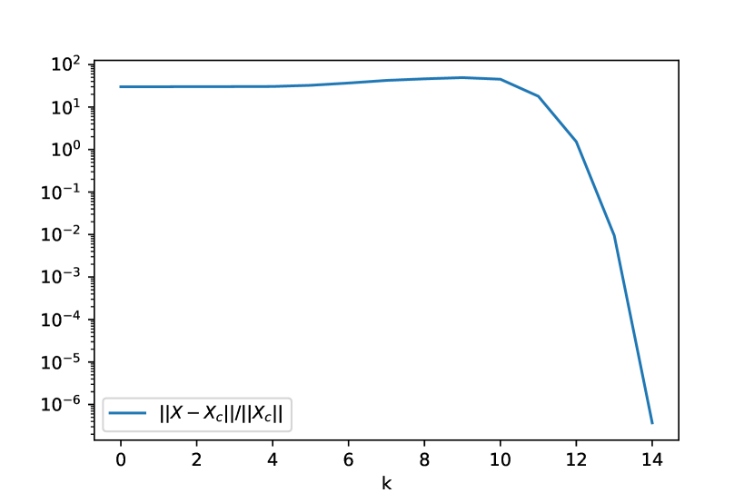
(a) Convergence of the relative error between the current solution $X_{k}$ and the analytic center $X_{c}$

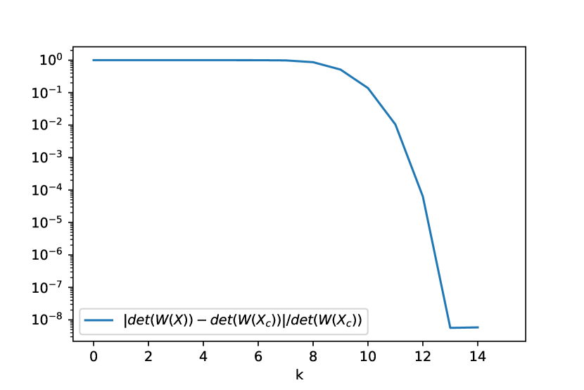
(b) Convergence of the relative error between the current value of the objective function $\det(W_{c}(X_{k}))$ and the value $\det(W_{c}(X_{c}))$ at the analytic center

Figure 1: Convergence behavior for the Newton method applied to the example as in Example 4.1

5 Computation of bounds for the passivity radius

Once we have found a solution $X\in{\mathbb{X}_{c}^{\raisebox{1.39998pt}{{$\ggcurly$}}}}$, respectively $X\in{\mathbb{X}_{d}^{\raisebox{1.39998pt}{{$\ggcurly$}}}}$, we can use this solution to find an estimate of the passivity radius of our system, i. e. the smallest perturbation $\Delta_{{\mathcal{M}}}$ to the system coefficients ${\mathcal{M}}=\{A,B,C,D\}$ that puts the system on the boundary of the set of passive systems, so that an arbitrary small further perturbation makes the system non-passive. In this section we derive lower bounds for the passivity radius in terms of the smallest eigenvalue of a scaled version of the matrices $W_{c}(X,{\mathcal{M}})$ or $W_{d}(X,{\mathcal{M}})$, respectively. Since the analytic center is central to the solution set of the LMI, we choose it for the realization of the transfer function, since then we expect to maximize a very good lower bound for the passivity radius.

5.1 The continuous-time case

As soon as we fix $X\in{\mathbb{X}_{c}^{\raisebox{1.39998pt}{{$\ggcurly$}}}}$, the matrix

$$W_{c}(X,{\mathcal{M}})=\left[\begin{array}[]{cc}-A^{\mathsf{H}}X-X\,A&C^{\mathsf{H}}-X\,B\\ C-B^{\mathsf{H}}X&D+D^{\mathsf{H}}\end{array}\right]$$ (85)

is linear as a function of the coefficients $A,B,C,D$. When perturbing the coefficients, we thus preserve strict passivity, as long as

$$W_{c}(X,{\mathcal{M}}+\Delta_{\mathcal{M}})$$ (86)

$$\qquad:=\left[\begin{array}[]{cc}-(A+\Delta_{A})^{\mathsf{H}}X-X\,(A+\Delta_{A})&(C+\Delta_{C})^{\mathsf{H}}-X(B+\Delta_{B}))\\ (C+\Delta_{C})-(B+\Delta_{B})^{\mathsf{H}}X&(D+\Delta_{D})+(D+\Delta_{D})^{\mathsf{H}}\end{array}\right]$$ (89)

$$\qquad\succ 0.$$ (90)

We thus suppose that $W_{c}(X,{{\mathcal{M}}})\succ 0$ and look for the smallest perturbation $\Delta_{{\mathcal{M}}}$ to our model ${\mathcal{M}}$ that makes $\det W_{c}(X,{\mathcal{M}}+\Delta_{{\mathcal{M}}})=0$. To measure the model perturbation, we propose to use the norm of the perturbation of the system pencil

$$\|\Delta_{\mathcal{M}}\|:=\left\|\left[\begin{array}[]{ccc}0&\Delta_{A}&\Delta_{B}\\ \Delta_{A}^{\mathsf{H}}&0&\Delta_{C}^{\mathsf{H}}\\ \Delta_{B}^{\mathsf{H}}&\Delta_{C}&\Delta_{D}+\Delta_{D}^{\mathsf{H}}\end{array}\right]\right\|_{2}\approx\left\|\left[\begin{array}[]{ccc}\Delta_{A}&\Delta_{B}\\ \Delta_{C}&\Delta_{D}\end{array}\right]\right\|_{2}.$$

We have the following lower bound in terms of the smallest eigenvalue $\lambda_{\min}$ of a scaled version of $W_{c}(X,{\mathcal{M}})$.

Lemma 5.1.

The $X$-passivity radius, defined for a given $X\in{\mathbb{X}_{c}^{\raisebox{1.39998pt}{{$\ggcurly$}}}}$ as

$$\rho_{\mathcal{M}}^{c}(X):=\inf_{\Delta_{\mathcal{M}}}\{\|\Delta_{\mathcal{M}}\||\det W_{c}(X,{\mathcal{M}}+\Delta_{\mathcal{M}})=0\},$$

satisfies

$$\lambda_{\min}(Y_{c}W_{c}(X,{\mathcal{M}})Y_{c})\leq\rho_{\mathcal{M}}^{c}(X),$$ (91)

for

$$Y_{c}:=\left[\begin{array}[]{cc}I_{n}+X^{2}&0\\ 0&I_{m}\end{array}\right]^{-\frac{1}{2}}\preceq I_{n+m}.$$

Proof.

We first note that

$$\det\left[\begin{array}[]{cccc}0&I_{n}&X&0\\ I_{n}&0&A+\Delta_{A}&B+\Delta_{B}\\ X&A^{\mathsf{H}}+\Delta_{A}^{\mathsf{H}}&0&C^{\mathsf{H}}+\Delta_{C}^{\mathsf{H}}\\ 0&B^{\mathsf{H}}+\Delta_{B}^{\mathsf{H}}&C+\Delta_{C}&R+\Delta_{R}^{\mathsf{H}}\end{array}\right]$$ (96)

$$\qquad=\det\left[\begin{array}[]{cc}0&I_{n}\\ I_{n}&0\end{array}\right]\det W_{c}(X,{\mathcal{M}}+\Delta_{\mathcal{M}}),$$ (99)

since $W_{c}(X,{\mathcal{M}}+\Delta_{\mathcal{M}})$ is just the Schur complement with respect to the leading $2n\times 2n$ matrix. Here we have set $R:=D+D^{\mathsf{H}}$ and $\Delta_{R}:=\Delta_{D}+\Delta_{D}^{\mathsf{H}}$.

If we introduce the $n\times(n+m)$ matrix $Z_{c}:=\left[\begin{array}[]{cc}-X&0\end{array}\right]$, then (99) is equivalent to

$$\left[\begin{array}[]{c}Z_{c}\\ I_{m+n}\end{array}\right]^{\mathsf{H}}\left[\begin{array}[]{ccc}0&A+\Delta_{A}&B+\Delta_{B}\\ A^{\mathsf{H}}+\Delta_{A}^{\mathsf{H}}&0&C^{\mathsf{H}}+\Delta_{C}^{\mathsf{H}}\\ B^{\mathsf{H}}+\Delta_{B}^{\mathsf{H}}&C+\Delta_{C}&R+\Delta_{R}\end{array}\right]\left[\begin{array}[]{c}Z_{c}\\ I_{m+n}\end{array}\right]=W_{c}(X,{\mathcal{M}}+\Delta_{\mathcal{M}}).$$

If we replace the matrix $\left[\begin{array}[]{c}Z_{c}\\ I_{m+n}\end{array}\right]$ by the matrix $U_{c}=\left[\begin{array}[]{c}Z_{c}\\ I_{m+n}\end{array}\right]Y_{c}$ with orthonormal columns, which we can e. g. obtain from a QR decomposition [11], then we obtain

$$U_{c}^{\mathsf{H}}\left[\begin{array}[]{ccc}0&A+\Delta_{A}&B+\Delta_{B}\\ A^{\mathsf{H}}+\Delta_{A}^{\mathsf{H}}&0&C^{\mathsf{H}}+\Delta_{C}^{\mathsf{H}}\\ B^{\mathsf{H}}+\Delta_{B}^{\mathsf{H}}&C+\Delta_{C}&R+\Delta_{R}\end{array}\right]U_{c}$$ (103)

$$\qquad=Y_{c}W_{c}(X,{\mathcal{M}}+\Delta_{\mathcal{M}})Y_{c}$$ (104)

$$\qquad=Y_{c}W_{c}(X,{\mathcal{M}})Y_{c}+U_{c}^{\mathsf{H}}\left[\begin{array}[]{ccc}0&\Delta_{A}&\Delta_{B}\\ \Delta_{A}^{\mathsf{H}}&0&\Delta_{C}^{\mathsf{H}}\\ \Delta_{B}^{\mathsf{H}}&\Delta_{C}&\Delta_{R}\end{array}\right]U_{c}.$$ (108)

Therefore, the smallest perturbation of the matrix $Y_{c}W_{c}(X,{\mathcal{M}})Y_{c}$ to make $Y_{c}W_{c}(X,{\mathcal{M}}+\Delta_{\mathcal{M}})Y_{c}$ singular must have a 2-norm which is at least as large as $\lambda_{\min}(Y_{c}W_{c}(X)Y_{c})$, and since the perturbation is a contraction of the proposed one, the lower bound in (91) follows. ∎

5.2 The discrete-time case

In the discrete-time case, for a fixed $X$ the LMI takes the form

$$W_{d}(X)=\left[\begin{array}[]{cc}-A^{\mathsf{H}}XA+X&C^{\mathsf{H}}-A^{\mathsf{H}}XB\\ C-B^{\mathsf{H}}XA&D+D^{\mathsf{H}}-B^{\mathsf{H}}XB\end{array}\right]\succeq 0,$$ (109)

and its perturbed version is

$$W_{d}(X,{\mathcal{M}}+\Delta_{\mathcal{M}})$$ (110)

$$\quad:=\left[\begin{array}[]{cc}-(A+\Delta_{A})^{\mathsf{H}}X(A+\Delta_{A})+X&(C+\Delta_{C})^{\mathsf{H}}-(A+\Delta_{A})^{\mathsf{H}}X(B+\Delta_{B})\\ C+\Delta_{C}-(B+\Delta_{B})^{\mathsf{H}}X(A+\Delta_{A})&R+\Delta_{R}-(B+\Delta_{B})^{\mathsf{H}}X(B+\Delta_{B})\end{array}\right]$$ (113)

$$\quad\succ 0,$$ (114)

where again $R:=D+D^{\mathsf{H}}$ and $\Delta_{R}:=\Delta_{D}+\Delta_{D}^{\mathsf{H}}$.

Note that, in contrast to the continuous-time case, for given $X\in{\mathbb{X}_{d}^{\raisebox{1.39998pt}{{$\ggcurly$}}}}$ , $W_{d}(X,{\mathcal{M}}+\Delta_{{\mathcal{M}}})$ is not linear in the perturbations. Nevertheless, we have an analogous bound as in Lemma 5.1 also in the discrete-time case.

Lemma 5.2.

The $X$-passivity radius, defined for a given $X\in{\mathbb{X}_{d}^{\raisebox{1.39998pt}{{$\ggcurly$}}}}$ as

$$\rho_{\mathcal{M}}^{d}(X):=\inf_{\Delta_{\mathcal{M}}}\{\|\Delta_{\mathcal{M}}\||\det W_{d}(X,{\mathcal{M}}+\Delta_{\mathcal{M}})=0\},$$

satisfies

$$\lambda_{\min}(Y_{d}\left(W_{d}(X,{\mathcal{M}})-\left[\begin{array}[]{cc}A^{\mathsf{H}}+I_{n}\\ B^{\mathsf{H}}\end{array}\right]\frac{X}{2}\left[\begin{array}[]{cc}\Delta_{A}&\Delta_{B}\end{array}\right]-\left[\begin{array}[]{c}\Delta_{A}^{\mathsf{H}}\\ \Delta_{B}^{\mathsf{H}}\end{array}\right]\frac{X}{2}\left[\begin{array}[]{cc}A+I_{n}&B\end{array}\right]\right)Y_{d})$$ (121)

$$\qquad\leq\rho^{d}_{\mathcal{M}}(X),$$ (122)

where

$$Y_{d}:=\left[\begin{array}[]{cc}I_{n+m}+Z_{d}^{\mathsf{H}}Z_{d}\end{array}\right]^{-\frac{1}{2}}\preceq I_{n+m},\ Z_{d}=-\left[\begin{array}[]{cc}\frac{X}{2}(A+\Delta_{A}-I_{n})&\frac{X}{2}(B+\Delta_{B})\end{array}\right].$$

Proof.

We first observe that

$$\det\left[\begin{array}[]{cccc}0&I_{n}&\frac{X}{2}(A+\Delta_{A}-I_{n})&\frac{X}{2}(B+\Delta_{B})\\ I_{n}&0&A+\Delta_{A}+I_{n}&B+\Delta_{B}\\ (A^{\mathsf{H}}+\Delta_{A}^{\mathsf{H}}-I_{n})\frac{X}{2}&A^{\mathsf{H}}+\Delta_{A}^{\mathsf{H}}+I_{n}&0&C^{\mathsf{H}}+\Delta_{C}^{\mathsf{H}}\\ (B^{\mathsf{H}}+\Delta_{B}^{\mathsf{H}})\frac{X}{2}&B^{\mathsf{H}}+\Delta_{B}^{\mathsf{H}}&C+\Delta_{C}&R+\Delta_{R}\end{array}\right]$$ (127)

$$\quad=\det\left[\begin{array}[]{cc}0&I_{n}\\ I_{n}&0\end{array}\right]\det W_{d}(X,{\mathcal{M}}+\Delta_{\mathcal{M}}),$$ (130)

since again $W_{d}(X,{\mathcal{M}}+\Delta_{\mathcal{M}})$ is just the Schur complement with respect to the leading $2n\times 2n$ matrix. Note that this matrix (130) is linear in the perturbation parameters, since $X$ is fixed. Using the definition of the matrix $Z_{d}$, then from (130), it follows that we can consider

$$\left[\begin{array}[]{cc}Z_{d}^{\mathsf{H}}&I_{m+n}\end{array}\right]\left[\begin{array}[]{ccc}0&A+\Delta_{A}+I_{n}&B+\Delta_{B}\\ A^{\mathsf{H}}+\Delta_{A}^{\mathsf{H}}+I_{n}&0&C^{\mathsf{H}}+\Delta_{C}^{\mathsf{H}}\\ B^{\mathsf{H}}+\Delta_{B}^{\mathsf{H}}&C+\Delta_{C}&R+\Delta_{R}\end{array}\right]\left[\begin{array}[]{c}Z_{d}\\ I_{m+n}\end{array}\right]$$ (137)

$$\qquad=W_{d}(X,{\mathcal{M}}+\Delta_{\mathcal{M}}).$$ (138)

If we replace the matrix $\left[\begin{array}[]{c}Z_{d}\\ I_{m+n}\end{array}\right]$ by the matrix with orthonormal columns $U_{d}=\left[\begin{array}[]{c}Z_{d}\\ I_{m+n}\end{array}\right]Y_{d}$, then we have

$$U_{d}^{\mathsf{H}}\left[\begin{array}[]{ccc}0&A+\Delta_{A}+I_{n}&B+\Delta_{B}\\ A^{\mathsf{H}}+\Delta_{A}^{\mathsf{H}}+I_{n}&0&C^{\mathsf{H}}+\Delta_{C}^{\mathsf{H}}\\ B^{\mathsf{H}}+\Delta_{B}^{\mathsf{H}}&C+\Delta_{C}&R+\Delta_{R}\end{array}\right]U_{d}=Y_{d}W_{d}(X,{\mathcal{M}}+\Delta_{\mathcal{M}})Y_{d}$$

from which it follows that

$$Y_{d}W_{d}(X,{\mathcal{M}}+\Delta_{\mathcal{M}})Y_{d}=U_{d}^{\mathsf{H}}\left[\begin{array}[]{ccc}0&\Delta_{A}&\Delta_{B}\\ \Delta_{A}^{\mathsf{H}}&0&\Delta_{C}^{\mathsf{H}}\\ \Delta_{B}^{\mathsf{H}}&\Delta_{C}&\Delta_{R}\end{array}\right]U_{d}$$ (142)

$$+Y_{d}\left(W_{d}(X,{\mathcal{M}})-\left[\begin{array}[]{cc}A^{\mathsf{H}}+I_{n}\\ B^{\mathsf{H}}\end{array}\right]\frac{X}{2}\left[\begin{array}[]{cc}\Delta_{A}&\Delta_{B}\end{array}\right]-\left[\begin{array}[]{c}\Delta_{A}^{\mathsf{H}}\\ \Delta_{B}^{\mathsf{H}}\end{array}\right]\frac{X}{2}\left[\begin{array}[]{cc}A+I_{n}&B\end{array}\right]\right)Y_{d},$$ (149)

and the smallest perturbation of the matrix $Y_{d}W_{d}(X,{\mathcal{M}})Y_{d}$ needed to make $Y_{d}W_{d}(X,{\mathcal{M}}+\Delta_{\mathcal{M}})Y_{d}$ singular must have a 2-norm which is at least as large as

$$\lambda_{\min}(U_{d}^{\mathsf{H}}\left[\begin{array}[]{ccc}0&A+I_{n}&B\\ A^{\mathsf{H}}+I_{n}&0&C^{\mathsf{H}}\\ B^{\mathsf{H}}&C&R\end{array}\right]U_{d})\approx\lambda_{\min}(Y_{d}W_{d}(X,{\mathcal{M}})Y_{d}).$$

Again, since the perturbation is a contraction of the proposed one, the (approximate) lower bound in (122) follows. ∎

5.3 Examples with analytic solution

In this subsection, to illustrate the results, we present simple examples of scalar transfer functions ($m=1$) of first degree ($n=1$).

Consider first an asymptotically stable continuous-time system and transfer function $T(s)=d+\frac{cb}{s-a}$ i. e. with $a<0$. Then

$$W_{c}(x)=\left[\begin{array}[]{cc}-2ax&c-bx\\ c-bx&2d\end{array}\right]$$

and its determinant is $\det(W_{c}(x))=-4adx-(c-bx)^{2}$, which is maximal at the central point $x_{a}=\frac{c}{b}-\frac{2ad}{b^{2}}$. We then get

$$W_{c}(x_{a})=\left[\begin{array}[]{cc}4d\frac{a^{2}}{b^{2}}-2c\frac{a}{b}&2d\frac{a}{b}\\ 2d\frac{a}{b}&2d\end{array}\right]=\left[\begin{array}[]{cc}1&\frac{a}{b}\\ 0&1\end{array}\right].\left[\begin{array}[]{cc}p&0\\ 0&2d\end{array}\right]\left[\begin{array}[]{cc}1&0\\ \frac{a}{b}&1\end{array}\right],$$

with $p=2d\frac{a^{2}}{b^{2}}-2c\frac{a}{b}$ which implies that $\det(W_{c}(x_{a}))=2d\cdot p$. For the transfer function to be strictly passive, it must be asymptotically stable and positive on the imaginary axis and hence also at $0$ and $\infty$. Thus, we have the conditions

$$a<0,\ d>0,\ \frac{da-cb}{a}>0.$$ (150)

The function $\Phi_{c}(\imath\omega)=2d-\frac{2acb}{a^{2}+\omega^{2}}$ is a unimodal function, which reaches its minimum either at $0$ (namely $\Phi_{c}(0)=p\frac{b^{2}}{a^{2}}$) or at $\infty$ (namely $\Phi_{c}(\infty)=2d$) and hence the conditions in (150) are sufficient to check passivity. Thus, for the model ${\mathcal{M}}$, strict passivity gets lost when either one of the following happens

$$d+\delta_{d}=0,\quad a+\delta_{a}=0,\quad\left[\begin{array}[]{cc}c+\delta_{c}&d+\delta_{d}\end{array}\right]\left[\begin{array}[]{c}-b-\delta_{b}\\ a+\delta_{a}\end{array}\right]=0.$$

Therefore, it follows that

$$\rho=\min\left(d,a,\sigma_{2}\left[\begin{array}[]{ccc}a&b\\ c&d\end{array}\right]\right)=\sigma_{2}\left[\begin{array}[]{ccc}a&b\\ c&d\end{array}\right]$$

At the analytic center $x_{a}$ we have

$$\det W_{c}(x_{a})=2dp=4\frac{ad}{b^{2}}(ad-bc)$$

and the smallest perturbation of the parameters that makes this determinant go to $0$, yields exactly the same conditions as (150). This illustrates that the $X$-passivity radius at the analytic center yields a very good condition for strict passivity of the model.

In the discrete-time case the transfer function is $T(z)=d+\frac{cb}{z-a}$ and for it be asymptotically stable we need $a^{2}<1$, when we assume the coefficients to be real. Then

$$W_{d}(x)=\begin{bmatrix}x-a^{2}x&c-abx\\ c-abx&2d-b^{2}x\end{bmatrix}$$

and the analytic center, where $\det W_{d}(x)=(1-a^{2})x(2d-b^{2}x)-(c-abx)^{2}$ is maximal, is given by $x_{a}=\frac{d-a^{2}d+abc}{b^{2}}$ with

$$\det W_{d}(x_{a})=\frac{\left(a^{2}-1\right)(bc-(a-1)d)(bc-(a+1)d)}{b^{2}}.$$

The function $\Phi_{d}(z)=\frac{bc}{\frac{1}{z}-a}+\frac{bc}{z-a}+2d$ will be minimal on the unit circle at $z=1$ or $z=-1$. Thus positivity will be lost, when either $a$ reaches $1$ or $-1$, or $bc-(a-1)d=0$ or $bc-(a+1)d=0$. This is exactly the condition also reflected in the determinant of $W(x_{c})$ at the analytic center $x_{a}$. This again illustrates that the $X$-passivity radius at the analytic center gives a good bound the passivity radius of the system.

6 Concluding remarks

We have derived conditions for the analytic center of the linear matrix inequalities (LMIs) associated with the passivity of linear continuous-time or discrete-time systems. We have presented numerical methods to compute these analytic centers with steepest ascent and Newton-like methods and we have presented lower bounds for the passivity radii associated with the LMIs evaluated at the respective analytic center.

Appendix A Derivatives of functions of complex matrices

In this appendix we present a precise derivation of the formulas for the differentiation of a matrix function with respect to a complex matrix. Here we distinguish between complex vector spaces $\mathbb{C}^{n}$ and the corresponding real vector space $\mathbb{R}^{n}+\imath\mathbb{R}^{n}$. Both spaces can be identified by $\mathbf{c}:\mathbb{C}^{n}\rightarrow\mathbb{R}^{n}+\imath\mathbb{R}^{n},\,\mathbf{c}(v)=\Re(v)+\imath\Im({v})$. For matrix spaces of dimension $m\times n$ we use the usual identification with the vector spaces $\mathbb{C}^{n}$ and $\mathbb{R}^{n}+\imath\mathbb{R}^{n}$. The space $\mathbb{C}^{n}$ is equipped with the standard scalar product $\langle x,y\rangle_{\mathbb{C}}:=x^{\mathsf{H}}y$. By $\frac{\partial}{\partial X}$ we denote the differentiation in a real vector space, whereas the differentiation of a holomorphic function $g$ is denoted by $g^{\prime}$. Note that if we write $\mathbf{c}\circ g(x)=u(x_{r}+\imath x_{i})+\imath v(x_{r}+\imath x_{i})$, then by the Cauchy-Riemann equations, see e. g. [9], we have $\mathbf{c}\circ g^{\prime}(x)=\frac{\partial}{\partial x_{r}}u(x_{r}+\imath x_{i})-\imath\frac{\partial}{\partial x_{i}}u(x_{r}+\imath x_{i}).$ Then we have the following result:

Lemma A.1.

Assume that $g:\mathbb{C}^{\IfSubStr{n}{+}{(n)}{n}\times\IfSubStr{n}{+}{(n)}{n}}\rightarrow\mathbb{C}$ is holomorphic. Then $f:\mathbb{R}^{\IfSubStr{n}{+}{(n)}{n}\times\IfSubStr{n}{+}{(n)}{n}}+\imath\mathbb{R}^{\IfSubStr{n}{+}{(n)}{n}\times\IfSubStr{n}{+}{(n)}{n}}\rightarrow\mathbb{R}$ defined by

$$f(X_{r}+\imath X_{i}):=\Re g(X)$$ (151)

is differentiable over $\mathbb{R}$ with

$$\frac{\partial}{\partial X}f(X_{r}+\imath X_{i})=\Re(\overline{g^{\prime}(X)}\circ\mathbf{c^{-1}})$$ (152)

and

$$\Big{\langle}\frac{\partial}{\partial X}f(X_{r}+\imath X_{i}),\Delta\Big{\rangle}_{\mathbb{R}}=\Re\langle\overline{g^{\prime}(X)},\mathbf{c^{-1}}(\Delta)\rangle_{\mathbb{C}},\quad\Delta=\Delta_{r}+\imath\Delta_{i}.$$ (153)

For the holomorphic function $g(X)=\det(X)$ the following fact is well-known, see e. g. [14] for a proof in the real case, that easily extends to the complex case.

Lemma A.2 (Jacobi’s formula).

Let $g(X)=\det(X)$ and $X\in\mathbb{C}^{\IfSubStr{n}{+}{(n)}{n}\times\IfSubStr{n}{+}{(n)}{n}}$. Then $g^{\prime}(X)=\operatorname{adj}(X^{T})$ and the directional derivative of $g$ in direction $\Delta\in\mathbb{C}^{\IfSubStr{n}{+}{(n)}{n}\times\IfSubStr{n}{+}{(n)}{n}}$ equals

$$g^{\prime}(X)\circ\Delta=\operatorname{tr}(\operatorname{adj}(X)\Delta)=\langle\operatorname{adj}(X)^{\mathsf{H}},\Delta\rangle_{\mathbb{C}}.$$ (154)

Applying the chain-rule we finally obtain the differentiation formula, which is used throughout this paper.

Corollary A.1.

Let $f:\mathbb{R}^{\IfSubStr{n}{+}{(n)}{n}\times\IfSubStr{n}{+}{(n)}{n}}+\imath\mathbb{R}^{\IfSubStr{n}{+}{(n)}{n}\times\IfSubStr{n}{+}{(n)}{n}}\rightarrow\mathbb{R}$ with $f(X_{r}+\imath X_{i})=\ln\Re\det(X)$ and $X\in\mathbb{C}^{\IfSubStr{n}{+}{(n)}{n}\times\IfSubStr{n}{+}{(n)}{n}}$ with $\Re\det(X)>0$. Then

$$\frac{\partial}{\partial X}f(X_{r}+\imath X_{i})=\mathbf{c}\circ\left(\frac{\overline{\det(X)}}{\Re\det(X)}X^{-\mathsf{H}}\right).$$ (155)

Appendix B Differences between continuous-time and discrete-time systems

Usually, statements for a continuous linear time-invariant system can be transformed back and forth to discrete-time systems using some bilinear transform. However, the equations determining the analytic center in both cases are cubic in $X$, which suggests that there might not be a one-to-one correspondence. We have shown that the eigenvalues of the feedback system matrix $A_{F_{c}}$ at the analytic center lie on the imaginary axis in the continuous-time case, whereas they lie inside the unit disk in the discrete-time setting. In this appendix we show that it is indeed necessary to consider the continuous-time and discrete-time case separately by showing that the three equations determining the analytic center are not preserved under the usual bilinear transformations.

B.1 Bilinear transformations

The bilinear transformation $s=(z-1)/(z+1)$ maps every asymptotically stable continuous-time system $\{A_{c},B_{c},C_{c},D_{c}\}$ to a corresponding asymptotically stable discrete-time system $\{A_{d},B_{d},C_{d},D_{d}\}$. For some $Q_{c},Q_{d}\in\mathbb{C}^{\IfSubStr{n}{+}{(n)}{n}\times\IfSubStr{n}{+}{(n)}{n}}$ and $R_{c}=D_{c}+D_{c}^{\mathsf{H}},\,R_{d}=D_{d}+D_{d}^{\mathsf{H}}$ set

$$W_{c}:=\left[\begin{array}[]{cc}Q_{c}&C_{c}^{\mathsf{H}}\\ C_{c}&R_{c}\end{array}\right],\qquad W_{d}:=\left[\begin{array}[]{cc}Q_{d}&C_{d}^{\mathsf{H}}\\ C_{d}&R_{d}\end{array}\right].$$ (156)

Then, starting from a continuous-time system $\{A_{c},B_{c},C_{c},D_{c}\}$ we obtain a transformed discrete-time system by setting

$$\begin{split}A_{d}&:=(A_{c}-I)^{-1}(I+A_{c})\\ B_{d}&:=\sqrt{2}(A_{c}-I)^{-1}B_{c}\\ T_{c}&:=\left[\begin{array}[]{cc}\sqrt{2}(I-A_{c})^{-1}&(I-A_{c})^{-1}B_{c}\\ 0&I\end{array}\right],\\ W_{d}&:=T^{\mathsf{H}}_{c}W_{c}T_{c},\end{split}$$ (157)

where $C_{d},D_{d},$ and $Q_{d}$ are obtained from $W_{d}$. Vice versa, starting from a discrete-time system $\{A_{d},B_{d},C_{d},D_{d}\}$ and using the inverse transformation $z=(1+s)/(1-s)$ we obtain a continuous-time system by setting

$$A_{c} :=(A_{d}+I)^{-1}(A_{d}-I)$$

$$B_{c} :=\sqrt{2}(A_{d}+I)^{-1}B_{d}$$

$$T_{d} :=\left[\begin{array}[]{cc}\sqrt{2}(I+A_{d})^{-1}&-(I+A_{d})^{-1}B_{d}\\ 0&I\end{array}\right],$$ (160)

$$W_{c} :=T^{\mathsf{H}}_{d}W_{d}T_{d}.$$

Note that $(I-A_{d})=2(I-A_{c})^{-1}$.

Bilinear transformations preserve asymptotic stability, and they also relate the domains of the continuous-time and discrete-time linear matrix inequalities. To see this, we express the two LMIs as

$$W_{c}(X) :=\left[\begin{array}[]{cc}Q_{c}&C_{c}^{\mathsf{H}}\\ C_{c}&R_{c}\end{array}\right]-\left[\begin{array}[]{cc}A^{\mathsf{H}}_{c}&I\\ B^{\mathsf{H}}_{c}&0\end{array}\right]\left[\begin{array}[]{cc}0&X_{c}\\ X_{c}&0\end{array}\right]\left[\begin{array}[]{cc}A_{c}&B_{c}\\ I&0\end{array}\right]\succeq 0,$$ (169)

$$W_{d}(X) :=\left[\begin{array}[]{cc}Q_{d}&C_{d}^{\mathsf{H}}\\ C_{d}&R_{d}\end{array}\right]-\left[\begin{array}[]{cc}A^{\mathsf{H}}_{d}&I\\ B^{\mathsf{H}}_{d}&0\end{array}\right]\left[\begin{array}[]{cc}X_{d}&0\\ 0&-X_{d}\end{array}\right]\left[\begin{array}[]{cc}A_{d}&B_{d}\\ I&0\end{array}\right]\succeq 0,$$ (178)

respectively. Since

$$\left[\begin{array}[]{cc}0&X_{c}\\ X_{c}&0\end{array}\right]=\left[\begin{array}[]{cc}I&I\\ I&-I\end{array}\right]\left[\begin{array}[]{cc}\frac{X_{c}}{2}&0\\ 0&-\frac{X_{c}}{2}\end{array}\right]\left[\begin{array}[]{cc}I&I\\ I&-I\end{array}\right],$$

we can also express $W_{c}(X_{c})$ as

$$W_{c}(X_{c})=\left[\begin{array}[]{cc}Q_{c}&C_{c}^{\mathsf{H}}\\ C_{c}&R_{c}\end{array}\right]-\left[\begin{array}[]{cc}A_{c}+I&B_{c}\\ A_{c}-I&B_{c}\end{array}\right]^{\mathsf{H}}\left[\begin{array}[]{cc}\frac{X_{c}}{2}&0\\ 0&-\frac{X_{c}}{2}\end{array}\right]\left[\begin{array}[]{cc}A_{c}+I&B_{c}\\ A_{c}-I&B_{c}\end{array}\right].$$

Applying the congruence transformation $T_{c}$ defined in (157), then

$$T^{\mathsf{H}}_{c}W_{c}(X_{c})T_{c}=\left[\begin{array}[]{cc}Q_{d}&C^{\mathsf{H}}_{d}\\ C_{d}&R_{d}\end{array}\right]-\left[\begin{array}[]{cc}A^{\mathsf{H}}_{d}&I\\ B^{\mathsf{H}}_{d}&0\end{array}\right]\left[\begin{array}[]{cc}X_{d}&0\\ 0&-X_{d}\end{array}\right]\left[\begin{array}[]{cc}A_{d}&B_{d}\\ I&0\end{array}\right],$$

with $A_{d},B_{d},C_{d},D_{d}$ and $Q_{d}$ defined as in (157). This shows that maximizing $\det W_{d}(X_{d})$ over $X_{d}$ and maximizing $\det W_{c}(X_{c})$ over $X_{c}$ is equivalent. Thus, the respective solutions at the continuous-time and discrete-time analytic center coincide, i. e. $X_{d}=X_{c}$. The bilinear transformation also preserves the solution of the Riccati equation as well as the domain of the linear matrix inequality. For the transformation of the matrices $C_{c}$, $D_{c}$, and $Q_{c}$ we obtain

$$\begin{bmatrix}Q_{d}&C_{d}^{\mathsf{H}}\\ C_{d}&D_{d}+D_{d}^{\mathsf{H}}\end{bmatrix}=T_{c}^{\mathsf{H}}\begin{bmatrix}Q_{c}&C_{c}^{\mathsf{H}}\\ C_{c}&D_{c}+D_{c}^{\mathsf{H}}\end{bmatrix}T_{c}=T_{c}^{\mathsf{H}}\begin{bmatrix}\sqrt{2}Q_{c}(I-A_{c})^{-1}&Q_{c}(I-A_{c})^{-1}B_{c}+C_{c}^{\mathsf{H}}\\ \sqrt{2}C_{c}(I-A_{c})^{-1}&C_{c}(I-A_{c})^{-1}B_{c}+D_{c}+D_{c}^{\mathsf{H}}\end{bmatrix}$$ (179)

where the $(1,1)$, $(1,2)$, $(2,2)$ blocks are given by

$$2(I-A_{c})^{-\mathsf{H}}Q_{c}(I-A_{c})^{-1},$$ (180)

$$\sqrt{2}(I-A_{c})^{-\mathsf{H}}Q_{c}(I-A_{c})^{-1}B_{c}+\sqrt{2}(I-A_{c})^{-\mathsf{H}}C_{c}^{\mathsf{H}},$$ (181)

$$(I-A_{c})^{-1}B_{c}+B_{c}^{\mathsf{H}}(I-A_{c})^{-\mathsf{H}}Q_{c}(I-A_{c})^{-1}B_{c}+B_{c}^{\mathsf{H}}(I-A_{c})^{-\mathsf{H}}C_{c}^{\mathsf{H}}+D_{c}+D_{c}^{\mathsf{H}},$$ (182)

respectively.

The transfer function also does not change, provided that one rephrases it in terms of the new variable, i. e. $\Phi_{d}(z)=\Phi_{c}(s)$. This can be seen as follows. Let us replace the variable $z$ of the system matrix $S_{W_{d}}(z)$ by $(1+s)/(1-s)$ and then scale the first block row and block column by $(1-s)$ and transform the second block row and block column by the upper triangular congruence transformation $T_{d}$, which does not change the transfer function, then we obtain

$$\left[\begin{array}[]{c|c}(1-s)I_{n}&0\\ \hline\cr 0&T_{d}^{\mathsf{H}}\end{array}\right] \left[\begin{array}[]{c|cc}0&A_{d}-zI_{n}&B_{d}\\ \hline\cr zA^{\mathsf{H}}_{d}-I_{n}&Q_{d}&C^{\mathsf{H}}_{d}\\ zB^{\mathsf{H}}_{d}&C_{d}&R_{d}\end{array}\right]\left[\begin{array}[]{c|c}(1-s)I_{n}&0\\ \hline\cr 0&T_{d}\end{array}\right]$$ (190)

$$\qquad=\left[\begin{array}[]{c|cc}0&A_{c}-sI_{n}&B_{c}\\ \hline\cr A^{\mathsf{H}}_{c}+sI_{n}&Q_{c}&C^{\mathsf{H}}_{c}\\ B^{\mathsf{H}}_{c}&C_{c}&R_{c}\end{array}\right].$$ (194)

B.2 Transformation of the deflating subspaces

Following [7] we consider the pencils

$$s\mathcal{E}_{c}-\mathcal{A}_{c}=\begin{bmatrix}0&-sI+A_{c}&B_{c}\\ sI+A_{c}^{\mathsf{H}}&Q_{c}&C_{c}^{\mathsf{H}}\\ B_{c}^{\mathsf{H}}&C_{c}&D_{c}+D_{c}^{\mathsf{H}}\end{bmatrix}$$ (195)

corresponding to the continuous-time case and

$$z\mathcal{A}_{d}^{\mathsf{H}}-\mathcal{A}_{d}=\begin{bmatrix}0&zI-A_{d}&-B_{d}\\ zA_{d}^{\mathsf{H}}-I&(z-1)Q_{d}&(z-1)C_{d}^{\mathsf{H}}\\ zB_{d}^{\mathsf{H}}&(z-1)C_{d}&(z-1)(D_{d}+D_{d}^{\mathsf{H}})\end{bmatrix}$$ (196)

corresponding to the discrete-time case.

If $X$ is solution of $\mathsf{Ricc}_{d}(X)=-Q_{d}$, then there is a deflating subspace of the form

$$\begin{bmatrix}0&A_{d}-zI&B_{d}\\ I-zA_{d}^{\mathsf{H}}&(z-1)Q_{d}&(z-1)C_{d}^{\mathsf{H}}\\ -zB_{d}^{\mathsf{H}}&(z-1)C_{d}&(z-1)(D_{d}+D_{d}^{\mathsf{H}})\end{bmatrix}\begin{bmatrix}-X\left(I-A_{d}+B_{d}F_{d}\right)\\ I\\ -F_{d}\end{bmatrix}$$ (197)

$$\qquad=\begin{bmatrix}I\\ (I-A_{d}^{\mathsf{H}})X\\ -B_{d}^{\mathsf{H}}X\end{bmatrix}\left(A_{d}-B_{d}F_{d}-zI\right).$$ (198)

Applying a generalized bilinear transformation to the pencil $s\mathcal{E}_{c}-\mathcal{A}_{c}$ gives

$$z\hat{\mathcal{A}}_{d}-\hat{\mathcal{A}}^{\mathsf{H}}_{d}:=z(\mathcal{E}_{c}-\mathcal{A}_{c})-(-\mathcal{E}_{c}-\mathcal{A}_{c})$$ (199)

$$\qquad=\begin{bmatrix}0&z(A_{c}-I)-(I+A_{c})&zB_{c}-B_{c}\\ -z(I+A_{c}^{\mathsf{H}})-(A_{c}^{\mathsf{H}}-I)&(z-1)Q_{c}&(z-1)C_{c}^{\mathsf{H}}\\ -zB_{c}^{\mathsf{H}}-B_{c}^{\mathsf{H}}&(z-1)C_{c}&(z-1)(D_{c}+D_{c}^{\mathsf{H}})\end{bmatrix},$$ (200)

and then performing the bilinear transform from the previous section on the last two block columns and rows, we obtain the new pencil

$$z\check{\mathcal{A}_{d}}-\check{\mathcal{A}_{d}}^{\mathsf{H}}:=\begin{bmatrix}\frac{1}{\sqrt{2}}I&0\\ 0&T_{c}^{\mathsf{H}}\end{bmatrix}\left(z\hat{\mathcal{A}_{d}}-\hat{\mathcal{A}_{d}}^{\mathsf{H}}\right)\begin{bmatrix}\frac{1}{\sqrt{2}}I&0\\ 0&T_{c}\end{bmatrix}=\begin{bmatrix}0&A_{d}-zI&B_{d}\\ I-zA_{d}^{\mathsf{H}}&(z-1)Q_{d}&(z-1)C_{d}^{\mathsf{H}}\\ -zB_{d}^{\mathsf{H}}&(z-1)C_{d}&(z-1)(D_{d}+D_{d}^{\mathsf{H}})\end{bmatrix}.$$ (201)

If, conversely, there is a continuous-time solution $X$ of $\mathsf{Ricc}_{c}(X)=-Q_{c}$, we have the deflating subspace

$$\begin{bmatrix}0&-sI+A_{c}&B_{c}\\ sI+A_{c}^{\mathsf{H}}&Q_{c}&C_{c}^{\mathsf{H}}\\ B_{c}^{\mathsf{H}}&C_{c}&D_{c}+D_{c}^{\mathsf{H}}\end{bmatrix}\begin{bmatrix}-X\\ I\\ -F_{c}\end{bmatrix}=\begin{bmatrix}I\\ X\\ 0\end{bmatrix}\left(A_{c}-B_{c}F_{c}-sI\right).$$ (202)

Then, using the same transformation we obtain

$$\left(z\check{\mathcal{A}_{d}}-\check{\mathcal{A}_{d}}^{\mathsf{H}}\right)\begin{bmatrix}\sqrt{2}I&0\\ 0&T_{c}^{-1}\end{bmatrix}\begin{bmatrix}-X\\ I\\ -F_{c}\end{bmatrix}(I-A_{c}+B_{c}F_{c})^{-1}$$ (203)

$$\qquad=\begin{bmatrix}\frac{1}{\sqrt{2}}I&0\\ 0&T_{c}^{\mathsf{H}}\end{bmatrix}\begin{bmatrix}I\\ X\\ 0\end{bmatrix}\left(z(-I+A_{c}-B_{c}F_{c})-(I+A_{c}-B_{c}F_{c})\right)(I-A_{c}+B_{c}F_{c})^{-1},$$ (204)

which is equivalent to

$$\left(z\check{\mathcal{A}_{d}}-\check{\mathcal{A}_{d}}^{\mathsf{H}}\right)\begin{bmatrix}-X(I-A_{F_{d}})\\ I\\ -\sqrt{2}F_{c}(I-A_{c}+B_{c}F_{c})^{-1}\end{bmatrix}=\begin{bmatrix}I\\ (I-A_{d})^{\mathsf{H}}X\\ -B_{d}^{\mathsf{H}}X\end{bmatrix}\left(A_{F_{d}}-zI\right),$$ (205)

where $A_{F_{d}}$ denotes the bilinear transform of the matrix $A_{F_{c}}=A_{c}-B_{c}F_{c}$. Thus, the transformed feedback matrix $F_{d}$ can be defined by

$$F_{d}:=\sqrt{2}F_{c}(I-A_{c}+B_{c}F_{c})^{-1}.$$ (206)

It needs to be analyzed how the Riccati operator $P_{c}(X)$ is transformed for a fixed $X$. Clearly, then $X$ fulfills the Riccati equation $\mathsf{Ricc}_{c}(X)=-Q_{c}$ with $Q_{c}:=-P_{c}(X)$. From the equations $\mathsf{Ricc}_{c}(X)=-Q_{c}$ and $\mathsf{Ricc}_{d}(X)=-Q_{d}$ one would then expect, that $P_{d}(X)=-Q_{d}$. However, we have the relation

$$\begin{bmatrix}P_{d}&0\\ 0&R_{d}-B_{d}^{\mathsf{H}}XB_{d}\end{bmatrix}=\left(T_{P}\right)^{\mathsf{H}}\begin{bmatrix}P_{c}&0\\ 0&R_{c}\end{bmatrix}\underbrace{\begin{bmatrix}I&0\\ F_{c}&I\end{bmatrix}\begin{bmatrix}\sqrt{2}(I-A_{c})^{-1}&(I-A_{c})^{-1}B_{c}\\ 0&I\end{bmatrix}\begin{bmatrix}I&0\\ -F_{d}&I\end{bmatrix}}_{T_{P}:=},$$ (207)

where we compute

$$T_{P}=\begin{bmatrix}\sqrt{2}(I-A_{c}+B_{c}F_{c})^{-1}&(I-A_{c})^{-1}B_{c}\\ 0&I+F_{c}(I-A_{c})^{-1}B_{c}\end{bmatrix},$$ (208)

and used that $\sqrt{2}F_{c}(I-A_{c})^{-1}-F_{d}-F_{c}(I-A_{c})^{-1}B_{c}F_{d}=0$. We thus obtain that

$$P_{d}=2(I-A_{c}+B_{c}F_{c})^{-\mathsf{H}}P_{c}(I-A_{c}+B_{c}F_{c})^{-1},$$ (209)

which, by considering that $P_{c}\succ 0$ and equation (179), only coincides with $-Q_{d}$ if $F_{c}=0$. Thus we have shown, that if we enforce a feedback, that keeps the feedback system matrix $A_{F_{d}}$ on the unit circle, then the transformed residual of the Riccati operator $P_{c}$ does not correspond to the discrete-time residual $P_{d}$. In other words, since relation (207) has to hold, the transformation of the feedback (206) cannot be true, and thus the discrete-time feedback system matrix $A_{F_{d}}$ does not lie on the unit circle. Indeed, as mentioned before, the eigenvalues lie strictly inside the unit circle.

References

• [1] D. Bankmann, V. Mehrmann, Y. Nesterov, and P. Van Dooren. Code and examples for the paper ’Computation of the analytic center of the solution set of the linear matrix inequality arising in continuous- and discrete-time passivity analysis’, April 2019. URL: https://doi.org/10.5281/zenodo.2643171, doi:10.5281/zenodo.2643171.
• [2] C. Beattie, V. Mehrmann, and P. Van Dooren. Robust port-Hamiltonian representations of passive systems. Automatica, 100:182–186, February 2019. doi:10.1016/j.automatica.2018.11.013.
• [3] R. Bellman. Introduction to Matrix Analysis, Second Edition. Classics in Applied Mathematics. Society for Industrial and Applied Mathematics, 1997. URL: https://epubs.siam.org/doi/book/10.1137/1.9781611971170, doi:10.1137/1.9781611971170.
• [4] P. Benner, P. Losse, V. Mehrmann, and M. Voigt. Numerical linear algebra methods for linear differential-algebraic equations. In A. Ilchmann and T. Reis, editors, Surveys in Differential-Algebraic Equations III, Differential-Algebaric Equations Forum, chapter 3, pages 117–175. Springer-Verlag, Cham, Switzerland, 2015.
• [5] S. Boyd, L. El Ghaoui, E. Feron, and V. Balakrishnan. Linear Matrix Inequalities in System and Control Theory. SIAM, Philadelphia, PA, 1994.
• [6] S. Boyd and L. Vandenberghe. Convex Optimization. Cambridge University Press, New York, NY, USA, 2004.
• [7] R. Byers, D. S. Mackey, V. Mehrmann, and X. Xu. Symplectic, BVD, and palindromic eigenvalue problems and their relation to discrete-time control problems. In Collection of Papers Dedicated to the 60-th Anniversary of Mihail Konstantinov, pages 81–102. Publ. House RODINA, Sofia, 2009.
• [8] G. Freiling, V. Mehrmann, and H. Xu. Existence, uniqueness and parametrization of Lagrangian invariant subspaces. SIAM J. Matrix Anal. Appl., 23:1045–1069, 2002.
• [9] E. Freitag and R. Busam. Complex Analysis. Springer, 1 edition, 2005.
• [10] Y. Genin, Y. Nesterov, and P. Van Dooren. The analytic center of LMI’s and Riccati equations. In Control Conference (ECC), 1999 European, pages 3483–3487. IEEE, 1999.
• [11] G. H. Golub and C. F. Van Loan. Matrix Computations. Johns Hopkins Univ. Press, Baltimore, 3rd edition, 1996.
• [12] V. Ionescu, C. Oara, and M. Weiss. Generalized Riccati Theory and Robust Control: A Popov Function Approach. John Wiley & Sons Ltd., Chichester, 1999.
• [13] R. Kalman. Lyapunov functions for the problem of Lur’e in automatic control. Proc. Nat. Acad. Sciences, 49:201–205, 1963.
• [14] J. R. Magnus and H. Neudecker. Matrix Differential Calculus with Applications in Statistics and Econometrics. John Wiley, second edition, 1999.
• [15] M. Moakher. A Differential Geometric Approach to the Geometric Mean of Symmetric Positive-Definite Matrices. SIAM J. Matrix Anal. Appl., 26:735–747, 2005.
• [16] Y. Nesterov. Introductory Lectures on Convex Optimization: A Basic Course. Applied Optimization. Springer US, 2013.
• [17] V. M. Popov. Hyperstability of Control Systems. Springer-Verlag New York, Inc., Secaucus, NJ, USA, 1973.
• [18] A. J. van der Schaft. Port-Hamiltonian systems: network modeling and control of nonlinear physical systems. In Advanced Dynamics and Control of Structures and Machines, CISM Courses and Lectures, Vol. 444. Springer Verlag, New York, N.Y., 2004.
• [19] A. J. van der Schaft and D. Jeltsema. Port-Hamiltonian systems theory: An introductory overview. Found. Trends Syst. Control, 1(2-3):173–378, 2014.
• [20] J. C. Willems. Least squares stationary optimal control and the algebraic Riccati equation. IEEE Trans. Automat. Control, 16(6):621–634, 1971.
• [21] J. C. Willems. Dissipative dynamical systems – Part I: General theory. Arch. Ration. Mech. Anal., 45:321–351, 1972.
• [22] J. C. Willems. Dissipative dynamical systems – Part II: Linear systems with quadratic supply rates. Arch. Ration. Mech. Anal., 45:352–393, 1972.
• [23] V. A. Yakubovich. Solution of certain matrix inequalities in the stability theory of nonlinear control systems. Dokl. Akad. Nauk. SSSR, 143:1304–1307, 1962.