secttoc3 secttoc sectlof

During the epoch of reionisation, neutral gas in the early Universe was ionized by hard ultraviolet radiation emitted by young stars in the first galaxies. To do so, ionizing ultraviolet photons must escape from the host galaxy. We present Hubble Space Telescope observations of the gravitationally lensed galaxy PSZ1-ARC G311.6602–18.4624, revealing bright, multiply-imaged ionizing photon escape from a compact star-forming region through a narrow channel in an optically thick gas. The gravitational lensing magnification shows how ionizing photons escape this galaxy, contributing to the re-ionisation of the Universe. The multiple sight lines to the source probe absorption by intergalactic neutral hydrogen on scales of no more than a few hundred, perhaps even less than ten, parsec.

Less than a billion years after the Big Bang, the Universe went through the epoch of reionization (EoR) (?), in which Lyman continuum radiation (LyC, ultraviolet light with wavelengths below 912 Ångström, capable of ionizing hydrogen) from the first galaxies ionized the previously neutral hydrogen in the intergalactic medium (IGM). To escape into the IGM, the ultraviolet photons must have avoided absorption by neutral hydrogen within the host galaxy. After the Universe became ionized and transparent to ionizing wavelengths, we expect many galaxies would still continue to emit LyC photons. However, only a few dozen such galaxies have been found, either in the local Universe (?, ?, ?, ?) or at intermediate redshifts ($1\lesssim z\lesssim 4$)  (?, ?, ?, ?, ?), leaving much of the radiation necessary to reionize the Universe unaccounted for.

Escape of LyC photons from galaxies is made possible by radiative or mechanical feedback from e.g. turbulence or young, hot stars, which can ionize most of the surrounding gas, or carve out channels through optically thick neutral gas (?, ?, ?, ?, ?). These escape scenarios can be distinguished by the spectral shape of the Lyman $\alpha$ (Ly$\alpha$) emission feature, an atomic emission line arising from the transition between the ground state and the first excited state in neutral hydrogen, at a wavelength of 1216 Å. Ly$\alpha$ scatters resonantly in the same neutral hydrogen that absorbs LyC, and the Ly$\alpha$ line shape is sensitive to its kinematics, geometry, and other properties  (?). Escape through an optically thin medium results in a double-peaked Lyman $\alpha$ profile with narrow separation between the peaks (?, ?, ?). This is what is typically observed in conjunction with confirmed LyC escape, except in a few ambiguous cases (?, ?).

In a riddled, optically thick neutral medium, both Ly$\alpha$ and LyC may escape freely through empty lines of sight, with little to no interaction with neutral hydrogen. Ly$\alpha$ then appears as a bright, narrow peak centered at the wavelength of the transition. If the neutral medium contains enough passageways of low optical depth, the majority of Lyman $\alpha$ photons will escape after scattering a small number of times, so the narrow central peak will dominate the line shape  (?). If only few, narrow channels are present, theory predicts that the probability for a given Ly$\alpha$ photon to escape in a few scattering events declines, and the probability of trapping in resonant scattering in the denser neutral medium rises  (?). This produces a characteristic, triple-peaked profile with a narrow, bright peak at line center, superimposed onto the typical broader, double-peaked line of an optically thick medium  (?, ?).

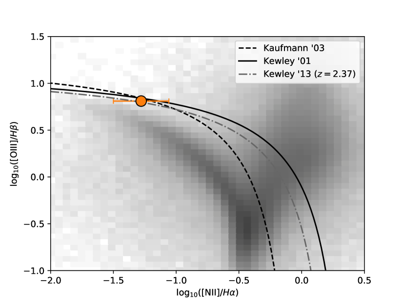
Figure S1: Baldwin, Phillips and Terlevich (BPT) diagram  (?) showing emission-line diagnostics of the Sunburst arc ionizing sources (orange point with error bars) based on Magellan/FIRE spectroscopy from previous work  (?). Overlaid are theoretical and empirical stellar/AGN separation lines  (?, ?). The grey-scale background shows a 2D histogram of 10.000 random objects from the Sloan Digital Sky Survey  (?). The grey dash-dotted curve represents a fit to the main star formation locus at $z=2.4$  (?).

Previous work has observed such a triple-peaked Lyman-$\alpha$ profile in PSZ1-ARC G311.6602–18.4624, hereafter nicknamed the Sunburst Arc  (?), a gravitationally lensed galaxy at redshift $z=2.37$ (?). The Sunburst is a single galaxy, lensed into at least 12 images by a massive foreground galaxy cluster at $z=0.44$ (?). The galaxy is young, strongly star forming, and shows no sign of an active nucleus (see fig. S1). The Lyman-$\alpha$ profile indicated that it was a prime candidate for strong LyC escape through a narrow channel oriented towards Earth (?). Such a LyC channel should appear as a multiply-imaged, compact source coincident with some of the brightest regions seen in the extended, non-ionizing stellar continuum (?) when observed using telescopes with sufficient resolution and ultraviolet capabilities.

We observed the rest-frame Lyman continuum in the Sunburst Arc using the Wide Field Camera 3 (WFC3) on the Hubble Space Telescope (HST) using the broad-band filter F275W. The wavelength cut-off of this filter matches the lowest-energy limit of the LyC at the redshift of the lensed galaxy, with only 0.5% of the total filter throughput having wavelengths longer than 912 Å. We combined the F275W observations with previous observations using the HST Advanced Camera for Surveys (ACS) and the broad-band F814W filter. At the redshift of the lensed galaxy, F814W is sensitive to non-ionizing near-UV light emitted mainly by the same young, hot stars as LyC, but is not absorbed by neutral hydrogen.

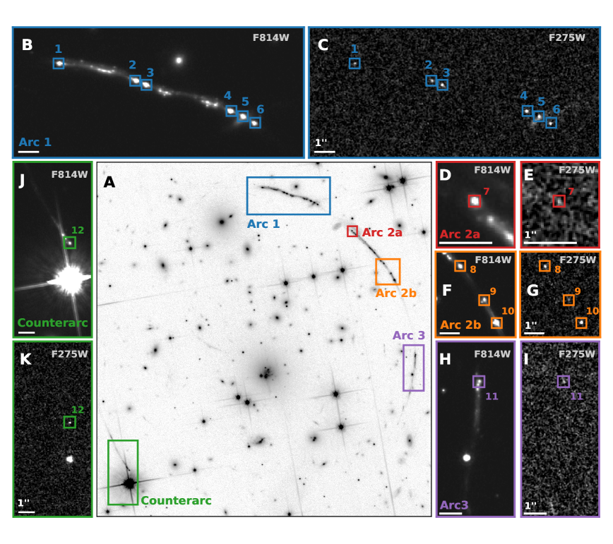
Figure 1: Comparison of ionizing and non-ionizing morphology. Panel A shows an overview of the entire arc, in the Hubble ACS F814W filter, with cutout locations marked. The surrounding panels B-K show paired F814W and F275W observations, zoomed in on the regions with confirmed Lyman Continuum detection. All panels are oriented North up and East to the left. Data in panels B-K are stretched by a hyperbolic arcsine function to balance visibility of faint features in F814W with noise in F275W panels. Panel A, in which noise is negligible, is scaled by a square root function to enhance faint features further, and colors are inverted to distinguish it from the zoomed in panels. All F814W panels except A share the same cut levels. All F275W panels share cut levels, except E and I which due to the fainter sources are cut off at 60% the upper level of the rest. The bright object near image 12 is a foreground star. 

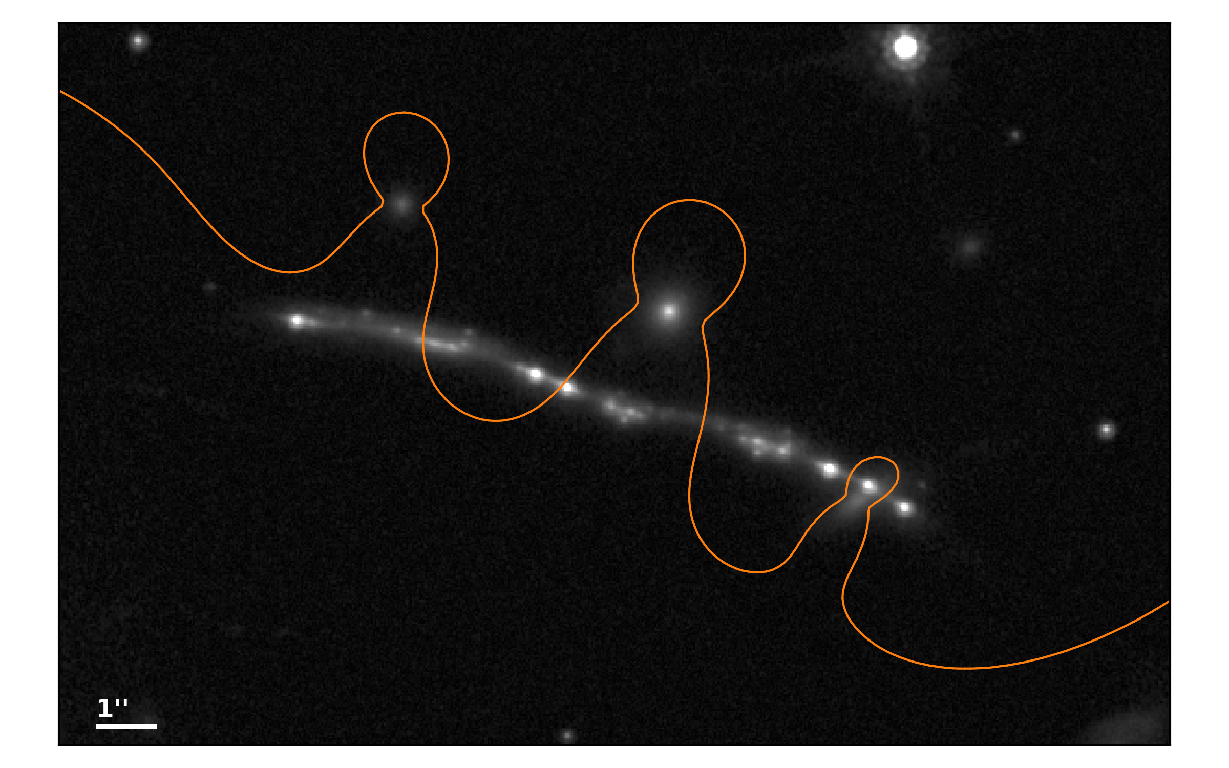
Figure S2: Critical lines in the lensing model of Arc 1. This figure shows Arc 1 as observed in F814W with the critical curve of the lens model overlaid in orange. Three members of the lensing cluster close to the line of sight produce perturbations to the large scale lensing potential which increase the image multiplicity compared to a smooth, non-perturbed potential. This arc segment contains 6 images of the leaking region (see main text). North is up, East is left. These critical curves, along with the input file used to generate them, are available as a supplementary download (Data S1)

Figure 1A shows the F814W image of the lens and arc system, while Fig. 1B-K show close-ups of regions with emission in the F275W filter. Each region is shown in both the ionizing and non-ionizing wavelengths, with the images of the LyC emitting complex marked in both filters for comparison. Image 5 is contaminated by UV continuum from a foreground galaxy which contributes $\lesssim 5\%$ to its measured flux in F814W. Lens modeling and spectroscopy show that the 12 image-plane sources of ionizing LyC emission are all lensed images of the same bright region [ (?), figure S2], with signal-to-noise ratios ranging from 4 to 42 (Table 1). The physical diameter of the LyC emitting region has an upper limit of $\sim 160$ pc (?), much smaller than the galaxy as a whole and consistent with star-forming regions in local galaxies (?).

Image	$m_{\mathrm{AB}}^{F275W}$	S/N${}_{\mathrm{\,F275W}}$	$m_{\mathrm{AB}}^{F814W}$	$f_{\mathrm{esc,rel}}\times T_{\mathrm{IGM}}$	RA,DEC (hourangle, angle)
1	26.96$\pm$0.09	$12$	22.91	23% $\pm$ 4%	15:50:07.29, -78:10:57.2
2	26.84$\pm$0.08	$13$	22.57	19% $\pm$ 3%	15:50:06.03, -78:10:58.1
3	26.18$\pm$0.05	$23$	22.68	40% $\pm$ 5%	15:50:05.86, -78:10:58.3
4	25.75$\pm$0.03	$37$	22.46	49% $\pm$ 6%	15:50:04.48, -78:10:59.6
5	26.23$\pm$0.05	$23$	23.08	55% $\pm$ 7%	15:50:04.27, -78:10:59.9
6	26.43$\pm$0.06	$19$	23.00	43% $\pm$ 6%	15:50:04.08, -78:11:00.3
7	28.24$\pm$0.30	$3.7$	23.68	14% $\pm$ 5%	15:50:02.10, -78:11:04.9
8	26.35$\pm$0.06	$19$	23.18	54% $\pm$ 7%	15:50:00.25, -78:11:10.7
9	27.34$\pm$0.15	$7.2$	23.44	27% $\pm$ 5%	15:49:59.84, -78:11:12.5
10	25.40$\pm$0.03	$42$	22.35	61% $\pm$ 8%	15:49:59.63, -78:11:13.6
11	27.58$\pm$0.18	$6.2$	23.85	32% $\pm$ 7%	15:49:58.42, -78:11:26.9
12	26.65$\pm$0.08	$15$	23.65	64% $\pm$ 9%	15:50:14.97, -78:11:47.5

Table 1: Properties of regions with detected LyC escape. The first column lists the lensed image numbers as designated in figure 1. The second and third columns show the measured apparent magnitude and signal-to-noise ratio of the LyC (F275W) observations, and the fourth column the apparent magnitudes in non-ionizing UV (F814W). The fifth column shows the apparent relative escape fractions (see main text) measured for each image. The corresponding apparent absolute escape fraction can be find by simply multiplying the relative escape fractions by a factor of $0.34\pm 0.04$, which encodes the effect of internal dust in the galaxy  (?). The sixth and last column shows the celestial right ascencion and declination in hour:minute:second, degree:minute:second. Apparent magnitudes are corrected for Milky Way dust reddening. Flux uncertainties in F814W are all $<$ 0.1%.

Measured magnitudes in both filters are tabulated in table 1, along with the computed apparent escape fraction. We computed ionizing escape fractions based on theoretical models of stellar populations  (?) which were fitted to spectroscopic observations of the non-ionizing wavelengths emitted  (?, ?) by the star forming region. From these model spectra, we predicted the intrinsic flux ratios in the F275W and F814W filters, and compared these to the observed ratios  (?). We derived both the relative and absolute escape fractions, defined as the fraction of dust-attenuated (relative) and total (absolute) ionizing radiation that escapes the neutral gas in the galaxy.

The observed flux in F275W is the radiation surviving absorption both within the source galaxy and in the IGM. Consequently, the escape fraction we derive from the flux ratios in the two filters is the combined effect of the internal and intergalactic neutral hydrogen (Hi). This quantity, found as the escape fraction from the galaxy ($f_{\mathrm{esc}}$) times the transmission coefficient of the IGM ($T_{\mathrm{IGM}}$), we refer to as the apparent escape fraction $f_{\mathrm{esc}}^{*}$. The highest measured apparent escape fraction of 64$\pm$9% (image 12) forms a lower limit to the escape fraction, corresponding to the case of a completely transparent IGM. Conversely, the apparent escape fraction in image 12 provides a lower limit to the IGM transmission of $T_{\mathrm{IGM}}\gtrsim 64\%$, as lower transmission coefficients would imply an escape fraction higher than 100%. To further constrain the line-of-sight escape fraction, we used the $T_{\textsc{igm}}$ distribution along simulated lines of sight from a previous publication  (?), and excluded the values which would lead to an escape fraction larger than 100%. From the remaining $T_{\mathrm{IGM}}$ distribution, we have extracted the 16th, 50th, and 84th percentiles and computed the corresponding escape fractions for image 12  (?). Figure 2 shows the apparent relative ($f_{\mathrm{esc,rel}}^{*}$) and absolute ($f_{\mathrm{esc,abs}}^{*}$) ionizing escape fractions along our line of sight for each lensed image, with propagated measurement uncertainties. Absolute and relative escape fractions are shown for image 12 based on the IGM transmission distribution discussed above, the 16th and 84th percentiles, and the full range bracketed by an escape fraction of 100% and the far upper end of the $T_{\mathrm{IGM}}$ distribution  (?). region coding in fig. 1. We estimate a relative line-of-sight ionizing escape fraction of $f_{\mathrm{esc,rel}}=93_{-11}^{+7}\%$, with $46\%$ as a robust lower limit (assuming a completely transparent IGM and a flux ratio $2\sigma$ below the measured value). Correcting for modeled dust absorption internal to the galaxy, we find the corresponding absolute line-of-sight escape fraction $f_{\mathrm{esc,abs}}=32^{+2}_{-4}\%$. There is however not a simple correspondence between the line-of-sight escape fraction often reported in the literature and the global ionizing escape fraction from a galaxy, unless the galaxy is perfectly isotropic. The Ly$\alpha$ profile of the Sunburst Arc  (?) indicates that its global escape fraction is much lower than the one reported here.

The computed escape fractions are subject to systematic uncertainties. The spectra used to construct the stellar populations are extracted in a larger aperture than the ones used the photometric measurements, which could affect the measured escape fractions  (?). The F814W filter, which is used to photometrically calibrate the stellar population model and predict the intrinsic LyC flux, covers an adjacent but different wavelength range than the spectra to which the stellar population model is fitted. Thus, we can not directly test the accuracy of the model in the given range when comparing it to the photometric observations. Finally, assumed stellar population models and dust attenuation laws introduce systematic uncertainties. These systematic uncertainties can affect the inferred escape fractions, but not the differences between them  (?).

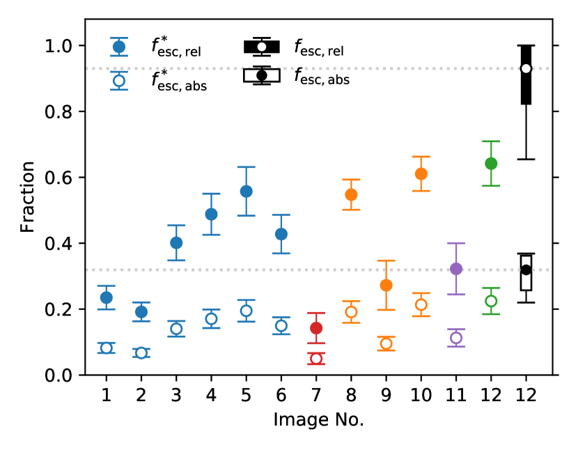
Figure 2: Lyman Continuum escape fractions. For each gravitationally lensed image, we show the fraction of the dust-attenuated (relative; filled circles) and total (absolute; empty circles) Lyman-continuum photons that reach the telescope (apparent escape fraction, $f^{*}_{\textnormal{esc}}$). Colors correspond to those in fig. 1. The black and white box-and-whiskers for image 12 show the median value (dot), 16th to 84th percentile (box) and the full allowed range (whiskers) of the relative (filled) and absolute (outlined) escape fraction corrected for modeled IGM absorption. Values are listed in Table 1.

Lensing models [see fig. S2 and  (?)] show that all ionizing sources in Arc 1, 3 and 4 (the Counterarc) are lensed images of the same system. Arc 2 has complicated lensing geometry and has not yet been possible to model completely, but from the other arc segments, we find it likely that the ionizing detections in Arc 2 are also images of the same system. This is supported by comparison of rest-frame near-UV spectra of 5 locations in Arcs 1 and 2, 4 that do and 1 that does not have detected LyC. Comparison of their stellar C iv 1550 Å and their interstellar and circumgalactic Si iv 1393,1402 Å features show that the four ionizing locations are indistinguishable, while the non-ionizing location is unambiguously different. [ (?) and fig. S2].

The lensing models indicate that the magnification factor in Arc 1 is between 10 and 30 for each image. The central Lyman-continuum source is unresolved in all images, which places an upper limit on the source size at the instrument point spread function (PSF) of $0.09^{\prime\prime}$, corresponding to around 500 pc in the lens plane. For a magnification of 10 (in area), this corresponds to a physical diameter of $\sim 160$ parsec in the source plane. With a magnification of 30, the maximum diameter would be $\sim 90$ pc, consistent with star forming regions in local galaxies (?) and at higher redshifts (?, ?).

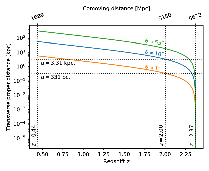
Figure 3: Transverse physical distances between lines of sight. Transverse physical separation $d$ of lines of sight with angular separations $\theta$ of 1, 10 and 55^′′ (corresponding to the distances between images 2–3, 1–6, and 6–12, respectively) in the lensing plane are shown as a function of redshift. The redshifts of the lensing plane ($z=0.44$), the lensed galaxy ($z=2.37$), and the minimum redshift of intervening H i absorption ($z\lesssim 2.0$) are marked, along with the maximum transverse distances at the point of H i absorption.

Light from the multiple lens-plane images of the source galaxy traverses different paths between their point of origin and Earth. We interpret the variations in $f^{*}_{\textnormal{esc}}$ as being due to varying amounts of absorbing neutral Hyrdogen being present along these paths. Furthermore, the absorption most likely occurs at $z\gtrsim 2$, at which redshift half of the LyC emission detected in the F275W image has been redshifted beyond the ionization limit of hydrogen  (?). In fig. 3, we show the transverse distance between lines of sight towards images 2 and 3 (one of the closest pairs), 1 and 6 (typical size of an arc segment), and 1 and 12 (on opposite sides of the arc) as a function of redshift, and mark the transverse distance between the lines of sight towards images 2 and 3 at $z=2$. At this redshift, the physical transverse distance between the lines of sight to images and 3 is $d\approx 330$ parsec.

The upper limit on the redshift of absorption depends on the combined extent of the ionizing source(s). For diameters of 160 or 30 parsec, the absorption must occur at redshifts of $z\lesssim 2.27$ or $z\lesssim 2.35$, respectively. Even for a very compact cluster a few parsecs across, the absorption must still be $\gtrsim 1$ megaparsec (Mpc) outside the galaxy. Possible absorbers include an undetected, interloping galaxy, or circumgalactic or intergalactic systems of neutral hydrogen. It is also possible that the LyC originates in just one or a few very massive O-type or Wolf-Rayet stars  (?), in which case the absorption could occur in the interstellar or circumgalactic medium (ISM or CGM, respectively) of the source galaxy itself, and the transverse separation of sight lines could be a fraction of a parsec.

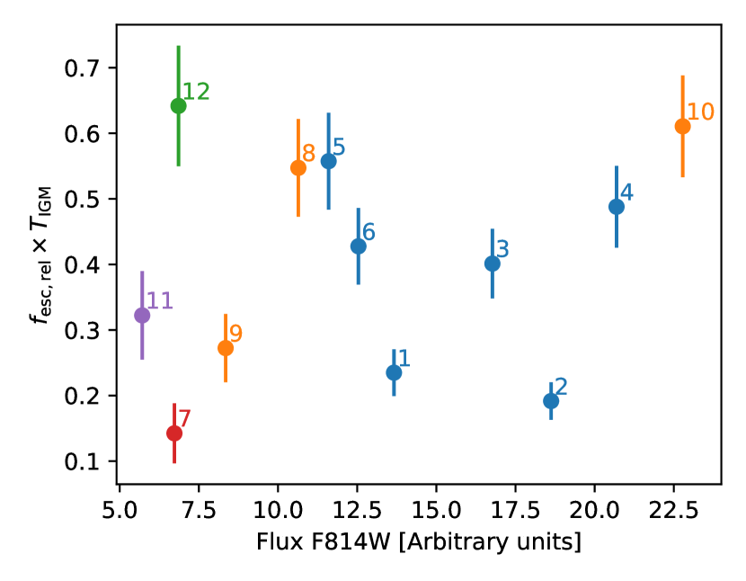
Figure S5: Flux in F814W vs. apparent escape fraction. $F_{\mathrm{814}}$ vs. apparent escape fraction is shown for each of the 12 images, with colors following the scheme established in figure 1 and  2

We considered differential magnification as a possible alternative explanation of the differences in apparent escape fraction. However, this effect would lead to a correlation between observed F814W magnitudes and $f^{*}_{\textnormal{esc}}$. With a Pearson’s $r=0.2$ and a significance of $p=0.53$, we do not find such a correlation [Fig S5,  (?)].

Supplementary materials

• Materials and Methods

• Supplementary Text

• Supplementary figures S1–S5

• References (28–55)

Acknowledgements

E.R-T thanks Stockholm University for their kind hospitality, Matthew Hayes and Angela Adamo for informative and helpful conversations, and Kaveh Vasei and coauthors for generously sharing his intermediate science products.

Funding

E.R-T and H.D. acknowledge support from the Research Council of Norway. M.G. was supported by by NASA through the NASA Hubble Fellowship grant #HST–HF2–51409 awarded by the Space Telescope Science Institute, which is operated by the Association of Universities for Research in Astronomy, Inc., for NASA, under contract NAS5–26555.

Author contributions

E.R-T. led the project and paper writing, taking input and feedback from all co-authors, especially H.D. and M.G. E.R-T. made all figures. H.D. wrote the HST proposals leading to the F275W and F814W observations, assisted by E.R-T. M.K.F. reduced and combined the images in both filters. E.R-T. performed photometry and computed escape fractions. J.C. performed stellar population synthesis based on spectroscopic observations made by J.R. and M.B and reduced by J.R. M.D.G. constructed the spatial model of flux in the MagE aperture. K.S. and G.M. produced the lens model.

Competing interests

The authors declare no competing interests.

Data and materials availability

• Raw Hubble Space Telescope WFC3 F275W and ACS F814W observations are available at the Mikulski Archive for Space Telescopes (MAST, http://archive.stsci.edu/hst/), program IDs 15418 (F275W) and 15101 (F814W).

• Raw Magellan/MagE observations and corresponding calibration data are available for download at Figshare  (?)

• Parameter file to generate our lens model with Lenstool  (?), along with a DS9 region file showing the critical curves of this model, is available for download as online supplementary materials (Data S1).

• Scripts used to generate stellar population models are available for download at Zenodo  (?).

Supplementary Materials for
Gravitational lensing reveals ionizing ultraviolet photons escaping from a distant galaxy
T. Emil Rivera-Thorsen^1∗, Håkon Dahle¹, John Chisholm^2,3,

Michael K. Florian⁴, Max Gronke⁵, Jane R. Rigby ⁴, Michael D. Gladders^6,7,

Guillaume Mahler⁸, Keren Sharon⁸, Matthew Bayliss^9,10

¹Institute of Theoretical Astrophysics, University of Oslo, Postboks 1029,0315 Oslo, Norway
²Observatoire de Genève, Université de Genève, 51 Ch. des Maillettes, 1290 Versoix, Switzerland
³Department of Astronomy and Astrophysics, University of California, Santa Cruz, CA 95064
⁴Observational Cosmology Lab, NASA Goddard Space Flight Center,
8800 Greenbelt Rd., Greenbelt, MD 20771, USA
⁵Department of Physics, University of California, Santa Barbara, CA 93106, USA
⁶Department of Astronomy and Astrophysics, University of Chicago, Chicago, IL 60637, USA
⁷Kavli Institute for Cosmological Physics, University of Chicago, Chicago, IL 60637, USA
⁸Department of Astronomy, University of Michigan,
1085 South University Avenue, Ann Arbor, MI 48109, USA
⁹Massachusetts Institute of Technology-Kavli Center for Astrophysics and Space Research,
77 Massachusetts Avenue, Cambridge, MA, 02139, USA
¹⁰Department of Physics, University of Cincinnati, Cincinnati, OH 45221, USA
^∗Correspondence to: trive@astro.su.se

This PDF file includes:

• Materials and Methods

• Supplementary Text

• Figures S1–S6

• References 28–56

Appendix A Supplementary materials

Materials and Methods

Conventions

We have assumed a flat $\Lambda$-Cold Dark Matter cosmology with Hubble expansion parameter $H_{0}=70$ km s^-1 Mpc^-1 and a matter density parameter $\Omega_{M,0}=0.3$. Flux densities are given with respect to wavelength ($f_{\lambda}$), and magnitudes are given in the $AB$ system. Celestial coordinates are given in the ICRS system. The galaxy is designated PSZ1-ARC G311.6602–18.4624 as in the discovery paper  (?). The arc segments referred to in the discovery paper  (?) as S1, S2 and S3 are here referred to as Arc 1, Arc 2 and Arc 3, respectively. The counterarc was not yet confirmed as part of the lensed system in the discovery paper.

Hubble Space Telescope observations and data reduction

The arc was observed in the UVIS channel of HST WFC3  (?) and HST ACS  (?) using the filters F275W (program ID 15418, PI: H. Dahle), and F814W (program ID 15101, PI: H. Dahle). The F275W observations, which capture Lyman continuum emission at the redshift of the arc, were carried out during two visits, one on 2018 April 8, and one on 2018 April 14 Universal Time (UT). The cumulative exposure time in the F275W filter was 9422 s. In the F814W filter, eight exposures were taken for a total of 5280 s. between UT 2018 February 21 and UT 2018 February 22. All observations were conducted using a 4-point dither pattern to minimize the effects of bad pixels and to better sample the point spread function, improving the effective resolution of the final data products. The images in each filter were aligned using the drizzlepac (?) routine tweakreg, and drizzled to a common grid with a pixel size of $0.03^{\prime\prime}$ with astrodrizzle using a Gaussian kernel and a “drop size” (final_pixfrac) of 0.8.

MagE observations and data reduction

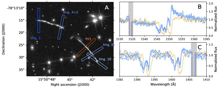
Figure S3: Spectroscopic comparison of leaking regions and non-leaking region. Panel A shows the HST ACS/F814W image zoomed in on the Arc1 and Arc2, containing images 1–10 of the LyC-leaking ionizing region, with locations of the MagE slits overlaid. Slits covering ionizing detections are blue and fully drawn, while the slit with no ionizing radiation detected is shown with orange dashes. The blue slits are named by the convention introduced in fig. 1. Panel B shows the median-normalized MagE spectra zoomed in on a narrow wavelength region containing the the C iv 1550 Å stellar wind feature, and panel C the ISM/CGM Siiv 1393,1402 Å doublet. Spectra in panels B–C are colored and shown in line style corresponding to slit color and line style in panel A, and grey shading indicates data masked out due to detector gaps.

Spectra with the Magellan Echellette spectrograph [MagE,  (?)] on the Magellan Baade telescope were obtained from four observing runs in May 2017, July 2017, April 2018, and August 2018, that covered 5 distinct image plane regions in arc segments 1 and 2, see fig. S3 for slit positions. Each region was observed with a total integration time of 2–4 hours. The $1^{\prime\prime}$ slit was used for the first two runs, and the $0.85^{\prime\prime}$ slit was used for the latter two runs, producing effective spectral resolving powers of $R\approx 4500$ and $R\approx 5200$, respectively, as measured from night sky lines. The MagE data were reduced as described in  (?), including flat-fielding, wavelength calibration, sky subtraction, extraction, flux calibration, telluric correction, and removal of Milky Way reddening. The results are one-dimensional flux- and wavelength-calibrated spectra covering 3200–8280 Å.

Photometry

We performed photometry using the source detection and photometry software Source Extractor (?) running in dual mode using the F275W observations as the detection image. The detection frames were smoothed by a narrow kernel 1.5 pixels wide to avoid spurious detections due to single noisy pixels, but fluxes were measured in the raw science frames in both filters. We extracted the fluxes in a fixed aperture 4 pixels wide at the positions of the 12 images in both of the filters.

Photometric uncertainties are dominated by the F275W observations. In F814W, the signal-to-noise ratio is $>1000$ in all photometric apertures. To measure the uncertainties in F275W, we placed 300 apertures at random positions containing only background near the source, and computed the standard deviation of these measurements. These were adopted as the standard errors for a given aperture, and propagated forward in our analysis. In a few cases, apertures placed on nearby stars had to be rejected, as they artificially inflated the standard deviations strongly.

The aperture size was selected to to optimize the balance between maximizing signal-to-noise and robustness to aperture placement (which both favor larger apertures), and minimizing contamination by the surrounding stellar population which is detected in F814W only (favors smaller apertures). While the Lyman continuum emitting cluster complex is unresolved or barely resolved in the HST observations, the observations in F814W show a complex morphology of clusters and underlying, diffuse stellar population. Thus, the measured F275W/F814W colors will depend on the chosen aperture size: larger apertures will include only the faint wings of the point spread function for the point source images in F275W, while they will include a growing contribution from the non-leaking stellar population in F814W. To determine the most appropriate aperture size, we extracted fluxes and computed flux ratios for apertures sized 2, 4, 7, and 11 pixels, corresponding to approximately 1/2, 1, 2, 3, and 4 times the full width at half maximum (FWHM) of the corrected PSF. We found that for apertures sizes $s\leq 4$ pixels, there were little difference between the measured flux ratios, reflecting that the flux inside this aperture is dominated by the leaking point sources. We thus opted for the 4 pixel aperture, to get the best possible balance between larger aperture and uncontaminated flux from the central region. We applied aperture loss corrections by dividing by encircled energy fractions of 0.598 (F275W) and 0.611 (F814W) as prescribed in the data analysis instructions from Space Telescope Science Institute  (?, ?), then computed AB magnitudes using zero points from the same publications.

Lensing model and identification of multiple images

We produced a gravitational lensing model of the source-lens system using the software package lenstool  (?). Our lensing models of the lens-source system establish that the detected occurrences of ionizing radiation in arc segments 1, 3 and 4 (Counterarc) are one source, multiply imaged by the lensing potential. In fig. S2, we show our lensing model of Arc 1. Three foreground galaxies close to the line of sight of this arc produce local perturbations to the global lensing potential, increasing the image multiplicity compared to the case of a cluster lens without any such substructure. Boundaries between separate (partial) images of the source galaxy are marked by the critical lines where they cross the arc; we find 6 separate images of the Lyman continuum emitting clump in this arc segment.

For arc segment 2, there are several plausible models that are all consistent with the data, and which do not constrain the location of the critical curves well. However, given the presence of only one LyC-emitting source in the other arc segments, we find it most likely that the detections in this arc segment are multiple images of the same image, too.

This is supported by the MagE spectra described above. Two of the spectroscopic observations covered two of the images in Arc 2, with a third covering a non-ionizing region in Arc 2 for comparison. In panels B–C in figure S3, we show plots of the spectra from the pointings shown in figure S3A, zoomed in on the stellar C iv 1550 Å and the Si iv 1393,1402 Å interstellar and circumgalactic gas lines. The former is sensitive to age and individual characteristics of a stellar population, the latter is sensitive to kinematics and ionization of the surrounding gas. The spectra have been normalized by division by their median value and smoothed by a 3 pixel boxcar kernel to reduce random noise, but have not otherwise been manipulated. The spectra from pointings with LyC detections are nearly identical in both the stellar and the ISM line, while the non-detection pointing is different in both. The spectra confirm the conclusion that the LyC leaking regions are indeed multiple images of the same region, derived independently from the lensing models discussed above.

Stellar population synthesis

The young, massive stars which produce Lyman continuum, have characteristic spectral features in the rest-frame far-ultraviolet such as broad N V 1240 Å and C IV 1550 Å stellar wind profiles  (?), and weak photospheric absorption lines  (?). These features constrain the age and metallicity of the stellar population, and, consequently, the intrinsic ionizing continuum.

We constrained the ionizing continuum by fitting the observed, Milky Way extinction-corrected MagE spectrum  (?) with fully theoretical stellar population models, following an established methodology  (?). We used the spectral region between 1240–1900 Å in the rest frame while masking regions of strong ISM absorption and emission lines as well as absorption from intervening systems. We then assumed that the far ultraviolet continuum is a discrete sum of multiple single-aged populations of O- and B-type stars. Thus, we created a linear combination of theoretical stellar templates, with ages varying between 1–40 Myr. Due to line-blanketing in the atmospheres of massive stars, the stellar metallicity also sensitively determines the ionizing continuum and we included stellar templates with metallicities of 0.05, 0.2, 0.4, 1.0, and 2.0 times the Solar metallicity Z_⊙ to account for a wide range of possible metallicities. The final suite of models consisted of 50 stellar templates (five metallicities each with 10 possible ages) and we fit for a linear coefficient multiplied to each individual theoretical stellar template using the IDL routine mpfit (?). The resulting linear combination of stellar models was attenuated by a dust attenuation law appropriate for a $z\sim 3$ starburst galaxy  (?). The attenuation parameter was left as a free parameter in our fits to find the value that best matched the observed continuum slope. We found a best-fit extinction of $E(B-V)=0.146\pm 0.003$ mag., which yields a light- and throughput-weighted attenuation in the two filters of $A_{\mathrm{F275W}}=2.06\pm 0.11$, $A_{\mathrm{F814W}}=0.92\pm 0.03$.

We used the fully theoretical, high-resolution Starburst99 stellar continuum models, compiled using the WM-Basic method  (?) with the Geneva atmospheric models with high-mass loss  (?). We assumed a Kroupa initial mass function (IMF), with a power-law index of 1.3 (2.3) for the low (high) mass slope, and a high-mass cut-off at 100 M_⊙. The fitted stellar population is dominated by a very young (a light-weighted age of 2.9 Myr), moderately metal-rich (0.56 Z_⊙) stellar population. We tested whether the assumed Starburst99 theoretical stellar templates impacted the modeled ionizing continuum by fitting the observations with bpass  (?) models, which produced similar ages, metallicities, and ionizing continua, largely because the two libraries have similar O-type stellar models (?).

The high-resolution Starburst99 models used for the fitting accurately reproduce the narrow observed spectral features, but do not extend blueward of 900 Å into the Lyman continuum  (?). Using the linear coefficients obtained from the high-resolution models, we created a low-resolution Starburst99 model, with and without attenuation. The extinction-free template models the intrinsic ionizing continuum and allows us to compare the modeled and observed Lyman continuum.

To investigate systematic uncertainties introduced by the choice of stellar population and dust models, we also created a stellar population model based on the bpass library  (?) in the same way, and performed the same fits assuming an SMC-like dust attenuation law  (?). These are compared in the Supplementary text below.

Milky Way dust correction

All measured fluxes from HST and MagE have been corrected for foreground Milky Way dust using a reddening $E(B-V)=0.09427$ mag  (?), and assuming a standard extinction law with a standard $R_{V}=3.1$ (?). The effective wavelength for each of the HST filters was determined as the average wavelength in each filter, weighted by the products of the uncorrected Starburst99 model spectrum described above, and the instrument throughput. This procedure yields multiplicative dust correction coefficients of 1.71 for F275W and 1.18 for F814W.

Emission line diagnostics

To test for signs of AGN activity, we performed the line ratio based Baldwin, Phillips, and Terlevich [BPT,  (?)] diagnostic based on a rest-frame optical Magellan/FIRE spectrum published in a previous work  (?), and compared it to theoretical and empirical distinction criteria  (?, ?) and a theoretical star formation locus accounting for the harder UV field at $z\sim 2.4$  (?). The result is shown in figure S1. We find no sign of AGN activity in the Sunburst Arc.

Supplementary text

Ionizing escape fractions

The relative and absolute LyC escape fraction are defined as the fractions of intrinsic photons that escape the gas (and dust) of the source galaxy and reaches the IGM. We have computed this based on the synthetic dust-absorbed and intrinsic spectra resulting from the stellar population modelling described above. Focusing on the relative escape fraction, it is defined as:

$$f_{\mathrm{esc,rel}}=\frac{F_{\mathrm{275}}^{\mathrm{obs}}}{F_{275}^{\mathrm{int,ext}}}\frac{1}{T_{\mathrm{IGM}}},$$ (S1)

where the numerator in the first fraction is the observed flux in the F275W filter, and the denominator is the same as we would see it through a completely ionized (but not dust-free) medium, and the transmission coefficient $T_{\mathrm{IGM}}$ is the fraction of escaping LyC that passes through the IGM without absorption. We do not know $F_{\mathrm{275}}^{\mathrm{int,ext}}$ directly, but since the non-ionizing continuum in F814W is unaffected by neutral hydrogen, we can use the theoretical spectra to compute an expected flux in F275W assuming complete transparency to LyC:

$$F_{\mathrm{275}}^{\mathrm{int,ext}}=\int L_{\mathrm{S99}}T_{\mathrm{275}}d\lambda\frac{F_{\mathrm{814}}^{\mathrm{obs}}}{\int L_{\mathrm{S99}}T_{\mathrm{814}}d\lambda}\frac{\int T_{\mathrm{814}}d\lambda}{\int T_{\mathrm{275}}d\lambda},$$ (S2)

where $F_{\mathrm{814}}^{\mathrm{obs}}$ is the observed flux in F814W, $L_{\mathrm{S99}}(\lambda)$ is the theoretical spectral flux density from Starburst99, and $T_{i}(\lambda)$ is the system transmission curves for filter $i$. Combining this with eq. S1 and rearranging, we find:

$$f_{\mathrm{esc,rel}}T_{\mathrm{IGM}}=\frac{F_{\mathrm{275}}}{F_{\mathrm{814}}}\frac{\int T_{\mathrm{275}}d\lambda}{\int T_{\mathrm{814}}d\lambda}\frac{\int L_{\mathrm{S99}}T_{\mathrm{814}}d\lambda}{\int L_{\mathrm{S99}}T_{\mathrm{275}}d\lambda}.$$ (S3)

We find the apparent absolute escape fraction by the same procedure for the unattenuated theoretical spectra from Starburst99; this yields a multiplicative factor

The escape fractions found this way are what we call the “apparent escape fractions”, as they do not account for absorption in the intergalactic medium. These are shown in figure 2 for each lensed image.

Transmission in the intergalactic medium

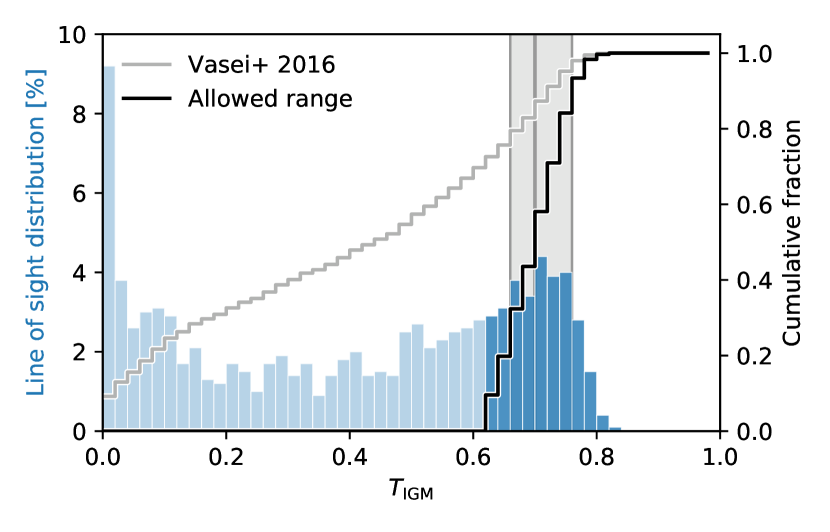
Figure S4: Simulated distribution of IGM transmission coefficients at $z=2.38$. IGM transmission histogram by Vasei et al. (?). Values excluded because they lead to escape fractions above unity are shown in lighter shade. Grey steps show the original, and black steps the updated cumulated distribution derived from the remaining, permitted values of $T_{\mathrm{IGM}}$. The 16th, 50th and 84th percentile of the updated distribution are shown as vertical grey lines with the region spanned by them shaded.

To estimate the IGM transmission, we have adopted an IGM transmission distribution  (?), which measures the IGM transmission out to $z=2.38$ along simulated lines of sight. This redshift is nearly identical to that of the Sunburst Arc, so we adopt their coefficients without modifications. The median coefficient $T_{\mathrm{IGM}}=0.4$ from that study yields a relative escape fraction for the Sunburst Arc of more than 120%. All coefficients $T_{\mathrm{IGM}}\lesssim 0.48$ are excluded in our case, because they would yield escape fractions larger than 100%. With these values excluded, we renormalized the remaining distribution and computed the cumulative probability and found the median value with 16 and 84% confidence levels. The original and updated IGM transmission histograms, with cumulated fractions, are shown in fig. S4. The modified distribution yielded a median value with 16th and 84th percentile confidence levels of $T_{\mathrm{IGM}}=0.69^{+0.06}_{-0.04}$. For the measured apparent escape fraction of image 12, this yields a relative escape fraction of $f_{\mathrm{esc,rel}}=0.93^{+0.07}_{-0.11}$ and an absolute escape fraction of $f_{\mathrm{esc,abs}}=0.32^{+0.04}_{-0.06}$. We estimated the by approximating the $T_{\mathrm{IGM}}$ distribution by an asymmetric Gaussian distribution, interpreting the 16th and 84th percentiles as standard deviations, and square-summing with the standard errors of the $f^{*}_{\mathrm{esc}}$ above.

Transverse scale of IGM probed by sight lines to multiple images

To calculate the transverse distances between sight lines, we used the approximation of a spherically symmetric lensing system with the telescope aligned with the source and the center of the lens. The ratio between transverse distances in the lens plane and in any plane between the source and the lens is then:

$$\frac{d_{i}}{d_{L}}=\frac{\left[1-\frac{D_{Li}D_{s}}{D_{Ls}D_{i}}\right]D_{i}}{D_{L}},$$ (S4)

where $d$ is the transverse physical distance, $D=D(z)$ is the cosmological angular diameter distance as a function of redshift, and the subscripts $s$, $L$ and $i$ denote source, lens, and intervening plane. In fig.3, we plot the transverse, physical distances corresponding to $1^{\prime\prime},10^{\prime\prime}\textrm{ and }55^{\prime\prime}$ in the lens plane, as function of redshift and co-moving distance. These angles are the approximate distances between images 2 and 3, across Arc 1 between images 1 and 6, and across the entire arc between images 1 and 12.

Because we found no significant contribution from differential magnification to the differences in apparent escape fraction between images in the arc, we conclude that they arise from changing column densities of neutral hydrogen along the lines of sight. Photons of wavelength longer than the Lyman $\alpha$ line at $\lambda=1216$ Å are unaffected by neutral hydrogen, so absorption variations must occur before cosmic expansion has redshifted all the intrinsically ionizing photons beyond this wavelength. In addition, it is unlikely that the variations occur due to Lyman $\alpha$ absorption in the IGM: Spectral Lyman $\alpha$ absorption features are typically narrow and strongly saturated, and a change in column density of a factor of a few will have only a small effect on the total absorbed flux. A difference of a factor 2 in transmitted flux due to varying Ly$\alpha$ absorption would require a doubling in the number of absorbing systems. In contrast, when the photons are still within the ionizing wavelength range, the transmission depends directly on the logarithm of the total column density integrated over the relevant wavelength range, and the same variation in absorption would only require a modest change in integrated Hi column density. This leads us to conclude that the absorption most likely happens when the light still has ionizing wavelengths.

As the lower redshift limit, we have adopted a redshift of absorption of $z_{\mathrm{abs}}\gtrsim 2.0$, at which half of the flux observed in F275W has redshifted out of the ionizing range. Because we have found variations in the apparent escape fraction of almost a factor of 5, this is a conservative estimate. At this redshift, the transverse distance between the lines of sight towards images 2 and 3 is determined by eqn. S4 to be $d_{23}=331$ pc. The upper redshift limit depends strongly on the physical scale of the region emitting ionizing photons. In the upper limit, the effective diameter of the knot is $\sim 160$ pc. In order to produce a difference in $f^{*}_{\textnormal{esc}}$ of a factor 2, as was the adopted requirement above, this means the transverse distance must be at least half the effective diameter, or around 80 pc. which, using eqn. S4, yields $z_{\textnormal{abs}}\lesssim 2.27$. However, the cluster may be considerably smaller than this; studies of the local Universe have found massive, luminous starburst regions as small as $\sim 5$ pc. (?), and the ionizing emission may originate from an even more compact stellar association. If this is the case, the absorption could take place in the circumgalactic medium (CGM) of the galaxy. In the extreme limit, all the ionizing radiation may originate from one or two extremely young, bright, massive stars, in which case the absorption could in principle take place in the interstellar medium of the galaxy itself, on scales of less than a parsec.

We speculate that the most likely interpretation of these variations is that they probe variation on the scale of a few tens or hundreds of parsec, either in a Lyman-limit system withing $\sim 500$ Mpc. from the galaxy, or on a scale of $\lesssim 1$ parsec in the galaxy’s own CGM.

Differential magnification

One possible explanation for the variation in the F275W/F814W flux ratios between the lensed images of the leaking region is differential magnification: If the sources of emission in F275W and F814W are not completely coincident (if e.g. the ionizing radiation is dominated by one massive Wolf-Rayet star displaced from the central stellar component), the sources and the lens caustics might be arranged in such a way as to magnify one component stronger than the other. However, this is mainly a concern when the caustics are actually crossing, or very close to, the bright sources, which makes it unlikely that this effect dominates the variations we observe. The distance between the components, if any, is unresolved in our observations and thus known to be much smaller than the distance from either to the critical lines. Still, to test this further, we consider the following:

Because the caustics do not cross the emitting region, differential magnification may only occur if one component is closer to the caustics than the other. If the center of flux in F814W is closer to the caustic than that of F275W, the stronger magnification of the non-ionizing flux will yield a lower apparent escape fraction, and vice versa.

This effect is somewhat counteracted by the presence of an extended stellar component surrounding the central, unresolved peak in F814W. In the case where the F275W source is more strongly magnified, a larger contribution from this extended component will be present in the aperture in F814W, but absent in F275W, and vice versa. This will counteract the effect described above. However, since gravitational lensing preserves surface brightness, the contribution from the extended component will change more slowly than the main source. Thus, despite the presence of this effect, we still expect to see a strong correlation between the measured F814W flux (which is unaffected by neutral hydrogen absorption) and derived apparent escape fraction, if the effect is due to differential magnification.

In fig. S5, we show a plot of the F814W fluxes vs. the apparent escape fractions. We find no significant correlation, with a measured Pearson’s $r=0.2$ and a p-value of $p=0.53$, leading us to conclude that this effect is not what causes the found variations.

Systematic uncertainties

Non-ionizing contamination in F275W
A small, but non-negligible amount of the light in F275W is transmitted redward of the observed wavelength of the Lyman edge. To ensure we are not just observing non-ionizing continuum, we have computed the expected flux in the filter by multiplying the synthetic Starburst99 spectrum by the transmission curve of F275W and integrating this on the red side of the Lyman edge only. The derived fluxes, which span from $\sim 2\%$ to $\sim 10\%$ of the measured fluxes, were then subtracted from the measured F275W fluxes to correct for the contamination. All properties derived from measured F275W are corrected for this effect.

Photometric aperture does not match spectroscopic slit
The spectroscopic slit, on which our stellar population modeling is based, is considerably larger than the photometric apertures. The line-of-sight ionizing escape fraction reported in this work is based on the assumption that the UV spectroscopic signature of the stellar population in the photometric aperture is similar in composition to that of the total population inside the spectroscopic slit. If this is not the case, we may have estimated the intrinsic LyC flux in the photometric aperture incorrectly, and consequently reached an incorrect escape fraction. If the photometric aperture preferentially contains stars at the top end of the LyC luminosity function, the intrinsic LyC flux could be higher than what is predicted from averaging over the whole spectrographic slit.Conversely, if the aperture is populated with the faintest LyC sources, our computed escape fraction is too low.

To estimate how strong these effects are, we have smoothed the F814W exposure of the arc to a seeing of 0$.\!\!^{\prime\prime}$75 to match that of the MagE observations. We then modeled the smoothed flux inside the MagE slit by three spatial components: A bright, narrow, unresolved profile coincident with the LyC detection and the photometric aperture, a slightly broader Sersic  (?) profile at the same location (consistent with hot, star-forming regions like e.g. 30 Doradus in the Large Magellanic Cloud), and a third, extended, less regular component. We found that about 40% of the light in the slit was concentrated in the central, unresolved spike.

Stellar population modeling determines the contribution by stellar light fraction to the LyC flux; we can thus compute how much higher or lower the intrinsic LyC would be if these 40% in the central spike come exclusively from the higher or the lower end of the ionizing-to-nonionizing flux ratio distribution. We find that in the extreme case, $f_{\textnormal{esc, rel}}$ could be as high as 93% and as low as 62%. This is however an unlikely, extreme scenario. The stellar population synthesis model implies that close to 100% of the rest-frame far-ultraviolet emission observed in F814W is generated by stars with ages less than 4 Myr, typical of a single burst episode, in which stars of various ages are most likely distributed more evenly, and the uncertainties from this effect thus considerably smaller in the prese case, possibly even negligible.

Mismatch of wavelength ranges for photometry and stellar population modeling
The stellar population models are based on the wavelength range between 1240 and 1900 Å, while the non-ionizing photometry used to calibrate this model and predict the intrinsic flux in F275W is based on the F814W band, in which we are not able to test whether the spectrum of the galaxy still matches the model closely. Any such mismatch would lead to an over- or underestimation of the intrinsic flux in F275W based on the observed flux in F814W, which in turn leads to an erroneous estimate of the LyC escape fraction.

The light weighted stellar population age arrived at above is very low ($\sim$2.9 Megayears), and the slope of the UV spectrum decreases with age, meaning that any such mismatch would likely be in the shape of an over-estimation of the intrinsic F275W flux relative to the F814W flux, and thus an under-estimation of the escape fraction inferred from observed F275W flux. However, given the high escape fraction found, this effect is unlikely to be strong.

Stellar population models
The escape fraction derived from the measured F275W/F814W flux ratios rest on the assumed stellar population models. We have built these on the Starburst99 library, which is a well established and thoroughly tested library of stellar population models for galaxies and star-forming regions. To test how strong the assumptions built in to the stellar models affect the derived escape fractions, we constructed an alternative model based on the bpass library  (?). The best-fit bpass model  (?) has age, metallicity and non-ionizing UV spectral shape consistent with the Starburst99 model, but predicts a higher intrinsic LyC flux (see figure S6). We infer a lower relative and absolute escape fraction than from Starburst99, with $f_{\mathrm{esc,rel}}^{\mathrm{BPASS}}=76^{+17}_{-8}\%$, and $f_{\mathrm{esc,abs}}^{\mathrm{BPASS}}=24^{+5}_{-3}\%$.

Dust attenuation model
To model the stellar population from the spectra, we have made assumptions about the dependence on wavelength of dust attenuation in the source galaxy. We have assumed an average attenuation model calibrated towards starburst galaxies at $z~{}3$  (?), appropriate for the Sunburst Arc, and which is observationally calibrated far into the ultraviolet waveleng range. However, given the high magnification and small physical size of the regions studied in this work, it is possible that a single line-of-sight extinction law like that of the the SMC law  (?). This law is steeper in the far-UV than the Reddy law, and predicts a lower intrinsic LyC flux and thus a higher inferred escape fraction for a given observed flux (see figure S6). We applied the SMC law to both Starburst99 and bpass models and found that for the former, the SMC law yielded a relative escape fraction of $\sim 180\%$ even when assuming a completely transparent IGM, while the latter yielded an escape fraction of 100% under the assumption of a fully transparent IGM. We conclude that the application of the SMC extinction law to the Sunburst Arc yields unphysical results. The Reddy attenuation law is flat in the far-UV compared to other standard dust extinction models. Generally, a steeper law leads to fainter predicted intrinsic LyC and thus a higher inferred escape fraction for a given observed LyC flux. Because the assumption of the Reddy law with the Starburst99 models yields an escape fraction as high as 93%, we conclude that the dust attenuation curve for the Sunburst Arc is indeed likely to be well approximated by the Reddy law.

Supplementary figures

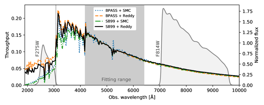
Figure S6: Comparison of stellar population models: Comparison of normalized Starburst99 and bpass models with the Reddy 2016 and SMC dust extinction laws (see Materials and Methods above). The wavelength range used for stellar synthesis fitting is shaded in grey. Also shown are the F725W and F814W throughput curves. The reference model used in this work is the Starburst99 + Reddy 2016 model (black line).

References

- 1. X. Fan, C. L. Carilli, B. Keating, Annual Review of Astronomy and Astrophysics 44, 415 (2006).
- 2. E. Leitet, N. Bergvall, M. Hayes, S. Linné, E. Zackrisson, Astron. Astrophys. 553, A106 (2013).
- 3. Y. I. Izotov, et al., Mon. Not. R. Astron. Soc. (2018).
- 4. Y. I. Izotov, et al., Mon. Not. R. Astron. Soc. 474, 4514 (2018).
- 5. S. Borthakur, T. M. Heckman, C. Leitherer, R. A. Overzier, Science 346, 216 (2014).
- 6. E. Vanzella, et al., Astrophys. J. 825, 41 (2016).
- 7. E. Vanzella, et al., Mon. Not. R. Astron. Soc. 476, L15 (2018).
- 8. A. E. Shapley, et al., Astrophys. J. 826, L24 (2016).
- 9. F. Bian, X. Fan, I. McGreer, Z. Cai, L. Jiang, Astrophys. J. 837, L12 (2017).
- 10. T. J. Fletcher, et al., Astrophys. J. 878, 87 (2019).
- 11. E. Zackrisson, A. K. Inoue, H. Jensen, Astrophys. J. 777, 39 (2013).
- 12. E. C. Herenz, et al., Astron. Astrophys. 606, L11 (2017).
- 13. T. E. Rivera-Thorsen, et al., Astron. Astrophys. 608, L4 (2017).
- 14. J. Chisholm, et al., Astron. Astrophys. 616, A30 (2018).
- 15. A. Bik, et al., Astron. Astrophys. 619, A131 (2018).
- 16. A. Verhamme, I. Orlitová, D. Schaerer, M. Hayes, Astron. Astrophys. 578, A7 (2015).
- 17. M. Dijkstra, M. Gronke, A. Venkatesan, Astrophys. J. 828, 71 (2016).
- 18. C. Behrens, M. Dijkstra, J. C. Niemeyer, Astron. Astrophys. 563, A77 (2014).
- 19. H. Dahle, et al., Astron. Astrophys. 590, L4 (2016).
- 20. Materials and methods are available as supplementary materials.
- 21. A. Adamo, et al., Astrophys. J. 766, 105 (2013).
- 22. K. Vasei, et al., Astrophys. J. 831, 38 (2016).
- 23. T. L. Johnson, et al., Astrophys. J. 843, L21 (2017).
- 24. V. Ramachandran, et al., Astron. Astrophys. 615, A40 (2018).
- 25. J. R. Rigby, M. B. Bayliss, Magellan/MagE observations of the Sunburst Arc, DOI: 10.17045/sthlmuni.9907991 (2019).
- 26. J.-P. Kneib, et al., LENSTOOL: A Gravitational Lensing Software for Modeling Mass Distribution of Galaxies and Clusters (strong and weak regime) (2011).
- 27. J. Chisholm, Sunburst Arch stellar population modeling code, DOI: 10.5281/zenodo.3462663 (2019).
- 28. L. Dressel, Wide Field Camera 3 Instrument Handbook, Version 11.0, Space Telescope Science Institute (2019).
- 29. J. E. Ryon, et al., ACS Instrument Handbook Version 18.0, Space Telescope Science Institute (2019).
- 30. S. Gonzaga, et al., The DrizzlePac Handbook (2012).
- 31. J. L. Marshall, et al., Ground-based and Airborne Instrumentation for Astronomy II (2008), vol. 7014 of Proc. SPIE, p. 701454.
- 32. J. R. Rigby, et al., Astron. J. 155, 104 (2018).
- 33. E. Bertin, S. Arnouts, Astron. Astrophys. Suppl. Ser. 117, 393 (1996).
- 34. S. E. Deustua, et al., UVIS 2.0 Chip-dependent Inverse Sensitivity Values, Tech. rep., Space Telescope Science Institute (2016).
- 35. R. C. Bohlin, Astron. J. 152, 60 (2016).
- 36. C. Leitherer, et al., Astrophys. J. Suppl. Ser. 123, 3 (1999).
- 37. D. F. de Mello, C. Leitherer, T. M. Heckman, Astrophys. J. 530, 251 (2000).
- 38. J. Chisholm, et al., Astrophys. J. 811, 149 (2015).
- 39. C. B. Markwardt, Astronomical Data Analysis Software and Systems XVIII, D. A. Bohlender, D. Durand, P. Dowler, eds. (2009), vol. 411 of Astronomical Society of the Pacific Conference Series, p. 251.
- 40. N. A. Reddy, C. C. Steidel, M. Pettini, M. Bogosavljevic, Astrophys. J. 828, 107 (2016).
- 41. C. Leitherer, et al., Astrophys. J. Suppl. Ser. 189, 309 (2010).
- 42. G. Meynet, A. Maeder, G. Schaller, D. Schaerer, C. Charbonnel, Astron. Astrophys. Suppl. Ser. 103, 97 (1994).
- 43. J. J. Eldridge, et al., Publ. Astron. Soc. Aus. 34, e058 (2017).
- 44. E. R. Stanway, J. J. Eldridge, Mon. Not. R. Astron. Soc. 479, 75 (2018).
- 45. K. D. Gordon, G. C. Clayton, K. A. Misselt, A. U. Land olt, M. J. Wolff, Astrophys. J. 594, 279 (2003).
- 46. D. J. Schlegel, D. P. Finkbeiner, M. Davis, Astrophys. J. 500, 525 (1998).
- 47. J. A. Cardelli, G. C. Clayton, J. S. Mathis, Astrophys. J. 345, 245 (1989).
- 48. J. A. Baldwin, M. M. Phillips, R. Terlevich, Publ. Astron. Soc. Pac. 93, 5 (1981).
- 49. G. Kauffmann, et al., Mon. Not. R. Astron. Soc. 346, 1055 (2003).
- 50. L. J. Kewley, B. Groves, G. Kauffmann, T. Heckman, Mon. Not. R. Astron. Soc. 372, 961 (2006).
- 51. L. J. Kewley, et al., Astrophys. J. 774, 100 (2013).
- 52. J. L. Sérsic, Boletin de la Asociacion Argentina de Astronomia La Plata Argentina 6, 41 (1963).
- 53. J. Chisholm, et al., Astrophys. J. 882, 182 (2019).
- 54. Y. C. Pei, Astrophys. J. 395, 130 (1992).
- 55. L. J. Kewley, M. A. Dopita, R. S. Sutherland, C. A. Heisler, J. Trevena, Astrophys. J. 556, 121 (2001).
- 56. M. R. Blanton, et al., Astron. J. 154, 28 (2017).