Novel Dense Subgraph Discovery Primitives:
Risk Aversion and Exclusion Queries

Abstract

In the densest subgraph problem, given a weighted undirected graph $G(V,E,w)$, with non-negative edge weights $w:E\rightarrow\mathbb{R}$, we are asked to find a subset of nodes $S\subseteq V$ that maximizes the degree density $w(S)/|S|$, where $w(S)$ is the sum of the edge weights induced by $S$. This problem is a well studied problem, known as the densest subgraph problem, and is solvable in polynomial time. But what happens when the edge weights are negative, i.e., $w:E\rightarrow\mathbb{R}$? Is the problem still solvable in polynomial time? Also, why should we care about the densest subgraph problem in the presence of negative weights?

In this work we answer the aforementioned question. Specifically, we provide two novel graph mining primitives that are applicable to a wide variety of applications. Our primitives can be used to answer questions such as “how can we find a dense subgraph in Twitter with lots of replies and mentions but no follows?”, “how do we extract a dense subgraph with high expected reward and low risk from an uncertain graph”? We formulate both problems mathematically as special instances of dense subgraph discovery in graphs with negative weights. We study the hardness of the problem, and we prove that the problem in general is $\mathbf{NP}$-hard. We design an efficient approximation algorithm that works well in the presence of small negative weights, and also an effective heuristic for the more general case. Finally, we perform experiments on various real-world uncertain graphs, and a crawled Twitter multilayer graph that verify the value of the proposed primitives, and the practical value of our proposed algorithms.

The code and the data are available at https://github.com/negativedsd.

1 Introduction

Dense subgraph discovery (abbreviated as DSD henceforth) is a major and active topic of research in the fields of graph algorithms and graph mining. A wide range of real-world, data mining applications rely on DSD including correlation mining, fraud detection, electronic commerce, bioinformatics, mining Twitter data, efficient algorithm design for fast distance queries in massive networks, and graph compression [18].

In this work we introduce two novel primitives for DSD. These two primitives are strongly motivated by real-world applications that we discuss in greater detail in Section 3.1. The first question that our work addresses is related to uncertain graphs. Uncertain graphs appear in a wide variety of applications that we survey in Section 2. We define the uncertain graph model we use formally in Section 3.1, but intuitively, uncertain graphs model probabilistically real-world scenarios where each edge may exist or not in a graph (e.g., failure of a link). Problem 1 aims to find a risk-averse dense subgraph. A similar formulation was suggested recently by Tsourakakis et al. for graph matchings [48].

Our second problem focuses on multigraphs whose edges are associated with different types. Such graphs appear naturally in numerous applications, and are also known as multilayer multigraphs, e.g., [14, 50]. For example, Twitter users may interact in various ways, including follow, reply, mention, retweet, like, and quote. Similarity between two videos can be defined based on different criteria, e.g., audio, visual, and how frequently these videos are being co-watched on Youtube. Similarity between time series can be defined using a variety of measures including Euclidean distance, Fourier coefficients, dynamic time wraping, edit distance among others [20, 43]. Emails between people can be classified bases on the nature of the interaction (e.g., business, family). We formulate Problem 2 whose goal is to detect efficiently dense subgraphs that exclude certain types of edges. Later, we will define two variations of this problem, soft- and hard-exclusion queries.

Contributions. Our contributions are summarized as follows.

• We introduce two novel problems, (i) risk averse DSD, and (ii) DSD in large-scale multilayer networks with exclusion queries. In Section 3.1 we show that these two problems are special cases of DSD in undirected graphs with negative weights. To the best of our knowledge, this is the first work that introduces these algorithmic primitives.

• We prove that DSD in the presence of negative weights is $\mathbf{NP}$-hard in general by reducing Max-Cut to our problem (Section 3.2).

• We design a space-, and time- efficient approximation algorithm that performs best in the presence of small negative weights. In the case of existence of large negative weights, we design a well-performing heuristic.

• We provide an experimental evaluation of our proposed methods on synthetic datasets that illustrate the effect of the parameters in our objective. This understanding allows the practitioner to choose the values of such parameters according to the desired goals of his/her application.

• We deploy our developed primitives on the two real-world applications we introduce. We extract subgraphs from uncertain graphs with high expected induced weight and low risk. Finally, we mine Twitter data by finding dense subgraphs that exclude certain types of interactions. A non-trivial experimental contribution is the creation of an uncertain graph from the TMDB database, and Twitter graphs from the Greek Twitter-verse. Our algorithmic tools provide insights, and we believe that they will find more applications in graph mining, and anomaly detection.

Notation. We use the following notation. Let $deg^{+}(u)>0$ ($deg^{-}(u)$) be the positive (negative) degree of node $u$. Therefore, the total degree of $u$ is $d(u)=deg^{+}(u)-deg^{-}(u)$. Let $w^{+}(e)$ ($w^{+}(e)$) be the positive (negative) edge weight. Finally, $w^{+}(S)$ ($w^{-}(S)$) is the total positive (negative) induced weight by node set $S$, and $d_{S}(u)=deg_{S}^{+}(u)-deg_{S}^{-}(u)$ is the total degree of node $u$ within $S\subseteq V$.

2 Related Work

Uncertain graphs model naturally a wide variety of datasets and applications including protein-protein interactions [3, 30], kidney exchanges [41], influence maximization [26], and privacy-applications [4]. While a lot of research work has focused on designing graph mining algorithms for uncertain graphs [6, 23, 27, 29, 33, 36, 37, 38], there is less work on designing efficient risk-averse optimization algorithms, and even lesser with solid theoretical guarantees.

Risk-aversion has been implicitly discussed by Lin et al. in their work on reliable clustering [33], where the authors show that interpreting probabilities as weights does not result in good clusterings. Repetitive sampling from a large-scale uncertain graph in order to reduce the risk is inefficient. Motivated by this observation, Parchas et al. have proposed a heuristic to extract a good possible world in order to combine risk-aversion with efficiency [37]. However, their work comes with no guarantees. Jin et al. provide a risk-averse algorithm for distance queries on uncertain graphs [24]. He and Kempe propose robust algorithms for the influence maximization problem [22]. Since then, various extensions have been proposed for the same problem [11, 49]. Closest to our work lies the recent work by Tsourakakis et al. who proposed efficient approximation algorithms for finding risk-averse heavy matchings in uncertain graphs and hypergraph [48].

Dense subgraph discovery (DSD) is a major topic of research in the fields of graph algorithms and graph mining, with many diverse applications, ranging from fraud detection to bioinformatics, see [18] for a detailed account of such applications. Finding cliques [25], or optimal quasi-cliques [45, 46, 44] is the prototypical DSD formulations but not only they are $\mathbf{NP}$-hard problems, but also hard to approximate [21]. On the contrary, the densest subgraph problem (DSP) is solvable in polynomial time [16, 19]. The DSP for undirected, weighted graphs $G(V,E,w),w:E\rightarrow\mathbb{R}^{+}$ maximizes the degree density $\rho(S)=\frac{w(S)}{|S|}$ over all possible subgraphs $S\subseteq V$, where $w(S)=\sum_{e\in e[S]}w(e)$ is the total induced weight by subgraph. In addition to the exact algorithm that is based on maximum flow computation, Charikar [8] proved that the greedy algorithm proposed by Asashiro et al. [2] produces a $\frac{1}{2}$-approximation of the densest subgraph in linear time. Both algorithms are efficient in terms of running times and scale to large networks. In the case of directed graphs, the densest subgraph problem is solved in polynomial time as well. Charikar [8] provided a linear programming approach which requires the computation of $n^{2}$ linear programs and a $\frac{1}{2}$-approximation algorithm which runs in $O(n^{3}+n^{2}m)$ time. Khuller and Saha [28] improved significantly the state-of-the art by providing an exact combinatorial algorithm and a fast $\frac{1}{2}$-approximation algorithm which runs in $O(n+m)$ time. Since then, many variations of the densest subgraph problem have been proposed in the literature. Tsourakakis generalized the DSP the the $k$-clique DSP that maximizes the average density of $k$-cliques, and also provided efficient exact and approximation algorithms [47], see also [34]. Another interesting set of variations of the DSP across a set of graphs was introduced by Semertzidis et al. [42], and was analyzed further by Charikar et al. [9]. Finally, the densest subgraph problem with exclusion queries on multilayer graphs has not been considered before. Galimberti et al. studied core decompositions – a concept intimately connected to DSD– on multilayer graphs [15]. Finally, Cadena et al. first studied DSD with negative weights [7], but their work focuses on anomaly detection, and the streaming nature of their input.

DSD on uncertain graphs is a less well studied topic. Zou was the first who discussed the DSP on uncertain graphs. His work shows –as expected– that the DSP in expectation can be solved in polynomial time [51]. The closest work related to our formulation is the recent work by Miyauchi and Takeda [35]. While their original motivation is also DSD on uncertain graphs, the modeling assumptions, and the mathematical objective differ significantly from ours. To the best of our knowledge, there is no work on risk-averse DSD under general probabilistic assumptions as ours.

3 Proposed Method

3.1 Why Negative Weights?

Risk-averse dense subgraph discovery. Uncertain graphs model the inherent uncertainty associated with graphs in a variety of applications, that we discussed earlier in detail, see Section 2. Here, we adopt the general model for uncertain graphs introduced by Tsourakakis et al. [48]. For completeness we present it in the following.

Model: Let $\mathcal{G}([n],E,\{f_{e}(\theta_{e})\}_{e\in E})$ be an uncertain complete graph on $n$ nodes, with the complete edge set $E={[n]\choose 2}$. The weight $w(e)$ (reward) of each edge $e\in E$ is drawn according to some probability distribution $f_{e}$ with parameters $\vec{\theta_{e}}$, i.e., $w(e)\sim f_{e}(x;\vec{\theta_{e}})$. We assume that the weight of each edge is drawn independently from the rest; each probability distribution is assumed to have finite mean, and finite variance. Given this model, we define the probability/likelihood of a given graph $G$ with weights $w(e)$ on the edges as:

$${\bf{Pr}}\left[{G;\{w(e)\}_{e\in E}}\right]=\prod_{e\in E}f_{e}(w(e);\vec{\theta_{e}}).$$ (1)

This model includes the standard Bernoulli model that is used extensively in the existing literature as a special case. Specifically, in the standard binomial uncertain graph model an uncertain graph is modeled by the triple $\mathcal{G}=(V,E,p)$ where $p:E\rightarrow(0,1]$ is the function that assigns a probability of success to each edge independently from the other edges. According to the possible-world semantics [5, 13] that interprets $\mathcal{G}$ as a set $\{G:(V,E_{G})\}_{E_{G}\subseteq E}$ of $2^{|E|}$ possible deterministic graphs (worlds), each defined by a subset of $E$. The probability of observing any possible world $G(V,E_{G})\in 2^{E}$ is

$${\bf{Pr}}\left[{G}\right]=\prod\limits_{e\in E_{G}}p(e)\prod\limits_{e\in E\backslash E_{G}}(1-p(e)).$$

A key observation to hold in mind, is that each edge $e$ in the uncertain graph is independently distributed from the rest and is associated with an expected reward $\mu_{e}$ (expectation) and a risk $\sigma_{e}^{2}$ (variance). Finally, observe that without any loss of generality in our general model described by equation (1) we have assumed that the edge set is ${[n]\choose 2}$; non-edges can be modeled as edges with probability of existence zero.

Algorithm 1 Exclusion-Queries$(G(V,E),\{\text{colors}\},W>0)$

  for $e\in E(G)$ do

     for $c\in\text{colors}$ do

        if If $type(e)=c$ then

           $w(e)\leftarrow-W$ (else $w(e)$ remains 1)

        end if

     end for

  end for

  Return $S\subseteq V$ that achieves maximum average degree in $G(V,E,w)$.

Problem formulation. Intuitively, our goal is to find a subgraph $G[S]$ induced by $S\subseteq V$ such that its average expected reward $\frac{\sum\limits_{e\in E(S)}w_{e}}{|S|}$ is large and the associated average risk is low $\frac{\sum\limits_{e\in E(S)}\sigma_{e}^{2}}{|S|}$. To achieve this purpose we model the problem as a densest subgraph discovery problem in a graph with positive (reward) and negative (risk) edge weights. Specifically, for every edge $e=(u,v)\in E(G)$ we create two edges, a positive edge with weight equal to the expected reward, i.e., $w^{+}(e)=\mu_{e}$ and a negative edge with weight equal to the opposite of the risk of the edge, i.e., $w^{-}(e)=\sigma_{e}^{2}$. We wish to find a subgraph $S\subseteq V$ that has large positive average degree $\frac{w^{+}(S)}{|S|}$, and small negative average degree $\frac{w^{-}(S)}{|S|}$. We combine the two objectives into one objective $f:2^{V}\rightarrow\mathbb{R}$ that we wish to maximize:

$$f(S)=\frac{w^{+}(S)+\lambda_{1}|S|}{w^{-}(S)+\lambda_{2}|S|}.$$

The parameters $\lambda_{1},\lambda_{2}\geq 0$ are positive reals. First, observe that this dense subgraph discovery formulation is applicable to any graph with positive and negative weights. Parameters $\lambda_{1},\lambda_{2}$ allow us to control the size of the output as follows. Let us reparameterize the two parameters as $\lambda_{1}=\rho\lambda,\lambda_{2}=\lambda$. Then $f(S)=\frac{w^{+}(S)+\rho\lambda|S|}{w^{-}(S)+\lambda|S|}$, so if the ratio $\rho\geq 1$, then the objective favors larger node sets, whereas when $\rho<1$ we favor smaller node sets.

We show how to solve the problem $\max\nolimits_{S\subseteq V}f(S)$ by reducing it to standard dense subgraph discovery [32, 19]. We perform binary search on $f(S)$ by answering queries of the following form:

Does there exist a subset of nodes $S\subseteq V$ such that $f(S)\geq q$, where $q$ is a query value?

Assuming an efficient algorithm for answering this query, and that the weights are polynomial functions of $n$, then using $O(\log n)$ queries we can find the optimal value for our objective $f:V\rightarrow\mathbb{R}$. By analyzing what each query corresponds to, we find:

$$\frac{w^{+}(S)+\lambda_{1}|S|}{w^{-}(S)+\lambda_{2}|S|} \geq q\rightarrow w^{+}(S)+\lambda_{1}|S|\geq q(w^{-}(S)+\lambda_{2}|S|)\rightarrow$$ (2)

$$\sum_{e\in E(S)}\underbrace{\bigg{(}w^{+}(e)-qw^{-}(e)\bigg{)}}_{\tilde{w}(e)} \geq|S|\underbrace{(q\lambda_{2}-\lambda_{1})}_{q^{\prime}}\rightarrow\sum_{e\in E(S)}\frac{\tilde{w}(e)}{|S|}\geq q^{\prime}.$$

The latter inequality suggests that our original problem corresponds to querying in $\tilde{G}$ –a modified version of $G$ where the edge weight of any edge $e$ becomes $w^{+}(e)-qw^{-}(e)$– whether there exists a subgraph $S$ with density greater than $q^{\prime}$, where $q^{\prime}=q\lambda_{2}-\lambda_{1}$. However, this does not imply that our problem is poly-time solvable. The densest subgraph problem is poly-time solvable using a maximum flow formulation when the weights are positive rationals [19]. As we will prove in the next section, the densest subgraph problem when there exist negative weights is $\mathbf{NP}$-hard in general. However, our analysis above leads to a straight-forward corollary that is worth stating. Intuitively, when for each edge $e$ the ratio $\frac{w^{+}(e)}{w^{-}(e)}$ is large enough, then our problem is solvable in polynomial time.

Corollary 1.

Assume that $w^{+}(e)\geq q_{max}w^{-}(e)$ for all $e\in E^{+}\cup E^{-}$, where $q_{max}$ is the maximum possible query value. Then, the densest subgraph problem is solvable in polynomial time.

Proof.

If $w^{+}(e)\geq q_{max}w^{-}(e)$ for each $e\in E$, we obtain $\tilde{w}(e)\geq 0$ for each $e\in E$ in inequality (2) is equivalent to solving the densest subgraph problem in an undirected graph with non-negative weights, see [19, 47]. ∎

Observe that a trivial upper bound of $q_{\max}$ can be obtained by setting $w^{+}(S)=\sum_{e\in E(G)}w^{+}(e),w^{-}(S)=0$, and since $\lambda_{1}|S|\leq\lambda_{1}n,\lambda_{2}|S|\geq\lambda_{2}$ for all $S\neq\emptyset$, we see that $q_{\max}\leq\frac{\sum_{e\in E(G)}w^{+}(e)+\lambda_{1}n}{\lambda_{2}}$. For polynomially bounded weights, this is a polynomial function of $n$, hence the number of binary search iterations is logarithmic.

Controlling the risk in practice. There exist real-world scenarios where the practitioner wants to control the trade-off between reward and risk, see [48]. An effective way to change the risk tolerance is as follows by multiplying the negative induced weight $w^{-}(S)$ by $B\in(0,+\infty)$. Namely, our objective $f:2^{V}\rightarrow\mathbb{R}$ is $f(S)=\frac{w^{+}(S)+\lambda_{1}|S|}{Bw^{-}(S)+\lambda_{2}|S|}.$ An interesting open problem is to develop a formal (bi-criteria) approximation for risk averse DSD along the lines of [40, 48].

Soft and hard exclusion dense subgraph queries. Given the Twitter network, where user accounts may interact in more than one ways (e.g., follow, retweet, mention, quote, reply), can we find a dense subgraph that does not contain any follow but contains many reply interactions? We ask this question in a more general form.

We consider two types of such queries. The soft and hard queries. In the former case we want to find subgraphs with perhaps few edges of certain types, in the latter case we want to exclude fully such edges. An algorithmic primitive that can answer efficiently these queries can be used to understand the structure of large-scale multilayer networks, and find anomalies and interesting patterns. As a result, subgraphs that do not induce any edge of any excluded type will have positive weight, whereas subgraphs that induce even one edge of a forbidden type will have $-\infty$ weight. In principle, we set the edge weight of an excluded type to $-W$ where $W>0$ is an input parameter. The pseudo-code in Algorithm shows this approach. Again, dense subgraph discovery with negative weights plays the key role in developing such a graph primitive. In practice, a practitioner may range $\kappa$ from small to large values.

3.2 Hardness

We prove that solving the densest subgraph problem on graphs with negative weights is $\mathbf{NP}$-hard. We formally define our problem Neg-DSD.

We prove that Neg-DSD is $\mathbf{NP}$-hard. Our reduction is based on the the proposed strategy by Peter Shor for showing that the max-cut problem on graphs with possibly negative edges is $\mathbf{NP}$-hard [1]. This is stated as the Theorem 1.

Theorem 1.

Neg-DSD is $\mathbf{NP}$-hard.

For convenience, we define the decision version of the maximum cut problem [1].

Problem (Max-Cut).

Given a graph $G(V,E)$ and a constant $c$, find a partition $(A,B)$ of $V$ such that $cut(A,B)>c$.

Our proof strategy is inspired by Peter Shor’s proof that max-cut with negative weight edges is $\mathbf{NP}$-hard [1]. We provide a detailed proof sketch of Theorem 1.

Proof.

First, we define the Positive-Cut problem, and show that it is $\mathbf{NP}$-hard by reducing the Max-Cut problem to it.

Problem (Positive-Cut).

Given a graph $G$ with possibly negative weights, find a partition $(A,B)$ of $V$ such that $cut(A,B)>0$.

We choose two nodes $u,v$ that lie on opposite sides of an optimal max cut $(A^{*},B^{*})$. Despite the fact we do not know the max cut, we can perform this step in polynomial time by repeating the following procedure for all possible pairs of nodes; if we cannot find a positive cut for any of the pairs, then the answer to the Max-Cut is negative. We construct a graph $G^{\prime}$ by adding a very large negative weight equal to $-d$ from $u$ and $v$ to all other vertices, and an edge of weight $(n-2)d-c$ between $u,v$. All cuts that place $u,v$ on the same side will be negative in $G^{\prime}$ provided $d$ is sufficiently large. All other cuts will be positive if and only if the corresponding cut in $G$ is greater than $c$. Therefore, Positive-Cut is $\mathbf{NP}$-hard.

Finally we prove that Neg-DSD is $\mathbf{NP}$-hard using a reduction from Positive-Cut. We construct a graph $G^{\prime}$ by negating every weight in $G$ putting a loop on every vertex so that its weighted degree is zero. Hence the sum of the degrees of any set $A$ in $G^{\prime}$ is equal to $0=\sum_{v\in S}0=2w(A)+cut(A,\bar{A})$. Observe that a cut $(A,B)$ has positive weight in $G$ if and only if $A$ has positive average degree. This completes the proof. ∎

3.3 Algorithms and Heuristics

A popular algorithm for the densest subgraph problem is Charikar’s algorithm [8]. We study the performance of this algorithm in the presence of negative weights. The pseudocode is given as Algorithm 2. The algorithm iteratively removes from the graph the node of the smallest degree $d(v)=deg^{+}(v)-deg^{-}(v)$, and among the sequence of $n$ produced graphs, outputs the one that achieves the highest degree density. Our main theoretical result for the performance of Algorithm 2 is stated as Theorem 2.

Algorithm 2 Peeling$(G)$

  $n\leftarrow|V|,H_{n}\leftarrow G$

  for $i\leftarrow n$ to $2$ do

     Let $v$ be the vertex of $G_{i}$ of minimum degree, i.e., $d(v)=deg^{+}(v)-deg^{-}(v)$ (break ties arbitrarily)

     $H_{i-1}\leftarrow H_{i}\backslash{v}$

  end for

  Return $H_{j}$ that achieves maximum average degree among $H_{i}$s, $i=1,\ldots,n$.

Theorem 2.

Let $G(V,E,w)$, $w:E\rightarrow\mathbb{R}$ be an undirected weighted graph with possibly negative weights. If the negative degree $deg^{-}(u)$ of any node $u$ is upper bounded by $\Delta$, then Algorithm 2 outputs a set whose density is at least $\frac{\rho^{*}}{2}-\frac{\Delta}{2}$.

Proof.

Let $S^{*}$ be the optimal densest subgraph in $G$ with average density $\frac{w(S^{*})}{|S^{*}|}=\rho^{*}$. By the optimality of $S^{*}$ we obtain that $d_{S^{*}}(v)\geq\rho^{*}$, and then trivially $deg^{+}(v)\geq\rho^{*}$. Consider the execution of algorithm 2, and let $u\in S^{*}$ be the first vertex from $S^{*}$ removed during the peeling. Let $S$ be the set of nodes at that iteration, including $u$. By the peeling process, we have $d_{S}(v)\geq d_{S}(u)$ for all $v\in S$. Furthermore,

$$d_{S}(u)=deg_{S}^{+}(u)-deg_{S}^{-}(u)\geq\deg_{S}^{+}(u)-\Delta,$$

since by our assumption $deg_{S}^{-}(u)\leq deg^{-}(u)\leq\Delta$. This implies that

$$2w(S) =\sum\limits_{v\in S}d_{S}(v)\geq\sum\limits_{v\in S}deg_{S}^{+}(v)-|S|\Delta\geq|S|(\rho^{*}-\Delta)\rightarrow\frac{w(S)}{|S|}\geq\frac{\rho^{*}}{2}-\frac{\Delta}{2}.$$

This yields that the output of Algorithm 2 outputs a subgraph $H$ with degree density at least $\frac{\rho^{*}}{2}-\frac{\Delta}{2}$. ∎

When the additive error term in the approximation is small compared to the term $\frac{\rho^{*}}{2}$, then the peeling algorithm performs effectively. In practice, Algorithm 2 performs well on large-scale graphs where the negative weights are small. In the presence of large negative degrees, the approximation guarantees become less meaningful, or even meaningless.

Claim.

In the presence of large negative weights, Algorithm 2 may perform arbitrarily bad.

This is illustrated in Figure 1($\alpha$) that provides a bad graph instance with $n+4$ nodes for our proposed algorithm. Let $W=\frac{n-4}{3}$. Then, $3W-n<-3$. The degrees of the $n+4$ nodes are as follows:

$$\underbrace{3W-n}_{\text{one node}}<\underbrace{-3}_{n-2\text{~{}nodes}}<\underbrace{-2}_{\text{two nodes}}<0<\underbrace{2\epsilon+W}_{\text{three nodes}}.$$

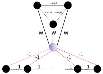
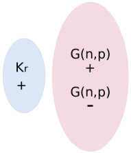
($\alpha$)		($\beta$)

Figure 1: Bad peeling instances. For details, see Section 3.

Therefore, the center node is removed first, and the peeling algorithm will output as the densest subgraph the triangle of density $\epsilon$. The optimal densest subgraph has $\frac{3W+3\epsilon}{4}$. By allowing $\epsilon$ to be arbitrarily small, we observe that the approximation ratio becomes arbitrarily bad. To tackle such scenarios, i.e., where nodes from the densest subgraph are peeled earlier than when they should, we propose an effective heuristic which is outlined in Algorithm 3. The algorithm again peels the nodes but scores every node $u$ according to $Cdeg^{+}{(u)}-deg^{-}{(u)}$, where $C>0$ is a parameter that is part of the input.

Remark about $C$ in Algorithm 3. While Figure 1($\alpha$) suggests the use of $C\geq 1$, it could be the case that $C$ has to be set to a value less than 1 to obtain good results. We provide an example where using $C<1$ can help in providing a better peeling permutation of the nodes. Consider a graph whose weights are either $+1$ or $-1$, that consists of two connected components. The first component is a positive clique on $r$ nodes. The second component is the union of two random binomial graphs $G(n,p)$ where $p=\frac{1}{2}$. This is illustrated in Figure 1($\beta$). The degree of any node $u$ in the first component is $deg(u)=deg^{+}(u)-deg^{-}(u)=(r-1)-0$. The expected degree of any node in the second component is 0. Furthermore, the average degree of any subset of nodes in the 2nd component is 0 in expectation. However, using concentration bounds (details omitted) one can show that it is likely that there will exist a node $u$ in the second component with positive degree $\kappa\sqrt{n}$ and negative degree $\kappa^{\prime}\sqrt{n}$ with $\kappa>\kappa^{\prime}$, and therefore positive total degree. Only the use of a $C<1$ will improve the peeling ordering; for example one can immediately see that in the extreme case where $C=0$ the nodes of the second component will be removed first.

Rule-of-thumb. In practice, given that each run of the algorithm takes linear time, we can afford to run the algorithm for a bunch of $C$ values and return the densest subgraph among the outputs produced by each run, instead of using one value for $C$. This strategy is applied in Section 4.

Algorithm 3 Heuristic-Peeling$(G,C)$

0:  $C\in(0,+\infty)$

  $n\leftarrow|V|,H_{n}\leftarrow G$

  for $i\leftarrow n$ to $2$ do

     Let $v$ be the vertex of $G_{i}$ of minimum degree, i.e., $d(v)=Cdeg^{+}(v)-deg^{-}(v)$ (break ties arbitrarily)

     $H_{i-1}\leftarrow H_{i}\backslash{v}$

  end for

  Return $H_{j}$ that achieves maximum average degree among $H_{i}$s, $i=1,\ldots,n$.

Shifting the negative weights. Finally, for the sake of completeness, we mention that the perhaps natural idea of shifting all the weights by the most negative weight in the graph, in order to obtain non-negative weights, and apply the exact polynomial time algorithm on the weight-shifted graph may perform arbitrarily bad. To see why, consider a graph on $n+5$ nodes that consists of three components, a triangle with positive weights equal to 1, an edge with a large negative weight $-\Delta<0$, and a large clique on $n$ nodes, whose each edge weight is equal to $-\epsilon<0$. In this graph, the densest subgraph is the positive triangle. However, shifting the weights by $+\Delta$, the degree density of the triangle becomes $1+\Delta$, and of the clique $\frac{{\Delta-\epsilon\choose 2}}{n}$. For large enough $\Delta$, assuming $\epsilon$ is negligible, the densest subgraph is the clique whose true degree density is negative. Also experimentally, this heuristic performs extremely poorly.

4 Experimental results

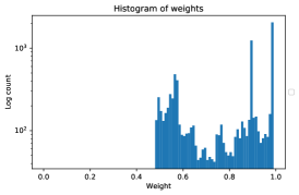
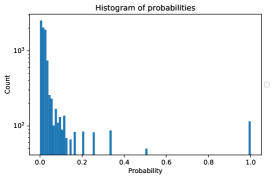
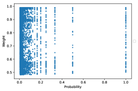
($\alpha$)	($\beta$)	($\gamma$)
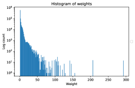
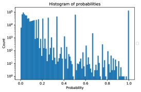
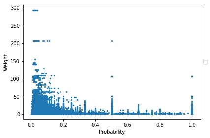
($\delta$)	($\epsilon$)	($\sigma\tau$)

Figure 2: Uncertain graph statistics. First and second rows correspond to Collins and TMDB datasets respectively. ($\alpha$),($\delta$) Log histogram of weights. ($\beta$),($\epsilon$) Log histogram of edge probabilities. ($\gamma$),($\sigma\tau$) Scatterplot of weights vs. edge probabilities.

Name	$n$	$m$
$\blacksquare$ Biogrid	5 640	59 748
$\blacksquare$ Collins	1 622	9 074
$\blacksquare$ Gavin	1 855	7 669
$\blacksquare$ Krogan core	2 708	7 123
$\blacksquare$ Krogan extended	3 672	14 317
$\odot$ TMDB	160 784	883 842
$\odot$ Twitter (Feb. 1)	621 617	(902 834, 387 597, 222 253, 30 018, 63 062)
$\odot$ Twitter (Feb. 2)	706 104	(1 002 265, 388 669, 218 901, 29 621, 64 282)
$\odot$ Twitter (Feb. 3)	651 109	(1 010 002, 373 889, 218 717, 27 805, 59 503)
$\odot$ Twitter (Feb. 4)	528 594	(865 019, 435 536, 269 750, 32 584, 71 802)
$\odot$ Twitter (Feb. 5)	631 697	(999 961, 396 223, 233 464, 30 937, 66 968)
$\odot$ Twitter (Feb. 6)	732 852	(941 353, 407 834, 239 486, 31 853, 67 374)
$\odot$ Twitter (Feb. 7)	742 566	(1 129 011, 406 852, 236 121, 30 815, 68 093)

Table 1: Datasets used in our experiments. The number of vertices $n$ and edges $m$ is recorded for each graph. The datasets annotated by $\odot$ have been created by us, and are publicly available. The five-dimensional vector containing the number of edges for each day of Twitter correspond to follow, retweet, mention, quote, reply respectively. For details, see Section 4.1.

4.1 Experimental setup

Datasets. The datasets we have used in our experiments are shown in Table 1. We use five uncertain graphs, Biogrid, Collins, Gavin, Krogan core, Krogan extended that have been used in prior biological studies (e.g., [12, 17, 30]), and are available at [31], and one uncertain graph that we created from the TMDB movie database as follows, and is available at [10]. The set of nodes corresponds to actors, and the probability of the edge is equal to the probability that these two actors co-star in a movie. Specifically, for actors $u,v$, the probability $p(u,v)$ is equal to the Jaccard coefficient $J(M_{u},M_{v})=\frac{|M_{u}\cap M_{v}|}{|M_{u}\cup M_{v}|}$, where $M_{u},M_{v}$ are the sets of movies that $u,v$ have co-starred respectively. We choose weights to represent a function of the popularity of the movies, i.e., a score assigned to each movie by TMDB. Intuitively, these scores reflect the reward of a potential collaboration between two actors. While there are many ways to set the weight of an edge for two actors (e.g. average popularity), we focus on the most popular movies they have co-starred in. The main rationale behind this choice is that the majority of actors play in movies whose majority popularity is 1, i.e., the lowest possible. For a pair of actors $\{u,v\}$, let $s_{0}\geq\ldots\geq s_{k-1}$ where $k=\min(|M_{u}\cap M_{v}|,5)$ be the popularity scores of movies they have co-starred in. We set $w(u,v)=\sum_{j=0}^{k-1}\frac{s_{j}}{2^{j}}$, i.e., a discounted sum of popularities, focusing more on the most popular movies the two actors have co-starred in.

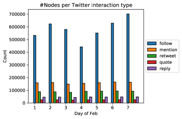
($\alpha$)	($\beta$)

Figure 3: ($\alpha$) Count of Twitter accounts per day, and ($\beta$) count of Twitter interactions for the first week of February 2018, involved in five types of interactions.

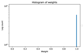
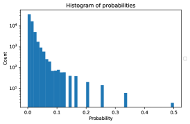
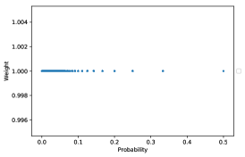
($\alpha$)	($\beta$)	($\gamma$)
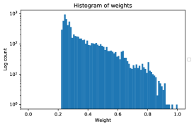
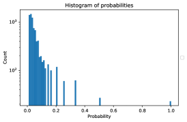
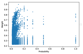
($\delta$)	($\epsilon$)	($\sigma\tau$)
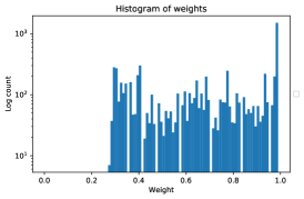
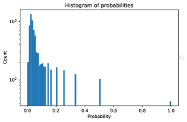
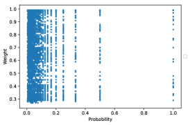
($\zeta$)	($\eta$)	($\theta$)
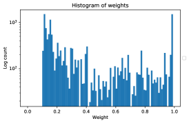
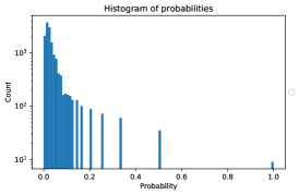
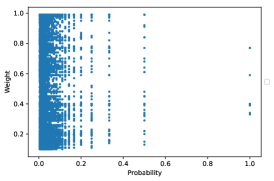
($\iota$)	($\iota\alpha$)	($\iota\beta$)

Figure 7: Uncertain graphs’ statistics. Each row corresponds to biogrid, gavin, krogan, krogan extended respectively. First and second column show histograms of weights and edge probabilities respectively. The third column shows the scatterplot among the latter quantities.

Figure 2 provides a detailed view of basic properties of two of the uncertain graphs we use in our experiments. The first and second row correspond to the Collins and TMDB datasets respectively. The first and second columns show the histograms of the weights and edge probabilities in log-scale, and the third column provides a scatter-plot of edge weights versus edge probabilities. The same results for the rest of the uncertain graphs appears in Figure 7 in the Appendix 6. Finally, we used an open-source twitter API crawler to monitor twitter traffic between February 1st and February 14th, 2018 [39]. We provide detailed information about each daily graph. Here, the number of edges is a five dimensional vector, whose coordinates correspond to the number of follows, mentions, retweets, quotes, and replies. Figure 3 shows these counts. Specifically, Figure 3($\alpha$) shows the number of Twitter accounts (nodes) involved in five types of Twitter interactions, follow, retweet, mention, quote, and reply for the first seven days of February 2018. The total number of nodes involved in all interactions is shown in Table 1. Similarly, Figure 3($\beta$) shows the number of Twitter interactions per type. The follow interactions are the majority for each day, and the mention interaction comes second for each day too. The datasets we use are overall small, and medium sized, therefore our proposed algorithm for a fixed $C$ value, requires few seconds or few minutes for the largest graphs.

Machine specs and code. The experiments were performed on a single machine, with an Intel Xeon CPU at 2.83 GHz, 6144KB cache size, and 50GB of main memory. The code is written in Python, and is available at https://github.com/negativedsd.

4.2 Risk-averse DSD

$B$	Average exp. reward	average risk	$|S^{*}|$
0.25	0.18	0.09	6
1	0.17	0.08	10
2	0.13	0.06	31

Table 2: Exploring the effect of risk tolerance parameter $B$ on the gavin dataset. For details, see Section 4.2.

We perform two risk averse DSD experiments. First, for various fixed pairs of ($\lambda_{1},\lambda_{2})$ values, we range the parameter $B$ (reminder: $B$ is the multiplicative factor of $w^{-}(S)$, see Controlling the risk in practice, Section 3.1) to control the trade-off between expected average reward and average risk. A typical outcome of our algorithm on the set of uncertain graphs we have tested it on for $\lambda_{1}=\lambda_{2}=1$, and $C=1$ is summarized in Table 2. As $B$ increases, we tolerate less risk, and the average expected reward drops. This shows the trade-off between expected reward and risk.

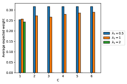
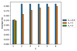
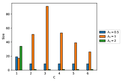
($\alpha$)	($\beta$)	($\gamma$)
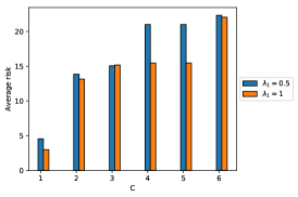
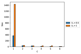
($\delta$)	($\epsilon$)	($\sigma\tau$)

Figure 4: Risk averse DSD results for Collins ($\alpha$) average expected weight, ($\beta$) average risk, ($\gamma$) output size, and for TMDB ($\delta$) average expected weight, ($\epsilon$) average risk, ($\sigma\tau$) output size. For details, see Section 4.2.

In our second experiment we test the effect of rest of the parameters. We fix $B=1$, and then we perform the following procedure. For each dataset, we fix a pair of $(\lambda_{1},\lambda_{2})$ values and run our proposed algorithm using 7 values of $C$. The $C$ value $0.5$ always resulted in trivial results that would skew a lot the plots so it is omitted. Specifically, for $C=0.5$ for all three pairs of $\lambda$ values we use, we obtain (almost) the whole graph as output of the peeling process. The three pairs of $\lambda$ values we use are $(\lambda_{1},\lambda_{2})\in\{(0.5,1),(1,1),(2,1)\}$. Our results are shown in Figure 4 for the Collins and the TMDB graphs respectively. We remark that for the TMDB graph, the last pair of $\lambda$ values $(2,1)$ results in obtaining the whole graph as the optimal solution, so we omit it from the plots in Figures 4($\delta$),($\epsilon$), and ($\sigma\tau$), see also Figure 8 ($\iota\gamma$), ($\iota\delta$), and ($\iota\epsilon$) for the complete results. Changing $C$ value in principle does not affect risk aversion (e.g., Figure 4($\beta$)), but in some cases due to the different peeling orderings that different $C$ values yield the output may be associated with different risks (e.g., Figure 4)($\delta$)). We also observe that as we increase $\lambda_{1}$ the size of the output increases. This agrees with the insights we provide in Section 3; namely, we reward larger sets of nodes. The results for the rest of the datasets are included in the Appendix 6.

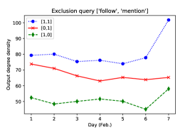
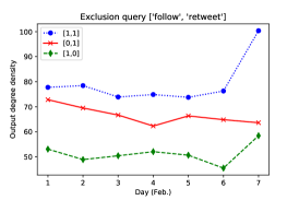
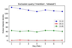
($\alpha$)	($\beta$)	($\gamma$)
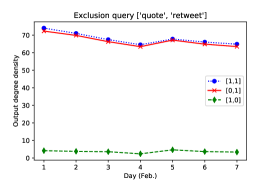
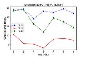
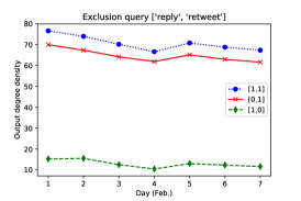
($\delta$)	($\epsilon$)	($\sigma\tau$)

Figure 5: Degree density for three exclusion queries per each pair of interaction types over the period of the first week of February 2018. ($\alpha$) Follow and mention. ($\beta$) Follow and retweet. ($\gamma$) Mention and retweet. ($\delta$) Quote and retweet. ($\epsilon$) Reply and quote. ($\sigma\tau$) Reply and retweet.

4.3 Mining Twitter using DSD-Exclusion queries

We test our DSD exclusion query primitive on the Twitter daily data. We present results that we obtain for different pairs of graphs induced by different types of interactions, for $C=1$. For each such pair, we all possible non-trivial exclusion queries:

• Every type of interaction is allowed (query denoted as $[1,1]$).

• One of the two interaction types is excluded (queries denoted as $[1,0]$, and $[0,1]$).

Figures 5, 6 show for each pair of interactions the degree density, and the size (i.e., number of nodes) of the output. Interestingly, observe that in Figure 6($\gamma$) the exclusion query $[0,1]$ that excludes mentions and allows retweets results in density close to 0. This is because the Twitter API considers every retweet as a mention. By excluding mentions, we exclude all retweets! The density is not zero, due to some small noise in the crawled mentions, i.e., there exist a few retweets that have not been included in the mentions.

We have performed more exclusion queries that involve more types of interactions. For instance, by looking into reply, quote, retweet interactions, we find the following results for two queries on February 1st, 2018.

• When we allow all types we find a subset of 351 nodes, whose retweet density is 72.6, reply density 3.86, and quote density 1.08. We observe this difference since the retweet layer of interactions is much denser than the other two.

• When we exclude the retweets, but allow quotes and replies, we find a set of 30 nodes whose reply degree density is 15.46, and quote degree density 0.066.

Effect of $C$, and $W$. As we discussed earlier, ranging $W$, from small values to $+\infty$ quantifies how much we care about excluding the undesired edge types. Table 3 shows what we observe typically on all experiments we have performed. Specifically, we perform an exclusion query $[1,0]$ on the retweet, reply interactions. We denote by $S^{*}$ the output of Algorithm 3. By inspecting the last column $\rho_{\text{reply}}(S^{*})$ of the table, we observe that even when we set the weight of each reply interaction to -1 (soft query), our algorithm outputs a set $S^{*}$ with very few replies, for all $C\in\{\frac{1}{10},1,10\}$ values we use. When $W$ is set to the very large value $200\,000$ (hard query), $\rho_{\text{reply}}(S^{*})$ becomes 0 but we also observe a drop in the degree density of the retweets. For instance for $C=1$, $\rho_{\text{retweet}}(S^{*})$ drops from 72.70 to 30.38.

$C$	$W$	$|S^{*}|$	$\rho_{\text{retweet}}(S^{*})$	$\rho_{\text{reply}}(S^{*})$
$0.1$	1	296	63.44	-0.75
	5	99	45.67	-0.01
	200 000	200	30.37	0
$1$	1	346	72.70	-2.75
	5	319	68.70	-1.29
	200 000	200	30.38	0
$10$	1	351	73.10	-3.31
	5	351	73.10	-3.31
	200 000	200	30.37	0

Table 3: Exploring the effect of the negative weight $-W$ on the excluded edge types for various $C$ values. For details, see Section 4.3.

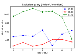
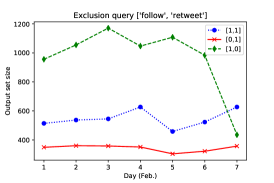
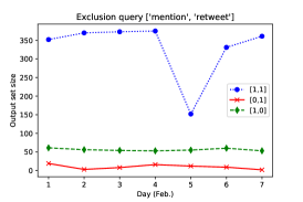
($\alpha$)	($\beta$)	($\gamma$)
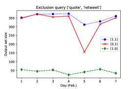
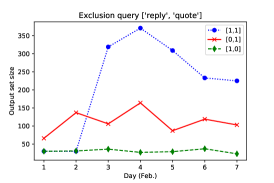
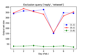
($\delta$)	($\epsilon$)	($\sigma\tau$)

Figure 6: Output sizes for three exclusion queries per each pair of interaction types over the period of the first week of February 2018. ($\alpha$) Follow and mention. ($\beta$) Follow and retweet. ($\gamma$) Mention and retweet. ($\delta$) Quote and retweet. ($\epsilon$) Reply and quote. ($\sigma\tau$) Reply and retweet.

5 Conclusion

Summary. In this paper we study dense subgraph discovery problem on graphs with negative weights in greater depth than prior work [7]. We show that the problem in $\mathbf{NP}$-hard, and then we propose algorithms that are based on peeling, and are both space-, and time-efficient. Furthermore, we provide two important graph mining primitives, that are both formalized as Neg-DSD problems. The first primitive is applicable to uncertain graphs, and extracts subgraphs that in expectation induce large weight, and are risk-averse. The second primitive enables for efficient mining of multilayer graphs; specifically, it extracts dense subgraphs that exclude certain types of undesired edges, that are passed as input to the algorithm. Given the ubiquitousness of uncertain and multilayer graphs, and the importance of DSD [18], we believe that our primitives will be applied on various applications. Finally, we test our proposed methods on various real-world datasets, and verify experimentally their usefulness and efficiency.

Open Problems. While we have performed some work on understanding the computational complexity of the problem, understanding at a greater depth the complexity (especially under reasonable assumptions on the negative weights) of the problem remains largely open. For example, we provided sufficient conditions under which the problem is poly-time solvable. What are necessary and sufficient conditions for poly-time solvability of the DSP on graphs with negative edge weights? Furthermore, using our primitives on more applications is an interesting direction (e.g., mining time-series; for example, can we find clusters of time-series that are correlated under one similarity measure but not correlated under similarity a second similarity measure?). Also, developing an approximation or bi-criteria approximation algorithms for risk averse DSD that aims to maximize the expected reward subject to bounds on the risk is an interesting open problem. Finally, designing efficient risk-averse graph mining algorithms is a broad interesting direction.

6 Appendix

Uncertain graphs. Figure 2 shows basic statistics for the datasets we use in our experiments. Each row corresponds to a dataset, the first and second columns correspond to the log-histograms of weights and edge probabilities respectively. The last column shows the scatter plot of weights and edge probabilities.

Risk-averse DSD. The results of our proposed algorithm on risk averse DSD for the experiment described in Section 4 are shown in Figure 8. In this experiment $B=1$, and we range $C$ for three different $(\lambda_{1},\lambda_{2})$ pairs, i.e., $(0.5,1),(1,1),(2,1)$ Each row corresponds to a dataset, the first, second, and third columns to the average expected weight, average risk, and size of the output. The rows correspond to Collins, Gavin, Krogan core, Krogan extended, and TMDB respectively.

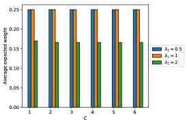
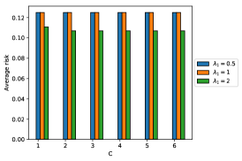
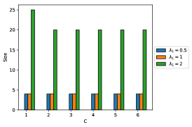
($\alpha$)	($\beta$)	($\gamma$)
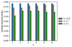
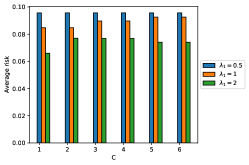
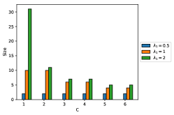
($\delta$)	($\epsilon$)	($\sigma\tau$)
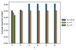
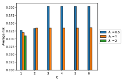
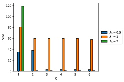
($\zeta$)	($\eta$)	($\theta$)
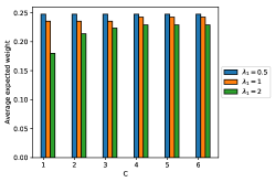
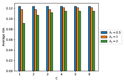
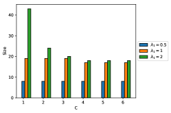
($\iota$)	($\iota\alpha$)	($\iota\beta$)
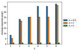
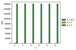
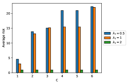
($\iota\gamma$)	($\iota\delta$)	($\iota\epsilon$)

Figure 8: Effect of $C$, $(\lambda_{1},\lambda_{2})$ on risk averse DSD. For details, see text.

References

- [1] Max-cut with negative weight edges by Peter Shor https://cstheory.stackexchange.com/questions/2312/max-cut-with-negative-weight-edges.
- [2] Y. Asahiro, K. Iwama, H. Tamaki, and T. Tokuyama. Greedily finding a dense subgraph. J. Algorithms, 34(2), 2000.
- [3] S. Asthana, O. D. King, F. D. Gibbons, and F. P. Roth. Predicting protein complex membership using probabilistic network reliability. Genome research, 14(6):1170–1175, 2004.
- [4] P. Boldi, F. Bonchi, A. Gionis, and T. Tassa. Injecting uncertainty in graphs for identity obfuscation. Proceedings of the VLDB Endowment, 5(11):1376–1387, 2012.
- [5] B. Bollobás, S. Janson, and O. Riordan. The phase transition in inhomogeneous random graphs. Random Structures & Algorithms, 31(1):3–122, 2007.
- [6] F. Bonchi, F. Gullo, A. Kaltenbrunner, and Y. Volkovich. Core decomposition of uncertain graphs. In Proc. of the 20th ACM SIGKDD conference, pages 1316–1325. ACM, 2014.
- [7] J. Cadena, A. K. Vullikanti, and C. C. Aggarwal. On dense subgraphs in signed network streams. In 2016 IEEE 16th International Conference on Data Mining (ICDM), pages 51–60. IEEE, 2016.
- [8] M. Charikar. Greedy approximation algorithms for finding dense components in a graph. In APPROX, 2000.
- [9] M. Charikar, Y. Naamad, and J. Wu. On finding dense common subgraphs. arXiv preprint arXiv:1802.06361, 2018.
- [10] T. Chen and C. E. Tsourakakis. Tmdb uncertain graph. https://drive.google.com/open?id=1C69MndtfSoUflPkeBa0mbiC9FZD6xbpN.
- [11] W. Chen, T. Lin, Z. Tan, M. Zhao, and X. Zhou. Robust influence maximization. In Proceedings of the 22nd ACM SIGKDD International Conference on Knowledge Discovery and Data Mining, pages 795–804. ACM, 2016.
- [12] S. R. Collins, P. Kemmeren, X.-C. Zhao, J. F. Greenblatt, F. Spencer, F. C. Holstege, J. S. Weissman, and N. J. Krogan. Toward a comprehensive atlas of the physical interactome of saccharomyces cerevisiae. Molecular & Cellular Proteomics, 6(3):439–450, 2007.
- [13] N. N. Dalvi and D. Suciu. Efficient query evaluation on probabilistic databases. VLDB J., 16(4):523–544, 2007.
- [14] E. Galimberti, F. Bonchi, and F. Gullo. Core decomposition and densest subgraph in multilayer networks. In Proceedings of the 2017 ACM on Conference on Information and Knowledge Management, pages 1807–1816. ACM, 2017.
- [15] E. Galimberti, F. Bonchi, F. Gullo, and T. Lanciano. Core decomposition in multilayer networks: Theory, algorithms, and applications. arXiv preprint arXiv:1812.08712, 2018.
- [16] G. Gallo, M. D. Grigoriadis, and R. E. Tarjan. A fast parametric maximum flow algorithm and applications. Journal of Computing, 18(1), 1989.
- [17] A.-C. Gavin, P. Aloy, P. Grandi, R. Krause, M. Boesche, M. Marzioch, C. Rau, L. J. Jensen, S. Bastuck, B. Dümpelfeld, et al. Proteome survey reveals modularity of the yeast cell machinery. Nature, 440(7084):631, 2006.
- [18] A. Gionis and C. E. Tsourakakis. Dense subgraph discovery: Kdd 2015 tutorial. In Proceedings of the 21th ACM SIGKDD International Conference on Knowledge Discovery and Data Mining, pages 2313–2314. ACM, 2015.
- [19] A. V. Goldberg. Finding a maximum density subgraph. Technical report, University of California at Berkeley, 1984.
- [20] D. Gunopulos and G. Das. Time series similarity measures and time series indexing. In ACM Sigmod Record, 2001.
- [21] J. Hastad. Clique is hard to approximate within . Acta Mathematica, 182(1), 1999.
- [22] X. He and D. Kempe. Robust influence maximization. In Proceedings of the 22Nd ACM SIGKDD International Conference on Knowledge Discovery and Data Mining, KDD ’16, pages 885–894, New York, NY, USA, 2016. ACM.
- [23] X. Huang, W. Lu, and L. V. Lakshmanan. Truss decomposition of probabilistic graphs: Semantics and algorithms. In Proceedings of SIGMOD 2016, pages 77–90, 2016.
- [24] R. Jin, L. Liu, and C. C. Aggarwal. Discovering highly reliable subgraphs in uncertain graphs. In Proceedings of KDD 2011, pages 992–1000, 2011.
- [25] R. M. Karp. Reducibility among combinatorial problems. In R. Miller and J. Thatcher, editors, Complexity of Computer Computations. 1972.
- [26] D. Kempe, J. Kleinberg, and É. Tardos. Maximizing the spread of influence through a social network. In Proceedings of KDD 2003, pages 137–146. ACM, 2003.
- [27] A. Khan and L. Chen. On uncertain graphs modeling and queries. Proceedings of the VLDB Endowment, 8(12):2042–2043, 2015.
- [28] S. Khuller and B. Saha. On finding dense subgraphs. In 36th International Colloquium on Automata, Languages and Programming (ICALP), 2009.
- [29] G. Kollios, M. Potamias, and E. Terzi. Clustering large probabilistic graphs. IEEE Transactions on Knowledge and Data Engineering, 25(2):325–336, 2013.
- [30] N. J. Krogan, G. Cagney, H. Yu, G. Zhong, X. Guo, A. Ignatchenko, J. Li, S. Pu, N. Datta, A. P. Tikuisis, et al. Global landscape of protein complexes in the yeast saccharomyces cerevisiae. Nature, 440(7084):637, 2006.
- [31] P. lab. http://www.paccanarolab.org/static_content/clusterone/cl1_datasets.zip.
- [32] E. L. Lawler. Combinatorial optimization: networks and matroids. Courier Corporation, 2001.
- [33] L. Liu, R. Jin, C. Aggarwal, and Y. Shen. Reliable clustering on uncertain graphs. In Proceedings of ICDM 2012, pages 459–468. IEEE, 2012.
- [34] M. Mitzenmacher, J. Pachocki, R. Peng, C. Tsourakakis, and S. C. Xu. Scalable large near-clique detection in large-scale networks via sampling. In Proceedings of the 21th ACM SIGKDD International Conference on Knowledge Discovery and Data Mining, pages 815–824. ACM, 2015.
- [35] A. Miyauchi and A. Takeda. Robust densest subgraph discovery. In 2018 IEEE International Conference on Data Mining (ICDM), pages 1188–1193. IEEE, 2018.
- [36] W. E. Moustafa, A. Kimmig, A. Deshpande, and L. Getoor. Subgraph pattern matching over uncertain graphs with identity linkage uncertainty. In Proceedings of ICDE 2014, pages 904–915. IEEE, 2014.
- [37] P. Parchas, F. Gullo, D. Papadias, and F. Bonchi. The pursuit of a good possible world: extracting representative instances of uncertain graphs. In Proceedings SIGMOD 2014, pages 967–978, 2014.
- [38] M. Potamias, F. Bonchi, A. Gionis, and G. Kollios. K-nearest neighbors in uncertain graphs. Proceedings of the VLDB Endowment, 3(1-2):997–1008, 2010.
- [39] P. Pratikakis. twawler: A lightweight twitter crawler. arXiv preprint arXiv:1804.07748, 2018.
- [40] R. Ravi and M. X. Goemans. The constrained minimum spanning tree problem. In Scandinavian Workshop on Algorithm Theory, pages 66–75. Springer, 1996.
- [41] A. E. Roth, T. Sönmez, and M. U. Ünver. Kidney exchange. The Quarterly Journal of Economics, 119(2):457–488, 2004.
- [42] K. Semertzidis, E. Pitoura, E. Terzi, and P. Tsaparas. Best friends forever (bff): Finding lasting dense subgraphs. arXiv preprint arXiv:1612.05440, 2016.
- [43] J. Serra and J. L. Arcos. An empirical evaluation of similarity measures for time series classification. Knowledge-Based Systems, 67:305–314, 2014.
- [44] C. Tsourakakis. Streaming graph partitioning in the planted partition model. In Proceedings of the 2015 ACM on Conference on Online Social Networks, pages 27–35. ACM, 2015.
- [45] C. Tsourakakis, F. Bonchi, A. Gionis, F. Gullo, and M. Tsiarli. Denser than the densest subgraph: extracting optimal quasi-cliques with quality guarantees. In Proceedings of the 19th ACM SIGKDD international conference on Knowledge discovery and data mining, pages 104–112. ACM, 2013.
- [46] C. Tsourakakis, C. Gkantsidis, B. Radunovic, and M. Vojnovic. Fennel: Streaming graph partitioning for massive scale graphs. In Proceedings of the 7th ACM international conference on Web search and data mining, pages 333–342. ACM, 2014.
- [47] C. E. Tsourakakis. The k-clique densest subgraph problem. 24th International World Wide Web Conference (WWW), 2015.
- [48] C. E. Tsourakakis, S. Sekar, J. Lam, and L. Yang. Risk-averse matchings over uncertain graph databases. arXiv preprint arXiv:1801.03190, 2018.
- [49] B. Wilder, A. Yadav, N. Immorlica, E. Rice, and M. Tambe. Uncharted but not uninfluenced: Influence maximization with an uncertain network. In Proceedings of the 16th Conference on Autonomous Agents and MultiAgent Systems, pages 1305–1313. International Foundation for Autonomous Agents and Multiagent Systems, 2017.
- [50] Y. Yang, N. Chawla, Y. Sun, and J. Hani. Predicting links in multi-relational and heterogeneous networks. In 2012 IEEE 12th international conference on data mining, pages 755–764. IEEE, 2012.
- [51] Z. Zou. Polynomial-time algorithm for finding densest subgraphs in uncertain graphs. In Proceedings of MLG Workshop, 2013.