AN ALTERNATIVE VIEW ON THE BATEMAN-LUKE
VARIATIONAL PRINCIPLE
Hamid Alemi Ardakani
Department of Mathematics, University of Exeter, Penryn Campus, Cornwall TR10 9FE, UK

Abstract. A new derivation of the Bernoulli equation for water waves in three-dimensional rotating and translating coordinate systems is given. An alternative view on the Bateman-Luke variational principle is presented. The variational principle recovers the boundary value problem governing the motion of potential water waves in a container undergoing prescribed rigid-body motion in three dimensions. A mathematical theory is presented for the problem of three-dimensional interactions between potential surface waves and a floating structure with interior potential fluid sloshing. The complete set of equations of motion for the exterior gravity-driven water waves, and the exact nonlinear hydrodynamic equations of motion for the linear momentum and angular momentum of the floating structure containing fluid, are derived from a second variational principle. The two-dimensional form of the 3–D variational principles and their corresponding partial differential equations are presented.

1 Introduction

The Bateman-Luke variational principle (Bateman 1932; Luke 1967) for the problem of fluid sloshing in a container undergoing prescribed rigid-body motion in three dimensions is given by Lukovsky (1990), Lukovsky (2015), Faltinsen & Timokha (2009), Timokha (2016) and Faltinsen et al. (2000) as

$$\begin{array}[]{rcl}&&\displaystyle\delta\mathcal{L}\left(\Phi,\xi\right)=\delta\int_{t_{1}}^{t_{2}}\int_{\mathcal{Q}\left(t\right)}-\rho\left(\frac{\partial\Phi}{\partial t}+\mbox{$\frac{1}{2}$}\nabla\Phi\cdot\nabla\Phi-\nabla\Phi\cdot\left(\bm{v}_{0}+\bm{\omega}\times\bm{r}\right)+U\right){\rm d}\mathcal{Q}\,{\rm d}t=0\,,\end{array}$$ (1.1)

where $\mathcal{Q}\left(t\right)$ is the fluid volume bounded by the free surface $\Sigma\left(t\right)$ and the wetted tank surface $S\left(t\right)$, $\Phi\left(x,y,z,t\right)$ is the velocity potential of the interior irrotational flow in a moving coordinate system $Oxyz$ fixed with respect to the rigid tank, the origin of the moving coordinate system $Oxyz$ is in the unperturbed free surface and moves with the velocity $\bm{v}_{0}$ relative to a fixed coordinate system $O^{\prime}x^{\prime}y^{\prime}z^{\prime}$, $\xi\left(x,y,t\right)$ is the free surface height relative to the moving frame $O$, $\bm{\omega}$ is the angular velocity of the tank relative to the fixed coordinate system $O^{\prime}x^{\prime}y^{\prime}z^{\prime}$, and $U\left(x,y,z,t\right)$ is the gravity field potential defined as

$$U\left(x,y,z,t\right)=-\bm{g}\cdot\bm{r}^{\prime}\quad\mbox{with}\quad\bm{r}^{\prime}=\bm{r}_{0}^{\prime}+\bm{r}\,,$$ (1.2)

where $\bm{r}^{\prime}$ is the radius-vector of a point of the fluid-body system with respect to the fixed frame $O^{\prime}$, $\bm{r}_{0}^{\prime}$ is the radius-vector of the origin of the moving frame $O$ with respect to the origin of the fixed frame $O^{\prime}$, $\bm{r}$ is the radius-vector with respect to $O$ and $\bm{g}$ is the gravity acceleration vector. Taking the variations $\delta\Phi$ and $\delta\xi$ in the variational principle (1.1) subject to the restrictions $\delta\Phi=0$ at the end points of the time interval, $t_{1}$ and $t_{2}$, gives the following boundary value problem (Faltinsen et al. 2000)

$$\left.\begin{array}[]{rcl}&&\displaystyle\Delta\,\Phi:=\Phi_{xx}+\Phi_{yy}+\Phi_{zz}=0\quad\mbox{in}\quad\mathcal{Q}\left(t\right)\,,\\[8.53581pt] &&\displaystyle\frac{\partial\Phi}{\partial\bm{n}}=\bm{v}_{0}\cdot\bm{n}+\bm{\omega}\cdot\left(\bm{r}\times\bm{n}\right)\quad\mbox{on}\quad S\left(t\right)\,,\\[8.53581pt] &&\displaystyle\frac{\partial\Phi}{\partial\bm{n}}=\bm{v}_{0}\cdot\bm{n}+\bm{\omega}\cdot\left(\bm{r}\times\bm{n}\right)+\frac{\xi_{t}}{\sqrt{1+\xi_{x}^{2}+\xi_{y}^{2}}}\quad\mbox{on}\quad\Sigma\left(t\right)\,,\\[8.53581pt] &&\displaystyle\frac{\partial\Phi}{\partial t}+\mbox{$\frac{1}{2}$}\nabla\Phi\cdot\nabla\Phi-\nabla\Phi\cdot\left(\bm{v}_{0}+\bm{\omega}\times\bm{r}\right)+U=0\quad\mbox{on}\quad\Sigma\left(t\right)\,,\end{array}\right\}$$ (1.3)

where $\bm{n}$ is the outer normal to the boundary of $\mathcal{Q}\left(t\right)$. The second equation in (1.3) gives the rigid-wall boundary condition, the third equation in (1.3) is the kinematic free surface boundary condition, and the last equation in (1.3) is the dynamic free surface boundary condition deduced from Bernoulli’s equation. The Bernoulli equation for the hydrodynamic pressure $p$ in $\mathcal{Q}\left(t\right)$ takes the form (Faltinsen et al. 2000; Faltinsen & Timokha 2009)

$$\frac{\partial\Phi}{\partial t}+\frac{p}{\rho}+\mbox{$\frac{1}{2}$}\nabla\Phi\cdot\nabla\Phi-\nabla\Phi\cdot\left(\bm{v}_{0}+\bm{\omega}\times\bm{r}\right)+U=0\,,$$ (1.4)

where $\rho$ is the density of the fluid and $\partial\Phi/\partial t$ is calculated in the moving coordinate system, i.e. for a point rigidly connected with the system $Oxyz$.

It is stated in the literature that Bernoulli’s equation which is a result of integrating the Euler equations relative to the fixed coordinate system, i.e. $O^{\prime}x^{\prime}y^{\prime}z^{\prime}$, is only valid in an inertial system and hence cannot directly be applied to an accelerated coordinate system, i.e. $Oxyz$. Hence, the Bernoulli equation (1.4), in the moving coordinate system, is obtained by transforming the Bernoulli equation from the fixed coordinate system $O^{\prime}$ to the moving coordinate system $O$, by relating $\partial\Phi/\partial t$ between the inertial and moving coordinate systems.

Our main goal in the first part of the current paper, §2 and §3, is to present a new derivation of the Bernoulli equation (1.4) by integrating the Euler equations relative to the rotating and translating coordinate system attached to the moving container, using the vorticity equation. The proposed Bernoulli equation is then used to present an alternative view on the Bateman-Luke variational principle (1.1) and the boundary value problem (1.3) for water waves in moving coordinate systems.

Variational principles for the motion of a rigid body dynamically coupled to its interior fluid motion are given by Moiseyev & Rumyantsev (1968) and Lukovsky (2015) (and references therein). In the work by Lukovsky (2015), the Bateman-Luke variational principle is used to develop a mathematical theory for interactions between potential surface waves and a floating rigid body containing cavities filled partially with a homogeneous incompressible ideal liquid. Alemi Ardakani (2019) derived a variational principle for the three-dimensional interactions between gravity-driven potential water waves and a floating rigid body dynamically coupled to its interior inviscid and incompressible fluid sloshing governed by the Euler equations relative to the rotating-translating coordinate system attached to the body. The variational principle gives the complete set of equations of motion for the exterior water waves, the Euler-Poincaré equations for the angular momentum and linear momentum of the rigid-body, and the Euler equations for the motion of the interior fluid of the rigid-body relative to the body coordinate system.

The main goal in the second part of the current paper, §4, is to develop a mathematical theory for three-dimensional (3–D) interactions between potential surface waves and a floating structure dynamically coupled to its interior potential fluid sloshing relative to the rotating and translating coordinate system attached to the moving body. The Bateman-Luke variational principle, presented in §3, recovers the Neumann boundary value problem, in terms of the velocity potential, governing the motion of the interior fluid of the floating rigid-body interacting with the exterior ocean waves. The aim in §4 is to present a second variational principle which recovers the equations of motion for the exterior potential water waves, and gives the exact hydrodynamic equations of motion for the angular momentum and linear momentum of the floating rigid-body dynamically coupled to its interior potential fluid motion. Adapting the variational principles developed by Alemi Ardakani (2019), the required variational principle takes the form

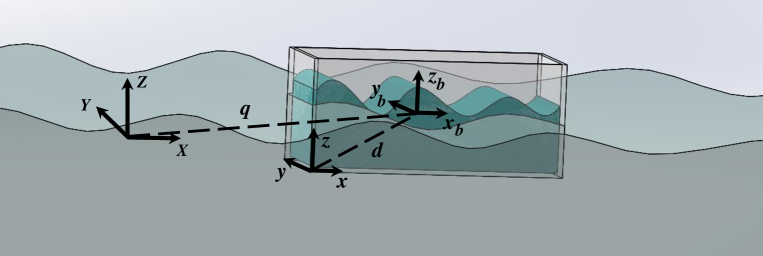
Figure 1: Schematic showing a floating structure containing fluid in hydrodynamic interaction with exterior ocean waves.

$$\delta\mathscr{L}\left(\phi,\eta,\bm{\Omega},\bm{Q},\bm{q},\dot{\bm{q}}\right)=\delta\mathscr{L}_{1}\left(\phi,\eta\right)+\delta\mathscr{L}_{2}\left(\bm{\Omega},\bm{Q},\bm{q},\dot{\bm{q}}\right)=0\,,$$ (1.5)

where

$$\begin{array}[]{rcl}&&\displaystyle\mathscr{L}_{1}\left(\phi,\eta\right)=\displaystyle\int_{t_{1}}^{t_{2}}\int_{V\left(t\right)}-\rho\left(\phi_{t}+\mbox{$\frac{1}{2}$}\nabla\phi\cdot\nabla\phi+gZ\right){\rm d}V\,{\rm d}t\,,\end{array}$$ (1.6)

and

$$\begin{array}[]{rcl}&&\displaystyle\mathscr{L}_{2}\left(\bm{\Omega},\bm{Q},\bm{q},\dot{\bm{q}}\right)=\int^{t_{2}}_{t_{1}}\left(\int_{\mathcal{Q}}\left(\mbox{$\frac{1}{2}$}\left\Arrowvert\bm{u}\right\Arrowvert^{2}+\bm{u}\cdot\left(\bm{\Omega}\times\left(\bm{x}+\bm{d}\right)+\bm{Q}^{T}\dot{\bm{q}}\right)+\bm{Q}^{T}\dot{\bm{q}}\cdot\left(\bm{\Omega}\times\left(\bm{x}+\bm{d}\right)\right)\right.\right.\\[8.53581pt] &&\displaystyle\left.\left.\hskip 142.26378pt+\mbox{$\frac{1}{2}$}\left\Arrowvert\dot{\bm{q}}\right\Arrowvert^{2}-g\left(\bm{Q}\left(\bm{x}+\bm{d}\right)+\bm{q}\right)\cdot\bm{k}\right)\rho\,{\rm d}\bm{x}+\mbox{$\frac{1}{2}$}\bm{\Omega}\cdot\bm{I}_{f}\bm{\Omega}\right.\\[8.53581pt] &&\displaystyle\left.\hskip 85.35826pt+\mbox{$\frac{1}{2}$}m_{v}\left\Arrowvert\dot{\bm{q}}\right\Arrowvert^{2}+\left(\bm{\Omega}\times m_{v}\overline{\bm{x}}_{v}\right)\cdot\bm{Q}^{T}\dot{\bm{q}}+\mbox{$\frac{1}{2}$}\bm{\Omega}\cdot\bm{I}_{v}\bm{\Omega}-m_{v}g\left(\bm{Q}\overline{\bm{x}}_{v}+\bm{q}\right)\cdot\bm{k}\right){\rm d}t\,,\end{array}$$ (1.7)

where in the derivation of the Lagrangian functional (1.5), three frames of reference are used. The spatial frame, which is fixed in space, has coordinates denoted by $\bm{X}=\left(X,Y,Z\right)$. The first body frame, which is placed at the centre of rotation of the moving body and used for the analysis of the rigid body motion, has coordinates denoted by $\bm{x}_{b}=\left(x_{b},y_{b},z_{b}\right)$. The second body frame, which is attached to the moving body and used for the analysis of the fluid motion inside the tank, has coordinates denoted by $\bm{x}=\left(x,y,z\right)$. The distance between the origin of the body frame $\bm{x}$ to the point of rotation, i.e. the origin of the body frame $\bm{x}_{b}$, is denoted by $\bm{d}=\left(d_{1},d_{2},d_{3}\right)$ which is a constant vector. So the position of a fluid particle relative to the body frame $\bm{x}_{b}$ is $\bm{x}_{b}=\bm{x}+\bm{d}$. The fluid-tank system has a uniform translation $\bm{q}\left(t\right)=\left(q_{1}(t),q_{2}(t),q_{3}(t)\right)$ relative to the spatial frame $\bm{X}$, which is the vector from the origin of the spatial frame $\bm{X}$ to the origin of the body frame $\bm{x}_{b}$. In (1.5), $\bm{u}\left(x,y,z,t\right)$ is the Eulerian velocity of a fluid particle in the body frame $\bm{x}$, $\mathcal{Q}$ is the volume of the fluid inside the tank, $\bm{k}$ is the unit vector in the $Z$ direction, $g$ is the acceleration due to gravity, $\rho$ is the water density which is assumed to be the same for the interior and exterior fluids, $\bm{Q}\left(t\right)\in\mbox{SO}\left(3\right)$ is a proper rotation in $\mathbb{R}^{3}$, i.e. $\bm{Q}^{T}\bm{Q}=\bm{I}$ and ${\rm det}\left(\bm{Q}\right)=1$, the body angular velocity is a time-dependent vector $\bm{\Omega}\left(t\right)=\left(\Omega_{1}\left(t\right),\Omega_{2}\left(t\right),\Omega_{3}\left(t\right)\right)$ relative to the body coordinate system $\bm{x}_{b}$ with entries determined from the rotation tensor $\bm{Q}\left(t\right)$ by $\widehat{\bm{\Omega}}=\bm{Q}^{T}\dot{\bm{Q}}$ such that the skew-symmetric matrix $\widehat{\bm{\Omega}}$ satisfies $\widehat{\bm{\Omega}}\bm{\mathrm{r}}=\bm{\Omega}\times\bm{\mathrm{r}}$ for any $\bm{\mathrm{r}}\in\mathbb{R}^{3}$ (see Alemi Ardakani (2019) for more details), $\bm{I}_{f}$ which is defined as

$$\bm{I}_{f}=\int_{\mathcal{Q}}\left(\left\Arrowvert\bm{x}+\bm{d}\right\Arrowvert^{2}\bm{I}-\left(\bm{x}+\bm{d}\right)\otimes\left(\bm{x}+\bm{d}\right)\right)\rho\,{\rm d}\bm{x}\,,$$ (1.8)

is the mass moment of inertia of the interior fluid relative to the point of rotation, i.e. the origin of the body frame $\bm{x}_{b}$, $\otimes$ denotes the tensor product, $\bm{I}$ is the $3\times 3$ identity matrix, $\bm{I}_{v}$ is the mass moment of inertia of the dry floating body relative to the point of rotation, $m_{v}$ is the mass of the dry body, $\overline{\bm{x}}_{v}=\left(\overline{x}_{v},\overline{y}_{v},\overline{z}_{v}\right)$ is the centre of mass of the dry body relative to the body frame $\bm{x}_{b}$, $\phi\left(X,Y,Z,t\right)$ and $\eta\left(X,Y,t\right)$ are respectively the velocity potential and the free surface elevation of the exterior irrotational water waves, and $V\left(t\right)$ is the transient domain of the exterior fluid. The configuration of the fluid in a rotating and translating floating structure in hydrodynamic interaction with exterior water waves is schematically shown in Figure 1.

The paper starts with the derivation of the Bernoulli equation and the Neumann boundary value problem for an inviscid and incompressible fluid sloshing in a container undergoing prescribed rigid-body motion in three dimensions in §2. In §3, the Bateman-Luke variational principle is revisited for the problem of fluid sloshing in rotating and translating coordinates. In §4, a variational principle is given for 3–D interactions between ocean waves and a floating structure containing fluid. The paper ends with concluding remarks in §5. In Appendix A, the proposed 3–D variational principles of §3 and §4 are reduced for the problem of two-dimensional (2–D) interactions between potential surface waves and a floating structure dynamically coupled to its interior potential fluid sloshing. The 2–D wave–body–slosh variational principles are given in Alemi Ardakani (2017). However, the presented variational principles of Alemi Ardakani (2017) are modified in Appendix A.

2 Derivation of the Bernoulli equation for the pressure field in rotating and translating coordinate systems

The configuration of the fluid in a rotating-translating rectangular vessel is schematically shown in Figure 1. The vessel is a rigid body, which is free to rotate or translate in $\mathbb{R}^{3}$. The vessel is partially filled with an inviscid and incompressible fluid. The position of a fluid particle in the body frame $\bm{x}$ is related to a point in the spatial frame $\bm{X}$ by

$$\bm{X}=\bm{Q}\left(\bm{x}+\bm{d}\right)+\bm{q}\,,$$ (2.1)

and the Eulerian velocity of a fluid particle $\bm{u}\left(\bm{x},t\right)$ in the body frame $\bm{x}$ is related to the its velocity $\bm{U}\left(\bm{X},t\right)$ in the spatial frame $\bm{X}$ by (Alemi Ardakani & Bridges 2011; Alemi Ardakani 2019)

$$\bm{U}=\bm{Q}\left(\bm{u}+\bm{\Omega}\times\left(\bm{x}+\bm{d}\right)+\bm{Q}^{T}\dot{\bm{q}}\right)\,,$$ (2.2)

where the rotation tensor $\bm{Q}$ and the body angular velocity $\bm{\Omega}$ are defined in §1. It is shown in Alemi Ardakani & Bridges (2011) that the Euler equations for the motion of an inviscid and incompressible fluid relative to the body coordinate system $\bm{x}$ takes the form

$$\frac{D\bm{u}}{Dt}+\frac{1}{\rho}\nabla p=-2\bm{\Omega}\times\bm{u}-\dot{\bm{\Omega}}\times\left(\bm{x}+\bm{d}\right)-\bm{\Omega}\times\left(\bm{\Omega}\times\left(\bm{x}+\bm{d}\right)\right)-\bm{Q}^{T}\bm{g}-\bm{Q}^{T}\ddot{\bm{q}}\,,$$ (2.3)

where $\bm{u}=\left(u,v,w\right)$, $D\bm{u}/Dt=\bm{u}_{t}+\left(\bm{u}\cdot\nabla\right)\bm{u}$ and $\bm{g}=g\bm{k}$. The term $\bm{Q}^{T}\bm{g}$ rotates the usual gravity vector so that its direction is viewed properly in the body frame $\bm{x}_{b}$. The same is true for the translational acceleration $\ddot{\bm{q}}$.

The fluid occupies the region $\mathcal{Q}\left(t\right)$ in the vessel which is bounded by the free surface $\Sigma\left(t\right)$ and the wetted tank surface $S\left(t\right)$,

$$0\leq x\leq L_{1}\,,\quad 0\leq y\leq L_{2}\,,\quad 0\leq z\leq h\left(x,y,t\right)\,,$$ (2.4)

where the lengths $L_{1}$ and $L_{2}$ are given positive constants, and $z=h\left(x,y,t\right)$ is the position of the free surface inside the vessel, relative to the body frame $\bm{x}$.

Conservation of mass relative to the body frame $\bm{x}$ takes the form

$$\nabla\cdot\bm{u}=u_{x}+v_{y}+w_{z}=0\,.$$ (2.5)

The boundary conditions are

$$\left.\begin{array}[]{rcl}u&=&0\quad\mbox{at}\quad x=0\quad\mbox{and}\quad x=L_{1}\,,\\[5.69054pt] v&=&0\quad\mbox{at}\quad y=0\quad\mbox{and}\quad y=L_{2}\,,\\[5.69054pt] w&=&0\quad\mbox{at}\quad z=0\,,\end{array}\right\}$$ (2.6)

which are the no-flow boundary conditions on the rigid walls, and at the free surface, the kinematic and dynamic boundary conditions are respectively

$$w=h_{t}+uh_{x}+vh_{y}\quad\mbox{and}\quad p=0\quad\mbox{at}\quad z=h\left(x,y,t\right)\,,$$ (2.7)

where the surface tension is neglected in the boundary condition for the pressure $p$.

The vorticity vector is defined by

$$\bm{\mathcal{V}}:=\nabla\times\bm{u}\,.$$ (2.8)

Differentiating this equations gives

$$\frac{D\bm{\mathcal{V}}}{Dt}=\bm{\mathcal{V}}\cdot\nabla\bm{u}+\nabla\times\left(\frac{D\bm{u}}{Dt}\right)\,.$$ (2.9)

Taking the curl of the Euler equations (2.3) gives

$$\nabla\times\left(\frac{D\bm{u}}{Dt}\right)=2\bm{\Omega}\cdot\nabla\bm{u}-2\dot{\bm{\Omega}}\,.$$ (2.10)

Substitution of (2.10) into (2.9) gives the vorticity equation

$$\frac{D\bm{\mathcal{V}}}{Dt}=\left(2\bm{\Omega}+\bm{\mathcal{V}}\right)\cdot\nabla\bm{u}-2\dot{\bm{\Omega}}\,.$$ (2.11)

Now, if we set

$$\bm{\mathcal{V}}=-2\bm{\Omega}\,,$$ (2.12)

then

$$\frac{D\bm{\mathcal{V}}}{Dt}=-2\dot{\bm{\Omega}}\,,$$ (2.13)

and the vorticity equation (2.11) is satisfied. Equation (2.12) will be important in the derivation of Bernoulli’s equation in rotating and translating coordinate systems.

Using equation (2.12), the vector identity

$$\frac{D\bm{u}}{Dt}=\frac{\partial\bm{u}}{\partial t}+\nabla\left(\mbox{$\frac{1}{2}$}\bm{u}\cdot\bm{u}\right)-\bm{u}\times\left(\nabla\times\bm{u}\right)\,,$$ (2.14)

takes the form

$$\frac{D\bm{u}}{Dt}=\frac{\partial\bm{u}}{\partial t}+\nabla\left(\mbox{$\frac{1}{2}$}\bm{u}\cdot\bm{u}\right)-2\bm{\Omega}\times\bm{u}\,.$$ (2.15)

Using the vector identity (2.15) the Euler equations (2.3) reduces to

$$\frac{\partial\bm{u}}{\partial t}+\nabla\left(\mbox{$\frac{1}{2}$}\bm{u}\cdot\bm{u}\right)+\frac{1}{\rho}\nabla p+\dot{\bm{\Omega}}\times\left(\bm{x}+\bm{d}\right)+\bm{\Omega}\times\left(\bm{\Omega}\times\left(\bm{x}+\bm{d}\right)\right)+\bm{Q}^{T}\bm{g}+\bm{Q}^{T}\ddot{\bm{q}}=\bm{0}\,.$$ (2.16)

Now, if we introduce a velocity potential $\Phi\left(x,y,z,t\right)$ such that

$$\bm{u}\left(\bm{x},t\right)=\nabla\Phi\left(\bm{x},t\right)-\bm{\Omega}\times\left(\bm{x}+\bm{d}\right)-\bm{Q}^{T}\dot{\bm{q}}\,,$$ (2.17)

then the velocity field in (2.17) satisfies the vorticity equation. Noting that (Marsden & Ratiu 1999; Holm, Schmah & Stoica 2009)

$$\frac{d}{dt}\left(\bm{Q}^{-1}\right)=-\bm{Q}^{-1}\dot{\bm{Q}}\bm{Q}^{-1}$$ (2.18)

then

$$\frac{\partial\bm{u}}{\partial t}=\nabla\Phi_{t}-\dot{\bm{\Omega}}\times\left(\bm{x}+\bm{d}\right)+\bm{\Omega}\times\bm{Q}^{T}\dot{\bm{q}}-\bm{Q}^{T}\ddot{\bm{q}}\,.$$ (2.19)

Substitution of (2.17) and (2.19) into the Euler equations (2.16) gives

$$\left.\begin{array}[]{rcl}&&\displaystyle\nabla\Phi_{t}+\bm{\Omega}\times\left(\bm{\Omega}\times\left(\bm{x}+\bm{d}\right)+\bm{Q}^{T}\dot{\bm{q}}\right)+\frac{1}{\rho}\nabla p+\bm{Q}^{T}\bm{g}\\[5.69054pt] &&\displaystyle+\nabla\left[\mbox{$\frac{1}{2}$}\nabla\Phi\cdot\nabla\Phi-\nabla\Phi\cdot\left(\bm{\Omega}\times\left(\bm{x}+\bm{d}\right)+\bm{Q}^{T}\dot{\bm{q}}\right)\right.\\[5.69054pt] &&\displaystyle\left.\hskip 19.91692pt+\mbox{$\frac{1}{2}$}\bm{\Omega}\times\left(\bm{x}+\bm{d}\right)\cdot\bm{\Omega}\times\left(\bm{x}+\bm{d}\right)+\bm{\Omega}\times\left(\bm{x}+\bm{d}\right)\cdot\bm{Q}^{T}\dot{\bm{q}}\right]=\bm{0}\,.\end{array}\right\}$$ (2.20)

But

$$\nabla\left(\bm{\Omega}\times\left(\bm{x}+\bm{d}\right)\cdot\bm{Q}^{T}\dot{\bm{q}}\right)=-\bm{\Omega}\times\bm{Q}^{T}\dot{\bm{q}}\,,$$ (2.21)

and

$$\nabla\left(\mbox{$\frac{1}{2}$}\bm{\Omega}\times\left(\bm{x}+\bm{d}\right)\cdot\bm{\Omega}\times\left(\bm{x}+\bm{d}\right)\right)=-\bm{\Omega}\times\left(\bm{\Omega}\times\left(\bm{x}+\bm{d}\right)\right)\,,$$ (2.22)

and so equation (2.20) simplifies to

$$\nabla\left(\Phi_{t}+\frac{p}{\rho}+\mbox{$\frac{1}{2}$}\nabla\Phi\cdot\nabla\Phi-\nabla\Phi\cdot\left(\bm{\Omega}\times\left(\bm{x}+\bm{d}\right)+\bm{Q}^{T}\dot{\bm{q}}\right)+\bm{Q}^{T}\bm{g}\cdot\left(\bm{x}+\bm{d}\right)\right)=\bm{0}\,,$$ (2.23)

or

$$\Phi_{t}+\frac{p}{\rho}+\mbox{$\frac{1}{2}$}\nabla\Phi\cdot\nabla\Phi-\nabla\Phi\cdot\left(\bm{\Omega}\times\left(\bm{x}+\bm{d}\right)+\bm{Q}^{T}\dot{\bm{q}}\right)+\bm{Q}^{T}\bm{g}\cdot\left(\bm{x}+\bm{d}\right)=Be\left(t\right)\,,$$ (2.24)

where $Be\left(t\right)$ is the Bernoulli function which can be absorbed into $\Phi\left(\bm{x},t\right)$. Therefore, Bernoulli’s equation for the pressure field $p$ in $\mathcal{Q}\left(t\right)$ takes the form

$$\Phi_{t}+\frac{p}{\rho}+\mbox{$\frac{1}{2}$}\nabla\Phi\cdot\nabla\Phi-\nabla\Phi\cdot\left(\bm{\Omega}\times\left(\bm{x}+\bm{d}\right)+\bm{Q}^{T}\dot{\bm{q}}\right)+\bm{Q}^{T}\bm{g}\cdot\left(\bm{x}+\bm{d}\right)=0\,.$$ (2.25)

All terms in the new Bernoulli equation (2.25) are relative to the body frame attached to the rotating and translating rigid body.

In terms of the velocity potential $\Phi\left(x,y,z,t\right)$, the rigid-wall boundary conditions in (2.6) become

$$\begin{array}[]{rcl}&&\displaystyle\nabla\Phi=\bm{\Omega}\times\left(\bm{x}+\bm{d}\right)+\bm{Q}^{T}\dot{\bm{q}}\,\quad\mbox{on}\quad S\left(t\right)\,,\end{array}$$ (2.26)

which can be written in the form

$$\begin{array}[]{rcl}&&\displaystyle\frac{\partial\Phi}{\partial\bm{n}_{b}}=\bm{\Omega}\cdot\left(\left(\bm{x}+\bm{d}\right)\times\bm{n}_{b}\right)+\bm{Q}^{T}\dot{\bm{q}}\cdot\bm{n}_{b}\,\quad\mbox{on}\quad S\left(t\right)\,,\end{array}$$ (2.27)

where $\bm{n}_{b}=\bm{Q}^{-1}\bm{n}$ is outer normal to the boundary of $\mathcal{Q}\left(t\right)$ relative to the body frame $\bm{x}_{b}$. Also in terms of the velocity potential $\Phi\left(x,y,z,t\right)$, the kinematic free surface boundary condition in (2.7) becomes

$$\begin{array}[]{rcl}&&\displaystyle\frac{\partial\Phi}{\partial\bm{n}_{b}}=\bm{\Omega}\cdot\left(\left(\bm{x}+\bm{d}\right)\times\bm{n}_{b}\right)+\bm{Q}^{T}\dot{\bm{q}}\cdot\bm{n}_{b}+\frac{h_{t}}{\sqrt{1+h_{x}^{2}+h_{y}^{2}}}\,\quad\mbox{on}\quad\Sigma\left(t\right)\,.\end{array}$$ (2.28)

From (2.25) it can be concluded that the dynamic free surface boundary condition in (2.7) becomes

$$\Phi_{t}+\mbox{$\frac{1}{2}$}\nabla\Phi\cdot\nabla\Phi-\nabla\Phi\cdot\left(\bm{\Omega}\times\left(\bm{x}+\bm{d}\right)+\bm{Q}^{T}\dot{\bm{q}}\right)+\bm{Q}^{T}\bm{g}\cdot\left(\bm{x}+\bm{d}\right)=0\,\quad\mbox{on}\quad\Sigma\left(t\right)\,.$$ (2.29)

Finally, substitution of the velocity field (2.17) into the continuity equation (2.5) leads to Laplace’s equation for $\Phi\left(x,y,z,t\right)$,

$$\Delta\,\Phi=\Phi_{xx}+\Phi_{yy}+\Phi_{zz}=0\,\quad\mbox{in}\quad\mathcal{Q}\left(t\right)\,.$$ (2.30)

In summary, the proposed derivations in this section lead to mathematically precise definitions for all terms in the Bernoulli equation (2.25) and in the corresponding boundary value problem (2.27), (2.28), (2.29) and (2.30) for water waves in moving coordinate systems.

3 The Bateman-Luke variational principle for fluid sloshing in vessels undergoing prescribed rigid-body motion in three dimensions

Based on the new Bernoulli equation (2.25), the Bateman-Luke variational principle (1.1) is modified to

$$\begin{cases}\displaystyle\delta\mathscr{L}\left(\Phi,h\right)=\delta\int_{t_{1}}^{t_{2}}\int_{\mathcal{Q}\left(t\right)}p\left(\bm{x},t\right)\,{\rm d}\mathcal{Q}\,{\rm d}t\\[8.53581pt] \displaystyle=\delta\int_{t_{1}}^{t_{2}}\int_{\mathcal{Q}\left(t\right)}-\left(\Phi_{t}+\mbox{$\frac{1}{2}$}\nabla\Phi\cdot\nabla\Phi-\nabla\Phi\cdot\left(\bm{\Omega}\times\left(\bm{x}+\bm{d}\right)+\bm{Q}^{T}\dot{\bm{q}}\right)+\bm{Q}^{T}\bm{g}\cdot\left(\bm{x}+\bm{d}\right)\right)\,\rho\,{\rm d}\mathcal{Q}\,{\rm d}t=0\,,\end{cases}$$ (3.1)

subject to the endpoint conditions $\delta\Phi\left(\bm{x},t_{1}\right)=\delta\Phi\left(\bm{x},t_{2}\right)=0$. Note that in (3.1), $\bm{\Omega}$ is the body angular velocity, $\bm{Q}^{T}\dot{\bm{q}}$ is the translational velocity of the moving rigid body relative to the body coordinate system $\bm{x}_{b}$, and $\bm{Q}^{T}\bm{g}$ is relative to the body frame $\bm{x}_{b}$, while in (1.1), $\bm{\omega}$ is the angular velocity of the rigid body relative to the spatial coordinate system, $\bm{v}_{0}$ is the translational velocity of the rigid body relative to the spatial frame, and $U=-\bm{g}\cdot\bm{r}^{\prime}$ is relative to the spatial frame.

According to the usual procedure in the calculus of variations, the variational principle (3.1) becomes

$$\left.\begin{array}[]{rcl}&&\displaystyle\delta\mathscr{L}\left(\Phi,h\right)=\int_{t_{1}}^{t_{2}}\int_{\Sigma\left(t\right)}p\left(x,y,h,t\right)\delta h\ell^{-1}\,{\rm d}S\,{\rm d}t\\[8.53581pt] &&\displaystyle+\int_{t_{1}}^{t_{2}}\int_{\mathcal{Q}\left(t\right)}-\left(\delta\Phi_{t}+\nabla\Phi\cdot\nabla\delta\Phi-\nabla\delta\Phi\cdot\left(\bm{\Omega}\times\left(\bm{x}+\bm{d}\right)+\bm{Q}^{T}\dot{\bm{q}}\right)\right)\,\rho\,{\rm d}\mathcal{Q}\,{\rm d}t=0\,,\end{array}\right\}$$ (3.2)

where $\ell=\sqrt{1+h_{x}^{2}+h_{y}^{2}}$ and

$$\begin{array}[]{rcl}p\left(x,y,h,t\right)&=&\displaystyle-\rho\left(\Phi_{t}+\mbox{$\frac{1}{2}$}\nabla\Phi\cdot\nabla\Phi-\nabla\Phi\cdot\left(\bm{\Omega}\times\left(\bm{x}+\bm{d}\right)+\bm{Q}^{T}\dot{\bm{q}}\right)+\bm{Q}^{T}\bm{g}\cdot\left(\bm{x}+\bm{d}\right)\right)\bigg{|}^{z=h\left(x,y,t\right)}\,.\end{array}$$ (3.3)

But

$$\int_{t_{1}}^{t_{2}}\int_{\mathcal{Q}\left(t\right)}-\delta\Phi_{t}\,\rho\,{\rm d}\mathcal{Q}\,{\rm d}t=\int_{t_{1}}^{t_{2}}\int_{\Sigma\left(t\right)}h_{t}\delta\Phi\ell^{-1}\,\rho\,{\rm d}S\,{\rm d}t\,,$$ (3.4)

noting that $\delta\Phi=0$ at $t=t_{1}$ and $t=t_{2}$. Moreover, using Green’s first identity we obtain

$$\begin{cases}\displaystyle-\int_{t_{1}}^{t_{2}}\int_{\mathcal{Q}\left(t\right)}\nabla\Phi\cdot\nabla\delta\Phi\,\rho\,{\rm d}\mathcal{Q}\,{\rm d}t=\int_{t_{1}}^{t_{2}}\int_{\mathcal{Q}\left(t\right)}\Delta\,\Phi\,\delta\Phi\,\rho\,{\rm d}\mathcal{Q}\,{\rm d}t-\int_{t_{1}}^{t_{2}}\int_{\partial\mathcal{Q}}\nabla\Phi\cdot\bm{n}_{b}\,\delta\Phi\,\rho\,{\rm d}S\,{\rm d}t\\[8.53581pt] \displaystyle=\int_{t_{1}}^{t_{2}}\int_{\mathcal{Q}\left(t\right)}\Delta\,\Phi\,\delta\Phi\,\rho\,{\rm d}\mathcal{Q}\,{\rm d}t-\int_{t_{1}}^{t_{2}}\int_{S\left(t\right)}\nabla\Phi\cdot\bm{n}_{b}\,\delta\Phi\,\rho\,{\rm d}S\,{\rm d}t-\int_{t_{1}}^{t_{2}}\int_{\Sigma\left(t\right)}\nabla\Phi\cdot\bm{n}_{b}\,\delta\Phi\,\rho\,{\rm d}S\,{\rm d}t\,,\end{cases}$$ (3.5)

where $\bm{n}_{b}$ is the unit outward normal vector to the boundary of $\mathcal{Q}\left(t\right)$, and also

$$\left.\begin{array}[]{rcl}&&\displaystyle\int_{t_{1}}^{t_{2}}\int_{\mathcal{Q}\left(t\right)}\nabla\delta\Phi\cdot\left(\bm{\Omega}\times\left(\bm{x}+\bm{d}\right)+\bm{Q}^{T}\dot{\bm{q}}\right)\,\rho\,{\rm d}\mathcal{Q}\,{\rm d}t\\[8.53581pt] &&\displaystyle=\int_{t_{1}}^{t_{2}}\int_{S\left(t\right)}\left(\bm{\Omega}\times\left(\bm{x}+\bm{d}\right)+\bm{Q}^{T}\dot{\bm{q}}\right)\cdot\bm{n}_{b}\,\delta\Phi\,\rho\,{\rm d}S\,{\rm d}t\\[11.38109pt] &&\displaystyle+\int_{t_{1}}^{t_{2}}\int_{\Sigma\left(t\right)}\left(\bm{\Omega}\times\left(\bm{x}+\bm{d}\right)+\bm{Q}^{T}\dot{\bm{q}}\right)\cdot\bm{n}_{b}\,\delta\Phi\,\rho\,{\rm d}S\,{\rm d}t\,.\end{array}\right\}$$ (3.6)

Now, substitution of (3.4), (3.5) and (3.6) into the variational principle (3.2) gives

$$\left.\begin{array}[]{rcl}&&\displaystyle\delta\mathscr{L}\left(\Phi,h\right)=\int_{t_{1}}^{t_{2}}\int_{\Sigma\left(t\right)}p\left(x,y,h,t\right)\delta h\ell^{-1}\,{\rm d}S\,{\rm d}t+\int_{t_{1}}^{t_{2}}\int_{\mathcal{Q}\left(t\right)}\Delta\,\Phi\,\delta\Phi\,\rho\,{\rm d}\mathcal{Q}\,{\rm d}t\\[8.53581pt] &&\displaystyle+\int_{t_{1}}^{t_{2}}\int_{\Sigma\left(t\right)}\left(h_{t}\ell^{-1}+\left(-\nabla\Phi+\bm{\Omega}\times\left(\bm{x}+\bm{d}\right)+\bm{Q}^{T}\dot{\bm{q}}\right)\cdot\bm{n}_{b}\right)\delta\Phi\,\rho\,{\rm d}S\,{\rm d}t\\[8.53581pt] &&\displaystyle+\int_{t_{1}}^{t_{2}}\int_{S\left(t\right)}\left(-\nabla\Phi+\bm{\Omega}\times\left(\bm{x}+\bm{d}\right)+\bm{Q}^{T}\dot{\bm{q}}\right)\cdot\bm{n}_{b}\,\delta\Phi\,\rho\,{\rm d}S\,{\rm d}t=0\,.\end{array}\right\}$$ (3.7)

From (3.7), it can be concluded that invariance of $\mathscr{L}$ with respect to a variation in the free surface height $h$ yields the dynamic free surface boundary condition (2.29). Similarly, the invariance of $\mathscr{L}$ with respect to a variation in the velocity potential $\Phi$ at the free surface $\Sigma\left(t\right)$ yields the kinematic free surface boundary condition (2.28), and the invariance of $\mathscr{L}$ with respect to a variation in the velocity potential $\Phi$ along the wetted surface $S\left(t\right)$ recovers the rigid-wall boundary conditions (2.27). Moreover, the invariance of $\mathscr{L}$ with respect to a variation in the velocity potential $\Phi$ yields the field equation (2.30).

4 A variational principle for 3–D interactions between potential surface waves and a floating structure with interior potential fluid sloshing

The interest in this section is to first present a variational principle for the 3–D rotational and translational motion of a rigid body containing fluid such that the interior fluid satisfies the velocity potential theory developed in §2 and §3, and then extend the variational principle for the problem of interactions between potential water waves and a floating structure dynamically coupled to its interior potential fluid sloshing.

Gerrits & Veldman (2003) and Veldman et al. (2007) studied the problem of coupled liquid-solid dynamics for a liquid-filled spacecraft in three dimensions. They presented the differential equations for the motion of the spacecraft containing fluid, describing conservation of linear momentum and angular momentum. The equation for the conservation of angular momentum of the rigid body takes the form (see equation (6) of Gerrits and Veldman (2003) and the work of Alemi Ardakani (2019) for minor modifications of this equation)

$$m_{v}\overline{\bm{x}}_{v}\times\bm{Q}^{-1}\ddot{\bm{q}}+\bm{I}_{v}\dot{\bm{\Omega}}+\bm{\Omega}\times\bm{I}_{v}\bm{\Omega}=\bm{\mathcal{T}}-m_{v}g\overline{\bm{x}}_{v}\times\bm{\chi}\,,$$ (4.1)

where $m_{v}$ is the mass of the dry body, $\overline{\bm{x}}_{v}$ is the centre of mass of the dry body relative to the body frame $\bm{x}_{b}$, $\bm{I}_{v}$ is the mass moment of inertia of the dry body relative to the point of rotation, i.e. the origin of the body frame $\bm{x}_{b}$, $\bm{Q}^{-1}\ddot{\bm{q}}$ is the linear acceleration of the origin of the moving coordinate frame relative to the body frame $\bm{x}_{b}$, and

$$\bm{\mathcal{T}}=\int_{\mathcal{Q}\left(t\right)}\left(\bm{x}+\bm{d}\right)\times\nabla p\,{\rm d}\bm{x}\,,$$ (4.2)

is the torque that the interior fluid exerts on the boundary of the rigid body via pressure, and

$$\bm{\chi}=\bm{Q}^{-1}\bm{k}\,,$$ (4.3)

where $\bm{k}$ is the unit vector in the $Z$ direction. For our problem in this paper, the interior fluid is inviscid and incompressible and satisfies the velocity potential theory developed in §2 and §3. Now, after substituting for $\nabla p$ for the interior fluid of the rigid body from (2.23) in (4.2), equation (4.1) for the body angular velocity $\bm{\Omega}\left(t\right)$ takes the form

$$\begin{cases}\displaystyle\int_{\mathcal{Q}}-\left(\bm{x}+\bm{d}\right)\times\left[\nabla\Phi_{t}+\nabla\left(\mbox{$\frac{1}{2}$}\nabla\Phi\cdot\nabla\Phi\right)-\nabla\left(\nabla\Phi\cdot\left(\bm{\Omega}\times\left(\bm{x}+\bm{d}\right)+\bm{Q}^{T}\dot{\bm{q}}\right)\right)\right]\rho\,{\rm d}\bm{x}\\[8.53581pt] \displaystyle-mg\overline{\bm{x}}\times\bm{\chi}-m_{v}\overline{\bm{x}}_{v}\times\bm{Q}^{-1}\ddot{\bm{q}}-\bm{I}_{v}\dot{\bm{\Omega}}+\bm{I}_{v}\bm{\Omega}\times\bm{\Omega}=\bm{0}\,,\end{cases}$$ (4.4)

where $m$ is the total mass of the (interior fluid + body) system,

$$m=m_{f}+m_{v}\quad\mbox{with}\quad m_{f}=\int_{\mathcal{Q}}\rho\,{\rm d}\bm{x}\,,$$ (4.5)

where $m_{f}$ is the mass of the interior fluid which is time independent. Note that in $(\ref{Omega-equation})$ $\overline{\bm{x}}$ is the centre of mass of the coupled (interior fluid + body) system relative to the body frame $\bm{x}_{b}$, which is time dependent and satisfies

$$m\overline{\bm{x}}\left(t\right)=m_{f}\overline{\bm{x}}_{f}+m_{v}\overline{\bm{x}}_{v}\,,$$ (4.6)

with

$$m_{f}\overline{\bm{x}}_{f}=\int_{\mathcal{Q}}\left(\bm{x}+\bm{d}\right)\rho\,{\rm d}\bm{x}\,,$$ (4.7)

where $\overline{\bm{x}}_{f}\left(t\right)$ is the centre of mass of the interior fluid relative to the body frame $\bm{x}_{b}$.

Similarly, the equation for the conservation of linear momentum of the rigid body takes the form (see equation (5) of Gerrits and Veldman (2003))

$$m_{v}\bm{Q}^{-1}\ddot{\bm{q}}+\dot{\bm{\Omega}}\times m_{v}\overline{\bm{x}}_{v}+\bm{\Omega}\times\left(\bm{\Omega}\times m_{v}\overline{\bm{x}}_{v}\right)=\bm{\mathcal{F}}-m_{v}g\bm{\chi}\,,$$ (4.8)

where

$$\bm{\mathcal{F}}=\int_{\mathcal{Q}\left(t\right)}\nabla p\,{\rm d}\bm{x}\,,$$ (4.9)

is the force that the interior fluid exerts on the boundary of the rigid body via pressure. Now, after substituting for $\nabla p$ from (2.23) in (4.9), equation (4.8) for the translational motion of the rigid body $\bm{q}\left(t\right)$ takes the form

$$\begin{cases}\displaystyle\int_{\mathcal{Q}}-\left[\nabla\Phi_{t}+\nabla\left(\mbox{$\frac{1}{2}$}\nabla\Phi\cdot\nabla\Phi\right)-\nabla\left(\nabla\Phi\cdot\left(\bm{\Omega}\times\left(\bm{x}+\bm{d}\right)+\bm{Q}^{T}\dot{\bm{q}}\right)\right)\right]\rho\,{\rm d}\bm{x}\\[8.53581pt] \displaystyle-mg\bm{\chi}-m_{v}\bm{Q}^{-1}\ddot{\bm{q}}-\dot{\bm{\Omega}}\times m_{v}\overline{\bm{x}}_{v}-\bm{\Omega}\times\left(\bm{\Omega}\times m_{v}\overline{\bm{x}}_{v}\right)=\bm{0}\,.\end{cases}$$ (4.10)

The Lagrangian action for the motion of a rigid-body dynamically coupled to its interior fluid motion takes the form

$$\mathscr{L}=\int^{t_{2}}_{t_{1}}\left(\mathrm{KE}^{fluid}-\mathrm{PE}^{fluid}+\mathrm{KE}^{body}-\mathrm{PE}^{body}\right){\rm d}t\,,$$ (4.11)

where $\mathrm{KE}^{fluid}$ is the kinetic energy of the fluid, $\mathrm{KE}^{body}$ is the kinetic energy of the rigid body, $\mathrm{PE}^{fluid}$ is the potential energy of the fluid and $\mathrm{PE}^{body}$ is the potential energy of the rigid body. It is shown in Alemi Ardakani (2019) that the action functional (4.11) for a rigid body which contains an inviscid and incompressible fluid and undergoes three dimensional rotational and translational motions takes the form (1.7). The equations of motion for the body angular velocity $\bm{\Omega}\left(t\right)$ and the translational motion $\bm{q}\left(t\right)$ of the rigid body are provided by Hamilton’s variational principle:

$$\delta\mathscr{L}_{2}\left(\bm{\Omega},\bm{Q},\bm{q},\dot{\bm{q}}\right)=0\,,$$ (4.12)

subject to the fixed endpoints $\delta\bm{q}\left(t_{1}\right)=\delta\bm{q}\left(t_{2}\right)=\bm{0}$, and noting that the variations $\delta\bm{Q}$ are taken among paths $\bm{Q}\left(t\right)\in\mbox{SO}\left(3\right)$, $t\in[t_{1},t_{2}]$, with fixed endpoints, so that $\delta\bm{Q}\left(t_{1}\right)=\delta\bm{Q}\left(t_{2}\right)=\bm{0}$. It is proved in Alemi Ardakani (2019) that taking the variations $\delta\bm{\Omega}$, $\delta\bm{Q}$, $\delta\bm{q}$ and $\delta\dot{\bm{q}}$ in the variational principle (4.12), using the Euler-Poincaré framework (Marsden & Ratiu 1999; Holm, Schmah & Stoica 2009), gives the Euler-Poincaré equation for $\bm{\Omega}\left(t\right)$ as

$$\begin{array}[]{rcl}&&\displaystyle\int_{\mathcal{Q}}-\left(\bm{x}+\bm{d}\right)\times\left(\frac{D\bm{u}}{Dt}+2\bm{\Omega}\times\bm{u}\right)\rho\,{\rm d}\bm{x}-mg\overline{\bm{x}}\times\bm{\chi}=m\overline{\bm{x}}\times\bm{Q}^{-1}\ddot{\bm{q}}+\bm{I}_{t}\dot{\bm{\Omega}}+\bm{\Omega}\times\bm{I}_{t}\bm{\Omega}\,,\end{array}$$ (4.13)

and the Euler-Poincaré equation for $\bm{q}\left(t\right)$ as

$$\begin{array}[]{rcl}&&\displaystyle\int_{\mathcal{Q}}\left(-\frac{D\bm{u}}{Dt}-2\bm{\Omega}\times\bm{u}\right)\rho\,{\rm d}\bm{x}-m\bm{Q}^{-1}\ddot{\bm{q}}-\dot{\bm{\Omega}}\times m\overline{\bm{x}}-\bm{\Omega}\times\left(\bm{\Omega}\times m\overline{\bm{x}}\right)-mg\bm{\chi}=\bm{0}\,,\end{array}$$ (4.14)

where $\bm{I}_{t}=\bm{I}_{f}+\bm{I}_{v}$ is the mass moment of inertia of the coupled (interior fluid + body) system.

The interior fluid of the rigid body has a velocity field of the form (2.17). Now, it can be proved that substitution of the velocity field (2.17) into the Euler-Poincaré equation (4.13) recovers the $\bm{\Omega}$-equation (4.4) obtained from balance of angular momentum of the rigid body. Similarly, substitution of the velocity field (2.17) into the Euler-Poincaré equation (4.14) recovers the $\bm{q}$-equation (4.10) obtained from balance of linear momentum of the rigid body.

The variational principle (4.12), with the Lagrangian action defined in (1.7), can be extended to the problem of 3–D water waves in hydrodynamic interaction with a freely floating rigid body containing fluid by the addition of Luke’s variational principle (Luke 1967; Van Daalen, Van Groesen & Zandbergen 1993; Alemi Ardakani 2019) to Hamilton’s variational principle (4.12). The variational principle for the motion of the exterior water waves and the motion of the rigid body containing fluid takes the form (1.5). See the work of Alemi Ardakani (2019) for more details. In (1.5), $\phi\left(\bm{X},t\right)$ is the velocity potential of the exterior irrotational fluid lying between $Z=-H\left(X,Y\right)$ and $Z=\eta\left(X,Y,t\right)$ with the gravity acceleration $g$ acting in the negative $Z$ direction. In the horizontal directions $X$ and $Y$, the fluid domain is cut off by a cylindrical vertical surface $\mathcal{S}$ of infinite radius which extends from the bottom to the free surface, and the transient fluid domain $V\left(t\right)$ cosists of a fluid bounded by the impermeable bottom $S_{b}$ defined by the equation $Z=-H\left(X,Y\right)$, the free surface $S_{\eta}$ defined by the equation $Z=\eta\left(X,Y,t\right)$, the vertical surface $\mathcal{S}$ and the wetted surface $S_{w}$ of the rigid body interacting with exterior water waves. It can be proved that taking the variations $\delta\eta$ and $\delta\phi$ of the first component of the variational principle (1.5) subject to the restrictions $\delta\phi=0$ at the end points of the time interval, $t_{1}$ and $t_{2}$, recovers the complete set of equations of motion for the classical water-wave problem in three dimensions as (Luke 1967; Miles 1977; Lukovsky 2015; Van Daalen, Van Groesen & Zandbergen 1993)

$$\left.\begin{array}[]{rcl}&&\displaystyle\Delta\,\phi:=\phi_{XX}+\phi_{YY}+\phi_{ZZ}=0\quad\mbox{for}\quad-H\left(X,Y\right)<Z<\eta\left(X,Y,t\right)\,,\\[5.69054pt] &&\displaystyle\phi_{t}+\mbox{$\frac{1}{2}$}\nabla\phi\cdot\nabla\phi+gZ=0\quad\mbox{on}\quad Z=\eta\left(X,Y,t\right)\,,\\[5.69054pt] &&\displaystyle\phi_{Z}=\eta_{t}+\phi_{X}\eta_{X}+\phi_{Y}\eta_{Y}\quad\mbox{on}\quad Z=\eta\left(X,Y,t\right)\,,\\[5.69054pt] &&\displaystyle\phi_{Z}+\phi_{X}H_{X}+\phi_{Y}H_{Y}=0\quad\mbox{on}\quad Z=-H\left(X,Y\right)\,.\end{array}\right\}$$ (4.15)

However, for the wave-structure interaction problem, the first component of the variational principle (1.5) is coupled to the second component of (1.5), and hence the variational Reynold’s transport theorem (Flanders 1973; Daniliuk 1976; Gagarina, Van der Vegt & Bokhove 2013) should be used for the variations $\delta\eta$ and $\delta\phi$, since the domain of integration $V\left(t\right)$ is time-dependent. Then, according to the usual procedure in the calculus of variations, and following the Euler-Poincaré variational framework introduced in Alemi Ardakani (2019), it can be proved that the variational principle (1.5) for the variations $\delta\phi$, $\delta\eta$, $\delta\bm{\Omega}$, $\delta\bm{Q}$, $\delta\bm{q}$ and $\delta\dot{\bm{q}}$ subject to the restrictions that they vanish at the end points of the time interval, becomes

$$\left.\begin{array}[]{rcl}&&\displaystyle\delta\mathscr{L}\left(\phi,\eta,\bm{\Omega},\bm{Q},\bm{q},\dot{\bm{q}}\right)=\int_{t_{1}}^{t_{2}}\int_{S_{\eta}}-\left(\phi_{t}+\mbox{$\frac{1}{2}$}\nabla\phi\cdot\nabla\phi+gZ\right)\bigg{|}^{Z=\eta}\rho\,\delta\eta\,l^{-1}{\rm d}S\,{\rm d}t\\[11.38109pt] &&\displaystyle+\int_{t_{1}}^{t_{2}}\int_{S_{w}}\left(P\left(X,Y,Z,t\right)\bigg{\langle}\bm{\Gamma},\bm{x}_{w}\times\bm{n}_{b}\bigg{\rangle}+P\left(X,Y,Z,t\right)\bigg{\langle}\bm{Q}^{-1}\delta\bm{q},\bm{n}_{b}\bigg{\rangle}\right){\rm d}S\,{\rm d}t\\[11.38109pt] &&\displaystyle+\int_{t_{1}}^{t_{2}}\int_{S_{\eta}}\left(\eta_{t}+\eta_{X}\phi_{X}+\eta_{Y}\phi_{Y}-\phi_{Z}\right)\delta\phi\bigg{|}^{Z=\eta}\rho\,l^{-1}{\rm d}S\,{\rm d}t\\[11.38109pt] &&\displaystyle+\int_{t_{1}}^{t_{2}}\int_{S_{w}}\left(\dot{\bm{X}}_{w}\cdot\bm{n}-\frac{\partial\phi}{\partial\bm{n}}\right)\delta\phi\rho\,{\rm d}S\,{\rm d}t+\int_{t_{1}}^{t_{2}}\int_{V\left(t\right)}\Delta\,\phi\,\delta\phi\,\rho\,{\rm d}V\,{\rm d}t\end{array}\right\}$$

$$\left.\begin{array}[]{rcl}&&\displaystyle-\int_{t_{1}}^{t_{2}}\int_{S_{b}}\left(\phi_{X}H_{X}+\phi_{Y}H_{Y}+\phi_{Z}\right)\delta\phi\bigg{|}_{Z=-H}\rho\,{\rm d}S\,{\rm d}t\\[11.38109pt] &&\displaystyle+\int_{t_{1}}^{t_{2}}\int_{\mathcal{Q}}\bigg{\langle}\bm{\Gamma},-\left(\bm{x}+\bm{d}\right)\times\left(\frac{D\bm{u}}{Dt}+2\bm{\Omega}\times\bm{u}\right)\bigg{\rangle}\rho\,{\rm d}\bm{x}\,{\rm d}t\\[11.38109pt] &&\displaystyle+\int_{t_{1}}^{t_{2}}\bigg{\langle}\bm{\Gamma},-m\overline{\bm{x}}\times\bm{Q}^{-1}\ddot{\bm{q}}-\bm{I}_{t}\dot{\bm{\Omega}}-\bm{\Omega}\times\bm{I}_{t}\bm{\Omega}-mg\overline{\bm{x}}\times\bm{\chi}\bigg{\rangle}\,{\rm d}t\\[11.38109pt] &&\displaystyle+\int_{t_{1}}^{t_{2}}\int_{\mathcal{Q}}\bigg{\langle}\bm{Q}^{-1}\delta\bm{q},-\frac{D\bm{u}}{Dt}-2\bm{\Omega}\times\bm{u}\bigg{\rangle}\rho\,{\rm d}\bm{x}\,{\rm d}t\\[11.38109pt] &&\displaystyle+\int_{t_{1}}^{t_{2}}\bigg{\langle}\bm{Q}^{-1}\delta\bm{q},-m\bm{Q}^{-1}\ddot{\bm{q}}-\dot{\bm{\Omega}}\times m\overline{\bm{x}}-\bm{\Omega}\times\left(\bm{\Omega}\times m\overline{\bm{x}}\right)-mg\bm{\chi}\bigg{\rangle}\,{\rm d}t=0\,,\end{array}\right\}$$ (4.16)

where $\widehat{\bm{\Gamma}}=\bm{Q}^{-1}\delta\bm{Q}$ satisfies the so-called hat map, i.e. $\widehat{\bm{\Gamma}}\,\bm{\mathrm{r}}=\bm{\Gamma}\times\bm{\mathrm{r}}$ for any $\bm{\mathrm{r}}\in\mathbb{R}^{3}$ (Alemi Ardakani 2019), $\bm{X}_{w}$ denotes the position of a point on the wetted body surface $S_{w}$ relative to the spatial frame $\bm{X}$, $\bm{n}$ is the unit normal vector along $\partial V\supset S_{w}$ in the spatial frame $\bm{X}$, $l=\left(1+\eta_{X}^{2}+\eta_{Y}^{2}\right)^{1/2}$ giving ${\rm d}S=l\,{\rm d}X{\rm d}Y$, $P$ is the pressure field of the exterior water waves defined by

$$P\left(X,Y,Z,t\right)=-\rho\left(\phi_{t}+\mbox{$\frac{1}{2}$}\nabla\phi\cdot\nabla\phi+gZ\right)\quad\mbox{on}\quad S_{w}\,,$$ (4.17)

$\bm{x}_{w}$ is the position of a point on the wetted rigid body surface $S_{w}$ relative to the body frame $\bm{x}_{b}$, and $\bm{n}_{b}=\bm{Q}^{-1}\bm{n}$ is the unit normal vector along $S_{w}$ in the body frame $\bm{x}_{b}$. The derivation of the variational principle (4.16) can be deduced from the variational derivations presented in Alemi Ardakani (2019). From (4.16), we conclude that invariance of $\mathscr{L}$ with respect to a variation in the free-surface elevation $\eta$ yields the dynamic free-surface boundary condition in (4.15), invariance of $\mathscr{L}$ with respect to a variation in the velocity potential $\phi$ yields the field equation in (4.15) in the domain $V\left(t\right)$, invariance of $\mathscr{L}$ with respect to a variation in the velocity potential $\phi$ at $Z=-H\left(X,Y\right)$ gives the bottom boundary condition in (4.15), invariance of $\mathscr{L}$ with respect to a variation in the velocity potential $\phi$ at $Z=\eta\left(X,Y,t\right)$ gives the kinematic free-surface boundary condition in (4.15) and invariance of $\mathscr{L}$ with respect to a variation in the velocity potential $\phi$ on $S_{w}$ gives the contact condition on the wetted surface of the rigid body,

$$\frac{\partial\phi}{\partial\bm{n}}=\dot{\bm{X}}_{w}\cdot\bm{n}\quad\mbox{on}\quad S_{w}\,.$$ (4.18)

Invariance of $\mathscr{L}$ with respect to $\bm{\Gamma}$ gives the hydrodynamic equation of motion for the rotational motion $\bm{\Omega}\left(t\right)$ of the floating rigid body interacting with the exterior water waves and dynamically coupled to its interior fluid motion

$$\left.\begin{array}[]{rcl}&&\displaystyle\int_{\mathcal{Q}}-\left(\bm{x}+\bm{d}\right)\times\left(\frac{D\bm{u}}{Dt}+2\bm{\Omega}\times\bm{u}\right)\rho\,{\rm d}\bm{x}-mg\overline{\bm{x}}\times\bm{\chi}-m\overline{\bm{x}}\times\bm{Q}^{-1}\ddot{\bm{q}}\\[8.53581pt] &&\displaystyle-\bm{I}_{t}\dot{\bm{\Omega}}-\bm{\Omega}\times\bm{I}_{t}\bm{\Omega}+\int_{S_{w}}P\left(X,Y,Z,t\right)\left(\bm{x}_{w}\times\bm{n}_{b}\right){\rm d}S=\bm{0}\,.\end{array}\right\}$$ (4.19)

Invariance of $\mathscr{L}$ with respect to $\bm{Q}^{-1}\delta\bm{q}$ gives the hydrodynamic equation of motion for the translational motion $\bm{q}\left(t\right)$ of the floating rigid body containing fluid and in hydrodynamic interaction with the exterior water waves

$$\left.\begin{array}[]{rcl}&&\displaystyle\int_{\mathcal{Q}}\left(\frac{D\bm{u}}{Dt}+2\bm{\Omega}\times\bm{u}\right)\rho\,{\rm d}\bm{x}+m\bm{Q}^{-1}\ddot{\bm{q}}+\dot{\bm{\Omega}}\times m\overline{\bm{x}}+\bm{\Omega}\times\left(\bm{\Omega}\times m\overline{\bm{x}}\right)\\[8.53581pt] &&\displaystyle+mg\bm{\chi}-\int_{S_{w}}P\left(X,Y,Z,t\right)\bm{n}_{b}\,{\rm d}S=\bm{0}\,.\end{array}\right\}$$ (4.20)

The terms including the pressure field $P\left(X,Y,Z,t\right)$ in the hydrodynamic equations of motion (4.19) and (4.20) are the moments and forces respectively acting on the rigid body due to interactions with the exterior water waves.

The interior fluid of the floating rigid body satisfies the velocity potential theory of §2 and §3. Hence, after substituting for the velocity field $\bm{u}\left(\bm{x},t\right)$ from (2.17), the governing equations for the angular momentum (4.19) and linear momentum (4.20) of the floating rigid body dynamically coupled to its interior potential fluid sloshing while interacting with the exterior ocean waves become respectively

$$\left.\begin{array}[]{rcl}&&\displaystyle\int_{\mathcal{Q}}-\left(\bm{x}+\bm{d}\right)\times\left[\nabla\Phi_{t}+\nabla\left(\mbox{$\frac{1}{2}$}\nabla\Phi\cdot\nabla\Phi\right)-\nabla\left(\nabla\Phi\cdot\left(\bm{\Omega}\times\left(\bm{x}+\bm{d}\right)+\bm{Q}^{T}\dot{\bm{q}}\right)\right)\right]\rho\,{\rm d}\bm{x}\\[8.53581pt] &&\displaystyle-mg\overline{\bm{x}}\times\bm{\chi}-m_{v}\overline{\bm{x}}_{v}\times\bm{Q}^{-1}\ddot{\bm{q}}-\bm{I}_{v}\dot{\bm{\Omega}}+\bm{I}_{v}\bm{\Omega}\times\bm{\Omega}+\int_{S_{w}}P\left(X,Y,Z,t\right)\left(\bm{x}_{w}\times\bm{n}_{b}\right){\rm d}S=\bm{0}\,,\end{array}\right\}$$ (4.21)

and

$$\left.\begin{array}[]{rcl}&&\displaystyle\int_{\mathcal{Q}}\left[\nabla\Phi_{t}+\nabla\left(\mbox{$\frac{1}{2}$}\nabla\Phi\cdot\nabla\Phi\right)-\nabla\left(\nabla\Phi\cdot\left(\bm{\Omega}\times\left(\bm{x}+\bm{d}\right)+\bm{Q}^{T}\dot{\bm{q}}\right)\right)\right]\rho\,{\rm d}\bm{x}\\[8.53581pt] &&\displaystyle+mg\bm{\chi}+m_{v}\bm{Q}^{-1}\ddot{\bm{q}}+\dot{\bm{\Omega}}\times m_{v}\overline{\bm{x}}_{v}+\bm{\Omega}\times\left(\bm{\Omega}\times m_{v}\overline{\bm{x}}_{v}\right)-\int_{S_{w}}P\left(X,Y,Z,t\right)\bm{n}_{b}\,{\rm d}S=\bm{0}\,.\end{array}\right\}$$ (4.22)

In summary, the equations of motion for the exterior water waves in $V\left(t\right)$ are (4.15) with the contact boundary condition (4.18). The equations of motion for the interior fluid of the rigid body are the field equation (2.30) and the boundary conditions (2.27), (2.28) and (2.29), which are dynamically coupled to the hydrodynamic equations of motion for the floating rigid body (4.21) and (4.22).

The tangent vectors $\dot{\bm{Q}}\left(t\right)\in\mbox{TSO}\left(3\right)$ along the integral curve in the rotation group $\bm{Q}\left(t\right)\in\mbox{SO}\left(3\right)$ may be retrieved via the reconstruction formula (Holm, Schmah & Stoica 2009)

$$\dot{\bm{Q}}=\bm{Q}\widehat{\bm{\Omega}}\,.$$ (4.23)

The solution of (4.23) yields the integral curve $\bm{Q}\left(t\right)\in\mbox{SO}\left(3\right)$ for the orientation of the rigid body. Finally, diffirentiating the constraint equation $\bm{\chi}\left(t\right)=\bm{Q}^{-1}\left(t\right)\bm{k}$ gives

$$\dot{\bm{\chi}}\left(t\right)=\bm{\chi}\left(t\right)\times\bm{\Omega}\left(t\right)\,\quad\mbox{with}\quad\bm{\chi}\left(0\right)=\bm{Q}^{-1}\left(0\right)\bm{k}\,.$$ (4.24)

So the evolutionary system for the rigid body motion (4.21) and (4.22) is completed by (4.23) and (4.24).

5 Concluding remarks

The paper is devoted to a new derivation of the Bernoulli equation for an inviscid and incompressible fluid sloshing in a container undergoing prescribed rigid-body motion in three dimensions. The Bernoulli equation is derived by integrating the Euler equations relative to the rotating and translating coordinate system attached to the moving container and using the vorticity equation. An alternative view on the Bateman-Luke variational principle is presented. It is shown that the Neumann boundary-value problem for the problem of potential fluid sloshing in a container undergoing 3–D rigid-body motion can be derived from the Bateman-Luke variational principle (3.1) with mathematically precise definitions of dependent and independent variables with respect to the spatial and body coordinate systems. A second variational principle is presented for the problem of 3–D interactions between potential water waves and a floating rigid body dynamically coupled to its interior potential fluid sloshing. The variational principle (1.5) recovers the complete set of equations of motion for the exterior potential water waves and the exact hydrodynamic equations of motion for the floating rigid body. The variational principle (1.5) is coupled to the variational principle (3.1) which gives the full set of equations of motion for the interior potential fluid motion of the rigid body. In Appendix A, the 3–D variational principles (3.1) and (1.5) are reduced to two-dimensions to modify the variational principles given in Alemi Ardakani (2017).

The presented variational principles (1.5) and (3.1) and the corresponding partial differential equations for wave–structure–slosh interactions can be a starting point for further analytical and numerical analysis of dynamics of a liquid-filled spacecraft with interior potential fluid motion, potential fluid sloshing dynamics in moving tanks, a freely floating ship with fluid-filled tanks in hydrodynamic interaction with exterior water waves, and dynamics of floating structures such as ducted wave energy converters (Leybourne et al. 2014). Gagarina et al. (2014) developed a variational finite element method based on Luke’s and Miles’ variational principle (Luke 1967; Miles 1977) for nonlinear free surface gravity water waves. A direction of great interest is to extend the variational symplectic methods of Gagarina et al. (2014, 2016) and Kalogirou & Bokhove (2016) to develop hybrid numerical discretisations for the proposed Bateman-Luke variational principle (3.1) for the problem of potential water waves in rotating and translating coordinates, and the proposed variational principle (1.5) for 3–D interactions between exterior surface waves and a floating structure with interior potential fluid sloshing.

Appendix

Appendix A Variational principles for two-dimensional interactions between potential water waves and a rigid body with interior potential fluid sloshing

The aim in this section is to reduce the proposed 3–D variational principles and their corresponding partial differential equations for the problem of two-dimensional interactions between potential surface waves and a floating rigid-body with interior potential fluid sloshing.

A.1 A variational principle for the interior fluid motion in two dimensions

For the 2-D problem, the fluid occupies the region $0\leq z\leq h\left(x,t\right)$ with $0\leq x\leq L$. The field equation (2.30) for the interior fluid becomes

$$\Delta\,\Phi=\Phi_{xx}+\Phi_{zz}=0\quad\mbox{in}\quad\mathcal{Q}\left(t\right)\,.$$ (A.1)

The rotation tensor $\bm{Q}\left(t\right)$ and the angular velocity vector $\bm{\Omega}$ take the form

$$\begin{array}[]{rcl}\bm{Q}\left(t\right)=\left[\begin{matrix}\hfill\cos\theta\left(t\right)\hfill&0&\hfill-\sin\theta\left(t\right)\\ 0&\hfill 1&0\\ \hfill\sin\theta\left(t\right)&0&\hfill\cos\theta\left(t\right)\end{matrix}\right]\quad\mbox{and}\quad\bm{\Omega}=\left[\begin{matrix}0\\ \hfill-\dot{\theta}\\ 0\end{matrix}\right]\,.\end{array}$$ (A.2)

The vessel is free to undergo pitch motion $\theta\left(t\right)$, surge motion $q_{1}\left(t\right)$ and heave motion $q_{3}\left(t\right)$.

The velocity vector (2.17) takes the form

$$\begin{array}[]{rcl}\bm{u}=\left(u,0,w\right)^{T}=\left[\begin{matrix}\Phi_{x}+\dot{\theta}\left(z+d_{3}\right)-\dot{q}_{1}\cos\theta-\dot{q}_{3}\sin\theta\\ 0\\ \Phi_{z}-\dot{\theta}\left(x+d_{1}\right)+\dot{q}_{1}\sin\theta-\dot{q}_{3}\cos\theta\end{matrix}\right]\,.\end{array}$$ (A.3)

Relative to the body frame $\bm{x}$, the rigid-wall boundary conditions (2.27) are

$$\left.\begin{array}[]{rcl}&&\displaystyle\Phi_{x}=-\dot{\theta}\left(z+d_{3}\right)+\dot{q}_{1}\cos\theta+\dot{q}_{3}\sin\theta\quad\mbox{at}\quad x=0\quad\mbox{and}\quad x=L\,,\\[8.53581pt] &&\displaystyle\Phi_{z}=\dot{\theta}\left(x+d_{1}\right)-\dot{q}_{1}\sin\theta+\dot{q}_{3}\cos\theta\quad\mbox{at}\quad z=0\,.\end{array}\right\}$$ (A.4)

The kinematic free surface boundary condition (2.28) at $z=h\left(x,t\right)$ becomes

$$\begin{array}[]{rcl}&&\displaystyle\Phi_{z}-\dot{\theta}\left(x+d_{1}\right)+\dot{q}_{1}\sin\theta-\dot{q}_{3}\cos\theta=h_{t}+\left(\Phi_{x}+\dot{\theta}\left(h+d_{3}\right)-\dot{q}_{1}\cos\theta-\dot{q}_{3}\sin\theta\right)h_{x}\,,\end{array}$$ (A.5)

and the dynamic free surface boundary condition (2.29) at $z=h\left(x,t\right)$ takes the form

$$\left.\begin{array}[]{rcl}&&\displaystyle\Phi_{t}+\mbox{$\frac{1}{2}$}\left(\Phi_{x}^{2}+\Phi_{z}^{2}\right)-\Phi_{x}\left(-\dot{\theta}\left(h+d_{3}\right)+\dot{q}_{1}\cos\theta+\dot{q}_{3}\sin\theta\right)\\[8.53581pt] &&\displaystyle-\Phi_{z}\left(\dot{\theta}\left(x+d_{1}\right)-\dot{q}_{1}\sin\theta+\dot{q}_{3}\cos\theta\right)+g\sin\theta\left(x+d_{1}\right)+g\cos\theta\left(h+d_{3}\right)=0\,.\end{array}\right\}$$ (A.6)

The Bateman-Luke variational principle (3.1) for the interior potential fluid sloshing in two dimensions becomes

$$\begin{cases}\displaystyle\delta\mathscr{L}\left(\Phi,h\right)=\delta\int_{t_{1}}^{t_{2}}\int_{0}^{L}\int_{0}^{h}-\left[\Phi_{t}+\mbox{$\frac{1}{2}$}\nabla\Phi\cdot\nabla\Phi-\Phi_{x}\left(-\dot{\theta}\left(z+d_{3}\right)+\dot{q}_{1}\cos\theta+\dot{q}_{3}\sin\theta\right)\right.\\[8.53581pt] \displaystyle\left.\hskip 28.45274pt-\Phi_{z}\left(\dot{\theta}\left(x+d_{1}\right)-\dot{q}_{1}\sin\theta+\dot{q}_{3}\cos\theta\right)+g\sin\theta\left(x+d_{1}\right)+g\cos\theta\left(z+d_{3}\right)\right]\rho\,{\rm d}z\,{\rm d}x\,{\rm d}t=0\,.\end{cases}$$ (A.7)

Now, according to the usual procedure in the calculus of variations, it can be proved that the variational principle (A.7) becomes

$$\left.\begin{array}[]{rcl}&&\displaystyle\delta\mathscr{L}\left(\Phi,h\right)=\displaystyle\int_{t_{1}}^{t_{2}}\int_{0}^{L}\left(h_{t}+h_{x}\Phi_{x}-\Phi_{z}-h_{x}\left(-\dot{\theta}\left(h+d_{3}\right)+\dot{q}_{1}\cos\theta+\dot{q}_{3}\sin\theta\right)\right.\\[8.53581pt] &&\displaystyle\left.\hskip 105.2751pt+\dot{\theta}\left(x+d_{1}\right)-\dot{q}_{1}\sin\theta+\dot{q}_{3}\cos\theta\right)\delta\Phi\bigg{|}^{z=h}\,\rho\,{\rm d}x\,{\rm d}t\\[8.53581pt] &&\displaystyle+\int_{t_{1}}^{t_{2}}\int_{0}^{L}\int_{0}^{h\left(x,t\right)}\left(\Phi_{xx}+\Phi_{zz}\right)\delta\Phi\rho\,{\rm d}z\,{\rm d}x\,{\rm d}t\\[8.53581pt] &&\displaystyle+\int_{t_{1}}^{t_{2}}\int_{0}^{L}\left(-\nabla\Phi\cdot\bm{n}_{b}-\dot{\theta}\left(x+d_{1}\right)+\dot{q}_{1}\sin\theta-\dot{q}_{3}\cos\theta\right)\delta\Phi\bigg{|}_{z=0}\rho\,{\rm d}x\,{\rm d}t\\[8.53581pt] &&\displaystyle+\int_{t_{1}}^{t_{2}}\int_{0}^{h\left(x,t\right)}\left(-\nabla\Phi\cdot\bm{n}_{b}+\dot{\theta}\left(z+d_{3}\right)-\dot{q}_{1}\cos\theta-\dot{q}_{3}\sin\theta\right)\delta\Phi\bigg{|}_{x=0}\rho\,{\rm d}z\,{\rm d}t\\[8.53581pt] &&\displaystyle+\int_{t_{1}}^{t_{2}}\int_{0}^{h\left(x,t\right)}\left(-\nabla\Phi\cdot\bm{n}_{b}-\dot{\theta}\left(z+d_{3}\right)+\dot{q}_{1}\cos\theta+\dot{q}_{3}\sin\theta\right)\delta\Phi\bigg{|}_{x=L}\rho\,{\rm d}z\,{\rm d}t\\[8.53581pt] &&\displaystyle+\int_{t_{1}}^{t_{2}}\int_{0}^{L}p\left(x,h,t\right)\delta h\,{\rm d}x\,{\rm d}t=0\,,\end{array}\right\}$$ (A.8)

where $\bm{n}_{b}=\bm{Q}^{-1}\bm{n}$ is outer normal to the boundary of $\mathcal{Q}\left(t\right)$ relative to the body frame $\bm{x}_{b}$ and $\bm{n}$ is the outer normal in the spatial frame $\bm{X}$. From (A.8) it is obvious that invariance of $\mathscr{L}$ with respect to a variation in the free surface elevation $h$ yields the dynamic free surface boundary condition (A.6). Similarly, the invariance of $\mathscr{L}$ with respect to a variation in the velocity potential $\Phi$ yields the field equation (A.1). Also the invariance of $\mathscr{L}$ with respect to a variation in the velocity potential $\Phi$ at $z=0$, $x=0$, and $x=L$ recovers the rigid wall boundary conditions in (A.4). And the invariance of $\mathscr{L}$ with respect to a variation in the velocity potential $\Phi$ at $z=h\left(x,t\right)$ recovers the kinematic free surface boundary condition (A.5).

A.2 A variational principle for the exterior water waves and the motion of the rigid body containing potential fluid in two dimensions

The 2–D variational principle (A.7) gives the Neumann boundary-value problem for the interior fluid of the floating structure. The complete set of partial differential equations for the exterior surface waves and for the motion of the floating structure dynamically coupled to its interior potential fluid sloshing in the $\left(X,Z\right)$ plane can be obtained from the two-dimensional form of the variational principle (1.5) by substituting (A.2) and $\bm{u}=\left(u,0,w\right)$, $\bm{q}=\left(q_{1},0,q_{3}\right)$, $\bm{x}=\left(x,0,z\right)$, $\bm{d}=\left(d_{1},0,d_{3}\right)$, $\overline{\bm{x}}_{v}=\left(\overline{x}_{v},0,\overline{z}_{v}\right)$ and $\mbox{$\frac{1}{2}$}\bm{\Omega}\cdot\bm{I}_{v}\bm{\Omega}=\mbox{$\frac{1}{2}$}m_{v}\left(\overline{x}_{v}^{2}+\overline{z}_{v}^{2}\right)\dot{\theta}^{2}$ into (1.5). The 2–D variational principle takes the form

$$\left.\begin{array}[]{rcl}&&\displaystyle\delta\mathscr{L}\left(\phi,\eta,\theta,q_{1},q_{3}\right)=\displaystyle\delta\int_{t_{1}}^{t_{2}}\int_{V\left(t\right)}-\rho\left(\phi_{t}+\mbox{$\frac{1}{2}$}\nabla\phi\cdot\nabla\phi+gZ\right){\rm d}V\,{\rm d}t\\[11.38109pt] &&\displaystyle+\delta\int^{t_{2}}_{t_{1}}\int_{0}^{L}\int_{0}^{h\left(x,t\right)}\left(\mbox{$\frac{1}{2}$}\left(u^{2}+w^{2}\right)+\left(u-\dot{\theta}\left(z+d_{3}\right)\right)\left(\dot{q}_{1}\cos\theta+\dot{q}_{3}\sin\theta\right)\right.\\[11.38109pt] &&\displaystyle\left.+\left(w+\dot{\theta}\left(x+d_{1}\right)\right)\left(-\dot{q}_{1}\sin\theta+\dot{q}_{3}\cos\theta\right)+\dot{\theta}\left(w\left(x+d_{1}\right)-u\left(z+d_{3}\right)\right)\right.\\[11.38109pt] &&\displaystyle\left.+\mbox{$\frac{1}{2}$}\dot{\theta}^{2}\left(\left(x+d_{1}\right)^{2}+\left(z+d_{3}\right)^{2}\right)+\mbox{$\frac{1}{2}$}\left(\dot{q}_{1}^{2}+\dot{q}_{3}^{2}\right)-g\sin\theta\left(x+d_{1}\right)\right.\\[11.38109pt] &&\displaystyle\left.-g\cos\theta\left(z+d_{3}\right)-gq_{3}\right)\rho\,{\rm d}z\,{\rm d}x\,{\rm d}t\\[11.38109pt] &&\displaystyle+\delta\int_{t_{1}}^{t_{2}}\left(\mbox{$\frac{1}{2}$}m_{v}\left(\dot{q}_{1}^{2}+\dot{q}_{3}^{2}\right)-m_{v}\overline{z}_{v}\dot{\theta}\left(\dot{q}_{1}\cos\theta+\dot{q}_{3}\sin\theta\right)+\mbox{$\frac{1}{2}$}m_{v}\left(\overline{x}_{v}^{2}+\overline{z}_{v}^{2}\right)\dot{\theta}^{2}\right.\\[11.38109pt] &&\displaystyle\left.+m_{v}\overline{x}_{v}\dot{\theta}\left(-\dot{q}_{1}\sin\theta+\dot{q}_{3}\cos\theta\right)-m_{v}g\left(\overline{x}_{v}\sin\theta+\overline{z}_{v}\cos\theta+q_{3}\right)\right){\rm d}t=0\,,\end{array}\right\}$$ (A.9)

where $\phi\left(X,Z,t\right)$ is the velocity potential of the exterior irrotational fluid. In the horizontal direction $X$, the fluid domain is cut off by a vertical surface $\mathcal{S}$ at $X=X_{1},X_{2}$ which extends from the bottom to the free surface. The transient fluid domain $V\left(t\right)$ cosists of a fluid bounded by the impermeable bottom $S_{b}$ defined by the equation $Z=-H\left(X\right)$, the free surface $S_{\eta}$ defined by the equation $Z=\eta\left(X,t\right)$, the vertical surface $\mathcal{S}$ and the wetted surface $S_{w}$ of the rigid body interacting with the exterior water waves. It is proved in Appendix A.3 that taking the variations $\delta\phi$, $\delta\eta$, $\delta\theta$, $\delta q_{1}$ and $\delta q_{3}$ of the variational principle (A.9) gives the equations of motion for the exterior water waves in two-dimensions

$$\left.\begin{array}[]{rcl}&&\displaystyle\Delta\,\phi:=\phi_{XX}+\phi_{ZZ}=0\quad\mbox{for}\quad-H\left(X\right)<Z<\eta\left(X,t\right)\,,\\[8.53581pt] &&\displaystyle\phi_{t}+\mbox{$\frac{1}{2}$}\nabla\phi\cdot\nabla\phi+gZ=0\quad\mbox{on}\quad Z=\eta\left(X,t\right)\,,\\[8.53581pt] &&\displaystyle\phi_{Z}=\eta_{t}+\phi_{X}\eta_{X}\quad\mbox{on}\quad Z=\eta\left(X,t\right)\,,\\[8.53581pt] &&\displaystyle\phi_{Z}+\phi_{X}H_{X}=0\quad\mbox{on}\quad Z=-H\left(X\right)\,,\end{array}\right\}$$ (A.10)

and the Euler-Lagrange equation for the pitch motion $\theta\left(t\right)$ of the floating rigid body

$$\left.\begin{array}[]{rcl}&&\displaystyle\int_{0}^{L}\int_{0}^{h}\left(\frac{Dw}{Dt}\left(x+d_{1}\right)-\frac{Du}{Dt}\left(z+d_{3}\right)+2\dot{\theta}\left(u\left(x+d_{1}\right)+w\left(z+d_{3}\right)\right)\right)\rho\,{\rm d}z\,{\rm d}x\\[11.38109pt] &&\displaystyle+m\overline{x}\left(-\ddot{q}_{1}\sin\theta+\ddot{q}_{3}\cos\theta\right)-m\overline{z}\left(\ddot{q}_{1}\cos\theta+\ddot{q}_{3}\sin\theta\right)+mg\left(\overline{x}\cos\theta-\overline{z}\sin\theta\right)\\[8.53581pt] &&\displaystyle+I_{t}\ddot{\theta}+\int_{S_{w}}P\left(X,Z,t\right)\left(\bm{x}_{w}\times\bm{n}_{b}\right){\rm d}S=0\,,\end{array}\right\}$$ (A.11)

where $P\left(X,Z,t\right)$ is defined in (A.19) and

$$\left.\begin{array}[]{rcl}&&\displaystyle I_{t}=I_{v}+I_{f}=m_{v}\left(\overline{x}_{v}^{2}+\overline{z}_{v}^{2}\right)+\int_{0}^{L}\int_{0}^{h}\left(\left(x+d_{1}\right)^{2}+\left(z+d_{3}\right)^{2}\right)\rho\,{\rm d}z\,{\rm d}x\\[11.38109pt] &&\displaystyle m\overline{x}=m_{v}\overline{x}_{v}+m_{f}\overline{x}_{f}=m_{v}\overline{x}_{v}+\int_{0}^{L}\int_{0}^{h}\left(x+d_{1}\right)\rho\,{\rm d}z\,{\rm d}x\,,\quad m=m_{v}+m_{f}\,,\\[11.38109pt] &&\displaystyle m\overline{z}=m_{v}\overline{z}_{v}+m_{f}\overline{z}_{f}=m_{v}\overline{z}_{v}+\int_{0}^{L}\int_{0}^{h}\left(z+d_{3}\right)\rho\,{\rm d}z\,{\rm d}x\,,\end{array}\right\}$$ (A.12)

and the Euler-Lagrange equations for the translational motion of the floating rigid body in the surge $q_{1}\left(t\right)$ and heave $q_{3}\left(t\right)$ directions respectively

$$\left.\begin{array}[]{rcl}&&\displaystyle\int_{0}^{L}\int_{0}^{h}\left(\frac{Du}{Dt}-2\dot{\theta}w\right)\rho\,{\rm d}z\,{\rm d}x-m\overline{z}\,\ddot{\theta}-m\overline{x}\,\dot{\theta}^{2}+m\left(\ddot{q}_{1}\cos\theta+\ddot{q}_{3}\sin\theta\right)\\[11.38109pt] &&\displaystyle+mg\sin\theta-\int_{S_{w}}P\left(X,Z,t\right)n_{1b}\,{\rm d}S=0\,,\end{array}\right\}$$ (A.13)

and

$$\left.\begin{array}[]{rcl}&&\displaystyle\int_{0}^{L}\int_{0}^{h}\left(\frac{Dw}{Dt}+2\dot{\theta}u\right)\rho\,{\rm d}z\,{\rm d}x+m\overline{x}\,\ddot{\theta}-m\overline{z}\,\dot{\theta}^{2}-m\left(\ddot{q}_{1}\sin\theta-\ddot{q}_{3}\cos\theta\right)\\[11.38109pt] &&\displaystyle+mg\cos\theta-\int_{S_{w}}P\left(X,Z,t\right)n_{3b}\,{\rm d}S=0\,.\end{array}\right\}$$ (A.14)

Equations (A.11), (A.13) and (A.14) can be obtained from the 3–D Euler-Poincaré equations (4.19) and (4.20).

Now, substitution of the velocity field (A.3) into the $\theta$-equation (A.11) gives

$$\left.\begin{array}[]{rcl}&&\displaystyle\int_{0}^{L}\int_{0}^{h}\left(\dot{\theta}\left(x+d_{1}\right)\Phi_{x}+\dot{\theta}\left(z+d_{3}\right)\Phi_{z}+\left(x+d_{1}\right)\Phi_{zt}-\left(z+d_{3}\right)\Phi_{xt}\right.\\[11.38109pt] &&\displaystyle\left.+\left(\Phi_{xz}\left(x+d_{1}\right)-\Phi_{xx}\left(z+d_{3}\right)\right)\left(\Phi_{x}+\dot{\theta}\left(z+d_{3}\right)-\dot{q}_{1}\cos\theta-\dot{q}_{3}\sin\theta\right)\right.\\[11.38109pt] &&\displaystyle\left.+\left(\Phi_{zz}\left(x+d_{1}\right)-\Phi_{xz}\left(z+d_{3}\right)\right)\left(\Phi_{z}-\dot{\theta}\left(x+d_{1}\right)+\dot{q}_{1}\sin\theta-\dot{q}_{3}\cos\theta\right)\right)\rho\,{\rm d}z\,{\rm d}x\\[11.38109pt] &&\displaystyle+I_{v}\ddot{\theta}-m_{v}\overline{z}_{v}\left(\ddot{q}_{1}\cos\theta+\ddot{q}_{3}\sin\theta\right)+m_{v}\overline{x}_{v}\left(-\ddot{q}_{1}\sin\theta+\ddot{q}_{3}\cos\theta\right)\\[11.38109pt] &&\displaystyle+mg\left(\overline{x}\,\cos\theta-\overline{z}\,\sin\theta\right)+\int_{S_{w}}P\left(X,Z,t\right)\left(\bm{x}_{w}\times\bm{n}_{b}\right){\rm d}S=0\,.\end{array}\right\}$$ (A.15)

Substitution of the velocity field (A.3) into the $q_{1}$-equation (A.13) gives

$$\begin{cases}\displaystyle\int_{0}^{L}\int_{0}^{h}\left(\Phi_{xt}+\Phi_{xx}\left(\Phi_{x}+\dot{\theta}\left(z+d_{3}\right)-\dot{q}_{1}\cos\theta-\dot{q}_{3}\sin\theta\right)\right.\\[5.69054pt] \displaystyle\left.\hskip 39.83368pt+\Phi_{xz}\left(\Phi_{z}-\dot{\theta}\left(x+d_{1}\right)+\dot{q}_{1}\sin\theta-\dot{q}_{3}\cos\theta\right)-\dot{\theta}\Phi_{z}\right)\rho\,{\rm d}z\,{\rm d}x\\[5.69054pt] \displaystyle-m_{v}\overline{z}_{v}\,\ddot{\theta}-m_{v}\overline{x}_{v}\,\dot{\theta}^{2}+m_{v}\left(\ddot{q}_{1}\cos\theta+\ddot{q}_{3}\sin\theta\right)+mg\sin\theta-\int_{S_{w}}P\left(X,Z,t\right)n_{1b}\,{\rm d}S=0\,.\end{cases}$$ (A.16)

Substitution of the velocity field (A.3) into the $q_{3}$-equation (A.14) gives

$$\begin{cases}\displaystyle\int_{0}^{L}\int_{0}^{h}\left(\Phi_{zt}+\Phi_{xz}\left(\Phi_{x}+\dot{\theta}\left(z+d_{3}\right)-\dot{q}_{1}\cos\theta-\dot{q}_{3}\sin\theta\right)\right.\\[5.69054pt] \displaystyle\left.\hskip 39.83368pt+\Phi_{zz}\left(\Phi_{z}-\dot{\theta}\left(x+d_{1}\right)+\dot{q}_{1}\sin\theta-\dot{q}_{3}\cos\theta\right)+\dot{\theta}\Phi_{x}\right)\rho\,{\rm d}z\,{\rm d}x\\[5.69054pt] \displaystyle+m_{v}\overline{x}_{v}\,\ddot{\theta}-m_{v}\overline{z}_{v}\,\dot{\theta}^{2}-m_{v}\left(\ddot{q}_{1}\sin\theta-\ddot{q}_{3}\cos\theta\right)+mg\cos\theta-\int_{S_{w}}P\left(X,Z,t\right)n_{3b}\,{\rm d}S=0\,.\end{cases}$$ (A.17)

Equations (A.15), (A.16) and (A.17) can be obtained from the 3–D equations (4.21) and (4.22).

A.3 Proof of the Euler-Lagrange equations given in §A.2

Applying the variational Reynold’s transport theorem, the variational principle (A.9) for the variations $\delta\phi$, $\delta\eta$, $\delta\theta$, $\delta q_{1}$ and $\delta q_{3}$ becomes

$$\begin{cases}\displaystyle\delta\mathscr{L}\left(\phi,\eta,\theta,q_{1},q_{3}\right)=\int_{t_{1}}^{t_{2}}\int_{X_{1}}^{X_{2}}-\left(\phi_{t}+\mbox{$\frac{1}{2}$}\nabla\phi\cdot\nabla\phi+gZ\right)\bigg{|}^{Z=\eta}\rho\,\delta\eta\,{\rm d}X\,{\rm d}t\\[8.53581pt] \displaystyle+\int_{t_{1}}^{t_{2}}\int_{X_{1}}^{X_{2}}\left(\eta_{t}+\eta_{X}\phi_{X}-\phi_{Z}\right)\delta\phi\bigg{|}^{z=\eta}\rho\,{\rm d}X\,{\rm d}t+\int_{t_{1}}^{t^{2}}\int_{V\left(t\right)}\varDelta\,\phi\,\delta\phi\,\rho\,{\rm d}V\,{\rm d}t\\[11.38109pt] \displaystyle+\int_{t_{1}}^{t_{2}}\int_{S_{w}}\left(\dot{\bm{X}}_{w}\cdot\bm{n}-\frac{\partial\phi}{\partial\bm{n}}\right)\delta\phi\,\rho\,{\rm d}S\,{\rm d}t-\int_{t_{1}}^{t_{2}}\int_{X_{1}}^{X_{2}}\left(\phi_{X}H_{x}+\phi_{Z}\right)\delta\phi\bigg{|}_{Z=-H}\rho\,{\rm d}X\,{\rm d}t\\[11.38109pt] \displaystyle+\int_{t_{1}}^{t_{2}}\int_{S_{w}}P\left(X,Z,t\right)\left(\delta\bm{X}_{w}\cdot\bm{n}\right){\rm d}S\,{\rm d}t\\[11.38109pt] \displaystyle+\int_{t_{1}}^{t_{2}}\int_{0}^{L}\int_{0}^{h}\left(-\delta\dot{\theta}\left(z+d_{3}\right)\left(\dot{q}_{1}\cos\theta+\dot{q}_{3}\sin\theta\right)+\delta\dot{\theta}\left(x+d_{1}\right)\left(-\dot{q}_{1}\sin\theta+\dot{q}_{3}\cos\theta\right)\right.\\[8.53581pt] \displaystyle\left.+\left(u-\dot{\theta}\left(z+d_{3}\right)\right)\left(\left(-\dot{q}_{1}\sin\theta+\dot{q}_{3}\cos\theta\right)\delta\theta+\delta\dot{q}_{1}\cos\theta+\delta\dot{q}_{3}\sin\theta\right)\right.\\[8.53581pt] \displaystyle\left.+\left(w+\dot{\theta}\left(x+d_{1}\right)\right)\left(\left(-\dot{q}_{1}\cos\theta-\dot{q}_{3}\sin\theta\right)\delta\theta-\delta\dot{q}_{1}\sin\theta+\delta\dot{q}_{3}\cos\theta\right)\right.\\[8.53581pt] \displaystyle\left.+\delta\dot{\theta}\left(w\left(x+d_{1}\right)-u\left(z+d_{3}\right)\right)+\delta\dot{\theta}\dot{\theta}\left(\left(x+d_{1}\right)^{2}+\left(z+d_{3}\right)^{2}\right)+\delta\dot{q}_{1}\dot{q}_{1}+\delta\dot{q}_{3}\dot{q}_{3}\right.\\[8.53581pt] \displaystyle\left.-g\left(\cos\theta\left(x+d_{1}\right)-\sin\theta\left(z+d_{3}\right)\right)\delta\theta-g\delta q_{3}\right)\rho\,{\rm d}Z\,{\rm d}X\,{\rm d}t\\[8.53581pt] \displaystyle+\int_{t_{1}}^{t_{2}}\left(m_{v}\left(\delta\dot{q}_{1}\dot{q}_{1}+\delta\dot{q}_{3}\dot{q}_{3}\right)-m_{v}\overline{z}_{v}\delta\dot{\theta}\left(\dot{q}_{1}\cos\theta+\dot{q}_{3}\sin\theta\right)+m_{v}\left(\overline{x}_{v}^{2}+\overline{z}_{v}^{2}\right)\delta\dot{\theta}\dot{\theta}\right.\\[5.69054pt] \displaystyle\left.-m_{v}\overline{z}_{v}\dot{\theta}\left(-\dot{q}_{1}\sin\theta+\dot{q}_{3}\cos\theta\right)\delta\theta-m_{v}\overline{z}_{v}\dot{\theta}\left(\delta\dot{q}_{1}\cos\theta+\delta\dot{q}_{3}\sin\theta\right)\right.\\[5.69054pt] \displaystyle\left.+m_{v}\overline{x}_{v}\delta\dot{\theta}\left(-\dot{q}_{1}\sin\theta+\dot{q}_{3}\cos\theta\right)+m_{v}\overline{x}_{v}\dot{\theta}\left(-\dot{q}_{1}\cos\theta-\dot{q}_{3}\sin\theta\right)\delta\theta\right.\\[5.69054pt] \displaystyle\left.+m_{v}\overline{x}_{v}\dot{\theta}\left(-\delta\dot{q}_{1}\sin\theta+\delta\dot{q}_{3}\cos\theta\right)-m_{v}g\left(\overline{x}_{v}\cos\theta-\overline{z}_{v}\sin\theta\right)\delta\theta-m_{v}g\delta q_{3}\right){\rm d}t=0\,,\end{cases}$$ (A.18)

where

$$P\left(X,Z,t\right)=-\rho\left(\phi_{t}+\mbox{$\frac{1}{2}$}\nabla\phi\cdot\nabla\phi+gZ\right)\quad\mbox{on}\quad S_{w}\,,$$ (A.19)

and it should noted that these variations are subject to the restrictions that they vanish at the end points of the time interval and on the vertical boundary at infinity $\mathcal{S}$. In (A.18) $\bm{X}_{w}$ denotes the position of a point on the wetted vessel surface $S_{w}$ relative to the spatial frame $\bm{X}$, and $\bm{n}$ is the unit outward normal vector along $\partial V\supset S_{w}$ relative to the spatial frame $\bm{X}$. Note that

$$\left.\begin{array}[]{rcl}&&\displaystyle\int_{S_{w}}P\left(X,Z,t\right)\left(\delta\bm{X}_{w}\cdot\bm{n}\right){\rm d}S=\int_{S_{w}}P\left(X,Z,t\right)\left(\delta\bm{Q}\,\bm{x}_{w}+\delta\bm{q}\right)\cdot\bm{n}\,{\rm d}S\\[8.53581pt] &&\displaystyle=\int_{S_{w}}P\left(X,Z,t\right)\left(\bm{Q}^{\prime}\bm{x}_{w}\,\delta\theta+\delta\bm{q}\right)\cdot\bm{Q}\bm{n}_{b}\,{\rm d}S\\[8.53581pt] &&\displaystyle=\int_{S_{w}}\left(-P\left(X,Z,t\right)\left(\bm{x}_{w}\times\bm{n}_{b}\right)\delta\theta+P\left(X,Z,t\right)\left(\delta\bm{q}\cdot\bm{Q}\bm{n}_{b}\right)\right){\rm d}S\,,\end{array}\right\}$$ (A.20)

where $\bm{x}_{w}$ is the position of a point on the wetted vessel surface relative to the body frame $\bm{x}_{b}$, $\bm{n}_{b}=\left(n_{1b},0,n_{3b}\right)$ is the unit outward normal vector along $\partial V\supset S_{w}$ relative to the body frame $\bm{x}_{b}$ and

$$\begin{array}[]{rcl}&&\displaystyle{\bf Q}^{\prime}=\left[\begin{matrix}\hfill-\sin\theta\hfill&\hfill 0&\hfill-\cos\theta\hfill\\ 0&\hfill 0&\hfill 0\hfill\\ \hfill\cos\theta\hfill&\hfill 0&\hfill-\sin\theta\hfill\end{matrix}\,\right]\,.\end{array}$$ (A.21)

Using the expression (A.20), integrating by parts and applying the end point conditions, the variational principle (A.18) simplifies to

$$\begin{cases}\displaystyle\delta\mathscr{L}\left(\phi,\eta,\theta,q_{1},q_{3}\right)=\int_{t_{1}}^{t_{2}}\int_{X_{1}}^{X_{2}}-\left(\phi_{t}+\mbox{$\frac{1}{2}$}\nabla\phi\cdot\nabla\phi+gZ\right)\bigg{|}^{Z=\eta}\rho\,\delta\eta\,{\rm d}X\,{\rm d}t\\[8.53581pt] \displaystyle+\int_{t_{1}}^{t_{2}}\int_{X_{1}}^{X_{2}}\left(\eta_{t}+\eta_{X}\phi_{X}-\phi_{Z}\right)\delta\phi\bigg{|}^{z=\eta}\rho\,{\rm d}X\,{\rm d}t+\int_{t_{1}}^{t^{2}}\int_{V\left(t\right)}\Delta\,\phi\,\delta\phi\,\rho\,{\rm d}V\,{\rm d}t\\[8.53581pt] \displaystyle+\int_{t_{1}}^{t_{2}}\int_{S_{w}}\left(\dot{\bm{X}}_{w}\cdot\bm{n}-\frac{\partial\phi}{\partial\bm{n}}\right)\delta\phi\,\rho\,{\rm d}S\,{\rm d}t-\int_{t_{1}}^{t_{2}}\int_{X_{1}}^{X_{2}}\left(\phi_{X}H_{x}+\phi_{Z}\right)\delta\phi\bigg{|}_{Z=-H}\rho\,{\rm d}X\,{\rm d}t\\[8.53581pt] \displaystyle+\int_{t_{1}}^{t_{2}}\int_{S_{w}}\left(-P\left(X,Z,t\right)\left(\bm{x}_{w}\times\bm{n}_{b}\right)\delta\theta+P\left(X,Z,t\right)\left(\delta\bm{q}\cdot\bm{Q}\bm{n}_{b}\right)\right){\rm d}S\,{\rm d}t\\[8.53581pt] \displaystyle+\int_{t_{1}}^{t_{2}}\int_{0}^{L}\int_{0}^{h}\left(-\frac{Dw}{Dt}\left(x+d_{1}\right)+\frac{Du}{Dt}\left(z+d_{3}\right)+\left(z+d_{3}\right)\left(\ddot{q}_{1}\cos\theta+\ddot{q}_{3}\sin\theta\right)\right.\\[8.53581pt] \displaystyle\left.-\left(x+d_{1}\right)\left(-\ddot{q}_{1}\sin\theta+\ddot{q}_{3}\cos\theta\right)-\ddot{\theta}\left(\left(x+d_{1}\right)^{2}+\left(z+d_{3}\right)^{2}\right)\right.\\[8.53581pt] \displaystyle\left.-2\dot{\theta}\left(u\left(x+d_{1}\right)+w\left(z+d_{3}\right)-g\left(\cos\theta\left(x+d_{1}\right)-\sin\theta\left(z+d_{3}\right)\right)\right)\right)\delta\theta\,\rho\,{\rm d}z\,{\rm d}x\,{\rm d}t\\[8.53581pt] \displaystyle+\int_{t_{1}}^{t_{2}}\int_{0}^{L}\int_{0}^{h}\left(\frac{Dw}{Dt}\sin\theta-\frac{Du}{Dt}\cos\theta+2\dot{\theta}\left(u\sin\theta+w\cos\theta\right)-\ddot{q}_{1}\right.\\[8.53581pt] \displaystyle\left.+\ddot{\theta}\left(\left(x+d_{1}\right)\sin\theta+\left(z+d_{3}\right)\cos\theta\right)+\dot{\theta}^{2}\left(\left(x+d_{1}\right)\cos\theta-\left(z+d_{3}\right)\sin\theta\right)\right)\delta q_{1}\,\rho\,{\rm d}z\,{\rm d}x\,{\rm d}t\\[8.53581pt] \displaystyle+\int_{t_{1}}^{t_{2}}\int_{0}^{L}\int_{0}^{h}\left(-\frac{Dw}{Dt}\cos\theta-\frac{Du}{Dt}\sin\theta+2\dot{\theta}\left(w\sin\theta-u\cos\theta\right)-\ddot{q}_{3}-g\right.\\[8.53581pt] \displaystyle\left.+\ddot{\theta}\left(\left(z+d_{3}\right)\sin\theta-\left(x+d_{1}\right)\cos\theta\right)+\dot{\theta}^{2}\left(\left(x+d_{1}\right)\sin\theta+\left(z+d_{3}\right)\cos\theta\right)\right)\delta q_{3}\,\rho\,{\rm d}z\,{\rm d}x\,{\rm d}t\\[8.53581pt] \displaystyle+\int_{t_{1}}^{t_{2}}\left(-m_{v}\ddot{q}_{1}+m_{v}\overline{z}_{v}\left(\ddot{\theta}\cos\theta-\dot{\theta}^{2}\sin\theta\right)+m_{v}\overline{x}_{v}\left(\ddot{\theta}\sin\theta+\dot{\theta}^{2}\cos\theta\right)\right)\delta q_{1}\,{\rm d}t\end{cases}$$

$$\begin{cases}\displaystyle+\int_{t_{1}}^{t_{2}}\left(-m_{v}\ddot{q}_{3}+m_{v}\overline{z}_{v}\left(\ddot{\theta}\sin\theta+\dot{\theta}^{2}\cos\theta\right)-m_{v}\overline{x}_{v}\left(\ddot{\theta}\cos\theta-\dot{\theta}^{2}\sin\theta\right)-m_{v}g\right)\delta q_{3}\,{\rm d}t\\[8.53581pt] \displaystyle+\int_{t_{1}}^{t_{2}}\left(m_{v}\overline{z}_{v}\left(\ddot{q}_{1}\cos\theta+\ddot{q}_{3}\sin\theta\right)-m_{v}\overline{x}_{v}\left(-\ddot{q}_{1}\sin\theta+\ddot{q}_{3}\cos\theta\right)-m_{v}\left(\overline{x}_{v}^{2}+\overline{z}_{v}^{2}\right)\ddot{\theta}\right.\\[8.53581pt] \displaystyle\left.-m_{v}g\left(\overline{x}_{v}\cos\theta-\overline{z}_{v}\sin\theta\right)\right)\delta\theta\,{\rm d}t=0\,.\end{cases}$$ (A.22)

From (A.22) we conclude that invariance of $\mathscr{L}$ with respect to a variation in the free surface elevation $\eta$ yields the dynamic free surface boundary condition in (A.10), invariance of $\mathscr{L}$ with respect to a variation in the velocity potential $\phi$ yields the field equation in $V\left(t\right)$, invariance of $\mathscr{L}$ with respect to a variation in the velocity potential $\phi$ at $Z=-H\left(X\right)$ gives the bottom boundary condition in (A.10), invariance of $\mathscr{L}$ with respect to a variation in the velocity potential $\phi$ at $Z=\eta\left(X,t\right)$ gives the kinematic free surface boundary condition in (A.10), invariance of $\mathscr{L}$ with respect to a variation in the velocity potential $\phi$ on $S_{w}$ gives the contact condition on the vessel wetted surface

$$\frac{\partial\phi}{\partial\bm{n}}=\dot{\bm{X}}_{w}\cdot\bm{n}\quad\mbox{on}\quad S_{w}\,.$$ (A.23)

Finally, invariance of $\mathscr{L}$ with respect to $\delta\theta$ gives the Euler-Lagrange equation (A.11) for the rotational motion of the floating structure in the pitch direction $\theta\left(t\right)$, invariance of $\mathscr{L}$ with respect to $\delta q_{1}$ gives the Euler-Lagrange equation for the translational motion of the floating structure in the surge direction $q_{1}\left(t\right)$

$$\left.\begin{array}[]{rcl}&&\displaystyle\int_{0}^{L}\int_{0}^{h}\left(\frac{Dw}{Dt}\sin\theta-\frac{Du}{Dt}\cos\theta+\left(\left(x+d_{1}\right)\sin\theta+\left(z+d_{3}\right)\cos\theta\right)\ddot{\theta}\right.\\[5.69054pt] &&\displaystyle\left.+\left(\left(x+d_{1}\right)\cos\theta-\left(z+d_{3}\right)\sin\theta\right)\dot{\theta}^{2}+2\dot{\theta}\left(u\sin\theta+w\cos\theta\right)-\ddot{q}_{1}\right)\rho\,{\rm d}z\,{\rm d}x\\[5.69054pt] &&\displaystyle-m_{v}\ddot{q}_{1}+m_{v}\left(\overline{x}_{v}\sin\theta+\overline{z}_{v}\cos\theta\right)\ddot{\theta}+m_{v}\left(\overline{x}_{v}\cos\theta-\overline{z}_{v}\sin\theta\right)\dot{\theta}^{2}\\[5.69054pt] &&\displaystyle+\int_{S_{w}}P\left(X,Z,t\right)\left(\cos\theta\,n_{1b}-\sin\theta\,n_{3b}\right){\rm d}S=0\,,\end{array}\right\}$$ (A.24)

and invariance of $\mathscr{L}$ with respect to $\delta q_{3}$ gives the Euler-Lagrange equation for the translational motion of the floating structure in the heave direction $q_{3}\left(t\right)$

$$\left.\begin{array}[]{rcl}&&\displaystyle\int_{0}^{L}\int_{0}^{h}\left(-\frac{Dw}{Dt}\cos\theta-\frac{Du}{Dt}\sin\theta+\left(\left(z+d_{3}\right)\sin\theta-\left(x+d_{1}\right)\cos\theta\right)\ddot{\theta}\right.\\[8.53581pt] &&\displaystyle\left.+\left(\left(z+d_{3}\right)\cos\theta+\left(x+d_{1}\right)\sin\theta\right)\dot{\theta}^{2}+2\dot{\theta}\left(w\sin\theta-u\cos\theta\right)-\ddot{q}_{3}-g\right)\rho\,{\rm d}z\,{\rm d}x\\[8.53581pt] &&\displaystyle-m_{v}\ddot{q}_{3}+m_{v}\left(\overline{z}_{v}\sin\theta-\overline{x}_{v}\cos\theta\right)\ddot{\theta}+m_{v}\left(\overline{z}_{v}\cos\theta+\overline{x}_{v}\sin\theta\right)\dot{\theta}^{2}\\[8.53581pt] &&\displaystyle-m_{v}g+\int_{S_{w}}P\left(X,Z,t\right)\left(\sin\theta\,n_{1b}+\cos\theta\,n_{3b}\right){\rm d}S=0\,.\end{array}\right\}$$ (A.25)

Now, multiplying equations (A.24) and (A.25) by $\bm{Q}^{T}$ gives the Euler-Lagrange equations (A.13) and (A.14).

References

• [1] Alemi Ardakani, H. 2017 A coupled variational principle for 2D interactions between water waves and a rigid body containing fluid. J. Fluid Mech. 827, R2 1–12.
• [2] Alemi Ardakani, H. 2019 A variational principle for three-dimensional interactions between water waves and a floating rigid body with interior fluid motion. J. Fluid Mech. 866, 630–659.
• [3] Alemi Ardakani, H. & Bridges, T. J. 2011 Shallow-water sloshing in vessels undergoing prescribed rigid-body motion in three dimensions. J. Fluid Mech. 667, 474–519.
• [4] Bateman, H. 1932 Partial Differential Equations of Mathematical Physics. Cambridge University Press, Cambridge.
• [5] van Daalen, E. F. G., van Groesen, E. & Zandbergen, P. J. 1993 A Hamiltonian formulation for nonlinear wave-body interactions. In Proceedings of the Eight International Workshop on Water Waves and Floating Bodies, Canada 159–163.
• [6] Daniliuk, I. I. 1976 On integral functionals with a variable domain of integration. In Proceedings of the Steklov Institute of Mathematics, vol. 118, pp. 1–44. American Mathematical Society.
• [7] Faltinsen, O. M., Rognebakke, O. F., Lukovsky, I. A. & Timokha, A. N. 2000 Multidimensional modal analysis of nonlinear sloshing in a rectangular tank with finite water depth. J. Fluid Mech. 407, 201–234.
• [8] Faltinsen, O. M & Timokha, A. N. 2009 Sloshing. Cambridge University Press, Cambridge.
• [9] Flanders, H. 1973 Differentiation under the integral sign. Am. Math. Mon. 80, 615–627.
• [10] Gagarina, E., Ambati, V. R., Nurijanyan, S., van der Vegt, J. J. W. & Bokhove, O. 2016 On variational and symplectic time integrators for Hamiltonian systems. J. Comput. Phys. 306, 370–389.
• [11] Gagarina, E., Ambati, V. R., van der Vegt, J. J. W. & Bokhove, O. 2014 Variational space-time (dis)continuous Galerkin method for nonlinear free surface water waves. J. Comput. Phys. 275, 459–483.
• [12] Gagarina, E., van der Vegt, J. & Bokhove, O. 2013 Horizontal circulation and jumps in Hamiltonian wave models. Nonlinear Process. Geophys. 20, 483–500.
• [13] Gerrits, J. & Veldman, A. E. P. 2003 Dynamics of liquid-filled spacecraft. Journal of Engineering Mathematics 45, 21–38.
• [14] Kalogirou, A. & Bokhove, O. 2016 Mathematical and numerical modelling of wave impact on wave-energy buoys. In Proceedings of the International Conference on Offshore Mechanics and Arctic Engineering, p. 8. The American Society of Mechanical Engineers.
• [15] Holm, D. D., Schmah, T. & Stoica, C. 2009 Geometric Mechanics and Symmetry: From Finite to Infinite Dimensions. Oxford University Press, Oxford.
• [16] Leybourne, M., Batten, W. M. J., Bahaj, A. S., Minns, N. & O’Nians, J. 2014 Preliminary design of the OWEL wave energy converter pre-commercial demonstrator. Renewable Energy 61, 51–56.
• [17] Luke, J. C. 1967 A variational principle for a fluid with a free surface. J. Fluid Mech. 27, 395–397.
• [18] Lukovsky, I. A. 1990 Introduction to Nonlinear Dynamics of a Solid Body with a Cavity including a Liquid. Kiev: Naukova dumka (in Russian).
• [19] Lukovsky, I. A. 2015 Nonlinear Dynamics: Mathematical Models for Rigid Bodies with a Liquid. De Gruyter, Berlin.
• [20] Marsden, J. E. & Ratiu, T. S. 1999 Introduction to Mechanics and Symmetry. Springer-Verlag, New York.
• [21] Miles, J. W. 1977 On Hamilton’s principle for surface waves. J. Fluid Mech. 83, 153–158.
• [22] Moiseyev, N. N. & Rumyantsev, V. V. 1968 Dynamic Stability of Bodies Containing Fluid. Springer-Verlag, New York.
• [23] Timokha, A. N. 2016 The Bateman-Luke variational formalism in a sloshing with rotational flows. Dopov. Nac. Akad. Nauk Ukr. 4, 30–34.
• [24] Veldman, A. E. P., Gerrits, J., Luppes, R., Helder, J. A. & Vreeburg, J. P. B. 2007 The numerical simulation of liquid sloshing on board spacecraft. J. Comput. Phys. 224, 82–99.