Cosmic Ray Models

Abstract

We review progress in high-energy cosmic ray physics focusing on recent experimental results and models developed for their interpretation. Emphasis is put on the propagation of charged cosmic rays, covering the whole range from $\sim(20-50)$ GV, i.e. the rigidity when solar modulations can be neglected, up to the highest energies observed. We discuss models aiming to explain the anomalies in Galactic cosmic rays, the knee, and the transition from Galactic to extragalactic cosmic rays.

1 Introduction

Cosmic ray measurements

The presence of an ionizing radiation at the Earth’s surface was already recognized by Coulomb in 1785 [1]. More than a century later, Hess showed conclusively that the ionisation rate increases with altitude, suggesting that it has a cosmic origin [2]. By the 1930s, the observations of the geomagnetic latitude effect by Clay [3] and coincidence measurements using two Geiger-Müller counters by Bothe and Kohlhörster [4] demonstrated that this ionizing radiation consists mainly of charged particles, coined later “cosmic rays”. In the 1940s, measurements using cloud chambers and photographic plates carried by balloons into the stratosphere showed that cosmic rays (CRs) consist mainly of relativistic protons, with an admixture of heavier nuclei [5].

The existence of extensive air showers triggered by high-energy CRs was established by Kohlhörster, Auger, and their collaborators in the 1930s [6, 7]. After the second world war, large detector arrays were installed to measure these extensive air showers, establishing a power law ${\rm d}N/{\rm d}E\propto 1/E^{\alpha}$ for the energy spectrum of CRs with $\alpha\simeq 2.7$. At the energy $E\simeq 4$ PeV, a hardening of the spectral index to $\alpha\simeq 3.1$ dubbed the CR knee was discovered by Kulikov and Khristiansen in the data of the MSU experiment in 1958 [8]. In the following years, the M.I.T. group deployed at the Volcano Ranch an array of scintillation counters covering an area of 12 km² which recorded in 1962 an air shower with energy around $10^{20}$ eV [9]. At present, the two largest arrays observing CRs are the Pierre Auger Observatory (PAO) located in Argentina covering an area of 3000 km² and the Telescope Array (TA) in the USA covering 900 km². Both are hybrid experiments combining surface detectors to measure air showers on the ground and fluorescence detectors which can follow the longitudinal development of the showers in the atmosphere.

A summary of CR intensity measurements is shown in the left panel of Fig. 1. The (particle) intensity $I(E)$ is defined as the number $N$ of particles with energy $E$ crossing a unit area per unit time and unit solid angle and is thus connected to the (differential) number density of CRs with velocity $v$ as $n(E)=\frac{4\pi}{v}I(E)$. If the intensity $I(E)$ is isotropic, the flux $F(E)$ through a planar detector is simply $F(E)=\pi I(E)$. In such figures, the particle intensity $I(E)$ is often multiplied by a power $\alpha$ of the energy $E$ such that $E^{\alpha}I(E)$ becomes approximately flat, making thereby structures in $I(E)$ more visible. In the flux of CR nuclei, which is the dominating contribution to the total CR flux, additional to the CR knee another break at $\simeq 3\times 10^{18}$ eV called the ankle and a cut-off like feature around $10^{20}$ eV are visible. Below $\simeq 20$ GeV, the CR spectrum is suppressed because the magnetic field embedded within the Solar wind plasma prevents that charged low-energy particles enter the Solar system. The second most-prominent species in the CR flux are electrons which flux is reduced by a factor of order 100 relative to the one of nuclei. The fluxes of their antiparticles, antiprotons and positrons, are of comparable magnitude and suppressed by two orders of magnitude relative to electrons.

In the left panel of Fig. 1, the intensities $I_{j}(E)\propto{\rm d}N_{j}/{\rm d}E$ are multiplied with $E^{2}$ which implies that the area $\int{\rm d}E\,EI_{j}(E)$ is proportional to the energy density contained in particles of type $j$. Thus the energy carried by neutrinos (indicated by the magenta band) and by the extragalactic gamma-ray background (EGRB) (green) is of the same order. A sizeable part of both the diffuse neutrino and gamma-ray flux could be produced by extragalactic protons, if a large fraction of these protons interacts in their sources.

Figure 1 contains also for the energies of the knee and ankle the number of particles crossing a detector of a given size per year. Since the maximal area of a balloon or satellite experiment is of the order of a few square meter, the energy $10^{14}$ eV marks the end of direct detection experiments. These experiments have typically the ability to measure the charge of individual CRs and thus the fluxes of individual CR nuclei are relatively well-known up to this energy. At higher energies, the CR flux drops to a level which prohibits to collect them with high enough statistics using detectors of few m² size. However, at these energies, the extensive showers of secondary particles initiated by CR primaries interacting in the atmosphere start to reach the ground. Detecting Cherenkov and fluorescence light of such showers in the atmosphere, as well as the secondary particles on the ground allows one to reconstruct the energy and arrival direction of the primary CR rather precisely. The determination of the primary mass has been, however, a challenging problem for these indirect measurements, although considerable progress has been made in the last 15 years.

Astrophysics of cosmic rays

In 1934, Baade and Zwicky suggested presciently that CRs draw their energy from supernovae explosions [10]. Hiltner [11] and Hall [12] discovered in 1949 an ubiquitous magnetic field in the Milky Way through the polarisation of star light. In the same year, Fermi [13] proposed his theory of CR acceleration by moving “magnetic clouds”, explaining for the first time how a power-law like energy spectrum can arise through the combined action of acceleration and losses. One might view this year as the birth date of the “astrophysics of cosmic rays”, i.e. the research field studying the acceleration and propagation of cosmic rays. Five years later, Morrison, Olbert, and Rossi suggested that the path length of CRs in the Milky Way should be small relative to their interaction lengths, leading to the application of realistic diffusion models to the propagation of Galactic CRs [14]. This approach was worked out then in detail in the classic book of Ginzburg and Syrovatskii [15].

Fermi’s idea of second-order acceleration was developed further into the theory of diffusive shock acceleration around 1977 [16, 17, 18, 19]. In this theory, the energy gain per cycle is linear in the shock velocity, while it is quadratic in the cloud velocity in Fermi’s original model. Consequently, diffusive shock acceleration leads to much larger maximal energies for the same acceleration time. Therefore it is today considered as the leading explanation for the acceleration of CRs in a large variety of astrophysical environments, ranging from shocks in the Solar corona, pulsar winds, and supernova remnants up to active galactic nuclei and gamma-ray bursts. A crucial prediction of diffusive shock acceleration is the slope of the energy spectra ${\rm d}N/{\rm d}E\propto 1/E^{\beta}$ of accelerated particles [20]: In the test-particle approximation, nonrelativistic shocks with Mach number ${\cal M}\equiv v_{\rm sh}/c_{\rm s}$ lead to energy spectra with $\beta\simeq 2+1/4{\cal M}^{2}$. For supersonic shocks, the Mach number satisfies ${\cal M}=v_{\rm sh}/c_{\rm s}\gg 1$, with $v_{\rm sh}$ denoting the shock and $c_{\rm s}$ the sound speed, respectively. Thus shock acceleration leads to energy spectra with $\beta\simeq 2$, which contain the same amount of energy per decade up to a maximal energy $E_{\max}$.

The maximal energy $E_{\max}$ achieved in an accelerator is determined by its finite size and age. The most important theoretical limit to the maximal CR energy arises from the condition that the Larmor radius

$$R_{\rm L}=\frac{cp_{\perp}}{ZeB}=\frac{{\cal R}}{B}\simeq 1.08\,{\rm pc}\;\frac{{\cal R}}{\rm PV}\>\frac{\mu\rm G}{B}$$ (1)

of a particle with charge $Ze$ in a homogeneous magnetic field $B$ must be smaller by at least $v_{\rm sh}/c$ than the dimensions of the acceleration region [21]. Here, $B$ denotes the local field strength of the magnetic field and ${\cal R}$ the rigidity ${\cal R}=cp_{\perp}/Ze$ of a CR with charge $Ze$ and momentum $p_{\perp}$ perpendicular to the direction of the magnetic field. The factor $v_{\rm sh}/c$ may be absent, if the magnetic field is quasi-parallel to the shock surface, as argued by Jokipii [22].This criterion leads to the “Hillas plot” in the right panel of Fig. 1 which shows the maximal energy achievable in various types of CR sources as function of their typical sizes and magnetic field strengths. Sources able to accelerate protons to $10^{20}$ eV should lie above the red line, while the constraint for iron is relaxed to the green line. It is immediately clear that only few source types might be able to accelerate CRs to the highest observed energies. Two additional constraints on potential CR sources apply to their age and their compactness: If the source is too compact, the strong magnetic field leads to too large energy losses, reducing the allowed area for $10^{20}$ eV proton sources to the light-grey area shown in the Hillas plot. In the opposite case of a very extended source with a weak magnetic field, the acceleration time may exceed the age of the source. In the specific case of CRs accelerated by SN shocks, the maximum energy was estimated by Lagage and Cesarsky as 10 TeV, assuming that the magnetic field is pependicular to the shock and its strength close to the shock equals the ambient magnetic field, $B\simeq 3\mu$G [23]. This result would exclude shock acceleration in SNRs as source of Galactic CRs up to the knee.

Going beyond the test-particle approximation for shock acceleration leads to two modifications: First, the pressure of CRs modifies the shock profile, and as a result the CR spectra deviate from a simple power law and become concave. Second, and more importantly, the escape current of CRs leads to an efficient magnetic field amplification via the Bell instability [24, 25], increasing thereby the possible maximal energies of CRs. The theoretical suggestion of magnetic field amplification is supported by various observations: For instance, the analysis of the morphology of X-ray emission close to the outer shocks of SN1006 [26] and Cas A [27, 28] imply that strong magnetic fields on the order of $100\mu$G are needed to explain rapid synchrotron losses by high-energy electrons. The presence of stronger magnetic fields close to shocks re-opens the possibility that supernovae accelerate CRs up to the knee and beyond.

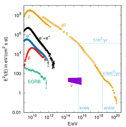
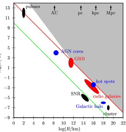
Figure 1: Left panel: Summary of intensity measurements $E^{2}I(E)$ of CR nuclei and protons (orange), electrons plus positrons (black), positrons (blue), antiprotons (red) , neutrinos (magenta) and diffuse photons (green). Right panel: Magnetic field strength $B$ versus size $R$ of various suggested CR sources; adapted from Refs. [29, 30].

Cosmic rays interacting with gas or background photons produce neutral and charged pions whose decays in turn lead to secondary high-energy photons and neutrinos. The combined study of potential CR sources using charged CRs together with photons and neutrinos has developed into the field of multi-messenger astronomy [31]. Moreover, there is a close relationship with searches for gravitational waves: Many suggested CR sources tap their energy from the gravitational collapse of a compact object, which leads to the emission of gravitational waves. Vice versa it is expected that the merger of a binary system involving one or two neutron stars leads to the acceleration of high-energy particles, as it was observed for the first time in the case of GW170817 [32]: This event was observed extensively in the optical, x-ray and gamma-ray part of the electromagnetic spectrum, with a spectrum characteristic for a short gamma-ray burst. In follow-up searches by the IceCube and ANTARES neutrino observatories and the Pierre Auger Observatory, no neutrinos consistent with this event were found.

Notation

Many quantities in CR physics can be approximated by broken power laws. In general, we will denote the power law for the observed intensity as $I({\cal R})\propto{\cal R}^{-\alpha}$, for the injection spectrum as $Q({\cal R})\propto{\cal R}^{-\beta}$, for the diffusion coefficient as $D({\cal R})\propto{\cal R}^{\delta}$ and the power spectrum of the turbulent magnetic field as ${\cal P}(k)\propto k^{-\gamma}$. Depending on the context, we will prefer different energy variables: Both the acceleration and diffusion in magnetic fields of CR nuclei depends only on their rigidity ${\cal R}$, which favours this variable for the discussion of CR propagation. The energy per nucleon $E/A$ is conserved in spallation reactions and therefore convenient to use when CR spallation plays a major role. Direct detection experiments present their data often in terms of the kinetic energy $E_{\rm kin}=E-Am_{p}$. Finally, at the highest energies the mass number $A$ cannot be determined reliably and one uses therefore the total CR energy $E$.

Emphasis and structure

We discuss CRs with rigidity above ${\cal R}\simeq 20$ GV up to the highest energies observed. As a comparison of, e.g., electron spectra at different times in the Solar cycle shows, the differences above this rigidity are negligible relative to experimental uncertainties. Our choice for the lower limit allows us therefore to neglect the effect of solar modulations. We concentrate on the propagation of CRs and the production of secondaries, omitting details of the acceleration process in the sources. Instead we concentrate in this review on models aiming to explain recent experimental results on the observed CR fluxes: In the energy range below the knee, we discuss mainly models which were suggested as solution to the rise in the positron fraction, the breaks and the non-universality of the CR nuclei spectra. In the case of extragalactic CRs, measurements of the CR dipole and the mass composition favour a low transition energy between Galactic and extragalactic CRs and a mixed composition. Thus we concentrate on models able to explain the ankle as a feature of the extragalactic CR spectrum.

For more general overviews and the topics neglected we recommend the following resources: The textbooks [33, 34] give a comprehensive introduction into the astrophysics of CRs. They are nicely supplemented by the textbook [35], which contains an up-to-date discussion of observations and an introduction to the development of extensive air showers. The effect of solar modulations on low-energy CRs is thoroughly discussed in Ref. [36]. Diffusive shock acceleration is reviewed in the classic work [20], while more recent developments are covered, e.g., in Refs. [37, 38]. The standard diffusion approach to the propagation of Galactic CRs has been described in detail in the textbooks [33, 34]; a discussion of the numerical approach used e.g. in GALPROP and its main results is given in Ref. [39]. Gamma-ray studies using Cherenkov telescopes and satellite detectors like Fermi-LAT which have revealed important informations on CR sources are reviewed in Refs. [40, 41, 42]. Recent reviews which provide additional details on ultrahigh energy cosmic rays, in particular their mass composition and source candidates, are Refs. [43, 44]. Some historical background can be found in Refs. [45, 46, 47, 48].

In a scenario alternative to the acceleration of CRs in astrophysical sources, CRs are produced in decays or annihilations of relic particles. While this possibility is of importance for the search for particle physics beyond the standard model, it can give only a subdominant contribution to the observed CR flux: The main predictions of this scenario—a flat energy spectrum ($\propto 1/E^{1.9}$) of the decay products, a large photon fraction, equal matter and antimatter fluxes, and the (almost) absence of nuclei [49]—constrain this contribution e.g. in the energy range $10^{18}$–$10^{19}$ eV to be less than 0.1% of the total CR flux [50]. In the PeV range, it has been suggested that the diffuse neutrino flux observed by IceCube is generated by decays of dark matter particles [51]. Below TeV energies, the search for dark matter in the form of weakly interacting massive particles is a very active field, and possible connections to some anomalies in CR physics are reviewed, e.g., in Ref. [52].

We start Section 2 with a short review of our knowledge of the regular and turbulent component of the Galactic magnetic field, followed by a description of our local environment, the Local Bubble. The standard approach to CR propagation in the Galaxy based on diffusion models, the necessary inputs and the basic results are described next. Then we discuss evidence that CRs diffuse strongly anisotropically, and the resulting impact on the number of CR sources contributing to the locally observed flux. After a review of the main experimental results and the observational anomalies which have appeared during the last 10 years, we discuss models suggested to explain these anomalies.

Section 3 is devoted to the knee in the CR spectrum. We start with a discussion of observations of the knee in the all-particle spectrum and of knee structures in the spectra of nuclear groups. Then we present models which explain the knee, either by the maximal energy of different source populations or by propagation effects.

In Section 4, we discuss ultra-high energy cosmic rays (UHECR). After a discussion of measurements of the energy spectrum, we present results on the mass composition of UHECRs. Then we discuss secondary gamma-rays and neutrinos produced by UHECRs, before we review recent results on anisotropies. Next we combine the experimental evidence presented to argue that the transition between Galactic and extragalactic CRs happens at a relatively low energy, and agrees with a spectral feature called the second knee around $E\approx 5\times 10^{17}$ eV. We then discuss UHECR models which are able to explain the presented data on the spectrum, composition and the transition energy. Finally, we summarize and conclude in section 5.

2 Cosmic rays below the knee

Cosmic rays are measured locally, with the two Voyager satellites as the most distant experiments from Earth as the only exceptions. While these two satellites have started to probe the conditions outside the heliosphere, photons and neutrino observations provide in addition directional information about CRs and the physical processes taking place along the observed line-of-sight. Connecting these and the local measurements to the physics occurring in CR sources requires an accurate modelling of CR transport. Since the turbulent component of the Galactic magnetic field (GMF) scatters efficiently CRs, they perform a random walk and escape only slowly from the Galaxy. Before they escape, they cross many times the Galactic disk producing secondary CRs in hadronic interactions with gas. Additionally, CRs accumulate a grammage in their source region which typically has an increased density compared to the average density in the Galactic disk. As a result of these interactions, the abundance of elements which are produced rarely in big-bang and stellar nucleosynthesis like the lithium-beryllium-boron group or titanium is strongly enhanced in CRs, cf. with Fig. 2. The production of these secondaries provides an important handle to constrain the parameters of a given propagation and source model. Therefore we review first the properties of the GMF which determines the propagation of Galactic CRs, before we discuss the diffusion approach which has become the standard method to study Galactic CR propagation. Then we describe several observational anomalies, i.e. deviations from the “naive” expectations in the simplest diffusion picture, which have appeared as the precision of new experiments increased in the last decade. Finally, we critically discuss in this section some of the solutions proposed as explanations for these anomalies.

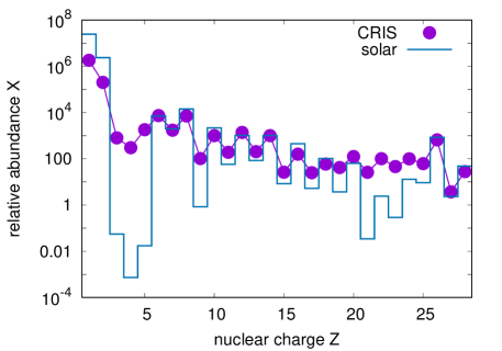
Figure 2: Relative abundances $X$ normalised to $X({\rm Si})=1000$ for the proto-sun (solar system abundances) from Ref. [53] shown as boxes versus the abundances in CRs measured by BESS [54] and CRIS [55, 56].

2.1 Galactic magnetic field and our local environment

Galactic magnetic field

The observed distribution of CR arrival directions is highly isotropic, with deviations from isotropy of only few parts in $10^{3}$ up to PeV energies. Since Galactic CR sources are strongly concentrated in the Galactic disc, an efficient mechanism for the isotropisation of the CR momenta exists. Agents of this isotropisation are turbulent magnetic fields, since CRs scatter efficiently with field modes whose wavelength matches their Larmor radius $R_{\rm L}$.

The magnetic field $\boldsymbol{B}$ can be divided into a regular component which is ordered on large scales and a turbulent component. The turbulent magnetic field satisfies $\left\langle\boldsymbol{B}(\boldsymbol{x})\right\rangle=\mathbf{0}$ and $\left\langle\boldsymbol{B}(\boldsymbol{x})^{2}\right\rangle\equiv B_{\rm rms}^{2}$, where $\langle\cdot\rangle$ denotes the ensemble average. Decomposing the turbulent field in Fourier modes with wave-vector $\boldsymbol{k}$, it can be characterised by its power spectrum $\mathcal{P}(\boldsymbol{k})$ which determines the magnetic energy density per mode $\boldsymbol{k}$. Depending on its effect on observables, the turbulent field can be split further into an anisotropic and an isotropic component.

Turbulent magnetic fields in the interstellar medium (ISM) are produced and shaped by two dominant processes: the tangling and the compression of the mean field by mass flows as, e.g., stellar winds and supernova shocks, and the action of the fluctuation dynamo [57]. In the first case, the energy in the turbulent field is injected at large scales $L_{\max}$ of order 1–100 pc. Then the energy cascades to smaller scales until it dissipates at the damping scale $L_{\min}$, which could be as low as an astronomical unit.

Turbulent fields are often modelled as Gaussian random fields, in which case all the information on the magnetic field is encapsulated in the two-point correlation function $\left\langle\boldsymbol{B}(\boldsymbol{x})\boldsymbol{B}(\boldsymbol{x}^{\prime})\right\rangle$. The correlation length $L_{\rm c}$ of the field determines the scale $k_{\rm c}=2\pi/L_{\rm c}$ above which approximately half of the energy density of the turbulent field resides. In the case of a Gaussian random field with an isotropic power-law spectrum $\mathcal{P}(k)\propto k^{-\gamma}$, it is equal to

$$L_{\rm c}=\frac{L_{\max}}{2}\>\frac{\gamma-1}{\gamma}\>\frac{1-(L_{\min}/L_{\max})^{\gamma}}{1-(L_{\min}/L_{\max})^{\gamma-1}}\simeq\frac{L_{\max}}{2}\>\frac{\gamma-1}{\gamma},$$ (2)

where the approximation is valid for $L_{\max}\gg L_{\min}$ and $\gamma>1$. With $\gamma=5/3,\,3/2$ and 1 respectively for Kolmogorov [58], Iroshnikov-Kraichnan [59, 60] and Bohm turbulence, it follows $L_{\rm c}=L_{\max}/5$, $L_{\rm c}=L_{\max}/6$ and $L_{\rm c}=L_{\min}$. The turbulent fields obtained in MHD simulations are not Gaussian random fields but intermittent: Magnetic fields generated via the induction equation by the random motion of the plasma reflect the non-Gaussian correlations in the plasma velocity. For instance, Ref. [61] finds that magnetic structures occupy a smaller proportion of the volume as the magnetic Reynolds number—which controls the relative effects of advection and diffusion—increases. It has been argued that this effect reduces on average the deflections of CRs scattering on magnetic irregularities and enhances anisotropies in the CR propagation [61]. How important the consequences of non-Gaussianity on the propagation of CRs in the Milky Way are is, however, largely unexplored. For a proper assessment, self-consistent MHD simulations including the CR fluid would be required.

Observations of fluctuations in the thermal electron density $n_{e}$ show that the corresponding power spectrum $\mathcal{P}(k)$ follows over twelve decades $\mathcal{P}(k)\propto k^{-5/3}$ [62], i.e. the slope agrees with the one predicted by Kolmogorov [58]. Since electrons may not be purely passive tracers for the magnetic field, direct measurements of the magnetic turbulence are however necessary. The only direct measurements of the magnetic field in the local ISM have been performed by a magnetometer on board of Voyager 1: These measurements are consistent with Kolmogorov turbulence and, extrapolated to larger scales, a maximal scale of $L_{\max}\simeq 10$ pc [63]. Alternatively, one can combine different probes along a line-of-sight to break the degeneracy between various parameters. For instance, combining Faraday rotation measurements, ${\rm RM}\propto\int{\rm d}\boldsymbol{s}\cdot\boldsymbol{B}n_{e}$, with emission measurements, ${\rm EM}\propto\int{\rm d}s\,n_{e}^{2}$, one can infer the power spectrum of the turbulent magnetic field and the electron density separately. On scales $L\raise 1.29167pt\hbox{$\;<$\kern-7.5pt\raise-4.73611pt\hbox{$\sim\;$}}4$ pc, the power-spectrum of magnetic turbulence is consistent with three-dimensional Kolmogorov turbulence [64, 65]. Its correlation length grows from $\sim 1$ pc in the spiral arms and $\sim 10$ pc in the interarm regions of the Galactic disk to $\sim 100$ pc in the halo according to Refs. [65, 66]. The strength of the Kolmogorov part of the turbulent field was estimated as $B_{\rm rms}\simeq 0.6\mu$G [64] with a maximal scale of $L_{\max}\simeq 4$ pc. Above this scale, the slope of the turbulence decreases, being close to $\alpha\simeq 2/3$ between $4\,{\rm pc}<L<(70-100)$ pc. Presumably, this break in the power spectrum indicates a change from isotropic to anisotropic turbulence, when the field components along the regular field are enhanced. For the propagation of CRs, such a field acts locally like a part of the ordered field.

The magnetic field of the Milky Way is concentrated in the Galactic disk, and its regular component approximately follows the spiral arms. These arms are commonly modelled as logarithmic spirals. While a magnetic field reversal on kpc scales has been unambiguously detected from pulsar RMs, observations have not determined yet whether this reversal is a global one following the spiral arms, or whether it is a local feature. The GMF has an out-of-plane component, presumably similar to the X-shaped halo fields detected in nearby edge-on spiral galaxies. The strength of the coherent magnetic field as derived from pulsar RMs is $\simeq 2\mu$G, generally consistent with values obtained modelling synchrotron radiation. The total magnetic field strength is $\simeq 6\mu$G at the Solar radius, increasing to $\simeq 10\mu$G at a Galacto-centric radius of 3 kpc. Both the strength and the scale height of the halo field are rather uncertain, with estimates for the strength varying between $\simeq 2\mu$G and $\simeq 12\mu$G and for the scale height between $\simeq 1-5$ kpc from pulsar RMs and $\simeq 5-6$ kpc from synchrotron emissivities; for reviews of the GMF see, e.g., Refs. [67, 68, 69].

Current models of the GMF like those of Refs. [70, 71, 72] reproduce the Faraday RM data and synchrotron emission maps to which they were fitted, although the GMF morphology differs substantially between these models. This implies, e.g., that it is at present not possible to correct the deflection of a UHECR by the GMF in a model-independent way. In contrast, CR propagation at lower energies depends mainly on global features of the GMF, as, e.g., the average escape time from the Galactic disk, and the differences between these models play a smaller role.

Despite the variations between current GMF models and the relative large uncertainties in the estimates of their parameters, we can draw a few important conclusions: First, a significant contribution to the total field strength is the anisotropic turbulent (also called “ordered random” or “striated”) field whose fluctuations have typical length scales larger than a pc. Thus for the propagation of CRs with energies below the knee, this field acts locally like a part of the regular field. Second, the strength of the Kolmogorov part of the turbulent field at smaller scales—which is relevant for the scattering and isotropisation of CRs at these energies—is smaller than the regular field. As a consequence, CR propagate preferentially along the ordered field, and therefore CR transport is anisotropic. Moreover, the escape of CRs from the Galactic disk depends strongly on the presence of an out-of-plane component of the regular magnetic field.

While it is natural to connect the isotropic Kolmogorov component to the hydrodynamic turbulence in the ionized gas, the anisotropic component could be generated by shock waves compressing a previously isotropic random field, or by Galactic shear motions of the gas. Another cause for an anisotropy in the turbulent magnetic field might be that the regular field modifies the cascading of magnetic modes from large to small scales. An example for such a model is Goldreich-Sridhar turbulence [73], where the power spectrum in the perpendicular direction is Kolmogorov-like, and that in the parallel direction is $\propto k^{-2}$. While such a type of turbulence is more isotropic on scales close to the outer scale $L_{\max}$, it becomes increasingly anisotropic for large wave-vectors. Thus such a behaviour is opposite to the one observed, where the anisotropic field dominates the large length scales. If the turbulence is compressible, fast magnetosonic waves may exist in addition. Because of their smaller degree of anisotropy, these waves may increase CR scattering as argued, e.g., in Ref. [74]. Finally, we note that at sufficiently low energies the magnetic turbulence generated by CRs in form of Alfvén waves may become the dominating contribution to the turbulent field.

Our local environment

The Sun resides inside a bubble of hot, tenuous plasma called the Local Bubble. Such superbubbles are created around OB associations, when the wind-blown bubbles of the individual stars encounter each other as they expand and merge to form a single superbubble [75, 76]. Once the massive O and B stars explode at the end of their fusion cycle as core-collapse supernovae, shock waves are injected into the ISM. These shocks expand quickly until they reach the bubble wall where they are typically stopped [77]. Therefore they do not form visible supernova remnants (SNR), but instead power the expansion of the superbubble in the ISM.

The Local Bubble extends roughly 200 pc in the Galactic plane, and 600 pc perpendicular to it, with an inclination of about $20^{\circ}$ [78]. Observations [79, 80] and simulations [81, 82] show that the bubble walls are fragmented and twisted. Moreover, outflows away from the Galactic plane may open up the bubble [81]. The Local Bubble abuts with the Loop 1 superbubble, and with another bubble towards the direction of the Galactic center [83].

The magnetic field inside the bubble wall is expected to be enhanced by the shocks compressing the ISM. In Ref. [84], the Chandrasekhar-Fermi method was used to derive $B_{\perp}=(8^{+5}_{-3})\mu$G for the strength of the magnetic field in the wall of the Local Bubble. Since this analysis is only sensitive to the field component perpendicular to the line-of-sight, the derived value can be seen as a lower limit on the strength of the magnetic field in the wall. A similar result was obtained in Ref. [85] which measured Faraday RMs towards the Galactic south and north pole. These authors used their upper limit of $|{\rm RM}|\sim 7$rad/m^-2 towards the bubble wall to derive the magnetic field inside the wall. Modelling the Local Bubble as a cylindrical shell with radius 85 pc and a wall thickness of 4 pc, they derived $B\simeq 9\mu$G inside the bubble wall, consistent with the value obtained in Ref. [84]. In Ref. [79], evidence for a systematically varying field strength in the bubble wall was presented: Using the Chandrasekhar-Fermi method, one set of values around $B_{\perp}\simeq 8\mu$G, and another one with strengths about three times higher, and up to about $40\mu$G was determined. Such a variation is not too surprising in view of the fragmented structure of the bubble wall and may be caused by an additional compression of the wall by interactions of the outflow in the Local Bubble and opposing flows by surrounding OB associations.

The strength and direction of the magnetic field inside the Local Bubble are only poorly constrained by observations: For instance, the difference between the flow directions of interstellar He and H has been explained by a mismatch of the local magnetic field direction and the flow of the ISM. Using Voyager data, Ref. [86] deduced $B\simeq 2\mu$G and an angle of $\alpha=30^{\circ}-60^{\circ}$ between the local magnetic field direction and the flow of the ISM. In Ref. [87], theoretical MHD models of the heliosphere were used to predict the Ly$\alpha$ absorption along various lines of sight for different configurations of the local magnetic field. Comparing the predicted and observed Ly$\alpha$ spectra, models with $B\simeq 1.25-2.5\mu$G and $\alpha=15^{\circ}-45^{\circ}$ were found to fit best the data. While these observations constrain the very local magnetic field, the field between the bubble wall and the heliosphere is more difficult to determine. In Ref. [88], Planck observations of dust polarised emission were fitted to a toy model describing the geometry of the magnetic field in the bubble. While dust polarised emission provides no information about the strength of the field, the direction of the local magnetic field was determined as $(l,b)=(70^{\circ}\pm 11^{\circ},43^{\circ}\pm 8^{\circ})$ in the northern and $(l,b)=(78^{\circ}\pm 8^{\circ},-14^{\circ}\pm 18^{\circ})$ in the southern Galactic polar caps. The large difference between the two directions indicates that the magnetic field in the Local Bubble is highly distorted.

Note also that the argument raised in Ref. [89] that a magnetic field of up to $7\mu$G is required in the Local Bubble to counter-balance the thermal pressure exerted by the enclosing hot X-ray gas is obsolete: First, the discovery of X-ray emission associated with charge exchange between solar wind ions and heliospheric neutrals has reduced the need of non-thermal pressure support of the LB [90]. Second, a contamination from X-ray emission from the walls of the Local Bubble [90], and an improper assumption of collisional ionization equilibrium [91] may invalidate the pressure balance argument of Ref. [89].

2.2 Standard approach to Galactic cosmic ray propagation

2.2.1 Method and inputs

In the standard approach to Galactic CR propagation, the $N$-particle phase space distribution of CRs is approximated as a macroscopic fluid. Then the time evolution of individual CRs propagating under the influence of the Lorentz force is replaced by a diffusion process. Such a replacement corresponds to a coarse-graining of CR trajectories on length scales $\sim L_{\rm c}^{\alpha-1}R_{\rm L}^{2-\alpha}$. For CRs with rigidity ${\cal R}=100$ TV and Kolmogorov turbulence with a correlation length of order 10 pc, the length $L_{\rm c}^{2/3}R_{\rm L}^{1/3}$ corresponds to pc scales. Note that particles with the same rigidity moving under the influence of only the Lorentz force follow the same trajectories in phase space. As a consequence, both diffusion in space and in momentum (i.e. (re-) acceleration) proceed independently of the mass number of CR nuclei. Therefore one expects the same CR spectra for different CR primaries, if they are expressed as function of rigidity and interactions can be neglected.

The (spatial) diffusion tensor

$$D_{ij}(\boldsymbol{x}_{0},{\cal R})=\lim_{t\to\infty}\frac{1}{2Nt}\sum_{a=1}^{N}(x_{i}^{(a)}-x_{i,0})(x_{j}^{(a)}-x_{j,0})$$ (3)

can be determined numerically following the trajectories $x_{i}^{(a)}(t)$ of $N\gg 1$ CRs injected at $\boldsymbol{x}_{0}$ for a given magnetic field configuration [92, 93, 94]. Since these calculations are computationally expensive, one usually employs analytical approximations instead. For instance, the connection between the diffusion coefficient $D_{\|}$ parallel to the ordered field and the power spectrum ${\cal P}(k)$ of the turbulent magnetic field can be derived analytically in the approximation of pitch-angle scattering, if the ordered field dominates at the scale considered [33]. In this case, the slope of the power spectrum ${\cal P}(k)\propto k^{-\gamma}$ determines the rigidity dependence of the diffusion coefficient parallel to the ordered field as $D_{\|}({\cal R})\propto{\cal R}^{\delta}$ with $\delta=2-\gamma$. In Ref. [39], the numerical value of $D_{\|}({\cal R})$ was estimated as $D_{\|}\simeq 2\times 10^{27}({\cal R}/{\rm GV})^{1/3}$ cm²/s for a turbulent magnetic field with $B_{\rm rms}=5\mu$G, $L_{\max}=100$ pc and Kolmogorov turbulence. In practise, most studies of CR propagation employ instead a scalar diffusion coefficient with a prescribed functional form as, e.g., $D({\cal R})=D_{0}({\cal R}/{\cal R}_{0})^{\delta}$, and determine the normalisation constant $D_{0}$ from a fit to secondary-to-primary ratios as B/C (as we will discuss in the Section 2.2.2).

The CR fluid is coupled to the ISM and can drive, e.g., Galactic winds [95, 96]. Its pressure is in rough equipartition with the magnetic and dynamical pressure in the ISM [67, 97], suggesting the dynamical importance of CRs for the ISM. Moreover, CR streaming can lead to wave turbulence and thus to the generation of turbulent magnetic field modes. As a result, CRs, the ISM and the GMF form a coupled, non-linear system which should be modelled self-consistently. For recent studies in this direction see e.g. Refs. [98, 99, 100, 101]. Considering CRs of sufficiently high energy, $E\raise 1.29167pt\hbox{$\;>$\kern-7.5pt\raise-4.73611pt\hbox{$\sim\;$}}E_{\ast}$, this coupling can be neglected because the CR density drops fast with energy. The numerical value of $E_{\ast}$ is however very uncertain. For instance, Ref. [102] argued that $E_{\ast}$ is as low as $E_{\ast}\sim 1$ GeV, i.e. the energy where a break in the diffusion coefficient both from observation of synchrotron radiation from electrons [103] and from secondary-to-primary rations was deduced [102]. In contrast, the specific model proposed in Refs. [104, 105, 106] which will be discussed as an example for the coupling between CRs and self-generated turbulence in the next subsection argues for a high value, $E_{\ast}\sim 300$ GeV.

Restricting ourselves to energies $E\raise 1.29167pt\hbox{$\;>$\kern-7.5pt\raise-4.73611pt\hbox{$\sim\;$}}E_{\ast}$, CRs can be propagated using prescribed magnetic fields and gas densities as background. Adding then also interactions, the resulting transport equation for the (differential) density $n^{(a)}(\boldsymbol{x},p,t)={\rm d}N^{(a)}(\boldsymbol{x},p,t)/({\rm d}p{\rm d}V)=4\pi p^{2}f^{(a)}(\boldsymbol{x},p,t)$ of CR particles of type $a$ is given by

$$\begin{split}\@ADDCLASS{ltx_eqn_lefteqn}$\displaystyle\frac{\partial n^{(a)}}{\partial t}-\nabla_{i}\left[D_{ij}\nabla_{j}-u_{i}\right]n^{(a)}-\frac{\partial}{\partial p}\left[p^{2}D^{(p)}\frac{\partial}{\partial p}p^{-2}n^{(a)}\right]=-\frac{\partial}{\partial p}\left(\beta^{(a)}n^{(a)}\right)$\mbox{}\hfil\\ &-\left(cn_{\rm gas}\sigma_{\rm inel}^{(a)}+\Gamma^{(a)}\right)n^{(a)}+Q^{(a)}+\sum_{b}\left[cn_{\rm gas}\int_{E}^{\infty}dE^{\prime}\;\frac{{\rm d}\sigma^{ba}(E^{\prime},E)}{{\rm d}\!E}+\Gamma^{ba}\right]n^{(b)}\,.\end{split}$$ (4)

While the first line of Eq. (4) describes the continuous time evolution of the particle density $n^{(a)}$ due to (spatial) diffusion, advection, diffusion in momentum space and continuous energy losses, the second line accounts for gain and loss processes. Particles are lost in inelastic reactions and, if they are unstable, in decays; they are injected by CR sources and produced as secondaries in interactions and decays of particles of type $b$. Most quantities, like the diffusion tensor $D_{ij}$, the advection velocity $\boldsymbol{u}$, the injection rate $Q$, the energy loss rates $\beta$, and the gas density $n_{\rm gas}$ depend on space and/or time. For instance, the spatially varying strength of the GMF will lead to changes in the diffusion tensor and the synchrotron losses. Similarly, the discrete nature of CR sources implies that their injection rate $Q$ is both space and time dependent.

In order to reduce the complexity of this coupled set of partial differential equations, one separates the problem of CR acceleration in their sources from their propagation. Thus one employs for $Q$ an ansatz for the spectrum of CRs after escape from their sources. Interactions and energy losses (except for electrons at highest energies) do not modify strongly the spectrum of primary CRs in the source and one expects therefore that they share the same rigidity spectrum. The ansatz for this spectrum is typically chosen as a power law, $Q^{(a)}({\cal R})=Q^{(a)}_{0}({\cal R}/{\cal R}_{0})^{-\alpha}\exp(-{\cal R}/{\cal R}_{\max})$, with a rigidity-dependent maximal energy $E_{\max}=Ze{\cal R}_{\max}$ and an exponential cutoff. The results from diffusive shock acceleration in the test-particle limit motivate the range $\alpha\simeq 2.0-2.2$ for the slope of the injection spectrum. However, both the back-reaction of CRs on the shock and their energy-dependent escape from their sources affect the test-particle picture and modify the CR energy spectra. A potential resurrection of the power-law spectra with $\alpha\simeq 2.0-2.2$ normally employed are the results from Ref. [107]: There it was shown that steep acceleration spectra with $\alpha>2$ are converted into an escape spectrum with $\alpha\simeq 2$. Moreover, steep acceleration spectra are required for the large maximal energies needed to explain the extension of the Galactic CR spectrum beyond the knee. Similar conclusions were obtained in Refs. [108, 109].

The relative abundances $Q^{(a)}_{0}$ of nuclei in the injection spectra are either chosen close to the Solar ones, or are determined from a fit of the produced abundances after propagation to the observed ones. Additionally, the spatial distribution of the sources has to be fixed. In most models, the injection of Galactic CRs is correlated with supernovae (SN). Therefore, the spatial dependence of $Q^{(a)}_{0}$ is normally modelled according to the observed distributions of supernova remnants (SNRs) or pulsars [110]. Often, one neglects the spiral structure of the Galactic disc as well as the enhanced SN activity in the Galactic bulge. The latter assumption is justified, because of the small volume of this region, except if one studies especially the photon emission from this region [111]. Similarly, the spiral structure is averaged out in many observational quantities, except e.g.  for high-energy electrons which can travel only short distances.

Magnetic fields are not purely static but move with a typical velocity of the Alfvén speed, $v_{A}=B/\sqrt{4\pi\rho_{\rm ion}}\simeq(10-30)$ km/s with $\rho_{\rm ion}$ denoting the mass density of ionised atoms, and thus diffusion occurs not only in space but also in momentum. This results in second-order Fermi acceleration during the propagation of CRs. The connection between the spatial and momentum diffusion coefficients is given by $D^{(x)}D^{(p)}=\varepsilon p^{2}v_{A}^{2}$, with $\varepsilon(\beta)\sim 0.1$ [33, 112]. Both analytical and numerical calculations indicate that a large fraction of the total energy in CRs is delivered by this process which is often called “reacceleration” [112]. However, reacceleration on Alfvén waves modifies the CR spectrum only at mildly relativistic energies, i.e. at energies below our interest.

Advection, i.e. the bulk motion of the ISM, competes with diffusion as an efficient way to transport CRs away from the Galactic disk. Since advection is energy independent, it is the dominating transport mechanism at sufficiently low energies. For an uniform advection velocity, flat secondary-to-primary ratios at low energies result. The observed flattening of the B/C ratio at few GeV was interpreted as evidence for advection first in Ref. [113]. However, advection is in case of Kolmogorov turbulence not necessary to reproduce the B/C data, and Refs. [114, 115] obtained zero advection velocity as their best-fit case. In a more realistic description, the advection velocity increases with the distance to the Galactic plane. Moreover, in regions of enhanced star formation activity superbubbles are formed which may open towards large Galactic latitudes. In these “Galactic fountains”, ISM and CRs may be effectively advected out of the disk [81, 98]. Note also that a $z$ dependent increase of the advection velocity $u$ can modify the energy dependence of the diffusion coefficient deduced.

Continuous energy loss processes are only important at low energies, $E\raise 1.29167pt\hbox{$\;<$\kern-7.5pt\raise-4.73611pt\hbox{$\sim\;$}}1$ GeV and, for electrons at high energies. In the latter case, the energy loss of an electron due to synchrotron radiation is given in the Thomson regime by

$$\beta\equiv-\frac{{\rm d}E}{{\rm d}t}\equiv bE^{2}=3.79\times 10^{-18}\,\frac{\rm GeV}{\rm s}\left(\frac{B}{\mu\rm G}\right)^{2}\left(\frac{E}{\rm GeV}\right)^{2}\,.$$ (5)

The losses due to inverse Compton scattering on cosmic microwave background photons and starlight can be included using $u/({\rm eV/cm^{3}})\simeq(6.3\,B/\mu{\rm G})^{2}$. As result of the losses, the energy of an electron degrades with time as $E(t)=E_{0}/(1+bE_{0}t)$, and its half-life is

$$\tau_{1/2}=1/(bE_{0})=8.35\times 10^{9}\,{\rm yr}\left(\frac{\rm\mu G}{B}\right)^{2}\frac{\rm GeV}{E}\,.$$ (6)

Thus electrons with energy 100 GeV should be injected less than 5 Myr ago. This implies in turn that the sources of high-energy electrons have to be local. Note also the difference between continuously injecting and bursting sources of electrons: In the first case, energy losses lead to a break with $\Delta\alpha=1$ in a power-law energy spectrum, while the energy spectrum of a bursting source has a sharp cutoff.

Finally, the last main ingredient in the transport equation are the particle interactions which require as input cross sections and decay rates as well as the distribution of the target material. For the latter one can use either the Galactic mass distribution derived from kinematical studies [116] or the H I distribution from radio observations [117]. The scattering and decays of CR nuclei are determined by strong interactions and nuclear effects and, at present, it is therefore not possible to calculate them from first principles. Conventionally, one calls spallation reactions those interactions where CR nuclei fragment on gas of the ISM, loosing one or more nucleons and producing thereby lighter nuclei. In particular, one can assume in spallation reactions zero energy transfer between the nuclei, if one neglects the Fermi motion of nucleons inside a nucleus. Therefore, the energy per nucleon $E/A$ is conserved in such reactions. In this approximation, only the total production cross sections $\sigma^{a\to b}$ as function of energy are required as input from experimental measurements. Still, an accurate modelling with errors smaller than, e.g., 3% of the lithium flux requires the knowledge of twelve cross sections with much improved accuracy compared to current knowledge [118]. A pilot run [119] to collect new data on nuclear fragmentation has recently been performed by the NA61/SHINE collaboration and a comprehensive measurement campaign is proposed to take place after the long shutdown 2 of the CERN accelerator facilities [120]. Since measurements cannot cover the required energy range for all relevant reactions, one has to rely on parametrisations for the spallation cross sections. Parametrisations like the one of Ref. [121] for the total inelastic cross section $\sigma_{\rm inel}^{(a)}$ and of Ref. [122] for the partial spallation cross sections $\sigma^{a\to b}$ assume that these cross sections are constant above few GeV/n. Since inelastic strong interaction cross sections grow only logarithmically at high energies, the energy range experimentally covered is too small to determine this growth given the typical experimental precision. Using instead Monte Carlo simulations like QGSJET-II-04 [123, 124] for the determination of, e.g., the total inelastic cross section $\sigma_{\rm inel}$ of ¹²C, one finds an increase from 200 mbarn to 255 mbarn moving from 10 GeV/n to 1 TeV/n. Theoretically, one expects that the fragmentation cross sections $\sigma^{a\to b}$ grow with energy proportionally to the total inelastic cross section $\sigma_{\rm inel}$. Thus constraining the slope of the diffusion coefficient $D({\cal R})\propto{\cal R}^{\delta}$ using constant fragmentation cross sections may overestimate $\delta$ by 0.05, cf. with Eq. (11).

At energies $E/A\raise 1.29167pt\hbox{$\;>$\kern-7.5pt\raise-4.73611pt\hbox{$\sim\;$}}{\rm few}$ GeV, it is not possible to separate between spallation reactions and interactions with additional particle production: Practically all inelastic scatterings are a combination, where the primary nucleus fragments partly into pieces $j$ with energy $\simeq E/A_{j}$, while a fraction of its energy is converted into additional mesons and baryons. For a sufficiently steeply falling CR primary spectrum, the products of these hard “sub-reactions” can be neglected, keeping track only of those secondaries one is interested in, such as antiprotons, positrons, photons or neutrinos.

2.2.2 Basic results

Cosmic ray fluxes

In order to solve the set of transport equations, several approximations are usually made. First, one notes that the measured ratios of radioactive CR isotopes like Be¹⁰ with a lifetime of $\simeq 1.6$ Myr to the stable Be⁹, and of secondary-to-primary ratios like B/C indicate a residence time of CRs of order $\tau_{\rm esc}\simeq{\rm few}\times 10^{7}{\rm yr}\left({\cal R}/5\,{\rm GV}\right)^{-\beta}$ with $\beta\simeq 1/3$ [125, 126]. If one then assumes that the main CR sources are SNe injecting $\simeq 10^{50}$ erg every $\sim 30$ yr in the form of CRs, then the flux from some $10^{4}$ sources accumulates at low rigidities, forming a “sea” of Galactic CRs. Since many sources contribute, the discrete nature of the CR sources can be neglected. This allows one to consider the stationary limit of Eq. (4) and to use a smooth, time-independent source distribution $Q(\boldsymbol{x})$. As a second approximation, one also neglects the spatial dependence of the diffusion term, replacing the Galaxy by a cylinder with uniform propagation properties for CRs. Finally, one replaces often the tensor $D_{ij}$ by a scalar diffusion coefficient $D$, assuming that the turbulent field dominates relative to the regular field. Note that the last two approximations clearly contradict our knowledge of the GFM which indicates a strong variation of the magnetic field strength, both as function of galactocentric radius and distance to the Galactic plane, as well as an anisotropic diffusion of CRs. These approximations imply that the fit results derived in such diffusion models for, e.g. the normalisation $D_{0}$ of the diffusion coefficent, can be seen only as effective parameters.

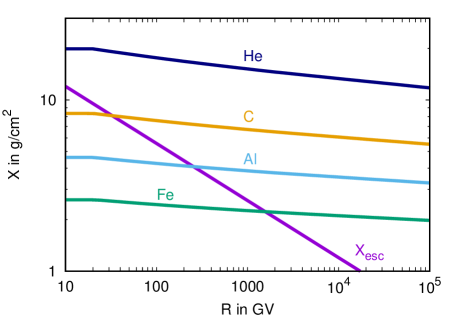
Figure 3: Interaction depths $X^{a}=m_{p}/\sigma_{\rm inel}^{(a)}$ calculated with QGSJET-II-04 [123, 124] and the escape depth $X_{\rm esc}=X_{0}({\cal R}/{\cal R}_{0})^{-1/3}$ as function of rigidity ${\cal R}$.

The basic behaviour of the solutions obtained solving numerically the coupled transport equations (4) using these appproximations can be understood from a simple leaky-box model: This model assumes that CRs inside a uniform confinement volume, e.g. a CR halo with height $h$, have a constant escape probability per time which is small, such that $\tau_{\rm esc}\gg h/c$. Neglecting all other effects in Eq. (4), these equations reduce to

$$\frac{\partial n^{(a)}}{\partial t}=\frac{n^{(a)}}{\tau_{\rm esc}}=D\Delta n^{(a)}\,,$$ (7)

and hence one can replace the diffusion term by $n^{(a)}/\tau_{\rm esc}$. If we consider now the steady-state solution, $\partial n^{(a)}/\partial t=0$, then we obtain

$$\frac{n^{(a)}(E)}{\tau_{\rm esc}}=Q^{(a)}-\left(cn_{\rm gas}\sigma_{\rm inel}^{(a)}+\Gamma^{(a)}\right)n^{(a)}(E)+cn_{\rm gas}\sum_{b}\int_{E}^{\infty}{\rm d}\!E^{\prime}\;\frac{{\rm d}\sigma_{ab}(E^{\prime},E)}{{\rm d}\!E}\>n^{(b)}(E^{\prime})\,.$$ (8)

For stable primary types like protons or ⁵⁶Fe, the decay term vanishes and production via fragmentation can be neglected. Introducing $X_{\rm esc}=c\rho\tau_{\rm esc}$ and $X^{(a)}=m_{p}/\sigma^{(a)}_{\rm inel}$ as the amount of matter traversed by a relativistic particle before escaping and interacting, respectively, it follows

$$n^{(a)}=\frac{Q^{(a)}\tau_{\rm esc}}{1+X_{\rm esc}/X^{(a)}}\,.$$ (9)

The interaction depths $X^{(a)}$ are compared for some common nuclei in Fig. 3 to the escape depth $X_{\rm esc}=X_{0}({\cal R}/{\cal R}_{0})^{-\delta}$, for which we assumed Kolmogorov turbulence, $\delta=1/3$, and $X_{0}=12$ g/cm² at ${\cal R}_{0}=10$ GV. For protons and helium, $X_{\rm p}>X_{\rm He}\gg X_{\rm esc}$ for all energies, and thus

$$n_{\rm p}=Q_{\rm p}\tau_{\rm esc}\propto Q_{0}E^{-(\beta+\delta)}\,.$$ (10)

Hence the injection spectrum of protons and helium should be flatter than the one observed: For Kolmogorov turbulence, $\delta=1/3$, the observed slope of the proton spectrum $\alpha=2.7$ requires the slope $2.4$ for the injection spectrum.

For the other extreme case, iron, the interaction and escape depths are equal around ${\cal R}\simeq 2000$ GV. Hence at lower rigidities, iron nuclei are destroyed by interactions before they escape, $X_{\rm Fe}\ll X_{\rm esc}$, and therefore the iron spectrum reflects the generation spectrum, $n_{\rm Fe}\propto Q_{\rm Fe}$. Starting from the energy where $X_{\rm Fe}\approx X_{\rm esc}$, the iron spectrum should become steeper. The observed iron spectrum is indeed flatter at low energies than, e.g., the helium spectrum. However, the expected steepening at ${\cal R}\simeq 2000$ GV is absent in the data.

The density of stable secondaries like boron follows with $\Gamma=Q=0$ and as

$$n^{(a)}=\frac{X_{\rm esc}\sum_{b}\sigma^{ba}/m_{p}\,n^{(k)}}{1+X_{\rm esc}/X^{(a)}}.$$ (11)

Here, we have assumed that $E/A$ is used as variables which is approximately conserved in fragmentation processes. Secondary-to-primary ratios like B/C are thus given by

$$\frac{n_{\rm B}}{n_{\rm C}}=\frac{X_{\rm esc}}{1+X_{\rm esc}/X^{(B)}}\sum_{k>B}\frac{\sigma^{k\to B}}{m_{p}}\frac{n_{k}}{n_{C}}\propto{\cal R}^{-\delta}\,.$$ (12)

In the last step, we have assumed energy independent fragmentation cross sections and $X_{\rm esc}/X^{(B)}\ll 1$. The latter condition is satisfied at sufficiently high rigidities, ${\cal R}\gg 30$ GV. As discussed above, the first assumption leads to an overestimation of $\delta$ by 0.05.

Thus a measurement of a secondary-to-primary ratio like B/C at sufficiently high energies allows one to determine the energy-dependence of the diffusion coefficient, constraining thereby the power-spectrum of the turbulent magnetic field modes. The most precise data on the B/C ratio are those of the AMS-02 experiment [127], which determine in Eq. (12) the slope as $\delta=0.333\pm 0.015$ using data above 65 GV. Hence the data are consistent with a Kolmogorov power spectrum of the turbulent magnetic field.

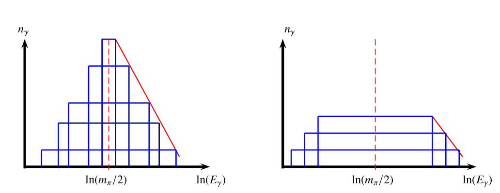
Figure 4: The photon spectrum $n_{\gamma}={\rm d}N/{\rm d}E_{\gamma}$ produced in $\pi^{0}$ decays as function of $\ln(E_{\gamma})$ for $Ap$ (left panel) and for $A\gamma$ (right panel) interaction: the total spectrum is the enveloppe (red line) of the boxes produced by pions with fixed energy.

Let us next discuss a few basic properties of the secondary fluxes of particles which are produced in hadronic interactions of CRs on gas, either directly or via the decay of mesons. Photons are mainly produced by the decay of neutral pions, $\pi^{0}\to 2\gamma$, with a flat energy spectrum ${\rm d}n/{\rm d}E_{\gamma}=\;$const. for a given pion energy. The maximal and minimal energy of these photons is $E_{\min}^{\max}=\frac{m_{\pi}}{2}\sqrt{\frac{1\pm\beta}{1\mp\beta}}$. The energy spectrum of the decay photons from pions with fixed energy ploted as function of $\ln(E_{\gamma})$ corresponds therefore to a symmetric box around half of the pion mass, cf. the left panel of Fig. 4. A signature of photons from hadronic interactions is therefore the symmetry of the photon spectra as function of $\ln(E_{\gamma})$ with respect to $m_{\pi}/2$. The low threshold and the approximate Feynman scaling for forward production spectra in hadronic interactions implies then ${\rm d}N_{\gamma}/{\rm d}E\propto{\rm d}N_{\rm CR}/{\rm d}E$. These arguments were used for the SNRs IC 443 and W44 to argue for the acceleration of CR protons in these sources [128]. Note however that these observations do not cover the peak and the low-energy side of the “pion bump” and depend therefore on the modelling of these sources.

The intensity of secondaries is suppressed relative to the one of primaries depending on the energy fraction $z=E_{s}/E_{p}$ transferred to the secondaries and the slope $\alpha$ of the primary intensity. This suppression can be accounted for in case of a power-law primary intensity, $I_{p}(E)\propto E_{p}^{-\alpha}$, by defining $Z$ factors as follows,

$$Z_{s}(E_{s},\alpha)=\int_{0}^{1}{\rm d}z\,z^{\alpha-1}\,\frac{{\rm d}\sigma_{s}(E_{s}/z,z)}{{\rm d}z}\,.$$ (13)

Here, ${\rm d}\sigma_{s}(E,z_{s})/{\rm d}z_{s}$ denotes the inclusive spectrum of secondaries. The intensity of secondaries of type $s$ is then simply given by $I_{s}(E)=c\tau nZ_{s}(E,\alpha)I_{p}(E)$ with $\tau$ as the time spent in the source region with target density $n$, if the primary intensity can be described by a power-law.

As an important example, we give in Table 1 the $Z$ factors for the production of photons in $pp$ interactions for various values $\alpha$ and photon energies $E_{\gamma}$ calculated with QGSJet-II-04 [123, 124]. Moving from a flat spectrum with $\alpha=2$ to a steep one with $\alpha=3$, the $Z$ factor decreases by a factor $\simeq 10$ and, thus, the secondary photon flux is suppressed by the same factor, $I_{\gamma}(\alpha=3)\simeq I_{\gamma}(\alpha=2)/10$. Similarly, the effect on the secondary yield of heavier primary nuclei as well as of the helium contribution in the gas depends strongly on the slope of the CR fluxes. A simple and convenient way to account for the contribution of heavier nuclei to the diffuse gamma-ray emission is provided by the nuclear enhancement factor $\varepsilon$. For the parametrisation of Ref. [129] for the CR flux, the numerical values of the enhancement factor $\varepsilon$ for the photon yield were determined as 1.87, 1.98, 2.09 for $E_{\gamma}=10,100,1000$ GeV in Ref. [130]. In general, however, production cross sections calculated for the specific primary and target nuclei should be used, which are provided e.g. by the parametrisation AAfrag [131].

$E_{\gamma}$	$\alpha=2$	$\alpha=2.2$	$\alpha=2.4$	$\alpha=2.6$	$\alpha=2.8$	$\alpha=3$
10 GeV	5.45	3.06	1.84	1.17	0.771	0.529
100 GeV	5.93	3.20	1.86	1.14	0.736	0.492
1 TeV	6.85	3.61	2.05	1.24	0.786	0.519

Table 1: $Z_{\gamma}(E_{s},\alpha)$ factor in mbarn of the reaction $pp\to X\gamma$ for different values of $\alpha$ and $E_{\gamma}$.

Note also the special case of antiproton production where the threshold energy is $E_{\rm th}=7m_{p}$. There are two main consequences of this high threshold: First, the antiproton production cross section has a rather strong dependence on the energy of the produced antiprotons up to $E_{\bar{p}}\simeq 100$ GeV. Second, the suppression of the antiproton production cross section below $E_{\bar{p}}\simeq 100$ GeV is difficult to model in Monte Carlo simulations of strong interactions, because it depends on poorly constrained details in their hadronisation procedures, for a discussion see Ref. [132]. On the other side, parametrisations of experimental data like those of Refs. [133, 134, 135] have to be extrapolated outside the measured kinematical range and rely often on physically poorly motivated assumptions. Therefore, the theoretical uncertainty in the antiproton production cross section below $E_{\bar{p}}\simeq 100$ GeV is with 20% relatively large.

Sources of CRs

The possible sources of Galactic CRs are restricted by the energy budget required to keep the energy contained in the escaping CRs stationary. The local energy density of CRs can be determined from Voyager data as $\rho_{\rm CR}\simeq 0.7$ eV/cm³ [112]. If CRs are confined for the time $\tau$ inside the volume $V$ containing the gas mass $M$, they cross the grammage $X=c\tau M/V$. Combining the measured grammage, $X\simeq 10$ g/cm², and the CR luminosity $L_{\rm CR}=\rho_{\rm CR}V/\tau$ leads to

$$L_{\rm CR}=\rho_{\rm CR}\frac{cM}{X}\simeq 5\times 10^{40}{\rm erg/s}$$ (14)

using $M=5\times 10^{9}M_{\odot}$.

The classic source class suggested first by Baade and Zwicky are SNe [10]: In a successful core-collapse SN around $10\,M_{\odot}$ are ejected with velocities $v\sim 5\times 10^{8}$ cm/s. Assuming $1/(30\,$yr) as SN rate in the Milky Way, the average output in kinetic energy of Galactic SNe is $L_{\rm SN,kin}\sim 3\times 10^{42}$ erg/s. Hence, if the remnants of SNe can accelerate particles with an efficiency $O(0.01)$, they could explain the bulk of Galactic CRs. Note that an efficient magnetic field amplification which is required such that SNe can accelerate CRs up to the knee and beyond implies that CRs carry 20–30% of the initial kinetic energy of the SNe [25, 24]. Thus it is sufficient that a subset of all core-collapse SNe accelerates CRs up to the end of the Galactic CR spectrum.

These energy considerations make SN explosions a very probable energy source for Galactic CRs. However, core collapse SN explosions are not randomly distributed in the Galaxy, since the majority of core-collapse SN progenitors belong to OB associations, which are formed from the collapse of a giant molecular cloud within a short time scale. Therefore several tens of SNe occur within a few million years inside a superbubble created by the strong winds of the massive stars in the OB association. The larger dimensions of superbubbles, the presence of turbulence stirred by the stellar winds and of multiple shocks promote superbubbles to attractive acceleration sites reaching PeV energies [136]. Evidence for CR acceleration in superbubbles comes from the the so-called superbubble model for Li, Be and B production [137]. This model proved capable of accounting for all the current observational constraints pertaining to the nucleosynthesis and evolution of light element: In particular, it explains the observed very efficient production of Li, Be and B in the early Galaxy, when C and O nuclei were still very rare. Another consequence would be a substantial enrichment of CRs by freshly synthesized nuclei, from SN ejecta and stellar winds. This might offer a natural way to explain the large ²²Ne/²⁰Ne ratio observed in CRs [138] or the hardening the CR spectra of heavier elements [139, 140].

In a related scenario, most massive stars in an OB association explode before their winds merged and the superbubble forms only later. If the kinetic energy of such a SN is sufficiently large, $E_{\rm kin}\raise 1.29167pt\hbox{$\;>$\kern-7.5pt\raise-4.73611pt\hbox{$\sim\;$}}10^{51}$ erg, and the magnetic field strong, diffusive drift acceleration may be operating additionally to diffusive shock acceleration. As a result, massive stars exploding into their winds may able to accelerate CRs up to the ankle, for a detailed review of this option see Ref. [141]. Observations of radio SNe in the starburst galaxy M82 are consistent with the strong magnetic fields required in this scenario [142]. Moreover, they find large shock velocities, $v_{\rm sh}\simeq 0.1c$, suggesting that these sources can accelerate CR protons beyond the knee.

Another interesting test of the SN hypothesis has been recently performed in Ref. [143]: Using gamma-ray observation of the Constellation III region in the Large Magellanic Cloud, it was argued that SNe are favoured compared to preceding stellar winds as a site of CR acceleration. Moreover, it was shown that the energy injected in CRs equals $(1.1_{-0.2}^{+0.5})\times 10^{50}$ erg/supernova, with a power-law spectrum and slope $2.09_{-0.07}^{+0.06}$. Thus both the energy and the slope match well with the idea of shock acceleration in SNR.

A nova explosion produces similarly to a SN an expanding shell, however, with a reduced energy of $\sim 10^{46}-10^{47}$ erg. Since the frequency of nova explosion is 100/yr in the Milky Way, the total energy input per time by novae is similar or larger than the one of SNe. Thus it is possible to associate nova with a steep CR component having a maximal rigidity of 200 GV [144]. In contrast, Gamma-Ray Bursts (GRB) are potential CR sources with a high energy output, but a small rate $\raise 1.29167pt\hbox{$\;<$\kern-7.5pt\raise-4.73611pt\hbox{$\sim\;$}}10^{-4}/$yr. In Ref. [145], it was argued that the Galactic CR flux above the knee could be caused by a single Galactic GRB $\sim 500$ pc away that took place around 200,000 yr ago. In Refs. [146, 147], it was suggested that even the observed UHECRs could be explained by a Galactic GRB. Common to both works is that the propagation of CRs was treated in a simplified diffusive approach which is not justified any more at these energies. Therefore, the conclusions of these works should be taken with caution.

The Galactic center (GC) with its supermassive black hole is another potential site of CR acceleration. While the GC at present is quiet, an active episode in the past has been connected to the creation of the Fermi Bubbles. For instance, Ref. [148] estimated the average energy output of the GC as $(1-7)\times 10^{42}$ erg/s, what exceeds the energy output of SNe. In Ref. [149], it was shown that particles accelerated during such active episodes around the GC can account for a significant fraction of the locally observed CRs with energies up to knee, if the diffusive halo is large and the slope of the diffusion coefficient is high, $\delta=0.5$. Since electrons and positrons lose energy fast as they propagate, the GC can only contribute secondary $e^{\pm}$. Therefore additional local sources of electrons and positrons have to contribute the observed high-energy part of the lepton spectra in this scenario.

Challenges for the simple diffusion model

The diffusion approach based on the approximations described above has been sufficient to describe the bulk of experimental data obtained until $\simeq 2005$. With the increased precision of newer experiments like the CREAM balloon detector, the PAMELA and Fermi satellites or AMS-02 on the International Space Station several discrepancies have emerged. These observational anomalies and ideas for their solutions will be described in the next two subsections. Before that we will discuss a more conceptional challenge for the approximations employed in the standard diffusion approach [150].

Figure 5: The CR diffusion coefficient in pure isotropic Kolmogorov turbulence with $L_{\max}=25$ pc and for four values of The asymptotic behaviours at low and high energies are shown with the solid lines.

In the diffusion picture, one can model the propagation of CRs as a random walk with an energy dependent effective step size. For a pure isotropic random field, one expects therefore as functional dependence of the diffusion coefficient

$$D=\frac{cL_{0}}{3}\left[(R_{\rm L}/L_{0})^{2-\gamma}+(R_{\rm L}/L_{0})^{2}\right],$$ (15)

where the condition $R_{\rm L}(E_{\rm tr})=L_{0}$ determines the transition from small-angle scattering with $D(E)\propto E^{2}$ to large-angle scattering with $D(E)\propto E^{2-\gamma}$. At even higher energies, CRs enter the ballistic regime and the concept of a diffusion coefficient becomes ill-defined.

The numerical value of $L_{0}$ should scale with the correlation length as $L_{0}\propto L_{\rm c}$, but the proportionality factor has to be determined numerically. In Refs. [93, 150], it was found that $L_{0}\simeq L_{\rm c}/(2\pi)$ provides a good fit to their numerical results. The presence of the factor $1/(2\pi)$ becomes evident recalling that we compare in Eq. (15) the linear length $L_{0}$ with the radius $R_{\rm L}$. Numerically, the transition energy is given by

$$E_{\rm tr}=2\times 10^{14}{\rm eV}\>(L_{\rm c}/{\rm pc})\>(B/{\rm\mu G})\,.$$ (16)

Note that, for $L_{\rm c}\sim{\rm few}$ pc and $B\sim{\rm few}\,\mu$G, the transition energy $E_{\rm tr}$ is in the knee region. Thus the change in CR propagation at $E_{\rm tr}$ may be a possible reason for the spectral break at the knee.

In Fig. 5, we show the diffusion coefficient calculated using Eq. (3) for a pure random field following Kolmogorov turbulence with $L_{\max}=25$ pc for various field strengths. The transition between the asymptotic low-energy ($D\propto E^{1/3}$, large-angle scattering) and high-energy ($D\propto E^{2}$, small-angle scattering) behaviour is clearly visible. However, for all used field strengths the diffusion coefficients are much smaller than those extracted using, e.g., Galprop [151] or DRAGON [152] from fits to secondary-to-primary ratios like B/C: Typical values found are in the range $(3-8)\times 10^{28}$cm²/s at 10 GeV; their extrapolation to high energies is shown as green band in the figure. Requiring that the numerically determined diffusion coefficient for pure isotropic turbulence lies in this band determined from the B/C ratio, the possible range for the field strength and the correlation length of the turbulent field shown in the left panel of Fig. 6 follows: The weak field dependence of $D(E)\propto B_{\rm rms}^{-1/3}$ requires a reduction of $B_{\rm rms}$ by a factor $1/100^{3}=10^{-6}$ for Kolmogorov turbulence keeping $L_{\rm c}$ constant. Keeping instead $B_{\rm rms}\sim{\rm few}\times\mu$G, the correlation length should be comparable to the size of the Galactic halo. Using instead Iroshnikov-Kraichnan turbulence, even larger correlation lengths would be required. Therefore CR propagation has to be necessarily anisotropic, because otherwise CRs overproduce secondary nuclei like boron for any reasonable values of the strength and the correlation length of the turbulent field. Such an anisotropy may appear if the turbulent field at the considered scale does not dominate over the ordered component, or if the turbulent field itself is anisotropic.

Figure 6: Left panel: Allowed range of $B_{\rm rms}$ and $L_{\rm coh}$ compatible with $D_{0}=(3-8)\times 10^{28}$cm²/s at $E_{0}=10$ GeV for Kolmogorov and Iroshnikov-Kraichnan turbulence. Right panel: Parallel and perpendicular diffusion coefficient for isotropic turbulence with a regular field.

Adding a uniform magnetic field along the $z$ direction to the isotropic turbulent field, the diffusion tensor becomes anisotropic with $D_{ij}={\rm diag}\{D_{\perp},D_{\perp},D_{\|}\}$ and $D_{\|}>D_{\perp}$. In the right panel of Fig. 6, we show $D_{\|}$ (solid lines) and $D_{\perp}$ (dashed lines) for different values of the turbulence level $\eta\equiv B_{\rm rms}/B_{0}$, where $B_{0}$ denotes the strength of the regular field. The total magnetic field strength is chosen as $B_{\rm tot}=\sqrt{B_{\rm rms}^{2}+B_{0}^{2}}=1\,\mu$G, and the outer scale of the turbulence is set to $L_{\max}=100$ pc. Decreasing $\eta$, the difference between $D_{\|}$ and $D_{\perp}$ increases, while keeping the order $D_{\|}>D_{\infty}>D_{\perp}$ intact, where $D_{\infty}(E)$ denotes the diffusion coefficient for pure isotropic turbulence.

One can estimate the level of anisotropy required to obtain consistency with the diffusion coefficient fitted to B/C considering the following toy model: Let us assume a thin matter disc with density $\rho/m_{\rm p}\simeq 1$/cm³ and height $h=150$ pc around the Galactic plane, while CRs propagate inside a larger halo of height $H=5$ kpc. The regular magnetic field inside this disc and halo has a tilt angle $\vartheta$ with the Galactic plane, so that the component of the diffusion tensor relevant for CR escape is given by

$$D_{z}=D_{\perp}\cos^{2}\vartheta+D_{\|}\sin^{2}\vartheta\,.$$ (17)

Applying a simple leaky-box approach, the grammage follows as $X=c\rho hH/D_{z}$. Using now as allowed region for the grammage e.g. $5\leq X\leq 15$ g/cm², the permitted region in the $\vartheta$–$\eta$ plane shown in the left panel of Fig. 7 follows. For not too large values of the tilt angle, $\vartheta\raise 1.29167pt\hbox{$\;<$\kern-7.5pt\raise-4.73611pt\hbox{$\sim\;$}}30^{\circ}$, the regular field should strongly dominate, $\eta\raise 1.29167pt\hbox{$\;<$\kern-7.5pt\raise-4.73611pt\hbox{$\sim\;$}}0.35$.

Note that the authors of Ref. [153] also argued that CR diffusion has to be strongly anisotropic. They used the argument that the CR flux from the young, nearby SNR Vela has to be suppressed compared to the expectation for isotropic diffusion. Such a suppresssion could be caused in the case of anisotropic diffusion by a large perpendicular distance from the Sun to the magnetic line through Vela. In models of the global GMF like the one of Jansson-Farrar [71], the Sun and Vela are however connected by a magnetic field line. The reason for the suppression of the CR flux from Vela may be instead the distortion of the global GMF in the Local Bubble, as shown in Ref. [154].

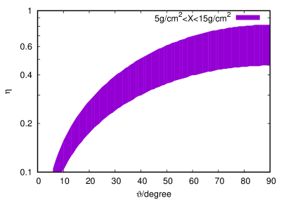
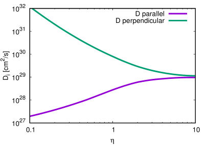
Figure 7: Left panel: Grammage $X$ crossed by CRs in a “disc and halo” model, for the diffusion coefficients shown in the right panel of Fig. 6, as a function of the tilt angle $\vartheta$ between the regular magnetic field and the Galactic plane, and of the turbulence level $\eta$. Right panel: Fit of the diffusion coefficients $D_{\|}$ and $D_{\perp}$ from the right panel of Fig. 6 at $E=10^{15}$ eV as function of $\eta$.

As a result of the anisotropic CRs propagation, the diffusion coefficient perpendicular to the ordered field can be between two and three orders of magnitude smaller than the parallel one, $D_{\bot}\ll D_{||}$, as shown in the right panel of Fig. 7. Then the $z$ component of the regular magnetic field can drive CRs efficiently out of the Galactic disk. For instance, the “X-field” in the Jansson-Farrar model [155] for the GMF leads to the correct CR escape time, if one chooses as turbulence level $\eta\simeq 0.25$ [156]. For this choice, the diffusion coefficients satisfy $D_{\|}\simeq 5D_{\rm iso}$ and $D_{\perp}\simeq D_{\rm iso}/500$, where $D_{\rm iso}$ denotes the isotropic diffusion coefficient $D_{\rm iso}$ satisfying the B/C constraints. In the regime, where the CRs emitted by a single source fill a Gaussian with volume $V(t)=\pi^{3/2}D_{\perp}D_{\|}^{1/2}t^{3/2}$, the CR density is increased by a factor $500/\sqrt{5}\simeq 200$ in the case of anisotropic diffusion. The smaller volume occupied by CRs from each single source leads to a smaller number of sources contributing substantially to the local flux, with only $\sim 10^{2}$ sources at ${\cal R}\sim 10$ GV and about $\sim 10$ most recent SNe in the TeV range. This reduction of the effective number of sources may invalidate the assumption of continuous CR injection and a stationary CR flux.

Impact of the Local Bubble

Another challenge for the simple diffusion picture with a constant diffusion coefficient throughout the Milky Way is the observation that the Sun resides inside the Local Bubble. This implies, e.g., the question how biased local measurements are. Surprisingly, the impact of the Local Bubble on the propagation of CRs has been largely neglected so far. An exception is, e.g., Ref. [157], where the influence of a local under-density on the propagation of radioactive isotopes was examined using a two-zone diffusion model. However, this work assumed that no sources reside inside the Local Bubble—in contrast to the picture that the bubble was created by recent SN explosions. In Ref. [158], it was suggested that the locally measured spectra of primary nuclei contain at low energies a component which was accelerated in the Local Bubble. The presence of this additional component allowed the authors to explain both the antiproton flux in the GeV range and B/C ratio without using artificial breaks in the diffusion coefficient and the primary injection spectrum. In Ref. [159], it was speculated that the knee may be caused by the fast escape of CRs generated inside the bubble above 4 PeV. The more recent studies [160, 161, 154] suggest that the effects of the Local Bubble can be profound, changing in particular strongly the contribution from recent nearby CR sources as Vela to the locally observed CR flux.

2.3 Observations and anomalies

2.3.1 Anisotropy of cosmic rays up to the knee

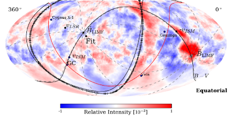
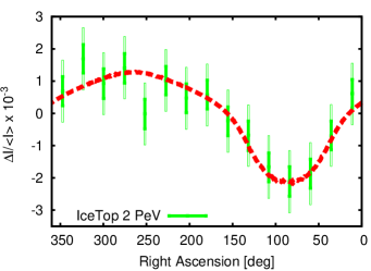
Figure 8: Left panel: All-sky map of the CR intensity combining HAWC and IceCube data at 10 TeV median energy after subtracting multipoles with $\ell\leq 3$. The magnetic equator as the plane containing the magnetic field in the local ISM [162] is shown as a black curve, the Galactic plane as a red curve and the positions of two nearby SNR, Geminga and Vela, are indicated too; adapted from Ref. [163]. Right panel: The relative intensity projected on the equatorial plane as function of right ascension at 2 PeV, adapted from Ref. [164].

The observed intensity of CRs is characterised by a large degree of isotropy up to the highest energies. This indicates that turbulent magnetic fields inside the Milky Way are able to isotropize the Galactic part of the CR flux at least up to knee. A CR dipole anisotropy at the level of $10^{-3}$ was measured above 100 GeV starting from the 1970s. However, only recently an almost all-sky coverage was reached at multi-TeV energies combining HAWC data from the northern and IceCube data from the souther hemisphere [163]. In addition to the expected dipole anisotropy and other large-scale anisotropies reflecting the non-uniformity of the CR source distribution, higher multipoles have been detected which are visible by eye in the map shown in the left panel of Fig. 8. These small-scale anisotropies are most likely connected to the local structure of the turbulent GMF and the heliosphere; for a detailed discussion see Refs. [165, 166]. Additionally, the shape of the anisotropy shown in the right panel which deviates from the cosine shape expected for a pure dipole contains useful information about the type of magnetic field fluctuations on which CRs scatter [164]. Here we consider only the dipole component of the anisotropy.

The magnitude of the dipole anisotropy $\boldsymbol{\delta}$ of the CR intensity $I=c/(4\pi)n$ is defined by

$$\delta\equiv\frac{I_{\max}-I_{\min}}{I_{\max}+I_{\min}}.$$ (18)

In most cases, CR experiments measure only the projection of the dipole vector on the equatorial plane. This implies in particular that the measured magnitude is smaller than the true one, except $\boldsymbol{\delta}$ would be contained in the equatorial plane. Moreover, only the phase, i.e. the right ascension of the projected dipole vector, is experimentally determined.

The (projected) dipole anisotropy $\delta$ measured by seven experiments is shown in Fig. 9 as function of energy. The phase of the anisotropy shown in the left panel is close to constant up to 200 TeV, flips then by approximately $180^{\circ}$ and stays again constant up to 100 PeV. At even higher energies, the phase changes smoothly. The amplitude of the dipole anisotropy shown in the right panel changes rather smoothly at low energies, being first approximately constant followed by a decrease in the range between 10–200 TeV. This decrease stops abruptly at 200 TeV, i.e. at the same energy where the phase flips by $180^{\circ}$. Above 10 PeV, only limits by KASCADE-Grande and PAO exist up to the energy $E>8$ EeV, where the dipole is again detected.

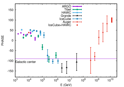
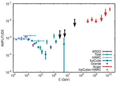
Figure 9: The dipole component of the CR anisotropy as function of energy as measured by ARGO [167], Tibet [168, 169], HAWC [170], IceCube [171], combining HAWC and IceCube [172], KASCADE-Grande [173] and the PAO [174]: the phase (left panel) and the amplitude (right panel) as function of energy.

The behaviour of the dipole anisotropy $\delta$ as function of energy up to 200 TeV seems at first sight difficult to reconcile with diffusive CR propagation: In this picture, CRs are most efficiently scattered by those turbulent field modes which wave-length equals their Larmor radius. Therefore the scattering rate is energy dependent and determined by the fluctuation spectrum of the turbulent GMF. As result, both the diffusion coefficient and the CR anisotropy are expected to increase with energy with the same rate. Thus the decrease of the CR anisotropy appears to be in contradiction to Kolmogorov-like diffusion which is supported, e.g., by the AMS-02 result on the B/C ratio [127]. Moreover, the abrupt change of the dipole phase is difficult to explain in the simplest diffusion approach where the dipole is aligned with the CR flux, $\boldsymbol{j}\propto\boldsymbol{\nabla}n$. In this picture, only small variations of the dipole direction are expected, if the CR sea is smooth and many sources contribute. Finally, it has been often stressed that the observed amplitude of the dipole anisotropy is small compared to the theoretical expectation [175, 176]. These discrepancies were dubbed the “CR anisotropy problem” by Hillas [175].

2.3.2 Primary cosmic ray nuclei

The energy spectra of primary CRs measured by direct detection experiments, i.e. up to energies $E\simeq 10^{14}$ eV, were until 2010 well described by a featureless power law with slope $\alpha\simeq 2.7$. The absence of structures indicates that a common acceleration mechanism in CR sources is at work and that features connected to the age or maximal energy of individual sources are averaged out, because a large number of sources contributes to the locally observed CR flux. In other words, a “sea” of Galactic CRs exists at these energies, which is well mixed. As a consequence, the energy spectra of primary cosmic rays should be also universal, being, e.g., independent of the Galactic longitude. Moreover, CR spectra expressed as function of rigidity should not depend on the type of nuclei as long as interactions can be neglected. However, the idea of a perfectly mixed CR sea is an approximation, and thus deviations from this picture should appear as soon the experimental sensitivity is sufficiently improved.

Breaks in the rigidity spectrum

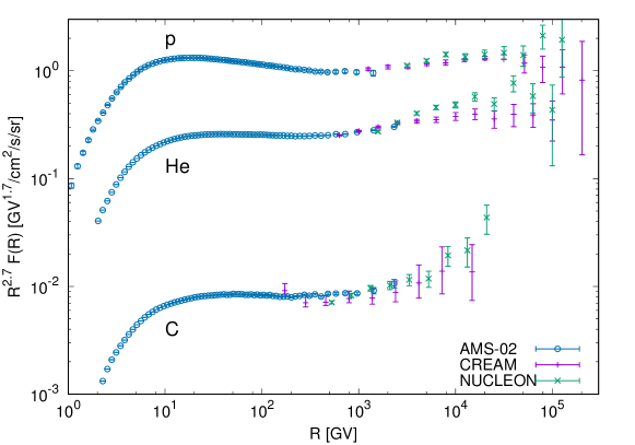
Figure 10: The spectrum of proton, helium and carbon as function of rigidity, measured by the AMS-02 [126, 177], CREAM [178] and NUCLEON experiments [179, 180].

In 2010, the CREAM collaboration announced results from two balloon flights for the spectra of CR nuclei with energies between 2.5 TeV and 250 TeV [181]. Compared to the extrapolation of data at lower energies, the proton and helium spectra measured were much flatter, with the helium flux $4\sigma$ higher than expected. Similar results were obtained for the fluxes of heavier nuclei, which were all consistent with a break around 200 GeV/n. These results were later confirmed by the PAMELA [182], Fermi-LAT [183] and AMS-02 experiments [126, 184]. A summary of recent measurements is shown in Fig. 10 for the spectra of protons, helium and carbon nuclei. The best-fit obtained by the AMS-02 collaboration to the proton flux between 45 GV and 1.8 TV using a broken power law has its break at $336^{+68}_{-44}$ GV where the slope changes from $\alpha=2.85$ to $\alpha=2.72$ [126]. For helium, a fit of the flux between 45 GV and 3 TV gave a break at $245^{+35}_{-31}$ GV, where the slope changes from $\alpha=2.78$ to $\alpha=2.66$. At higher energies, there are indications for additional features in the energy spectrum. The new space experiment NUCLEON measured a knee-like feature at $R=10$ TV with $3\sigma$ significance in its first two years of observations  [185]. This result still needs confirmation with better statistics. In Fig. 10, one can see, that the results of both the CREAM and the NUCLEON experiments are consistent with AMS-02 in their common energy range, but their results are somewhat differ at higher energies.

Deviation from rigidity dependent power laws

If the breaks in the CR nuclei spectra discussed above are caused by acceleration or propagation effects, the rigidity spectra of different nuclei should have the same shape and differ only in their normalisation. However, already the first CREAM results in 2010 provided strong evidence that the spectra of proton and helium differ above the break. Recall also from Fig. 3 that interactions do not influence the proton and helium spectra even at the lowest energies. The findings of CREAM were confirmed by the AMS-02 experiment which found a clear change in the ratio of the proton and He fluxes [184], cf. with Fig. 10: Their results indicate that the spectral index $\gamma_{\rm p/He}$ of the p/He flux ratio increases with rigidity up to 45 GV and becomes then constant, $\gamma_{\rm p/He}=-0.077\pm 0.02$ [184]. As a result of the harder helium spectrum, the proton and He flux are crossing over in the energy range 3–10 TeV.

Gamma-ray observations

Since the locally measured CR spectrum is up to $\sim 30$ GV affected by the Solar wind, indirect measurements of the CR flux using gamma-rays are a valuable alternative. In this case, one uses the knowledge of the differential hadronic production cross section of photons to infer the shape of the primary CR flux. At very low energies, a possible contribution of electron Bremsstrahlung or changes of CR propagation inside dense molecular clouds has to be taken into account.

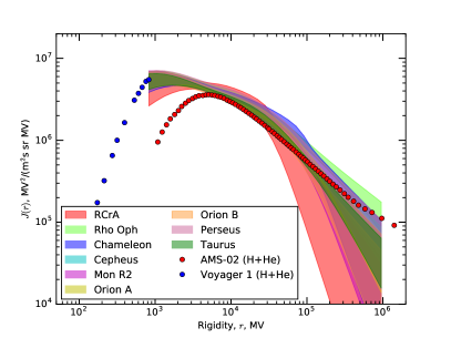
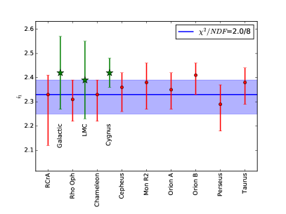
Figure 11: Proton plus helium spectrum of individual molecular clouds as function of rigidity (left) and the corresponding exponent of the power law below the break (right); from Ref. [186].

One possibility to perform such an indirect determination of the CR flux is to use the gamma-ray flux measured by the Fermi-LAT experiment from giant molecular clouds in the Gould belt, which is located at the distance 200–500 pc from us. Using the first years of Fermi data, Ref. [187] concluded that the measured gamma-ray spectrum can not be fitted with a single power law for the CR spectrum, but requires a break around $E\simeq 9$ GeV. The claim of such a break was initially disputed [188, 189], but became stronger with larger statistics. The most recent analysis using almost 10 years of data had enough events to study individual clouds separately [186]. In the left panel of Fig. 11, the derived CR spectra of individual clouds as function of rigidity are shown. The spectra from all molecular clouds are fitted with a broken power law and are normalized to the Voyager 1 data at low energies. In the right panel, the indices of the power law below the break determined for individual clouds are compared to the one of the central part of the Milky Way, the Large Magellanic Cloud, and the Cygnus region. One can see that the molecular cloud spectra below the break are consistent with the spectral index $\alpha=2.3\pm 0.1$. These values are also consistent with the spectrum from the central Galaxy and from the Large Magellanic Cloud, but deviate from the locally observed slope $\alpha\simeq 2.7$. In contrast to the spectrum below the break, both the position of the break and the slope after the break differ in individual clouds [186].

Gamma-ray observations can be also used to compare the CR spectrum as function of Galactic longitude. In Ref. [190], the spectral slope in the central Galaxy was determined as $\alpha\simeq 2.4$ compared to the steeper $\alpha\simeq 2.7$ found from local measurements. In the more detailed study of Ref. [191], it was then shown that the slope of the CR spectrum strongly depends on the Galactic longitude: Considering only the Galactic plane, $|b|\leq 5^{\circ}$, the slope varies between $\alpha\simeq 2.5$ towards the Galactic center and $\alpha\simeq 2.8$ in the outer Galaxy. Note, however, that these results were challenged recently by Ref. [192] which finds a rather homogeneous CR sea below 100 GeV.

2.3.3 Primary electrons

The flux of CR electrons has been measured recently by several experiments. While the magnetic spectrometers PAMELA and AMS-02 can separate electrons and positrons, other experiments like H.E.S.S., Fermi-LAT, DAMPE, and CALET perform calorimetric measurements of the sum of electrons and positrons. In the left panel of Fig. 12, we show the combined electron plus positron flux $F(E)$ multiplied with $E^{3}$ measured by AMS-02 [193], Fermi-LAT [194], H.E.S.S. [195], DAMPE [196], and CALET [197]. The spectrum $E^{3}F(E)$ has a peak at 10 GeV and is affected by solar modulations at energies $E\raise 1.29167pt\hbox{$\;<$\kern-7.5pt\raise-4.73611pt\hbox{$\sim\;$}}20$ GeV, as one can see from the differences between the data of PAMELA and AMS-02 which measured the electron flux at different times, for more details see Ref. [198]. Between 20 and 50 GeV, the spectrum hardens gradually and is then up to $\simeq 500$ GeV well described by a power law with spectral index $\alpha_{\rm e^{-}}\simeq 3.17$. Finally, the combined electron plus positron flux has a strong break at 1 TeV, as it was first shown by data from H.E.S.S. The shape of this break and the suppression measured by the different experiments vary, indicating underestimated systematic errors. From the measurement of the positron flux (discussed later and shown in Fig. 15), one can estimate a flux ratio of positron-to-electrons $\raise 1.29167pt\hbox{$\;<$\kern-7.5pt\raise-4.73611pt\hbox{$\sim\;$}}10\%$ at 1 TeV. Thus the break in the combined electron plus positron flux at 1 TeV is a break in the electron flux. The data, in particular of H.E.S.S., above the break are consistent with a new, steeper power-law.

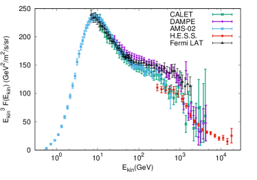
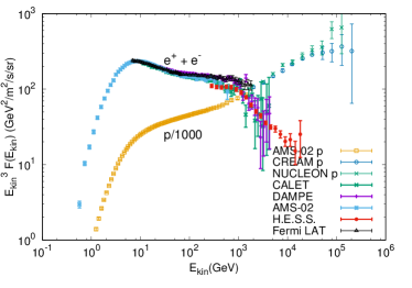
Figure 12: Left panel: Cosmic ray electron plus positron energy spectrum measured by AMS-02 [193], Fermi-LAT [194], H.E.S.S. [195], DAMPE [196], and CALET [197]. Right panel: Comparison of the proton spectrum from Fig. 10 (divided by 1000) and the electron plus positron spectrum.

In the right panel of Fig. 12, we compare the proton and electron (plus positron) spectra. The two spectra have different slopes and normalisations of the power law. The difference in normalisation is caused by the different injection mechanism into the acceleration process for electrons and protons, while the steeper slope of electrons should be caused by their energy losses. In the diffusion picture, the energy losses of electrons should lead to two cooling breaks in the observed flux of electrons [33]. A first break, where the slope changes from $F(E)\propto Q(E)\propto E^{-\alpha}$ to $F(E)\propto E^{-(\alpha+1/2)}$ is expected at the energy when the average path length of electrons becomes comparable to the height $H$ of the CR halo. A second break with a steepening to $F(E)\propto E^{-(\alpha+1)}$ should occur, when the average path length becomes comparable to the height $h$ of the thin disk containing CR sources. Combining the distance $d\simeq\sqrt{2D\tau_{1/2}}\simeq\sqrt{2D/(bE)}$ an electron diffuses during its energy loss time (cf. with Eq. (6)), we can estimate the energy of the first break: Assuming $H=5$ kpc, Kolmogorov diffusion with $D_{0}=5\times 10^{28}$cm²/s at $E_{0}=10$ GeV and $b=1.4\times 10^{-16}({\rm GeV\,s})^{-1}$, it follows $E_{1/2}\sim 1$ GeV. Thus the break is hidden in the energy region where solar modulations strongly modify the shape of the electron flux. At higher energies, say above 30 GeV, one expects thus the slope $\alpha\simeq 2.85+0.5=3.35$ for the electron flux. The second break with a steepening to $\alpha\simeq 3.85$ is expected at 10–100 TeV. This simple picture is in clear contradiction to the energy dependence of the measured flux. In particular, the gradual hardening of the spectrum between 20 and 50 GeV is difficult to explain as the contribution from an uniform background of electron sources. If the hardening would be a propagation effect, some imprint should be also seen at the same energy range in the proton spectrum which is shown in the right panel of Fig. 12. However, the hardening in the proton spectrum happens at a higher energy and is less pronounced. A possible explanation to both features is the appearance of a new component in the CR flux: Such a new contribution is expected to dominate the steeply falling electron spectrum at lower energies than the proton spectrum.

2.3.4 Secondary nuclei

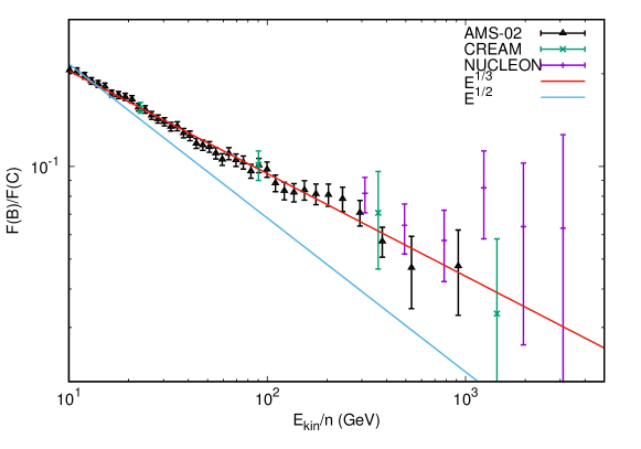
Figure 13: Boron-to-carbon ratio as function of kinetic energy per nucleon measured by the CREAM [199], AMS-02 [127], and NUCLEON [200] experiments. The power law predicted by Kolmogorov turbulence ($1/E^{1/3}$) and Iroshnikov-Kraichnan turbulence ($1/E^{1/2}$) at high energies are also shown.

In the diffusion picture, the fluxes of light primary CRs given by Eq. (9) are connected by $n_{p}=Q_{p}\tau_{\rm esc}\propto Q_{0}E^{-(\alpha+\delta)}$ to the slopes $\alpha$ and $\delta$ of the injection spectrum and the diffusion coefficient, respectively. Combining the locally observed $1/E^{2.7}$ spectrum with the prediction from diffusive shock acceleration, $\alpha=2.0-2.2$, suggests therefore $\delta=0.5$ corresponding to Iroshnikov-Kraichnan turbulence. On the other hand, $\delta=0.5$ leads to a fast increase of the CR dipole anisotropy, in contradiction to the behavior of $\delta$ as function of energy shown in Fig. 9.

The value of $\delta$ can be determined from secondary-to-primary ratios like B/C which scale as ${\cal R}^{-\delta}$, if $X_{\rm esc}/X^{(B)}\ll 1$, cf. with Eq. (12). From Fig. 3, we see that the latter condition is satisfied at ${\cal R}\gg 30$ GV. In Fig. 13, we show the B/C ratio as function of the kinetic energy per nucleon measured by the AMS-02 [127], CREAM [199] and NUCLEON [200] experiments. One can see that the data are consistent with the slope $\delta=1/3$ predicted by Kolmogorov turbulence, while the decrease of the B/C ratio predicted by Iroshnikov-Kraichnan turbulence is too strong. The data above $E_{\rm kin}/n\raise 1.29167pt\hbox{$\;>$\kern-7.5pt\raise-4.73611pt\hbox{$\sim\;$}}500$ GeV hint for a flattening of the B/C ratio at high energies, but the large errorbars prevent any firm conclusion.

Taken at face value, the observation that the boron-to-carbon ratio follows Kolmogorov turbulence has important consequences: It implies that either the acceleration spectrum of Galactic CR sources is softer than expected, being close to $1/E^{2.4}$. Such soft spectra would compound the problem of reaching sufficiently high maximal energies in Galactic CR sources. Or the simple diffusion picture which was used in our argument has to be modified. For instance, models which invoke strong advection can reproduce the B/C data using Iroshnikov-Kraichnan turbulence. Alternatively, the locally observed CR spectra may deviate from the global average. Such a deviation may be expected if the number of CR sources is relatively small.

2.3.5 Radioactive isotopes

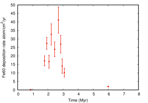
Figure 14: Deposition rate of ⁶⁰Fe in the ocean crust as function of time from Ref. [201].

The average time $\tau_{\rm esc}$ CRs spent in the Milky Way before escape can be deduced from the suppression, due to radioactive decay, of the flux of unstable nuclei that have a lifetime comparable with their residence time in the Galaxy. Comparing the fluxes of two isotopes of the same chemical element, one stable and the other unstable, allows one to measure this suppression, what in turn can be used to estimate $\tau_{\rm esc}$. Beryllium is a very rare element in ordinary matter, and essentially all beryllium nuclei in CRs are secondaries formed by the fragmentation of heavier nuclei, cf. with Fig. 2. It has two stable isotopes ( ⁹Be, and ⁷Be, if it is fully ionized) and one unstable (¹⁰Be) with the half-life $\tau=(1.51\pm 0.04)$ Myr. The CRIS collaboration used a leaky-box model to convert their measurements of the beryllium ratio ${}^{10}{\rm Be}/(^{7}{\rm Be}+^{9}{\rm Be})$ in three different bins of kinetic energy around 100 MeV/nucleon into the estimate $\tau_{\rm esc}=(15.0\pm 1.6)$ Myr for the escape time [202].

In 1996, it was suggested that rare, long-lived radioactive isotopes can be used as probes of nearby SN explosions [203]. Such isotopes as ⁶⁰Fe with a half-lifetime of $2.6$ Myr [204] can be searched for in sediments on the bottom of oceans. The age of the ocean crust can be determined with ¹⁰Be dating. The first successful measurement was carried out in 1999, finding an enhanced ⁶⁰Fe concentration in a ferromanganese crust in the Southern Pacific [205]. This observation was confirmed using marine sediments at other locations [206, 207, 201] and the Moon [208]. In Fig.  14, we show results for the abundance of ⁶⁰Fe in the Earth crust from Ref. [201]. The peak in the ⁶⁰Fe abundance points to a SN event in the vicinity of the Earth $\simeq(2-3)$ Myr ago. The study of Ref. [209] suggested that more than one SN contributed to this peak. Modelling the transport of dust grains containing ⁶⁰Fe, Ref. [210] suggested a distance of order 100 pc to the SNe. For a review and discussion of other radioactive elements than ⁶⁰Fe see Refs. [211, 212].

2.3.6 Secondary positrons and antiprotons

Positrons and antiprotons are produced as secondaries by CR protons and nuclei in the interactions with interstellar gas. While positrons also can be produced as primaries in pulsars through $e^{+}e^{-}$ pair production, astrophysical sources of primary antiprotons do not exist, offering an opportunity to search for new phenomena and exotic physics. Similarly to the case of secondary nuclei, the decrease of the escape time $\tau_{\rm esc}=\tau_{0}(E/E_{0})^{-\delta}$ with energy should soften the slope of the positrons and antiprotons secondaries relative the primary spectrum by $\delta=1/3$ in the case of Kolmogorov turbulence. For positrons, energy losses due to synchroton radiation and Thompson scattering on background photons result in an additional softening, as discussed for primary electrons. Thus the expectation in the standard diffusion picture is that both the positron-to-electron ratio $R_{e^{+}/e^{-}}$ and the antiproton-proton ratio $R_{\bar{p}/p}$ should decrease with energy.

In Fig. 15, we present in the left panel the AMS-02 positron flux from Ref. [213] as function of energy with red errorbars. Above $\simeq 30$ GeV, when the effect of solar modulations can be neglected, an ankle-like feature around 50 GeV and a break at 300 GeV are visible. This break in the positron spectrum happens at lower energy, and is much softer than the one in the electron spectrum. In the right panel, we show the corresponding positron-to-electron ratio $R_{e^{+}/e^{-}}$, which clearly deviates from the expectation for a pure secondary production. Additionally, we show in the left panel with black errorbars the antiproton flux measured by AMS-02 [214]. As it was noted in Refs. [215, 214, 216], a positron-to-antiproton flux ratio close to 2 is consistent with expectations that both are produced in hadronic interactions. To illustrate this fact, we also show the proton flux measured by AMS-02 [213] and CREAM [178], changing the normalisation by a factor $10^{-3}$. Additionally, we rescaled the energy of the proton flux by a factor 20 down, taking thereby into account that the energy transferred to positrons is around 5%. One can see, that below 50 GeV, the positron flux is much steeper than the proton flux, while above this energy up to the break around 300 GeV, the slopes of the two fluxes are similar. The antiproton flux above 50 GeV repeats the slope of the proton flux, but the relatively large errorbars at high energies prevent any definite conclusion on its high energy behaviour.

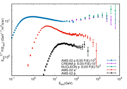
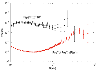
Figure 15: Left panel: Positron and antiproton spectra from the AMS-02 experiment [213, 214]. For comparison, we show the proton spectrum from Fig. 10, divided by $10^{3}$ and rescaled in energy $E/20$. Right panel: The positron-to-electron ratio $R_{e^{+}/e^{-}}$ from Ref. [217] and the antiproton-to-proton ratio $R_{\bar{p}/p}$ from Ref. [214].

While the positron-to-electron ratio $R_{e^{+}/e^{-}}$ shown in the right panel of Fig. 15 is clearly incompatible with pure secondary production of positrons, the larger errorbars both in theoretical predictions and the experimental flux determination make the situation for antiprotons less conclusive: For instance, Ref. [218] found no unambiguous evidence for a significant excess with respect to expectations. This conclusion requires however, that all uncertainties in the cross section and propagation model are by chance correlated, increasing thereby the prediction. Similarly, Ref. [219]. found an antiproton spectrum which is only slightly lower than the data combining a GALPROP diffusion model including advection and reacceleration for the interstellar and HelMod for the heliospheric propagation. Thus a conclusive statement that antiproton measurements require an additional source of antiprotons requires a reduction of the current errors, both in theoretical predictions and experimental measurements.

2.4 Models

We now review the main types of models suggested as explanation for the anomalies discussed in the previous section. First we discuss possible explanations of the observed behaviour of the CR anisotropy as function of energy, restricting ourselves to the the dipole part of the anisotropy and energies up to the transition to extragalactic CRs, $E\raise 1.29167pt\hbox{$\;<$\kern-7.5pt\raise-4.73611pt\hbox{$\sim\;$}}{\rm few}\times 10^{17}$ eV. Then we discuss models addressing the spectral features observed in the CR energy spectra, starting from models aiming to explain the anomalies in the secondary fluxes. After that, we review models for the breaks in the CR nuclei spectra, and finally models which try to to explain several features simultaneously.

2.4.1 Explaining the anisotropy

In the diffusion approximation, Fick’s law is valid and the net CR current $\boldsymbol{j}(E)$ is determined by the gradient of the differential CR number density $n(E)={\rm d}N/({\rm d}E{\rm d}V)$ and the diffusion tensor $D_{ij}(E)$ as $j_{i}=-D_{ij}\nabla_{j}n$. Then the dipole vector $\boldsymbol{\delta}$ of the CR intensity $I=c/(4\pi)n$ follows as

$$\delta_{i}=\frac{3}{c}\frac{j_{i}}{n}=-\frac{3D_{ij}}{c}\frac{\nabla_{j}n}{n}\,.$$ (19)

If the ordered magnetic field $\boldsymbol{B}$ dominates, the tensor structure of the diffusion tensor simplifies,

$$D_{ij}=D_{\|}e_{i}e_{j}+D_{\perp}(\delta_{ij}-e_{i}e_{j})+D_{A}\varepsilon_{ijk}e_{k}\simeq D_{\|}e_{i}e_{j},$$ (20)

except for observers which are nearly perpendicular to the magnetic field line through the source. Here, $\boldsymbol{e}$ is a unit vector in the direction of the ordered magnetic field, while the diagonal elements of the diffusion tensor describe diffusion along ($D_{\parallel}$) and perpendicular ($D_{\perp}$) to the ordered field. The off-diagonal antisymmetric component ($D_{\rm A}$) appears only, if drift terms for CRs are included. Thus in the limit of a strong ordered field, $D_{ij}\simeq D_{\|}e_{i}e_{j}$, the CR gradient is projected onto the magnetic field direction [220]. Therefore anisotropic diffusion predicts that the dipole anisotropy should align with the local ordered magnetic field instead of pointing to the source [220, 221]. Note that the ordered magnetic field corresponds to the sum of the regular magnetic field and the sum of turbulent field modes with wavelengths larger than the Larmor radius at the corresponding CR energy. This implies that CRs with $R_{\rm L}\ll L_{\rm c}$ propagate anisotropically even in the absence of a regular magnetic field, since the field modes with $k/(2\pi)\gg R_{\rm L}$ act locally as an ordered field [94].

In the case of a (three-dimensional) Gaussian CR density $n$, the formula (19) can be evaluated analytically. The result $\delta=3R/(2cT)$ for a single source with age $T$ and distance $R$ is independent of the regular and turbulent magnetic field. In Ref. [221], it was shown that the CR density of a single source is quasi-Gaussian, if CRs propagate over length scales $l\gg L_{\rm coh}$. This implies in particular that there is no “mis-alignment effect” which can reduce the absolute value of the dipole anisotropy: For instance, an observer perpendicular to the magnetic field line through the source will pick up $D_{\perp}\nabla_{\perp}n$ in Eq. (19). But since $D_{\perp}$ will be cancelled taking the derivative, its small value has no influence on the anisotropy. Numerically, the dipole anisotropy $\delta$ of a source contributing the fraction $f_{i}$ to the total observed CR flux is thus

$$\delta_{i}=f_{i}\,\frac{3R}{2cT}\simeq 5.0\times 10^{-4}\>f_{i}\,\left(\frac{R}{200\,{\rm pc}}\right)\left(\frac{T}{2\,{\rm Myr}}\right)^{-1}\,.$$ (21)

The plateau in the range 2–200 TeV visible in the experimental data for the dipole anisotropy shown in Fig. 9 is naturally explained by the energy-independent contribution to the dipole anisotropy of a single source. This is supported by the fact that the dipole phase remains approximately constant in this range too, before it flips by $\sim 180^{\circ}$. Such a flip is naturally explained by the projection effect on the magnetic field line, if above 200 TeV another source, which is located in the opposite hemisphere, dominates the CR dipole anisotropy.

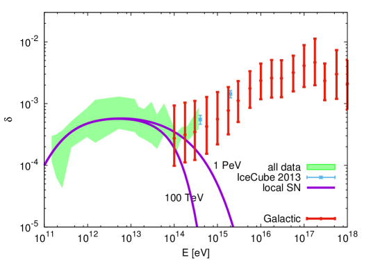
Figure 16: Lower and upper limit (green band) on the dipole anisotropy and data from IceCube (blue errorbars) compared to the contribution from the local source (magenta, for two values of $E_{\max}$) and from all Galactic SNe (red) calculated in the escape model of Ref. [156, 222].

More specifically, it was suggested in Ref. [221] that a 2–3 Myr old source at the distance 200–300 pc dominates the dipole anisotropy in the range 2–200 TeV. The contribution of this local source is shown in Fig. 16 by two magenta lines for two different high-energy cutoffs: In one case, it was assumed that the source can accelerate up to 100 TeV, in the other that it is a PeVatron. In both cases, the CR flux was calculated following the trajectories of individual CRs, as discussed in Refs. [156, 222, 215, 223]. Additionally, the total anisotropy beyond $10^{14}$ eV of all Galactic SNe is shown by red error-bars which was calculated in the escape model which uses the same magnetic field configuration as the one used for the loal source [156, 222].

A characteristic feature of this proposal is that a relatively old source dominates the observed CR flux. This is only possible in the case of anisotropic diffusion, and requires additionally that the perpendicular distance $d_{\perp}$ of the Sun to the magnetic field line connecting it to the source is not too large. Even for small $d_{\perp}$, the CR flux from the single source is suppressed at low-energies, because of the slower perpendicular diffusion. In Ref. [223], the value $d_{\perp}\simeq 70$ pc was estimated requiring that the low-energy break in the source spectrum explains the breaks in the energy spectra of CR nuclei. For this choice of $d_{\perp}$, the flux of the local source is suppressed below $\simeq 1$ TeV (cf. with Fig. 2 of Ref. [223]), leading to a decreasing $f_{i}$ and the transition to the standard $\delta\propto E^{1/3}$ behavior below this energy.

Another choice for the age of the source was suggested in Refs. [224, 225]. Here, Vela with the age around 11,000 yr and distance 300 pc was proposed as the single source responsible for the observed plateau in the dipole anisotropy. In this case, the contribution of Vela to the dipole amplitude has to be suppressed by a factor $\simeq 200$. Three mechanisms for such a suppression may be operating: First, if the regular magnetic field and the CR gradient are not parallel, the projection effect in $D_{ij}\nabla_{j}n$ can reduce the dipole [226, 225]. Second, the measured CR dipole is a projection into the equatorial plane and is thus reduced compared to the true one. Finally, the CR flux contributed by Vela may be small. Calculating the CR fluxes from nearby young sources using the standard isotropic diffusion coefficient and taking into account these effects, Ref. [225] argued that Vela leads to the correct level of anisotropy. There are however two caveats in this conclusion: First, we recall that the projection effect in $D_{ij}\nabla_{j}n$ does not change the dipole amplitude, if the CR density is quasi-Gaussian [221]. Second we note that Ref. [225] calculated the CR fluxes from individual sources for isotropic diffusion. This requires that the regular magnetic field is weak enough, $\eta\raise 1.29167pt\hbox{$\;>$\kern-7.5pt\raise-4.73611pt\hbox{$\sim\;$}}5$, so that $D_{\perp}\simeq D_{\|}\simeq D_{\rm iso}$. Otherwise, a calculation of the CR flux following the lines of Refs. [221, 215, 223] would be required.

Finally, we note that none of these works took into account that the Sun resides inside the Local Bubble: As we discussed in section 2.1, the strength and the structure of the magnetic field in the bubble wall and the bubble interior is changed relative to the surrounding. Thus both the magnitude and the direction of the dipole amplitude may be changed compared to the predicition of Eq. (21).

2.4.2 Explaining secondaries

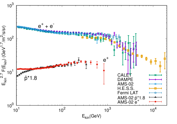
Figure 17: Positron and antiproton fluxes measured by AMS-02 [213, 214] compared to the electron plus positron flux. The antiproton flux is multiplied by the factor 1.8 expected for hadronic secondary production. The experimental data for the electron plus positron fluxes are the same as in Fig. 12.

Before reviewing the different classes of explanations for the excess of secondaries compared to the expectation in the standard diffusion picture, we want to stress a peculiarity of the observed flux ratios: The positron and antiproton fluxes above 100 GeV repeat the spectral shape of the proton flux, see Fig. 15. In contrast, the electron flux is considerably steeper than the positron and antiproton fluxes, as seen in Fig. 17. From Fig. 17, we can observe that the break of the positron flux at 300 GeV does not coincide with the break in the electron plus positron flux at 1 TeV. Moreover, the positron contribution to the combined electron plus positron flux is small. Therefore the slopes and breaks in the primary electron flux are unrelated to those in the positron flux.

The nearly scale invariance of hadronic interactions implies that the secondary fluxes produced in interactions of CRs on interstellar gas have a shape similar to the primary flux, if the grammage CRs cross is energy independent. Such an energy independence of the grammage is achieved, e.g., if a relatively young source contributes significantly to the observed local CR flux. Moreover, the ratio $R(E)=F_{e^{+}}(E)/F_{\bar{p}}(E)$ of the positron and antiproton fluxes is then mainly predicted by the properties of hadronic interactions, being proportional to the ratio of their $Z$ factors, $R=F_{e^{+}}/F_{\bar{p}}\propto Z_{e^{+}}/Z_{\bar{p}}\simeq 1.8$ [215, 216]. Such models predict also a corresponding increase of secondary nuclei like boron, which starts however at much higher rigidities.

The authors of Ref. [227] studied the secondary production of CRs avoiding the use of a specific model as far as possible. Assuming universal CR spectra, they derived the energy dependent grammage crossed by CRs from the B/C ratio measured by AMS-02. Then they used the grammage to derive the resulting antiproton flux as well as an upper bound on the positron flux. Their analysis supports a secondary origin of the positron and antiproton fluxes.

Pulsars

The most straightforward explanation for the observed rise of the positron-electron ratio $R_{e^{+}/e^{-}}$ assumes that primary sources of positrons exist. Pulsars are natural candidates for such primary positron sources, since electromagnetic pair cascades in their magnetospheres lead to a large positron fraction, $R_{e^{+}/e^{-}}\simeq 1$. In contrast, the antiproton flux would stay in this model on the level predicted in the standard difffusion picture, if the multiplicity of electron-positron pairs is large, as it is usually assumed for a cold MHD wind [228]. Since the energy losses of electrons increase fast with energy, the high-energy part of the $e^{+}+e^{-}$ spectrum should be dominated by local sources, as pointed out already 30 years ago [229, 230]. The expected electron and positron fluxes from pulsars, as well as the resulting anisotopy, have been studied in detail using the isotropic diffusion approximation [231, 232]. From the known pulsars, Geminga and PSR B0656+14 (which was thaught to be associated with the Monogem SNR) are the most promising candidates: They are located within 250–300 pc from the Sun and relatively young, $T=370$ kyr and $T=110$ kyr, respectively. For a pair-conversion efficiency around $\varepsilon_{e^{+}e^{-}}\sim 40\%$ and an injection slope $\beta\sim 1.5$–1.7, these two pulsars were found to give a reasonable fit to the PAMELA positron data and the total electron+positron flux measured by Fermi-LAT [231, 232]. The resulting anisotropy of the electron+positron flux peaks at $\sim 1$ TeV with $\delta\sim 1$%.

Recent HAWC observations of extended TeV gamma-ray emission from these two pulsars confirmed that they are local sources of accelerated electrons [233]. The spatial extension of the emission profile can be used to constrain the properties of the magnetic turbulent field in the region close to these sources. While the HAWC data are compatible with both isotropic Kolmogorov and Iroshnikov-Kraichnan turbulence, the absence of an asymmetry in the emission profile bounds the correlation length as $L_{\rm c}\raise 1.29167pt\hbox{$\;<$\kern-7.5pt\raise-4.73611pt\hbox{$\sim\;$}}5$ pc [234]. For the best-fit value of $B_{\rm rms}\simeq 3\mu$G for the strength of the turbulent field, the resulting diffusion coefficient at 100 TeV is $D\raise 1.29167pt\hbox{$\;<$\kern-7.5pt\raise-4.73611pt\hbox{$\sim\;$}}5\times 10^{27}$cm²/s. This value is compatible with those shown in Fig. 5, but much lower than the one required to reproduce, e.g., the observed B/C ratio. As a consequence of this slow diffusion, the HAWC collaboration concluded that the contribution of Geminga and PSR B0656+14 to the positron excess is negligble [233].

As we argued in Sec. 2.1, such a low value of the diffusion coefficient is connected to the absence of a strong regular field. Thus the hydrodynamic turbulence close to the source might have entangled the regular field, increasing the value of the turbulence level $\eta$. Alternatively, instabilities driven by escaping CRs could have increased $\eta$ [235, 236]. The possibility of strong magnetic field amplification is however disfavoured by the small value of $B_{\rm rms}\simeq 3\mu$G and the relatively small energy density of CRs compared to the ISM. In either case, the region with a reduced diffusion coefficient should be restricted to the close surrounding of the source. Thus two-zone diffusion models have been used to reevaluate the positron contribution of nearby pulsars, see e.g. Refs. [237, 238, 239]. Using a standard diffusion coefficient outside the sources, the positron flux is strongly increased relative to the analysis of Ref. [233] and can fit well the positron data. However, the presence of positrons with energies in the 10–1000 GeV range in the sources can be tested directly looking for GeV photons using Fermi-LAT. No GeV photon halo around Geminga and PSR B0656+14 has been found in the search performed in Ref. [240], and the derived upper limits were used to constrain their contribution to the observed positron flux as $\raise 1.29167pt\hbox{$\;<$\kern-7.5pt\raise-4.73611pt\hbox{$\sim\;$}}15\%$. The similar analysis [241] detected a weak GeV halo around Geminga and set an upper limit of $20\%$ to its contribution to the observed positron flux. These limits disfavour young pulsars as explanation for the positron excess. The question if the ensemble of old pulsars can explain the positron excess was studied in Ref. [242]. Scanning over a wide parameter space in pulsar properties and diffusion models, they identified cases in which the observed positron data can be reproduced. Successful models using Kolmogorov diffusion predict a positron fraction rising to $R_{e^{+}/e^{-}}\simeq 0.4$ at $\simeq 300$ GeV which flattens at higher energy—a behaviour which is in tension with the latest AMS-02 data.

Finally, we mention three alternative pulsar scenarios: In the first one, the contribution from the population of all millisecond pulsars was studied [243]. While pair cascades from the magnetospheres of isolated millisecond pulsars cut off around a few tens of GeV and thus cannot contribute to the high-energy rise of $R_{e^{+}/e^{-}}$, electron-positrons are accelerated up to tens of TeV in the strong intra-binary shocks of black widow and redback binary systems. In particular, Ref. [243] argued that the contribution to the positron flux by black widows and redbacks may reach levels of a few tens of percent at tens of TeV, depending on model parameters. A second alternative pulsar scenario was suggested recently in Ref. [244]: Using the low diffusion coefficient deduced from HAWC observations, an undecteted pulsar with age $\raise 1.29167pt\hbox{$\;<$\kern-7.5pt\raise-4.73611pt\hbox{$\sim\;$}}300.000$ yr inside the Local Bubble, i.e. at a distance of 30–80 pc, was proposed as explaination for the positron excess. This model predicts a rasing positron fraction $R_{e^{+}/e^{-}}$ reaching 25% at 1 TeV, which is disfavoured by the indication of a break at 300 GeV in the positron spectrum measured by AMS–02. A third alternative pulsar scenario are pulsar wind nebulae (PWN) with bow shocks [245, 246]. These shocks form, if PWNe move relative to the ambient ISM with supersonic speeds. Particles accelerated at the termination surface of the pulsar wind may undergo reacceleration in the converging flow formed by the outflow from the wind termination shock and the inflow from the bow shock, leading to a very hard energy spectra, $\beta\simeq 1.2$. For a conversion efficiency of $\eta\simeq 20\%$ of the pulsar spin-down energy into the acceleration of pairs and steepening of the spectrum at $E=500$ GeV to $\beta\simeq 2.3$, the measured positron fraction can be well reproduced.

Reacceleration in SNRs

Positrons produced by hadronic interactions in the vicinity of a SNR shock participate in the acceleration process and have therefore a flatter energy spectrum than primary electrons. In Ref. [247], it was suggested that the total spectrum of all positrons produced in a SNR is therefore flatter and that thereby the rise of the positron-electron ratio can be explained. Later, this scenario was applied to antiprotons [248] and secondary nuclei like boron or titanium nuclei [249]. All these works solved the diffusion equation in the stationary limit. Since therefore the number of produced secondaries is infinite, their production rates have to be normalised by hand: While the rate of positrons produced in the shock vicinity and thus taking part in the acceleration process is proportional to the time $t_{\max}$ acceleration is effective, the rate of positrons generated downstream is proportional to $D(E_{\max})/u^{2}_{1}$. Here, $D(E_{\max})$ is the diffusion coefficient at the maximal acceleration energy $E_{\max}$ and $u_{1}$ the advection velocity upstream. In general, these parameters are connected by the relation $D(E_{\max})/u^{2}_{1}\sim t_{\max}/20$ [23], and can therefore not be chosen arbitrarily. If however these parameters are treated as independent quantities, the relative size of the two components can be changed. Choosing them such that the reaccelerated component is enhanced, a raising secondary-to-primary ratio can be generated. Reference [247] argued that such a choice of parameters is motivated as an effective way to include the time evolution of the SNR. The boron-to-carbon ratio predicted in these reacceleration models for $R_{\max}=3$ TV is shown in the left panel of Fig. 18 [250]. For larger values of $R_{\max}$, the rise of B/C becomes more pronounced and evolves into a bump, while it disappears for $R_{\max}\raise 1.29167pt\hbox{$\;<$\kern-7.5pt\raise-4.73611pt\hbox{$\sim\;$}}1$ TV. In the right panel of Fig. 18, the positron flux predicted for $R_{\max}=3$ TV is shown.

In Refs. [251, 252], time dependent Monte Carlo simulations of the acceleration process and secondary production were performed. It was found that at any time, the reaccelerated and the downstream contributions to the secondary spectra add up approximately to a standard $1/E^{2}$ spectrum. This result suggests that the time dependence of parameters like the shock velocity or the magnetic field strength do not lead to an enhancement of secondary fluxes and, therefore, that reacceleration of secondaries in SNRs cannot explain the observed rising positron fraction. This conclusion is supported by the non-observation of a rise in other secondary ratios, as e.g. in B/C.

Supernovae in dense clouds

The authors of Refs. [253] suggested that a recent cluster of SN explosions happened in a nearby dense gas cloud. In this scenario, the cloud has been ionized by the ultraviolet radiation of OB stars. Then it is argued that particle acceleration continues in the radiative phase of the evolving SNRs, leading to a hard CR spectrum with slope $\alpha<2$ [254]. Protons interacting with the dense gas inside the cloud produce secondaries until the cloud is destroyed. Then both the primary CRs and the produced secondaries are released.

In the subsequent work [255], the same authors adapted the parameters of their model using now as slope of the CR spectrum $\beta=2.15$ and as injected energy in CRs $E_{\rm CR}=3\times 10^{50}$ erg. Moreover, they assumed a gas cloud with density $n\sim 50$/cm³ at the distance 100–200 pc. Particles were released $5\times 10^{5}$ yr ago, and diffuse afterwards isotropically with $\delta=0.4-0.6$. For these values, the resulting flux of secondaries can explain the rising positron fraction and leads also to an increase of the antiproton flux [255]. The results of this model are compared in Fig. 18 to the positron flux measured by AMS-02. The model predicts a rather sharp cutoff in the positron flux, since the positron production stopped $5\times 10^{5}$ yr ago. Therefore synchrotron cooling leads to a cutoff at $E\sim$ TeV in the positron spectrum. In contrast, the AMS-02 data indicate a break at $\sim 300$ GeV, suggesting the continuous injection of positrons from one (or several) older sources.

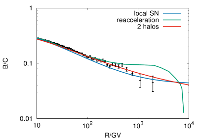
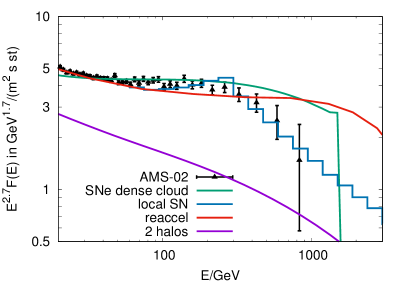
Figure 18: Left panel: Boron-to-carbon ratio as function of rigidity predicted in the reacceleration model [250] for $R_{\max}=3\times 10^{3}$ GV in the two-halo model from Ref. [256], and from a local SN [223]. Right panel: The positron flux in the reacceleration model from Ref. [250] for $R_{\max}=3\times 10^{3}$ GV, from SNe in a dense cloud [255], in the two-halo model from Ref. [256], and from a local SN [223].

Short CR confinement time

In Ref. [216], it was stressed that the ratio $R=F_{e^{+}}/F_{\bar{p}}\propto Z_{e^{+}}/Z_{\bar{p}}\simeq 1.8$ suggests that hadronic secondary production is the main source of these antiparticles. In a detailed study of how the softening feature induced by the energy losses emerges in the electron and positron spectra, two possibilities and their consequences were outlined [198]: In the traditional view discussed in Section 2.3.3, the softening break in the electron and the positron spectrum appears at the energy $\sim 1$ GeV. The alternative option advocated in Ref. [198] identifies the break in the electron flux at $\simeq 1$ TeV seen by the H.E.S.S. collaboration as the softening caused by the energy losses of electrons. This implies a much smaller confinement time of CRs, around 1 Myr at a few GeV. Since the confinement time is smaller than in the standard scenario, the diffusion coefficient is accordingly increased. As a result, the number of CR sources contributing to the locally observed flux is larger than usually. Another important prediction of this scenario are equal propagation properties of protons, electrons and their antiparticles below 1 TeV. In this scenario, the indications for a break in the positron spectrum at 300 GeV have to be therefore either wrong—or this break is caused not by energy losses, but is instead connected to spectral features of the positron sources.

2.4.3 Explaining the breaks and non-universal rigidity spectra

We review next models which explain the break at 300 GV in the CR nuclei spectra, the rigidity dependent p/He ratio and/or the longitude dependence of the CR spectrum.

Radial dependence of the turbulence

We discussed in section 2.3.2 that gamma-ray observations show evidence for a slope of the CR spectrum varying with Galactic longitude. In Refs. [257, 258], a gradual increase in the slope $\delta=\delta(R)$ of the CR diffusion coefficient with increasing distance $R$ from the Galactic centre was proposed. As a consequence, the CR flux and thus the resulting gamma-ray spectra are harder in the inner Galaxy. Combined with strong advection at $R<6.5$ kpc, the model could fit the CR proton flux, B/C and the diffuse gamma fluxes choosing $\delta(R)=aR+b$ with $a=0.035$ kpc^-1 and $b=0.21$. This model did not address the origin of the breaks in the CR spectra or the positron excess. It is however an example how Iroshnikov-Kraichnan diffusion, $\delta(R_{\odot})=0.5$, can be made compatible with the observed B/C ratio. Note also that a change in the slope $\delta$ of the CR diffusion coefficient implies a corresponding change in the power spectrum ${\cal P}(k)\propto k^{-\gamma}$ of the turbulent magnetic field, which are connected by $\gamma=2-\delta$. While it is natural that the normalisation of $D$ and ${\cal P}(k)$ changes towards the Galactic center, it is surprising that the type of turbulence depends on the Galactocentric distance $R$.

Two-halo models

In Ref. [256], it was suggested to divide the Galactic CR halo into two zones in which the rigidity dependence of the diffusion coefficient differ. In a version of this model updated after the release of the B/C data by AMS-02 [259], CRs diffuse slower than usually assumed, $D_{\rm i}({\cal R})\propto{\cal R}^{0.18}$, in an inner halo around the Galactic disk with the vertical extension $|z|<L_{\rm i}\simeq 0.5$ kpc. In contrast, CRs diffuse faster than usually in the outer halo, $D_{\rm o}({\cal R})\propto{\cal R}^{0.73}$, which has the extension $L_{\rm i}<|z|<L_{\rm o}$ with $L_{\rm o}\simeq 4$ kpc. The observed energy spectrum of primaries, which is usually given by $F(E)\propto Q(E)L/D(E)$, is then modified to

$$F(E)\propto\frac{Q(E)}{D_{\rm i}(E)/L_{\rm i}+D_{\rm o}(E)/L_{\rm o}}.$$

As a result, there are breaks in the slopes of primaries as well as in the secondary-to-primary ratios at high energies. This model describes successfully the hardening of the proton flux, but requires a different slope of the proton injection spectrum than that of other nuclei. Another prediction of this model is the decrease of the B/C ratio as $\propto{\cal R}^{-0.15}$ at high energies, cf. with Fig. 18. Moreover, it was speculated that the weak energy dependence $D_{\rm i}({\cal R})\propto{\cal R}^{0.15}$ may explain the plateau in the CR dipole anisotropy. While the positron flux is enhanced relative to standard diffusion models, the flux shown in the right panel of Fig. 18 falls short of the observed data. Therefore this model requires that pulsars generate the observed high-energy positron flux. Moreover, the antiproton flux is in this model in tension with the AMS-02 data, even if an additional antiproton component from interactions in CR sources is included [260].

Self-generated turbulence

The authors of Refs. [104, 105, 106] connected the breaks in the CR spectrum with a change in the energy dependence of the diffusion coefficient. In particular, they associated the break at 300 GV with the transition from self-generated CR turbulence to external turbulence injected by SN explosions and stellar winds associated with OB associations.

In such a model, the transport equation (4) of CRs is coupled to an evolution equation of plasma waves which describes the generation and damping of these modes,

$$\frac{\partial}{\partial k}\left[D_{kk}\frac{\partial W}{\partial k}\right]-\Gamma_{\rm CR}W=Q_{w}(k),$$ (22)

Here, $Q_{w}(k)$ is the generation rate of magnetic turbulence with wave-number $k$ by SNe and stellar winds, while $W(k)$ is the energy density of the magnetic turbulence normalised such that $B_{\rm rms}^{2}=B_{\rm tot}^{2}\int dk\,W(k)$. The turbulent cascade is determined by $D_{kk}=c_{k}|v_{A}|k^{7/2}W^{1/2}$ with the constant $c_{k}\sim 0.05$ [261]. Finally, $\Gamma_{\rm CR}$ is the rate by which CRs amplify the magnetic turbulence. In particular, a CR gradient along the $z$ direction will lead to a streaming instability with growth rate [262]

$$\Gamma_{\rm CR}=\frac{4\pi}{3}\frac{v_{A}}{kW(k)B_{\rm tot}^{2}}\left[p^{2}n(p)\right]_{p_{\rm res}},$$ (23)

with $p_{\rm res}$ denoting the CR momentum resonant with the turbulent field mode $k$. The streaming instability can lead to self-confinement of CRs, if its growth rate exceeds the rate of wave damping. Since less than 1% of the mass in the ISM is ionized, neutral-ion damping was considered first as the main damping mechanism. But despite the large mass fraction, partly ionized regions occupy only a small fraction of the volume of the ISM. Therefore ion-neutral friction prevents self-confinement of CRs even at low energies only inside cold clouds. In a fully ionized gas, nonlinear Landau damping where thermal ions Landau resonate with two turbulent wave modes is operative. Additionally, inhomogeneities in the ordered field lead to wave damping. In particular, the long-wavelength modes of the “standard” turbulence injected by SNe and stellar winds leads to a shearing of Alfvén waves, an effect which is however not well understood. As a result, the energy $E_{\ast}$ below which self-generated turbulence dominates can be only estimated, with $E_{\ast}\sim 100$ GeV as a typical value [263]. Note also that the variation in the CR density and the damping rate between, e.g., the Galactic disk and halo, should lead to a corresponding change in the value of $E_{\ast}$.

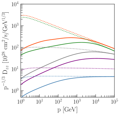
Figure 19: Left panel: Wave spectrum as a function of $k$ with (solid lines) and without (dashed lines) the contribution of self-generated waves at different $z$. Right panel: Diffusion coefficient as a function of momentum for different values of $z$; figures adapted from Ref. [101].

In the model of Refs. [104, 105, 106], the turbulent cascade introduces a scale $z_{0}\sim v_{A}L_{\max}^{2}/D_{kk}$ below which the turbulence is mainly self-generated. Effectively, this distance defines the boundary of the CR halo where CRs diffuse in Kolmogorov-like turbulence and an outer halo where CRs scatter on self-generated turbulence. Thus this model may be seen as physically motivated realisation of a two-halo model, although with quite different parameters. It reproduces the spectral break at rigidity $\simeq 300$ GV, but does not address the origin of the harder proton spectrum.

In Ref. [101], the coupled transport equation (4) for CR protons and the evolution equation (22) of plasma waves were generalised to include a dependence on the vertical distance $z$ to the Galactic disk and the advection of turbulence. In this way, a Galactic halo of CRs and self-generated magnetic turbulence was generated in a self-consistent way without introducing by hand a boundary for the CR halo. In the left panel of Fig. 19, the resulting wave spectrum at different distances $z$ to the Galactic disk is shown with (dashed lines) and without (solid lines) self-generated turbulence. The resulting diffusion coefficients shown in the right panel of Fig. 19 deviate for energies $\raise 1.29167pt\hbox{$\;<$\kern-7.5pt\raise-4.73611pt\hbox{$\sim\;$}}1$ TeV from the values for the Kolmogorov background turbulence. This implies that on scales smaller than $10^{-3}$ pc, the slope of the power spectrum of the turbulent magnetic field should deviate from $\gamma=5/3$. The proton spectrum obtained in this model reproduces well the experimental data from Voyager-1 up to the CREAM energy range.

Two-population models

This class of models explains the break at ${\cal R}\simeq 200$ GV as the transition between a source type dominating the low-rigidity and another type dominating the high-rigidity part of the spectrum. For instance, the authors of Ref. [144] proposed a three component model fitting the CR spectra between 10 GeV and 100 PeV. They suggested that the lowest energy component with ${\cal R}_{\max}=200$ GV is generated by novae, the intermediate component up to the knee with ${\cal R}_{\max}=4$ PV by isolated SNe, while the third component above the knee is generated by multiple SNe occurring inside of superbubbles.

In Refs. [264, 265], the hardening was connected to the transition between the flux from many background sources at low-energies to a component dominated by local sources at higher energies. They summed up the contributions from 10 SNRs with distance $<1$ kpc and age less than 1 Myr assuming isotropic diffusion with $\delta=0.54$ and $D_{0}=1.6\times 10^{28}$cm/s² at 3 GV, while the background was fitted to a static diffusion model. At energies $E\raise 1.29167pt\hbox{$\;>$\kern-7.5pt\raise-4.73611pt\hbox{$\sim\;$}}1$ TeV, the total flux is dominated by the contribution fom Vela, while at lower energies CRs from Vela have not reached yet the Earth. It is this transition which leads to the break in the CR nuclei spectra. A similar analysis was performed in Ref. [266], which treated remote and local sources in a consistent way, and found results in agreement with those of Ref. [265].

2.4.4 Explaining several features

On the first sight, the excess of secondaries as positrons and antiprotons and the spectral features in the CR nuclei fluxes seem to be disconnected. Most models presented up to now were therefore tailored to explain only one of these anomalies. Typically, models aimed to explain the breaks in the nuclei spectra were suggested to be combined with pulsars as sources of positrons. There are three reasons why a unified solution to all theses anomalies is desirable: First, the pulsar explanation for the positron excess does not address the antiproton excess. Second, the absence of a strong GeV photon halo around Geminga and PSR B0656+14 disfavours these pulsars as explanation for the positron excess. Last but not least, Occam’s razor favour models explaining these anomalies by a single model.

An example for such a model is Ref. [267] which tried to explain the observed excess of positrons and antiprotons as well as the hardening of the rigidity spectra of CR nuclei at the same time. They considered the suggestion that secondaries are reaccelerated in old SNRs to explain the rising positron fraction. At the same time, the non-observation of a corresponding rise in B/C limits the maximal rigidity to which such sources can accelerate to ${\cal R}_{\max}\simeq 1$ TeV. Thus the old SNRs responsible for the observed positrons and antiprotons cannot explain at the same time the CR flux up to the knee. Assuming then a second population of distant SNRs with stronger shocks and magnetic fields leading to a flatter acceleration spectrum results then in a hardening of the CR fluxes at the energy, when this new source population dominates the total flux. This model predicts a decrease of B/C as in conventional diffusion model, ${\rm B/C}\propto{\cal R}^{-\delta}$, with ${\rm B/C}\simeq 0.01$ at ${\cal R}=10^{5}$ GV.

A closely related model is the one of Ref. [268]. It combined the idea of a two-population model with the suggestion that the grammage $X_{s}$ accumulated by CRs close to the sources might be larger than traditionally supposed. A physical motivation for this larger grammage might be the confinement of CRs in self-generated turbulence [235]. For an energy-independent escape of CRs from sources, $X_{s}\simeq 1.5$ g/cm² and an acceleration spectrum with $\alpha=1.9$ for the high-energy population the positron and antiproton data as well as the B/C ratio could be reproduced.

The production of secondaries as positrons and antiprotons and the spectral features in the CR nuclei fluxes were discussed also within the model of massive stars exploding into their winds [141]. A good fit to the AMS-02 positron data is obtained assuming that they to originate from triplet pair production on background photons close to the source. However, the fit in Ref. [141] is based on a monochromatic energy spectrum for the background photons; employing instead a realistic energy spectrum would impact the resulting positron spectrum. Since the CR primary spectrum consists of two components with the slope $E^{-2}$ and $E^{-7/3}$, respectively, which can be combined with two different spectra of magnetic turbulence, the exact shape and the position of possible breaks in the secondary spectra of antiprotons and nuclei like lithium are difficult to predict.

Local source and anisotropic diffusion

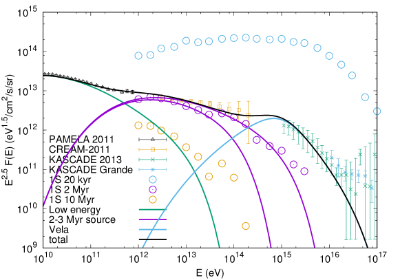
Figure 20: Contribution from the average of all Galactic (blue line and green erorbars) sources and a local source (magenta lines, for $E_{\max}=10^{14}$ and $10^{15}$ eV) to the CR proton intensity together with experimental data (orange and blue errorbars). Additionally, the flux from the local source is shown by dots for three source ages without energy cutoff.

We have already discussed that a source with age $T=2$–3 Myr and distance $R=300$  pc can explain the observed plateau in the dipole anisotropy, if its contribution to the total CR flux in this energy range is of order of one. Now we review how the model of a local source combined with anisotropic diffusion can address successfully also the spectral anomalies in the CR flux. For the age $T=2$–3 Myr, the CR density below 100 TeV is still in the quasi-Gaussian regime [215], when particle escape can be neglected. This implies an approximately energy-independent grammage crossed by CRs, explaining thereby the same slope of the secondary and proton spectra.

In Fig. 20, the proton flux of the local SN is shown with magenta lines for two values of the maximal acceleration energy, $E_{\max}=10^{14}$ and $10^{15}$ eV, respectively. The contribution to the proton flux of the background of older SNe at low energies is assumed to have the slope $\alpha=2.5$ (green line), while the contribution at higher energies (blue line) was calculated in Ref. [222]. Summing up these three contributions reproduces the observed Galactic flux of protons, represented by the data of PAMELA [182], CREAM [269], KASCADE and KASCADE-Grande [270]. Additionally to the flux at 2 Myr, the flux from the local source at 20 kyr and 10 Myr is shown. The time dependence of the observed spectrum from a single source of both the amplitude and the shape of the spectrum can be clearly seen. At early times, 20 kyr after explosion, the spectrum is close to the injected $1/E^{2.2}$ slope. The amplitude of the flux at this early time is much higher than the one observed, because it was assumed that the Earth is close to the magnetic field line going through the source. Since CRs propagate preferentially along field lines, the CR flux is enhanced compared to the isotropic case. At late times, 10 Myr, the flux is below the observed one at all energies. Note that the cutoff at high energies in the observed flux is caused by the maximal acceleration energy of the source. In contrast, the cutoff at low energies is introduced by the perpendicular distance of the Earth to the magnetic line going through the source. Since the diffusion in perpendicular direction is slow, low energy CRs did not have time to reach the Earth [223].

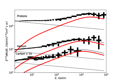
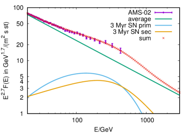
Figure 21: Left panel: The flux of CR protons, helium and carbon measured by AMS-02 and CREAM-III as function of energy/nucleon shown together with a two-component model consisting of the average CR spectrum (dotted lines) and the local source contribution (solid red lines), from Ref. [223]. Right panel: Electron flux measured by AMS-02 compared to the contributions for the local source (blue and orange lines) and average (green line) components.

In the left panel of Fig. 21, the proton, helium and carbon nuclei fluxes as function of energy per nucleon are shown together with data from the AMS-02 and CREAM experiments [223]. Each spectrum consists of two contributions: The low-energy component $F^{(1)}({\cal R})$ represents the average CR flux in the local interstellar medium, while the second component $F^{(2)}({\cal R})$ representing the CR contribution from the local SN dominates at high energies. The small differences in the abundance of nuclei in the two components—which is expected if the SN exploded in a star-forming region—is responsible for the deviations from the universality of the total flux of CR nuclei. The boron-to-carbon ratio as function of rigidity predicted in the local SN model is shown in the left panel of Fig 18. The contribution of the local SN leads to a flattening of the B/C ratio around ${\cal R}\simeq 1$ TV.

In the right panel of Fig. 21, the contribution of the local SN to the electron flux is shown. Neglecting energy losses, the contribution to the electron spectrum from the local source has the same functional form as the proton spectrum. Normalising it by choosing for the electron/proton ratio $K_{\rm ep}$ at injection $K_{\rm ep}=4\times 10^{-3}$ and adding an exponential cutoff due to energy losses gives the flux of primary electrons shown as blue line. Additionally, electrons are produced continuously by the CR protons from the local source. This contribution has a break at $\simeq 300$ GeV and is shown by the orange line. Adding finally the contribution from the background of distant sources, the observed spectrum is reproduced. The positron flux predicted in the local SN model shown in the right panel of Fig. 18 agrees also well with the data. Thus in this model, all the observational anomalies we have discussed can be understood as the imprint of a 2–3 Myr old SN on the local CR flux.

3 Cosmic rays around the knee

3.1 Observations

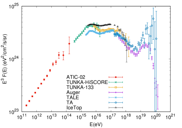
Figure 22: The all-particle CR spectrum multiplied with $E^{3}$ as function of energy together with experimental data from ATIC-2 [271], TUNKA [272], TUNKA-HiSCORE [273], IceTop [274], TALE [275], the PAO [276], and the TA [277]. All data are consistent after a 10% energy shift, i.e. within their experimental uncertainty.

The all-particle energy spectrum extending from $10^{11}$ eV up to the highest energies as measured by a few recent experiments is shown in Fig. 22. The CR intensity measured directly in satellite experiments like ATIC [271] extends smoothly into the range of indirect measurements via ground arrays and Cherenkov or fluorescence detectors like TUNKA [272], TUNKA-HiSCORE [273], IceTop  [274], TALE  [275], the PAO [276] and the TA [277]. The spectrum can be approximated by a multiply broken power-law, with a first break at 200 GeV as discussed in the previous section. At the energy $E_{\rm k}\simeq 4$ PeV, a second pronounced change dubbed the CR knee occurs where the spectral index changes from $\beta\sim 2.7$ below to $\beta\sim 3.1$ above the knee. The second knee corresponds to a change in the spectral slope of the all-particle energy spectrum at $\simeq 5\times 10^{17}$ eV where the slope softens by $\Delta\beta\simeq 0.2$. This softening was only discovered in 1992 by the Akeno experiment [278].

The elemental composition of the CR flux below $E\sim 10^{14}$ eV is relatively well determined by direct measurements using satellite and balloon experiments. At higher energies, the low CR flux prevents direct measurements. Moreover, large fluctuations in the development of extensive air showers make the determination of the mass number of individual CR primaries very difficult. Therefore experiments present their results summing up various elements into spectra of few groups of elements, or investigate only the mean mass number $A$ of the CR flux. A frequently used quantity to characterize the composition is the mean logarithmic mass, defined as $\langle\ln A\rangle=\sum_{i}f_{i}\ln A_{i}$ with $f_{i}$ as the relative fraction of nuclei with mass number $A_{i}$. Experimentally, $\langle\ln A\rangle$ can be deduced applying three main methods: Firstly, the quantity is connected to the ratio of the number $N_{i}$ of electrons and muons measured at the ground level as $\langle\ln A\rangle\simeq C+15\log(N_{e}/N_{\mu})$. The coefficient $C$ has to be determined with the help of Monte Carlo simulations for hadronic interactions and is therefore model dependent. Secondly, $\langle\ln A\rangle$ is proportional to the observed depth $X$ of the shower maximum in the atmosphere, which depends through the relation $X_{\max}^{A}=X_{\max}^{p}-D_{10}\ln A$ on the mass number $A$. Here, $X_{\max}^{p}$ and $X_{\max}^{A}$ denote the depth of the shower maximum initiated by a proton and by a nucleus with mass number $A$, respectively, while the elongation rate $D_{10}={\rm d}X_{\max}/{\rm d}\log(E)$ varies with energy between 50 and 70 g/cm². Hence, the difference in the observed depth of the shower maxima between an iron and a proton induced shower is $\simeq 100$ g/cm², what should be compared to the uncertainties from interaction models ($\Delta X\sim 25$g/cm²) and the systematic error ($\Delta X\sim 10$g/cm²) in the PAO experiment. Finally, the fluctuations of an iron induced shower are smaller than that of a proton induced shower. Thus the shape, or in first approximation, the width of the observed $X_{\max}$ distribution can be used to derive the composition. For a more detailed review of experimental methods see, e.g., the review [279, 43].

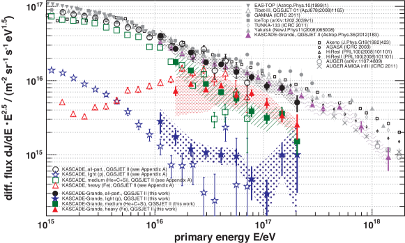
Figure 23: The CR spectrum for few elemental groups deduced from KASCADE and KASCADE-Grande date using QGSJET-II, from Ref. [280].

While there is a general agreement about the position of the knee in the total CR spectrum at $E_{\rm k}\simeq 4$ PeV, and that the composition becomes increasingly heavier in the energy range between the knee and $10^{17}$ eV [281, 282, 283, 280], there exist yet substantial uncertainties concerning the partial contributions of different mass groups to the primary CR composition. In particular, the question at which energy the suppression in the light components starts remains unclear. The results from KASCADE and KASCADE-Grande which as first experiments presented energy spectra for individual groups of elements, suggested a proton knee around 4 PeV. The spectra for the heavier elements were consistent with a rigidity-dependent knee following $E_{k}^{(Z)}=ZE_{p}$, cf. with Fig. 23. Since these results were obtained by measuring the number of electrons and muons on the ground, a rather large dependence on the used Monte Carlo simulation resulted. In particular, the relative fraction of light elements changed considerably going, e.g., from QGSJET-II-02 to Sybill. Moreover, the results of KASCADE and KASCADE-Grande are hampered by large fluctuations, since the experiment was close to sea-level.

Conflicting results for the knee in the flux of light elements were obtained by experiments using air shower arrays at high altitudes. Earlier results from CASA-MIA, BASJE-MAS, and Tibet AS$\gamma$ suggested that the suppression of the proton flux starts at 500 TeV, i.e. earlier than the knee in the total spectrum. Similar results have been obtained by the ARGO-YBJ experiment. This experiment combined results from its ground array having a large coverage with a wide field of view Cherenkov telescope. The left panel of Fig. 24 shows the knee-like structure in the combined p+He flux around 700 TeV obtained in these hybrid measurements [284], while the right panel compares the p+He flux with the all-particle spectrum. Note that for experiments at high altitudes like ARGO-YBJ on one hand the fluctuations in the electron number at ground are reduced, but on the other hand the shower maximum is close to the ground level. Moreover, fluctuations in the muon number are large, because most charged pions have no time to decay.

Finally, we want to stress the importance of determining the knee energy in the flux of the light elements. The combined p+He flux is dominated by the He component. Thus the ARGO-YBJ results would imply for the energies of a rigidity-dependent knee $E_{\rm p}\simeq 0.53$ PeV and $E_{\rm Fe}\simeq 20$ PeV. Associating these relatively low values with the maximal energy of typical Galactic CR sources reduces—at a first glance—considerably the pressure on acceleration models. However, if the source spectra would have an exponential cut-off at the rigidity ${\cal R}\simeq 0.53$ PV, then the Galactic CR spectrum would end well below 0.1 EeV. This would require either an additional Galactic component, or an extremely early transition to extragalactic CRs. In the first case, a new type of Galactic CR sources able to accelerate to such energies is needed, and the acceleration problem reappears. Requiring instead the presence of extragalactic CRs at such low energies is problematic, because they may be hidden by magnetic horizons. If on the other hand the proton knee is at $E_{\rm p}\simeq 4$ PeV, typical Galactic CR sources should be PeVatrons and an additional Galactic component at high-energies may be avoided. Moreover, knowing the energy of the knee may help to exclude some models: For instance, an energy of the proton knee as low as $E_{\rm p}\simeq 0.5$ PeV is difficult to achieve in models which explain the knee by propagation effects, as it would require too small correlation lengths of the turbulent magnetic field.

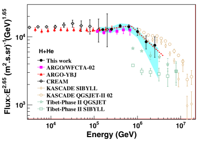
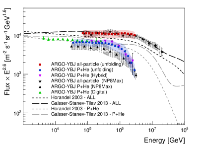
Figure 24: Left panel: H+He spectrum obtained by the hybrid experiment with ARGO-YBJ and the imaging Cherenkov telescope. The p+He spectra by CREAM [269], ARGO-YBJ [285] and the hybrid experiment [284] below the knee, the spectra by Tibet AS [286] and KASCADE [282, 280] above the knee are shown for comparison. Right panel: The all-particle and proton plus helium energy spectra measured by ARGO-YBJ by using different experimental techniques; from Ref. [287].

3.2 Models

Explanations for the origin of the knee fall in three main categories. In the first one, it was speculated that a sudden change in hadronic interactions above 2 TeV in the center-of-mass system leads to the observed change of the CR spectral slope at the knee. Alternatively, the CR flux may be suppressed above the knee because of the opening of additional energy loss channels. These possibilities were excluded by measurements at the Large Hadron Collider (LHC) which have not revealed any strong deviation from the expected characteristics of hadron production at multi-TeV energies [288]. In the second class of models, the knee is connected to properties in the energy spectrum of the Galactic CR sources. For instance, the knee might correspond to the maximal rigidity to which CRs can be accelerated by the population of Galactic CR sources dominating the CR flux below PeV [289, 290, 175]. Alternatively, the knee may be caused by a break in the source CR energy spectrum at this rigidity [291, 108]. A variant of this model is the suggestion that the spectrum below the knee is dominated by a single, nearby source and that the knee correspond to the maximal energy of this specific source. Finally, the knee could be connected to a change in the propagation of Galactic CRs. Such a change might be induced by a transition from pitch angle scattering to Hall diffusion or drift along the regular magnetic field [292, 293, 294]. Another possibility is the case suggested in Ref. [156, 222] that the knee energy corresponds to the rigidity at which the CR Larmor radius $R_{\rm L}$ is of the order of the correlation length $L_{\rm c}$ of the turbulent magnetic field in the Galactic disk. In both cases, as a result a transition from large-angle to small-angle scattering or Hall diffusion is expected, as visible in Fig. 5. Therefore the energy dependence of the confinement time changes which in turn induces a steepening of the CR spectrum [295, 292, 293, 294, 156, 222]. All these models except the first (excluded) one lead to a rigidity-dependent sequence of knees at $ZE_{\rm k}$, a behaviour first suggested by Peters [296, 297]. Measurements of the nuclear composition of the CR flux can therefore not distinguish between them. In contrast to models in category 2, those of category 3 predict both the position of the knee and the rigidity dependent suppression of the different CR components for a given model of the Galactic magnetic field [156, 222].

Maximal energy of source populations

Two specific examples for the models inside class 2 are the ones proposed by Hillas [175] and by Zatsepin et al. [144]. Such models require at least two populations of Galactic CR, one dominating the CR spectrum below and one above the knee. A natural explanation associates these two populations with two different types of SN progenitors: Cosmic rays below the knee might be accelerated, e.g., in SN explosions of isolated stars with masses $M=8-15M_{\odot}$, while CRs with higher energy are generated by massive OB or Wolf-Rayet stars in superbubbles [144]. A characteristic feature of this model is a fast change of the mass composition around $10^{16}$ eV, as it is visible in its prediction for $\ln(A)$ shown in Fig. 25.

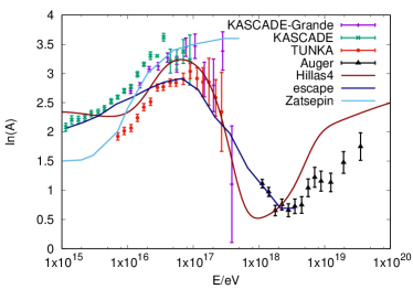
Figure 25: Predictions for $\ln(A)$ in the Zatsepin et al. [144], in the Hillas $4^{\ast}$ [298] and in the escape model [156, 222] compared to experimental data.

Another often used model is an updated variation of the Hillas model presented in Ref. [298]. The model takes into account the hardening of the CR spectrum above 200 GV and uses as cutoff for the first population 120 TV. The second population accelerates CRs up to the knee, while two additional populations of extragalactic CRs dominate the CR flux above ${\rm few}\times 10^{17}$ eV. The all-particle spectrum and the individual contributions of five groups of nuclear elements in this model are shown in the left panel of Fig. 26 for the case called $4^{\ast}$ with four populations. The third population in this model contains only proton and iron, and, in order to improve the predicted $\ln(A)$ value, a fourth population containing only protons was added. In Fig. 25, we compare the prediction for this case to experimental data of $\ln(A)$ and a good agreement is visible. However, such a two-component mixture of protons and irons is in contradiction to the narrow width RMS($X_{\max})$ of observed air showers in the atmosphere, as we will discuss in Section  4.1.2.

In the model of Ref. [299], two alternatives as explanation for a second component of Galactic CRs above the knee were investigated. In the first one, CRs are re-accelerated at the termination shock of a Galactic wind, while in the second one SN explosions of Wolf-Rayet stars lead to a CR component with an exponential cutoff of protons at $E_{\max}\simeq 1.5\times 10^{17}$ eV. The latter model leads to a large contribution of intermediate elements like helium and carbon in the CR spectrum. As we will discuss in the next section, the prediction of a large helium and CNO fraction in the energy range around $10^{17}$ and $10^{18}$ eV in the Wolf-Rayet model is in line with composition measurements of, e.g., the PAO. However, such a light or intermediate component has to be extragalactic, since otherwise the limits on the dipole amplitude will be violated [300].

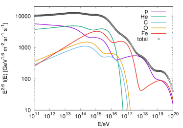
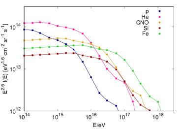
Figure 26: All-particle CR spectrum $E^{2.6}I(E)$ and individual contributions of five elemental groups as a function of the energy. Left panel for the Hillas model from Ref. [298]; right panel for the “escape model” from Ref. [156, 222].

Break in the source energy spectrum

The knee may be caused alternatively by a break in the injection spectrum $Q({\cal R})$ of Galactic CR sources [291, 108]. Typically, one models the end of the CR injection spectrum $Q({\cal R})$ by an exponential cutoff, induced either by the finite life-time or size of the accelerator. However, the shape of the cutoff depends strongly on the escape conditions, as it was shown, e.g., in Ref. [301] using Monte Carlo toy models. Since the injection efficiency and the shock velocity, and thus the maximal acceleration energy, are time-dependent, a break could be also caused by the transition from the free-expansion to the Sedov-Taylor phase of the SNR. In particular, a steepening of the injection spectrum at ${\cal R}_{\rm br}=2$ PV by $\Delta\beta=0.9$ was found in Ref. [291]: Including strong field amplification as suggested by Bell and Lucek [24, 25] into a toy acceleration model, these authors found a break in the energy spectrum of accelerated protons, coinciding for typical values SNR parameters with the knee region. The strength $\Delta\beta$ of the steepening depends among others on the injection history, and in a typical test particle ansatz $\Delta\beta=0.9$ was found. Similar results were obtained by Ref. [108]. While the steepening in the spectrum of a single source is thus too hard, a superposition of sources with varying break energies may lead to a break in the total flux compatible with observations. We conclude therefore that the often presented conclusion that a second Galactic population of CR sources above the knee is required is based on the assumption of a hard, exponential cutoff. In contrast, a single class of sources may explain the CR below and above the knee, if the high-energy tail of these sources is sufficiently strong.

A steepening of the source energy spectrum was found also in the model of massive stars exploding into their winds [302, 141]. These supernova produce two CR components: One shaped by only diffusive shock acceleration with a flat energy spectrum and a cutoff close to the knee, and second component accelerated additionally by drift acceleration and a steeper spectrun close $E^{-3.2}$. Thus the predicted spectral slope above the knee agrees well with the observed one.

Single source

In Ref. [303, 304], Erlykin and Wolfendale suggested that the CR flux in the knee region is dominated by a single young nearby source. They argued that the sharpness of the knee requires the dominance of a single source, since the unavoidable spread in the properties of, e.g., SN progenitors and environments would lead to a corresponding spread in their maximal energies, thereby smoothing out the break. In an up-dated version of this model, they suggested Vela, a SNR with the age $T\simeq 11000$ yr and distance $R=270$ pc, as a possible source candidate [305].

Vela is connected with the Solar system by a magnetic field line in models of the global Galactic magnetic field as, e.g., the Jansson–Farrar model [155]. In the case of anisotropic diffusion, CRs propagate preferentially along the magnetic field lines and thus the locally observed CR flux from Vela would be strongly enhanced: The resulting flux shown in Fig. 20 by the blue circles for $T=10^{4}$ yr overshoots the locally measured one by three orders of magnitude. Such an excess is avoided, if one takes into account that the Sun is located inside the Local Bubble: In Ref. [154], the Local Bubble was modelled as a cylinder with base radius $R=100$ pc, a bubble wall of thickness to $w=3$ pc and $B_{\rm sh}=12\mu G$, and $B_{\rm out}=1\mu G$ outside the bubble. The Sun was assumed to be at the centre of the Local Bubble, while Vela was set at the distance 270 pc from the Sun along the magnetic field. In the left panel of Fig. 27, the resulting CR flux of protons close to Vela, in the bubble wall and at Earth is shown. While at high energies, when the CR Larmor radius is large compared to the thickness of the bubble wall, the bubble wall is transparent, protons start to be trapped in the wall around $E\sim 1$ PeV. At lower energies, the flux inside the bubble is increasingly suppressed. In the right panel of Fig. 27, we show the resulting all-particle flux from Vela together with the flux from a 2–3 Myr old SN in the model of Refs. [215, 223]. The combined flux of these two sources covers the energy range from 200 GeV up to the extragalactic transition region, fitting well the experimental data.

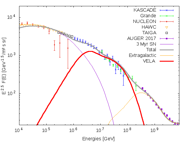
Figure 27: Left panel: The CR flux of protons around Vela, in the wall and at Earth as function of energy $E$. Right panel: The all-particle flux at Earth from a 2–3Ṁyr old SN (purple) and Vela (red) together with experimental data. Adapted from [154].

Propagation

The possibility that the knee is caused by an increased leakage of CR from the Galaxy was suggested already by Syrovatsky in 1971 [295]. Assuming for the Galactic magnetic field a strength $B\simeq{\rm few}\;\mu$G and a correlation length $L_{\rm c}\simeq 100$ pc, the transition from the diffusive to the small-angle scattering regime is expected at ${\rm few}\times 10^{16}$ eV. Thus for such parameters, the energy range of the knee can be studied in the diffusion approach. In Refs. [292, 293, 294], it was assumed that the knee corresponds to a transition between the dominance of pitch angle scattering to Hall diffusion or drift along the regular field. Since the diffusion coefficients derived for conventional pitch angle scattering and hall diffusion have different energy slopes, the cross over between the two diffusion scenarios will lead to a corresponding change in the energy spectrum of Galactic CRs. While Ref. [292] used a simplistic spatial dependence for the diffusion coefficient, [293, 294] employed a more realistic model for the GMF. The diffusion coefficients used in the latter work were extracted from the numerical results obtained in [92]. The mean $\ln(A)$ predicted in this model for the energy range $10^{15}-10^{17}$ eV agrees well with observations.

The escape model developed in Refs. [156, 222] is an alternative approach which connects the knee also with a change in the propagation of Galactic CRs. In contrast to previous works, the escape of CRs from our Galaxy was studied in these works calculating trajectories of individual CRs in models of the regular and turbulent Galactic magnetic field like the models of Pshirkov et al. or of Jansson-Farrar [70, 71]. For a correlation length $L_{\rm c}\simeq(2-5)$ pc of the turbulent field and a weak turbulent magnetic field, a knee-like structure at $E/Z={\rm few}\times 10^{15}$ eV was found, which is sufficiently strong to explain the proton knee observed by KASCADE. The resulting intensity of four other elemental groups are shown in the right panel of Fig. 26. They are consistent with the energy spectra of CR nuclei determined by KASCADE and KASCADE-Grande. Moreover, the strength of the turbulent GMF component was such that at low energies the B/C data could be successfully reproduced.

4 Transition from Galactic to extragalactic cosmic rays

4.1 Observations

We restrict our discussion to the basic experimental results, concentrating mainly on those measurements which help to understand the transition between Galactic and extragalactic CRs discussed in the next subsections. We consider the energy range above $10^{17}$ eV which corresponds roughly to the lower energy cut in most experimental analyses performed at the PAO and TA. Moreover, we will later argue that the transition between Galactic and extragalactic CRs takes place around $5\times 10^{17}$ eV. Choosing $10^{17}$ eV as the lower end of the energy range considered guaranties thus that all measurements relevant for the transition are included. To be definite, we call all particles above $10^{17}$ eV ultra-high energy cosmic rays (UHECR).

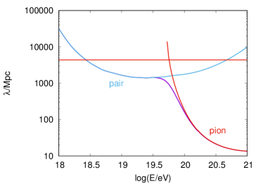
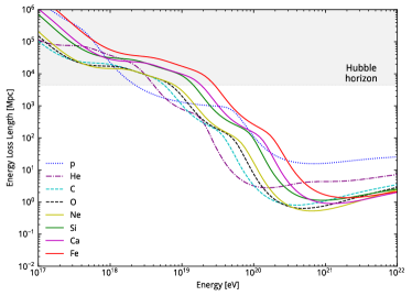
Figure 28: Left panel: The energy-loss horizon $\lambda$ of UHECR protons as function of energy. Right panel: Energy-loss horizons of different UHECR nuclei derived from CRPropa [306, 307] as function of energy.

4.1.1 Energy spectrum

Interactions of UHE protons with the cosmic microwave background (CMB) leave their imprint on the UHECR energy spectrum in the form of the Greisen-Zatsepin-Kuzmin (GZK) cutoff [308, 309], a bump and a dip [310, 311, 312, 313]. The GZK cutoff is a very pronounced steepening of the proton spectrum at the energy $E_{\rm GZK}\simeq(4-5)\times 10^{19}$ eV, caused by photo-pion production due to interactions of UHE protons with CMB photons. This effect was predicted one year after the discovery of the CMB in 1966 by Greisen and independently by Zatsepin and Kuzmin. It implies that at the highest energies only local sources within $\simeq 100$ Mpc can contribute to the observed UHECR flux.

In the left panel of Fig. 28, the energy-loss horizon

$$\lambda_{\rm hor}(E,z=0)=\left(\frac{1}{E}\frac{{\rm d}E}{c{\rm d}t}\right)^{-1}$$

for protons as function of energy is shown. The losses are caused by three processes which dominate in different energy ranges: Pion production at the highest energies, $e^{\pm}$ pair production in the intermediate energy range $3\times 10^{18}{\rm eV}\raise 1.29167pt\hbox{$\;<$\kern-7.5pt\raise-4.73611pt\hbox{$\sim\;$}}E\raise 1.29167pt\hbox{$\;<$\kern-7.5pt\raise-4.73611pt\hbox{$\sim\;$}}5\times 10^{19}$ eV, and redshift losses due to the expansion of the Universe. Note that the energy losses at the redshift $z>0$ can obtained by a simple rescaling from the present ones, $\lambda_{\rm hor}(E,z)^{-1}=(1+z)^{3}\lambda_{\rm hor}^{-1}((1+z)E,z=0)$, since they are caused by CMB photons. The GZK cutoff is caused by the strong increase of the pion production rate through the resonant process $p+\gamma_{\rm CMB}\to\Delta^{+}\to p+\pi^{0}$, when the peak of the Planck distribution of CMB photons is above threshold and participates in this reaction. While the suppression is very pronounced, the shape of this steepening is strongly model-dependent and difficult to distinguish from, e.g., a cutoff due to the maximal acceleration energy in the UHECR sources. Interacting with the CMB, protons lose energy and accumulate in the form of a bump at the energy $E_{\rm b}<E_{\rm GZK}$. These bumps are clearly seen in the spectra calculated for single sources, but disappear in the diffuse spectrum, because bumps from sources at different distance are located at different energies. The dip visible in $\lambda_{\rm hor}$ is produced by $p+\gamma_{\rm CMB}\to p+e^{+}+e^{-}$ interactions, which leads to a corresponding spectral feature in flux of UHECR protons.

In the right panel of Fig. 28, the energy loss distances of different UHECR nuclei as function of energy are shown. The main energy loss processes of nuclei are the photo-disintegration on CMB photons at high energies and on infra-red photons at lower energies. Only iron nuclei can travel distances comparable to those of protons, around 100 Mpc, at the highest energies $E\raise 1.29167pt\hbox{$\;>$\kern-7.5pt\raise-4.73611pt\hbox{$\sim\;$}}10^{20}$ eV. Thus for any composition, one expects a cutoff in the UHECR energy spectrum. While the existence of this cutoff was long time debated, it was experimentally confirmed by the HiRes experiment in 2007, 41 years after its prediction [314]. It is still unclear if the cutoff is caused by the maximal energy of sources or by the GZK effect. In the case of UHECR protons, a second dip at $6\times 10^{19}$ eV was suggested as model-independent probe for the GZK effect [315]. However, an observation of this narrow dip would require a much larger statistics than presently available, in particular if the proton flux is only subdominant.

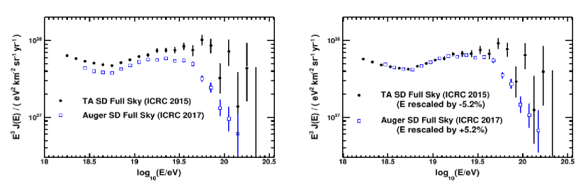
Figure 29: UHECR spectrum measured by the PAO (Auger) and TA experiments: Left panel before and right panel after the shift in the energy scale; from Ref. [316].

In Fig. 29, we show measurements of the UHECR flux from the two most recent experiments, the PAO and the TA. The uncertainty in the absolute energy scale of these experiments is around 10%, leading to large shifts in a plot of $E^{3}F(E)$. The two experiments can be cross-calibrated using that the UHECR flux up to $10^{19.2}$ eV is very isotropic: Applying a relative shift of the energy scale of the two experiments by 10.4%, their all-particle fluxes shown in the right panel of Fig. 29 agree well up to $4\times 10^{19}$ eV. At higher energies, the deviations increase, with the cutoff in the TA spectrum shifted to higher energies. Apart from unaccounted systematic effects, the different fields-of-view of the two experiments can explain these differences: Above $4\times 10^{19}$ eV, the mean free path of UHECRs drops, such that differences in the large-scale structure (LSS) are not averaged out any longer. Since the number of UHECRs contributing to the flux decreases, differences in the maximal energies of the most important sources in the northern or southern sky can become important. Alternatively, when the cutoff is caused by the GZK effect, differences in the distance to the dominating sources in two hemispheres may cause the change in the flux observed by PAO and TA. Note that the energy $E_{1/2}\simeq 5\times 10^{19}$ eV where the integral flux drops for a pure proton composition by a factor two relative to the flux expected without pion production [313] deviates significantly from the value determined from the PAO data, $E_{1/2}\simeq(2.3\pm 0.4)\times 10^{19}$ eV. Such a low value of $E_{1/2}$ may hint towards an intermediate mass composition at the highest energies.

4.1.2 Composition

The mass composition of UHECRs can be inferred from the atmospheric depth $X_{\max}$ where the number of particles in an air shower reaches its maximum. The fluorescence technique has been used both by PAO and TA to determine $X_{\max}$ , but only the former publishes its results in a form such that they can be directly compared to model predictions. In the left panel of Fig. 30, we show the $X_{\max}$ values obtained by the PAO using fluorescence detectors (FD) as filled dots. Additionally, results from the surface array (SD) are shown as open dots. Its higher duty cycle allows one to extend the energy range, while the energy calibration using FD data avoids the use of hadronic interaction models. From the evolution of $X_{\max}$ with energy, one can conclude that the composition becomes lighter between $10^{17.2}$ and $10^{18.33}$ eV, qualitatively in agreement with the expectation for a transition from Galactic to extragalactic CRs in this energy region. Above $10^{18.33}$ eV, this trend is reversed and the composition becomes heavier. The data from the Telescope Array for $X_{\max}$ shown by squares are approximately corrected for detector effects by shifting the mean by +5 g/cm² [317]. Moreover, the TA data points were shifted down by 10.4% in energy to match the energy scale of PAO [316]. After accounting for these corrections, the $X_{\max}$ data from the two experiments are in good agreement. In the right panel of Fig. 30, we show the width RMS($X_{\max})$ of the $X_{\max}$ distributions. Again, the RMS($X_{\max})$ distribution from TA has to be corrected for the detector resolution by subtracting as $X_{\max}$ resolution 15 g/cm² [318] in quadrature. A wide distribution as obtained at low energies can be caused either by a light or a mixed composition. At higher energies, the distribution becomes more narrow, pointing to a purer and heavier composition.

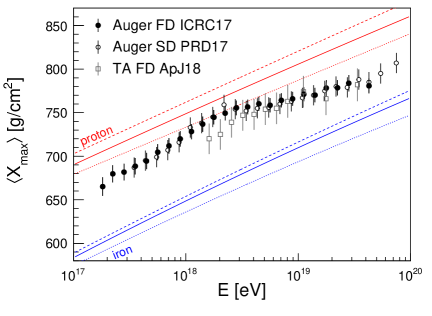
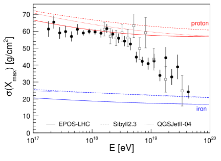
Figure 30: Measurements [319, 320, 318] of the mean (left) and standard deviation (right panel) of the distribution of shower maximum as a function of energy. The energy evolution of the mean and standard deviation of $X_{\max}$ obtained from simulations [321] of proton- and iron-initiated air showers are shown as red and blue lines, respectively; from Ref. [322].

Additionally, in both panels of Fig. 30, the predictions from three simulations for hadronic interactions are shown. All three models, QGSJET-II-04 [123, 124], EPOS-LHC [323], and SIBYLL 2.3c [324], were tuned to LHC data. The residual difference in the predictions of these models can be used as a rough estimate for the uncertainties in the theoretical predictions. Using these simulations, one can compare the predicted $X_{\max}$ distributions for a mixture of CR nuclei to the observed distribution and fit the relative fraction of the CR nuclei. The result of such a fit for a mixture of proton, helium, nitrogen and iron nuclei is shown in Fig. 31. Above $10^{18}$ eV, the dominant component in the UHECR flux changes successively from protons, to helium and nitrogen, a behaviour suggestive for the presence of a Peters’ cycle. At the lowest energies, there is evidence for a non-zero iron fraction which drops then to zero.

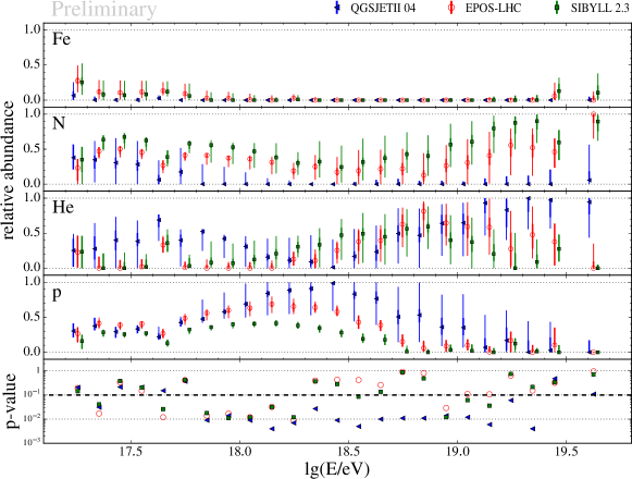
Figure 31: Fraction of the four elements in the UHECR flux; from Ref. [325].

The TA exposure is a factor 8 smaller than the one of PAO, leading to rather large statistical uncertainties in particular in analyses using the FD. Within theses errors, the data agree with the one from the PAO; for a discussion of the good overall compatibility of the $X_{\max}$ measurements from the PAO and TA see Ref. [326]. As a note of caution, we mention that Monte Carlo simulations of strong interactions as those of Refs. [123, 124, 323, 324] used to infer the mass composition cannot reproduce all details of the experimental shower measurements. In particular, data on the muon component in EAS show rather strong deviations [327], indicating that the details of a composition analysis like the one shown in Fig. 31 have to be interpreted with care.

4.1.3 Photons and neutrinos as secondaries

High-energy cosmic rays can interact with gas or photons in their sources, and with photons from the extragalactic background light (EBL) during propagation. Any process involving hadronization leads mainly to the production of pions, and isospin symmetry fixes then the ratio of charged to neutral pions produced. The production of neutrinos is thus intimately tied to the one of photons, and both depend in turn on the flux of primary CRs. Therefore the observation of these CR secondaries can provide important information on extragalactic CRs.

We discussed already in section 2.2.2 the basic properties of the secondary photon and neutrino fluxes produced in hadronic interactions on nuclei. The main difference of secondary production on background photons is the higher threshold energy $E_{\rm th}$ and the resulting suppression of the secondary flux at $E\leq E_{\rm th}$,

$${\rm d}N_{s}/{\rm d}E\sim\begin{cases}E^{-1}&\text{for $E<E_{\rm th}$},\\ {\rm d}N_{\rm CR}/{\rm d}E&\text{for $E>E_{\rm th}$}.\end{cases}$$

For instance, in p$\gamma$ interactions the threshold energy is $E_{\rm th}\raise 1.29167pt\hbox{$\;>$\kern-7.5pt\raise-4.73611pt\hbox{$\sim\;$}}m_{\pi}m_{p}/\varepsilon_{\gamma}$ with $\varepsilon_{\gamma}$ as the typical energy of the background photons. Cosmogenic neutrinos are mostly produced in interactions on EBL photons with energy $\varepsilon_{\gamma}\raise 1.29167pt\hbox{$\;<$\kern-7.5pt\raise-4.73611pt\hbox{$\sim\;$}}10$ eV. Taking into account that $\langle E_{\nu}\rangle=E_{p}/20$, this implies that the flux of cosmogenic neutrinos is suppressed below $E\approx 2\times 10^{17}$ eV. If neutrinos are produced by p$\gamma$ interactions in the source, e.g. on radiation from an accretion disk with $\varepsilon_{\gamma}\raise 1.29167pt\hbox{$\;<$\kern-7.5pt\raise-4.73611pt\hbox{$\sim\;$}}1$ eV, one expects as threshold $E_{\rm th}\approx 2\times 10^{18}$ eV. In contrast, $pp$ interactions lead to a neutrino flux without threshold.

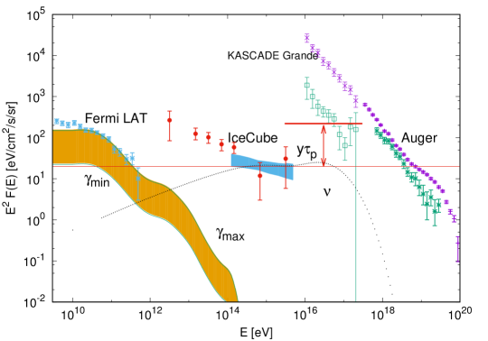
Figure 32: Expected secondary photon and neutrino fluxes from UHECR sources compared to the EGRB measured by Fermi-LAT, diffuse neutrino flux by IceCube and the all-particle and proton fluxes by KASCADE Grande and PAO. The neutrino flux example shown as thin dotted line is from Ref. [328].

Diffuse extragalactic gamma-ray background and diffuse neutrino flux

The Universe is opaque to the propagation of gamma-rays with energies in the TeV region and above. Such photons are absorbed by pair production on the EBL. As a result, the extragalactic photon flux at energies $E\raise 1.29167pt\hbox{$\;>$\kern-7.5pt\raise-4.73611pt\hbox{$\sim\;$}}1$ TeV is strongly attenuated. High-energy photons are however not really absorbed but initiate electromagnetic cascades, via the processes $\gamma+\gamma_{b}\to e^{+}+e^{-}$ and $e^{\pm}+\gamma_{b}\to e^{\pm}+\gamma$ [329, 330]. The cascade develops very fast until it reaches the pair creation threshold. Thus the Universe acts as a calorimeter for electromagnetic radiation, accumulating it in the MeV-TeV range as an extragalactic gamma-ray background (EGRB). The observed EGRB limits therefore all processes that inject electromagnetic energy.

The idea to use the EGRB to bound the neutrino flux was first suggested in Ref. [330]. In Refs.  [331, 332], measurements of the EGRB by EGRET and later Fermi-LAT were used to constrain strongly evolving UHECR models. In the meanwhile, the measurement of the EGRB was extended to higher energies [333] and, as a result, the limits on the allowed cascade radiation $\omega_{\rm casc}$ and on the cosmogenic neutrino flux dropped by a factor 3 to $\omega_{\rm casc}\leq 2\times 10^{-7}$ eV/cm³.

The main contribution to the point-source flux in Fermi-LAT is given at high energies by blazars. In Ref. [334], the contribution of unresolved sources to the ERGB was studied and it was found that the high energy part of this background is dominated by unresolved BL Lacs. The same conclusion was reached later in the more detailed study of Ref. [335]. Finally, in Ref. [336] the Fermi collaboration concluded that up to 86% of the EGRB comes from unresolved blazars. Taking these results at face value, the room for any additional injection of photons is very limited. It is therefore desirable that the same source class explains both UHECRs and the observed neutrino flux by IceCube.

In Fig. 32, we present the expectation for the secondary photon and neutrino fluxes produced by UHECR sources. The EGRB derived by the Fermi collaboration in Ref. [333] shown by blue errorbars limits the secondary photon fluxes from UHECR sources which has a universal shape indicated by the orange band [33, 337]. The total UHECR flux is shown by magenta error-bars, while the green error-bars give the flux of UHECR protons derived from the PAO and KASCADE-Grande composition measurements [325, 280]. The blue band represents the 8 years astrophysical muon neutrino flux multiplied by three and the red points the 4 years cascade neutrinos measured by IceCube [338, 339]. The horizontal thin red line shows the average neutrino flux level in the case of an $1/E^{2}$ flux, which is of the order of 10% of the EGRB. In the case of an $1/E^{2.15}$ neutrino flux, the accompanying photons saturate the gamma-ray bound, as it was first stressed in Ref. [340]. The thick red line shows the expected level of the proton flux required to produce the diffuse neutrino flux. The ratio $y\tau_{p}$ of the proton and neutrino fluxes is determined by the corresponding proton interaction probability $\tau_{p}$ and the spectrally weighted average energy tranfer $\langle y\rangle$ to neutrinos. For a spectral slope close to two, $y\sim 0.2$, implying that a large fraction of protons has to interact inside their sources.

A diffuse flux of surprisingly large magnitude was discovered by IceCube [338]: While its high-energy part is consistent with $\alpha\approx 2.1$ and a normalisation close to the cascade bound, at lower energies a softer component appears. The sources of this soft component have to be either extragalactic and hidden, or Galactic but close to isotropically distributed. Examples of extragalactic hidden sources are failed type IIn SNe [341, 342, 343], while a close to isotropic Galactic flux could be produced by decays of PeV dark matter particles, a large CR halo around the Milky Way [344, 345], or extended local neutrino sources as the wall of the Local Bubble [161]. The prime way to distinguish between these two types of solutions is the detection of the accompanying photon flux, which extends in the Galactic case up to PeV energies [346, 347]. Such a detection can be achieved, e.g., by the CARPET experiment [348].

Since the majority of neutrino sources is rather weak, an identification of neutrino sources via neutrinos multiplets has failed so far. This constraints the combination of source density and luminosity, favoring low luminosity sources [349]. However, the first source for which there is evidence of a correlation with IceCube neutrino event 170922A is the blazar TXS 0506+056, which is located at relatively high redshift $z=0.3$ [350]. There are two possible explanations: If blazars are the only dominant neutrino sources in IceCube, TXS 0506+056 at $z=0.3$ combined with the absence of high-energy neutrino multiplets [349] favors a subclass of bright BL Lacs and low luminosity FSRQ as neutrino source [351].

Alternatively, one can assume that blazars like TXS 0506+056 give a subdominant contribution, while a new class of weak sources gives the major contribution to the extragalactic IceCube signal. Because 86% of the EGRB originates from unresolved blazars, this is possible only for sources which give a minor contribution to EGRB, i.e. which have a flux $\propto 1/E^{2}$, cf. with the horizontal red line in Fig. 32. Such sources should be abundant to obey the multiplet constraint of Ref. [349], as for example star-burst galaxies or ordinary low luminosity AGNs. To avoid the additional contribution of UHECR sources to the EGRB, it is still important that such sources are major contributors to UHECR, as in the generic case of the minimal model of Ref. [328].

4.1.4 Anisotropies

The possibility to observe in the extragalactic CR flux anisotropies connected to the large-scale structure (LSS) of CR sources, or even to identify CR sources, depends on the number density $n_{s}$ of CR sources and the strength $B_{\rm exgal}$ of the extragalactic magnetic field (EGMF). If the energy-loss horizon $\lambda_{\rm hor}$ of CRs is large compared to the scale of inhomogeneities in their source distribution, then the flux of extragalactic UHECRs is isotropic in the rest frame of the CMB. In the same energy range, peculiar velocities average out on cosmological scales and the UHECR flux is thus isotropic at leading order. The movement of the Solar system with velocity $u=(368\pm 2)$ km/s with respect to the CMB results in a cosmological Compton-Getting effect with dipole amplitude

$$\delta_{\rm CG}\equiv\frac{I_{\rm max}-I_{\rm min}}{I_{\rm max}+I_{\rm min}}=\left(2-\frac{{\rm d}\ln I}{{\rm d}\ln E}\right)\,u\,.$$ (24)

Taking into account the observed spectrum $I(E)\propto E^{-2.7}$ of cosmic rays above the ankle, the numerical value of the dipole amplitude follows as $\delta_{\rm CG}=(2+2.7)\,u\simeq 0.6\%$ [352].

Moving to higher energies, the free mean path of CRs decreases and anisotropies connected to the LSS of CR sources should become more prominent and replace the cosmological Compton-Getting effect. Finally, at sufficiently high energies deflections in magnetic fields may become negligible, and a small enough number of bright point sources results in small-scale clusters of arrival directions around or near the true source positions. Depending on the actual values of $n_{s}$ and $B_{\rm exgal}$, two out of the three cases described may not be relevant: The cosmological Compton-Getting effect may be only realized at such low energies that the extragalactic CR flux is subdominant. Or sufficiently small deflections of CRs may require unrealistic high energies, where the statistics of UHECR events is too low. We start therefore this subsection with a discussion of the expected deflections of CRs in the Galactic and extragalactic magnetic fields.

Deflections of UHECRs

Propagating the distance $d$, a CR with charge $Ze$ and perpendicular momentum $p_{\perp}$ is deflected in a regular magnetic field by the angle

$$\vartheta\simeq 0.52^{\circ}Z\left(\frac{p_{\perp}}{10^{20}\,{\rm eV}}\right)^{-1}\left(\frac{d}{{\rm kpc}}\right)\left(\frac{B}{10^{-6}{\rm G}}\right)\,.$$ (25)

This formula also holds in a turbulent field for distances $d\ll L_{\rm c}$. In the opposite limit, $d\gg L_{\rm c}$, the CR propagation resembles a random walk. If the average deflection angle per correlation length $L_{\rm c}$ is small, $R_{\rm L}\gg L_{\rm c}$, the variance of the deflection angle after the distance $d$ is given by

$$\vartheta_{\rm rms}\equiv\langle\vartheta^{2}\rangle^{1/2}\simeq\frac{(2dL_{\rm c}/9)^{1/2}}{R_{\rm L}}=25^{\circ}Z\left(\frac{10^{19}{\rm eV}}{E}\right)\left(\frac{d}{100\,{\rm Mpc}}\right)^{1/2}\left(\frac{L_{\rm c}}{1\,{\rm Mpc}}\right)^{1/2}\left(\frac{B}{10^{-9}{\rm G}}\right)\,,$$ (26)

where the numerical prefactor $2/9$ was determined in Ref. [353]. The increased path-length compared to straight-line propagation leads to the time-delay

$$\Delta t\simeq\frac{d\vartheta_{\rm rms}^{2}}{4}=1.5\times 10^{3}\,{\rm yr}\,Z^{2}\left(\frac{10^{20}{\rm eV}}{E}\right)^{2}\left(\frac{d}{10\,{\rm Mpc}}\right)\left(\frac{L_{\rm c}}{1\,{\rm Mpc}}\right)\left(\frac{B}{10^{-9}{\rm G}}\right)^{2}$$ (27)

of charged CRs relative to photons [354].

Note that the increase in the path-length of CRs propagating in magnetic fields can result in the formation of a magnetic horizon [93, 355]: The maximal distance a CR can travel is in the diffusion picture given by

$$r_{\rm hor}^{2}=\int_{0}^{t_{0}}{\rm d}t\>D(E(t))=\int_{E_{0}}^{E}\frac{{\rm d}\!E^{\prime}}{\beta}\>D(E^{\prime}(t))\,,$$ (28)

where $t_{0}$ is the age of the Universe. If we consider CRs with energy below $E_{0}\raise 1.29167pt\hbox{$\;<$\kern-7.5pt\raise-4.73611pt\hbox{$\sim\;$}}10^{18}$eV, the energy losses are mainly due to the expansion of the Universe, $\beta={\rm d}\!E/{\rm d}t=-H$. For an estimate, we can use a “quasi-static” Universe, $H(t)=H_{0}$ and $t_{0}H_{0}=1$. Then $E(t)=E_{0}\exp(-H_{0}t)$ and

$$r_{\rm hor}^{2}=\frac{cL_{\rm c}}{6H_{0}}\>\left(\frac{E}{E_{\rm tr}}\right)^{2}(\exp(2)-1)\,,$$ (29)

using $D(E)=cL_{\rm c}/3\>(E/E_{\rm tr})^{2}$ valid for $R_{\rm L}\raise 1.29167pt\hbox{$\;>$\kern-7.5pt\raise-4.73611pt\hbox{$\sim\;$}}L_{\rm c}$ with $E_{\rm tr}$ defined in Eq. (16). If we assume that a magnetic field with correlation length $L_{\rm c}\sim\,$Mpc and strength $B\sim 0.1\,$nG exists in a significant fraction of the Universe, then the size of the magnetic horizon at $E=10^{18}\>$eV is $r_{\rm hor}\sim 100\,$Mpc. Hence, similar to the GZK suppression above $6\times 10^{19}\,$eV, we see a smaller and smaller fraction of the Universe for lower and lower energies. As a consequence, the spectrum of extragalactic CRs visible to us steepens at $E<10^{18}\,$eV and the extragalactic component becomes sub-dominant.

From Eqs. (25) and (26), we can estimate the deflection of CR protons with energy $E=5\times 10^{19}$ eV by the GMF. Excluding paths skimming the Galactic plane, we can set $d=500$ pc and $B=3\mu$G both for the regular and the turbulent field, resulting in a deflection $\vartheta\sim 1^{\circ}$ by the regular and $\vartheta_{\rm RMS}\sim 0.2^{\circ}$ by the turbulent Galactic magnetic field, respectively, what agrees with the results of the numerical calculations of Ref. [356]. Thus the deflection is comparable to the angular resolution of UHECR experiments, and is dominated by the deflection in the regular field. In contrast, iron nuclei would be deflected by the GMF around $30^{\circ}$ at this energy, making astronomy with heavy nuclei close to impossible. While the deflections of CR protons by the GMF should not prevent UHECR astronomy, the selection of proton events requires however an estimate of the mass number of the primary CRs on an event-by-event basis.

The impact of the EGMF on the deflections of UHECRs cannot be reliably estimated, since no convincing theory for its origin and its amplification mechanism exists. The seed fields of the EGMF could be created in the early universe, e.g. during phase transitions, and then amplified by MHD processes. Alternatively, an early population of starburst galaxies or AGN could have generated the seeds of the EGMFs at redshift between five and six, before galaxy clusters formed as gravitationally bound systems. In both cases, a large fraction of the universe may be filled with seed fields for EGMFs. Another possibility is that the ejecta of AGN magnetized the intra-cluster medium only at low redshifts, and that thus the EGMF is confined within galaxy clusters and groups. Other mechanisms have been suggested and hence no unique model with unique predictions for the EGMF exists. Simulations of the LSS including magnetic fields differ both in the input physics (seed fields, amplification mechanism), the numerical algorithms and the extraction of the results [357, 358, 359]. Therefore, it should be not too surprising that their results disagree strongly: In the simulation performed in Ref. [357], a significant fraction of all UHECRs suffers deflections comparable or larger than given by Eq. (26), while the simulation performed in [358] favour considerably smaller values. If the results of the latter simulation are closer to reality, deflections in extragalactic magnetic fields may be negligible at least for protons even at relatively low energies such as $4\times 10^{19}$ eV. Similar conclusions were obtained in Ref. [360] which studied the propagation of UHECR protons in extragalactic magnetic simulated with the cosmological ENZO code. Currently, the best upper limits in the strength of EGMFs are 1.7 nG for correlation lengths close to the Jeans scale, and 0.65 nG for correlation lengths close or larger than the observable Universe [361].

Dipole anisotropy

The (projected) dipole anisotropy $\delta$ measured by several experiments has been shown in Fig. 9 as function of energy. Below $10^{17}$ eV, the phase of the anisotropy shown in the left panel is approximately constant, except for a flip at $\simeq 200$ TeV. By contrast, at energies above $10^{17}$ eV, the phase changes smoothly towards 100 degrees in right ascension (R.A.), i.e. it points roughly towards the Galactic anticentre. This clearly suggests that the extragalactic CR flux starts at $10^{17}$ eV to become sizeable. Considering next the strength of the dipole, shown in the right panel of Fig. 9, we note that above $10^{16}$ eV only upper limits have existed until recently. Only in 2017, the PAO could detect the dipole performing a one-dimensional harmonic analysis in R.A. splitting the events in two energy bins, 4–8 EeV and $>8$ EeV [362, 174]. While the amplitude of the first harmonic in the low-energy energy bin was consistent with isotropy, the amplitude $6.5^{+1.3}_{0.9}\%$ in the second energy $>8$ EeV deviates more than 5 $\sigma$ from isotropy. Thus the observed amplitude of the dipole anisotropy is a factor 10 larger than the one predicted for the extragalactic Compton-Getting effect [352]. Higher-order harmonics like the quadrupole moment are consistent with isotropy. Therefore a combined harmonic analysis in R.A. and azimuth could be performed, and thereby the dipole vector could be reconstructed, with coordinates ${\rm R.A.}=100^{\circ}\pm 10^{\circ}$ and ${\rm dec}=-24^{\circ}\pm 13^{\circ}$. The estimated direction may be connected to an overdensity in the local galaxy distribution, seen e.g. in the 2MRS catalogue [363]. Thus the behaviour of the dipole direction suggests that the transition from Galactic to extragalactic CRs starts at $10^{17}$ eV.

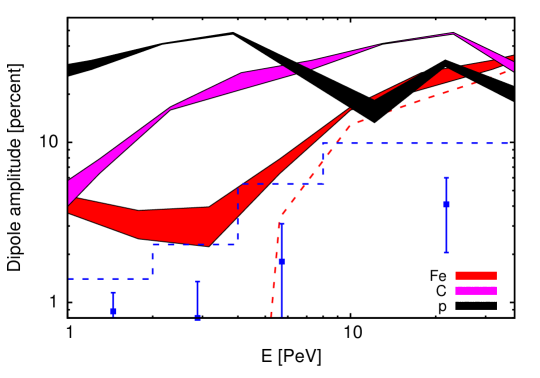
Figure 33: Predicted dipole from Galactic sources of nuclei as function of energy. The band corresponds to a variation of the vertical scale height $z_{0}$ of the turbulent GMF between 2 and 8 kpc; adapted from Ref. [300].

This conclusion can be strengthened considering the amplitude of the dipole. In Ref. [300] it was shown that a light (intermediate) Galactic CR flux leads to a dipole of order $20\%$ (10%), cf. with Fig. 33. This overshoots clearly both the limits below 8 EeV and the observed value at $>8$ EeV. Thus the dominant light-intermediate contribution to the CR flux measured by the PAO above $3\times 10^{17}$ eV has to be extragalactic. Similar results were obtained later in Ref. [364]. In both Refs. [300, 364], the trajectories of individual CRs were followed solving the Lorentz equation. In contrast, claims like the one in Ref. [365] that Galactic protons are consistent with the observed dipole amplitude are typically based on the diffusion or a simplified random walk approach which are not justified at these energies.

Medium scale anisotropies

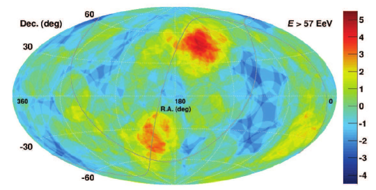
Figure 34: Sky map of UHECR events with $E>5.7\times 10^{19}$ eV from TA and PAO; the arrival directions are smeared out on circles with radius $25^{\circ}$; from Ref. [366].

Combining the data of the AGASA, HiReS, Yakutsk, SUGAR, and other experiments after rescaling their energies to a common scale, Ref. [367] found in 2005 medium scale anisotropies with 20–25 degrees scale at the $3\sigma$ confidence level. Anisotropies on such scales were seen later in the experimental data from the next generation experiments TA [368, 369] and PAO [370]. In Fig. 34, we show a sky map combining events with $E>5.7\times 10^{19}$ eV from these two experiments. The arrival directions are smeared on circles with radius $25^{\circ}$ and the colour code indicates the local significance of an over- or under-fluctuation. The most significant feature of this map is the “TA hotspot”, which is centered at ${\rm R.A.}\simeq 150^{\circ}$ and ${\rm dec}\simeq 40^{\circ}$. This direction points towards the Ursa Major supercluster; note also that the Supergalactic plane indicated by the thin line is close to the hot spot. Morover, the starburst galaxy M82 coincides with the TA hot spot. The local significance of this hot spot is $5.2\sigma$, which is reduced to $3.4\sigma$ taking into account that the spot could appear anywhere by random fluctuations [366]. An additional “warm spot” can be seen in the field-of-view of the PAO, which coincides with Cen A. Also the warm spot overlaps with the supergalactic plane.

An alternative method to search for UHECR sources are correlation studies. Several studies have shown that the distribution of the TA hotspot events is consistent with the hypothesis of a single source, the nearby starburst galaxy M82 being a promising candidate [371, 372]. The recent analysis [370] of the PAO data showed evidence for a correlation of the arrival directions of UHECRs with starburst galaxies, i.e. galaxies which are characterized by exceptionally high rates of star formation. Specifically, for UHECR with observed energies $E>39$ EeV, a model which attributes 9.7% of the UHECR flux to nearby starburst galaxies (and the remaining 90.3% to an isotropic background) was found to be favoured, with $4\sigma$ significance, over a completely isotropic test hypothesis. About 90% of the anisotropic flux was found to be associated to four nearby starburst galaxies: NGC 4945, NGC 253, M82, and NGC 1068. Alternatively, a correlation analysis with 17 bright nearby AGNs was performed. Here, the warm spot is related to Cen A and around 7% of the total flux is attributed to the selected AGNs. These claims were reassessed in a new analysis of the TA data [373], which gave results consistent with both the PAO anisotropy and with isotropy, due to the small number of events.

4.2 Transition energy

The question at which energy the transition from Galactic to extragalactic CRs takes place is fundamental to our understanding of Galactic CR sources and the requirements on their acceleration mechanisms as well as to the determination of the nuclear composition and the injection spectrum of extragalactic sources. In the past, the two most promising choices for the transition energy were to associate it with one of the evident features of the CR spectrum: The second knee around $E\simeq(1-5)\times 10^{17}$ eV or the ankle at $E\simeq 3\times 10^{18}$ eV. The latter option offered a simple explanation for the sharpness of the ankle as the cross-over between the end of Galactic flux and the start of the extragalactic component. Moreover, it allowed for an extragalactic injection spectrum $Q(E)\propto 1/E^{\beta}$ with $\beta\approx 2$, i.e. close to the theoretical expectation for diffusive shock acceleration. The main disadvantage of this suggestion is the enormous pressure it puts on acceleration models for Galactic CR sources. Moreover, this solution may lead to the following “fine-tuning problem”: Since the acceleration and diffusion of CRs is rigidity-independent, one expects that the end of the Galactic CR spectrum shows a sequence of cutoffs at $ZE_{\max}$, i.e. follows a Peter’s cycle. If the ankle is identified with the transition, it is natural to assume that the second knee corresponds to the iron knee. Thus, in this interpretation, the second knee signals the end of the Galactic iron flux from those sources which contribute the bulk of Galactic CRs. Therefore an additional Galactic population of CR sources would be required to fill the gap between the second knee and the ankle. If this population is unrelated to the standard population of Galactic CR sources, it is surprising that the normalisation of the two fluxes is so close.

The challenge of models identifying the second knee as the transition to extragalactic CRs is to find a physical mechanism which explains the ankle as a consequence of either the propagation of extragalactic CRs or of interactions in their sources. The first successful model of this kind explained the ankle by the dip in the pair-production losses of protons on cosmic microwave background (CMB) photons $p+\gamma_{\rm CMB}\rightarrow p+e^{+}+e^{-}$ [374]. This elegant possibility is however excluded by composition measurements. Only recently, the authors of Ref. [375] suggested as a viable alternative a model which relies on photo-disintegration of CR nuclei on background photons inside CR sources. Note also that from a theoretical prespective, a successful model for the transition has to address both the extragalactic and the Galactic contributions to the measured fluxes of individual groups of elements, $F_{i}^{\rm obs}(E)=F_{i}^{\rm exgal}(E)+F_{i}^{\rm gal}(E)$, since only the sum of both is observed.

How can these two options for the transition energy, the second knee and the ankle, be experimentally distinguished? It is natural to expect that the nuclear composition of Galactic and extragalactic CRs should differ, because of propagation effects and of the different nature of their sources. In particular, the Galactic CR spectrum should become close to its end iron-dominated. A similar behaviour is expected for the extragalactic flux, shifted however to higher energies. Thus one expects the extragalactic composition at the transition energy to be lighter than the Galactic one. Therefore the signature of the transition in the composition is the disappearance of the (Galactic) iron, and the increase of a light or intermediate extragalactic component. An additional powerful constraint comes from anisotropy measurements which limit a light or intermediate Galactic component.

From the data presented in the previous section, the following conclusions can be drawn: Using only the composition data, the limits on the iron fraction from Fig. 31 imply that the Galactic contribution to the observed CR spectrum has to die out before $7\times 10^{17}$ eV. The confidence in this conclusion is strengthened considerably, if one combines the composition and anisotropy measurements: In Ref. [300], it was shown that a light (intermediate) Galactic CR flux leads to a dipole of order $20\%$ (10%), overshooting clearly the limits which are on the percent level [174]. Thus the dominant light-intermediate contribution to the CR flux measured by the PAO above $3\times 10^{17}$ eV has to be extragalactic. Finally, we recall that the smooth change of the dipole phase at energies above $10^{17}$ eV towards the Galactic anticentre supports the suggestion that the transition from Galactic to extragalactic CRs starts at $10^{17}$ eV. Thus we conclude that the second knee marks the transition between Galactic and extragalactic CRs. Then it is natural that the second knee is close to its upper end of the range $(1-5)\times 10^{17}$ eV of values considered in the literature and, for definiteness, we choose $E\simeq 5\times 10^{17}$ eV for the position of the second knee.

4.3 Models for extragalactic CRs and the transition

The first concrete model able to explain the ankle as a feature of the extragalactic CR spectrum was the dip model [313, 374]. The main assumption of this model is that the extragalactic CR flux consists of protons, with a maximal admixture of $\raise 1.29167pt\hbox{$\;<$\kern-7.5pt\raise-4.73611pt\hbox{$\sim\;$}}10\%$ of helium. Then the ankle can be explained as a feature in the extragalactic CR spectrum imprinted by pair-production losses of protons on CMB photons, cf. with the energy loss rate of protons shown in Fig. 28. This elegant possibility has been however excluded by composition measurements, in particular of the PAO. It is interesting to note that meanwhile even the non-observation of cosmogenic neutrinos challenges this model [377].

Since composition measurements, in particular of the fluctuations of the shower maximum RMS($X_{\max})$, pointed to an increase of the mean mass number of CRs with increasing energy, models including nuclei were proposed as alternative. For instance, the models of Refs. [378, 379, 380] used a mixed composition together with a power-law in rigidity and an exponential cut-off, $Q({\cal R})=Q_{i}{\cal R}^{-\beta}\exp(-{\cal R}/{\cal R}_{\max})$, for the injection spectrum. These models could reproduce $X_{\max}$  and RMS($X_{\max})$ data, but lead to the ankle as transition energy. Therefore such models require an additional light extragalactic component below the ankle. The spectral index of the injection spectrum of this additional population should be steeper ($Q({\cal R})\propto{\cal R}^{-2.7}$) than the one of the population responsible for the spectrum above the ankle [381]. Again, it is surprising that the normalisation of these two contributions is so close, if these two populations are unrelated.

The end of the proton component measured by KASCADE-Grande can be extended smoothly to the one observed by the PAO by a power law with slope $\alpha\sim 2.2$, cf. with Fig. 32. Any model aiming to extend the extragalactic flux below the ankle has to explain this proton component. In Ref. [382], it was assumed that this flux reflects the original injection spectrum of protons, since the slope is consistent with the one expected from diffusive shock acceleration. It was shown that star-forming galaxies cannot explain this proton component, while BL Lacs/FR I galaxies could both provide the proton component and a dominant contribution to the observed neutrino flux and the EGRB. However, this work did not address the fluxes of heavier nuclei required by the composition measurements.

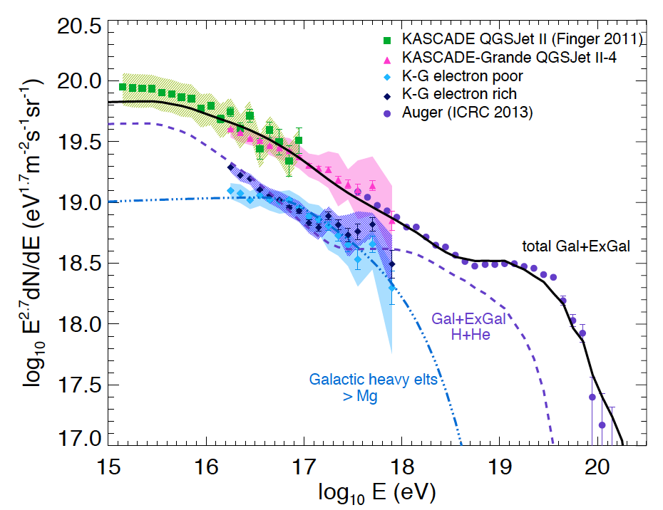
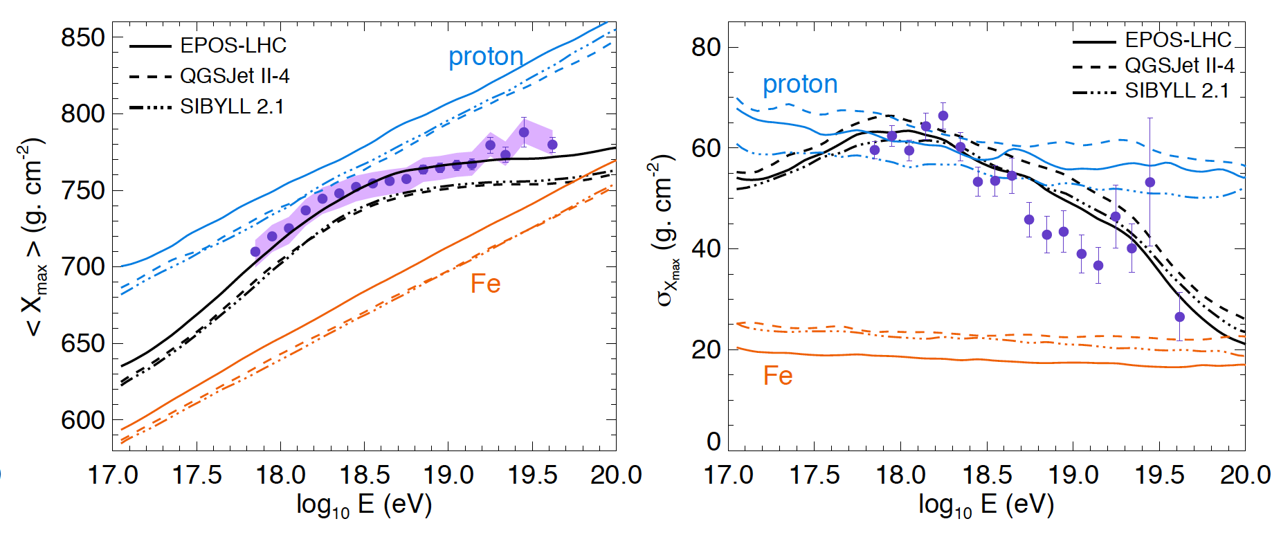
Figure 35: Left panel: Galactic and extraglactic contributions to the total CR flux in the GRB model of Ref. [383] compared to experimental data from PAO and KASCADE-Grande. Right panel: $X_{\max}$ and RMS($X_{\max})$ as function of energy in model of Ref. [383] compared to data from the PAO.

In an alternative scenario, the extragalactic proton component originates from the photo-disintegration of heavier nuclei in photon fields present in the source [384, 375]. This mechanism has been employed in a specific model of UHECR acceleration by gamma-ray bursts (GRB) in Refs. [384, 383]. In this model, the photo-disintegration of low-energy nuclei leads to a flattening of their spectra from $\beta\simeq 2.1-2.2$ to $\beta\simeq 1$. Only the proton spectrum follows the original acceleration spectrum because of a decaying neutron component which escapes from the source, cf. with Fig. 35. While the original model resulted in a transition at the ankle [384], choosing a stronger redshift evolution $Q(z)\propto(1+z)^{m}$ with $m=3.5$ for GRBs increases the extragalactic contribution below the ankle [383]. Nevertheless, the required Galactic iron fraction is , e.g., 20% at $10^{18}$ eV and thus relatively high compared to the determination from Ref. [325].

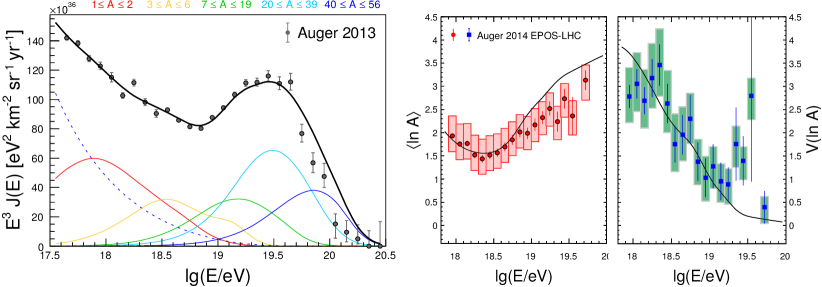
Figure 36: The energy spectrum, $\ln(A)$ and $\sigma(\ln(A))$ as functions of energy for an injection composition following a Galactic mixture. The dotted line shows the assumed Galactic flux; adapted from Ref. [375].

A generic calculation of the effect of photo-nuclear interactions in astrophysical sources was performed in Ref. [375]. In their fiducial model a hard energy spectrum, $\beta=1$, was assumed and the maximum proton energy and photon background energy were derived by fitting the UHECR data. Within a variety of source evolutions and different assumptions about the shape of the photon spectrum, the maximum energy of protons and photon background were found to be typically $E_{\max}^{p}=3\times 10^{18}$ eV and $\varepsilon_{\gamma}=0.1$ eV, respectively. A good fit to both the energy spectrum and the composition data was obtained injecting a single nuclear species with intermediate mass number like, e.g., silicon. For a more natural mixed composition of the injected CRs, the transition energy moves somewhat to higher energies, cf. with the left panel of Fig. 36. The agreement of the fit for $\ln(A)$ and the variance $\sigma(\ln(A))$ shown in the other two panels is, taking into account the large uncertainties of hadronic interactions in air showers, very good.

Both the GRB and AGN models of Refs. [383, 375] relied on interactions of nuclei with a photon background. As a result of the threshold effect described in section 4.1.3, the resulting neutrino fluxes are therefore suppressed in the interesting TeV–PeV range and cannot explain the observations of IceCube. In contrast, models leading to large neutrino fluxes in the 0.1–1 PeV energy range use typically $pp$ interactions and primaries with 10–100 PeV energies. Thus such models have no direct connection to the sources of UHECRs.

A possible way of how a single source class can explain the extragalactic CR flux, its nuclear composition and the observed neutrino flux in IceCube at the same time was suggested in Ref. [328]. The model presented there assumes that UHECRs are accelerated in the core of (a subclass of) AGNs. Subsequently, the CR nuclei diffuse first through a zone dominated by photo-hadronic interactions, before they escape into a second zone dominated by hadronic interactions with gas. In the first zone, the energy-dependence of the photo-disintegration rates and the escape times leads together with a rigidity-dependent cut-off to a rather small energy window in which a single nuclear species is unsuppressed. The flat proton component is generated again by escaping neutrons. In the second zone, on larger scales, the escaping nuclei interact on gas and produce thereby a neutrino flux which can give a substantial contribution to the flux observed by IceCube. In an alternative scenario, the photon background was assumed to have negligible impact and only $Ap$ interactions were included.

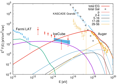
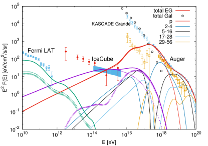
Figure 37: Diffuse flux of five elemental groups in the model of Ref. [328].

The diffuse fluxes of five elemental groups computed in this model are shown on the left panel of Fig. 37 for only $Ap$ interactions and on the right for $A\gamma$ and $Ap$ interactions. In the case of only hadronic interactions, $\beta=1.8$, $E_{\max}=3\times 10^{18}$ eV and BL Lac evolution is used, otherwise $\beta=1.5$, $E_{\max}=6\times 10^{18}$ eV, $\tau^{p\gamma}=0.29$ and AGN evolution. The hadronic interaction depth is normalised as $\tau^{pp}_{0}=0.035$ at $E=10^{19}$ eV. The diffuse fluxes are compared to experimental results for the proton (orange error-bars) and the total flux from KASCADE, KASCADE-Grande (light-blue error-bars) [280] and Auger (dark-blue error-bars) [385, 386], the EGRB from Fermi-LAT (light-blue error-bars) [333], and the high-energy neutrino flux from IceCube (light-blue shaded area) [338]. In both cases, the total CR flux including the ankle feature is well-fitted. Adding the Galactic CR flux determined in the escape model [156, 222] leads to a good description of the total flux in the transition region and below. Both cases lead to large neutrino fluxes, respecting at the same time however the EGRB limit. For illustration, the contribution of neutrinos and photons from $A\gamma$ and $Ap$ interaction is shown on the right top separately by crosses and dotted lines, respectively.

In Fig. 38, we compare the predictions of these two scenarios for $X_{\max}$ and RMS($X_{\max})$ using the EPOS-LHC [323] and QGSJET-II-04 [123, 124] models to data from Auger [387]. In the “hadronic only” scenario, insisting to reproduce the ankle requires a relatively low cut-off energy, and a small contribution of intermediate nuclei. This drives the composition towards a two-component model, consisting mainly of protons and iron. As a result, the $X_{\max}$ data above $5\times 10^{18}$ eV are not well described. Since the spectra of intermediate CNO nuclei are cut off around the ankle, their contribution could be only increased if the proton flux is reduced. But a reduction of the proton flux would in turn reduce the neutrino flux and the model will fall short of explaining the IceCube data. In contrast, the scenario including photo-disintegration reproduces the $X_{\max}$ and RMS($X_{\max})$ data well, taking into account the systematic uncertainties.

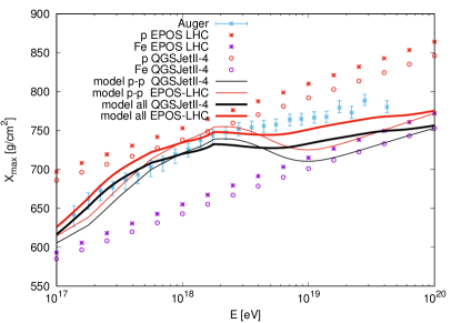
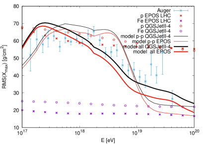
Figure 38: The resulting $X_{\max}$  (middle) and RMS($X_{\max})$ (bottom) values in the model of Ref. [328].

Finally, let us comment briefly on some other recent extragalactic CR models which attempt at the same time to account for the diffuse neutrino flux observed by IceCube. The authors of Ref. [388] explain the IceCube neutrinos by CR interactions in the galaxy clusters surrounding UHECR sources. This scheme may be considered as a concrete physical model of the “only hadronic” scenario presented above. The CR flux in this model has however no ankle feature and requires therefore a second extragalactic component. The same limitation applies to the model of Ref. [389] which suggests low-luminosity GRB as common source of UHECRs and neutrinos. The authors of Ref. [390] studied the central regions of active galaxies as sources of UHECRs. They followed the approach of Ref. [375] and concluded that low luminosity AGNs with no source evolution are favoured as UHECR sources compared to models with strong source evolution or large photon backgrounds in the source.

5 Summary and outlook

The all-particle spectrum of CRs has been measured with good accuracy up to the highest energies. Moreover, considerable progress has been made in the last decade on the more challenging task of determining the nuclear composition of the CR flux. At the highest energies, the composition results from the PAO have led to a paradigm shift, making “pure proton” models for the extragalactic CR flux nonviable. Similarly, the results in the energy range up to the knee obtained by direct detection experiments have challenged previously accepted models for Galactic CRs. In particular, the increased precision of experiments like PAMELA, CREAM and AMS-02 for the fluxes of individual nuclei as well as of electrons, positrons and antiprotons have revealed several deviations from previous expectations: The anomalies discovered include non-universal rigidity spectra of CR nuclei with a break at 300 GV, the hardening of the electron spectrum around 50 GeV and the positron excess.

A multitude of models for Galactic CRs has been developed which can explain one or several of these features. In order to distinguish between them, additional experimental data are necessary. For instance, the confirmation of a power law-like positron spectrum with a steepening by $\Delta\alpha=1$ at 300 GeV would support the idea of a 2–3 Myr old local source where the positrons are produced during propagation [215]. The related suggestion that the positrons are produced close to a younger source would lead instead to a steeper break in the positron spectrum at higher energy, $E\sim 1$ TeV [253, 255]. In contrast to this high-energy suppression, the reacceleration model of Ref. [247] predicts a rise of the positron flux with energy. If the positrons are connected instead to nearby pulsars, several bumps related to the steep high-energy cutoff of the nearest pulsars may become visible in the positron spectrum. Another prediction of most pulsar models are similar fluxes of positrons and electrons at high energies, $R_{e^{+}/(e^{-}+e^{+})}\simeq 0.5$. In contrast, antiproton and positron fluxes are unrelated in this model, and the ratio $R_{e^{+}/\bar{p}}\simeq 2$ is a mere accident. Decreasing the uncertainties in the predictions for antiproton production and testing thereby the ratio $R_{\bar{p}/e^{+}}$ more precisely is therefore an additional possibility to differentiate between hadronic and pulsar models for the positron excess.

Another important handle to distinguish models are the secondary-to-primary ratios of nuclei like B/C at high energies: While in the majority of models these ratios should continue to decrease like $E^{-1/3}$ moving to higher energies, some models predict a slower decrease as $\propto E^{-0.15}$ [256], a plateau [223] or even an increase [249]. Extending the energy range of the B/C measurements and adding additional ratios like Ti/Fe is therefore very valuable.

Higher precision in the determination of the primary (and secondary) spectra may reveal how granular the CR sea is. Since the number of CR sources contributing to the locally measured CR flux depends strongly on how anisotropic CR diffuse, this “granularity” provides an important constraint on the CR propagation. If the number of contributing sources is reduced by a factor 100 as argued in Ref. [150], only few sources may be responsible for the locally observed CR flux above 200 GeV. In this scenario, one expects also at lower energies a reduced number of sources contributing which should manifest itself by additional small breaks in the primary spectra. Similarly, the smooth B/C ratio as function of rigidity should dissolve into a series of small plateaus in this scenario, if the experimental precision is increased.

At present, the electron spectra determined by different experiments show systematic discrepancies. A more precise, consistent determination of the electron flux above 200 GeV is required to constrain the properties of local sources. The question at which energy the spectrum contains cooling breaks, and if they agree or not with those in the positron spectrum, is an important piece of information. Combining the electron and positron measurements, a ratio $R_{e^{+}/(e^{-}+e^{+})}$ much smaller than 0.5 would disfavour pulsar models.

The behaviour of the dipole anisotropy of CR nuclei as function of energy, i.e. the phase flip by $180^{\circ}$ and the plateau in the amplitude, suggests that the dipole is aligned with the local ordered magnetic field and that CRs propagate anisotropically. A measurement of the dipole phase of positrons provides therefore a test of both source and propagation models: In naive diffusion models, it is assumed that the dipole is aligned with the CR flux $\boldsymbol{j}\propto\boldsymbol{\nabla}n$. Thus the dipole should point to the (flux weighted) location of the positron sources, which are known in the case of pulsars like Geminga and PSR B0656+14. In contrast, the dipole of positrons should agree with the one of CR nuclei, if the positrons have an hadronic origin and are produced, e.g., in SNRs. Going beyond the naive diffusion approach, CRs with $R_{\rm L}\ll L_{\rm c}$ propagate anisotropically even in the absence of a regular magnetic field, since the field modes with $k/(2\pi)\gg R_{\rm L}$ act locally as an ordered field [94]. Thus one should always expect that the dipole is aligned with the local ordered magnetic field. Finally, the relative size of the dipole amplitude of positrons and nuclei can help to distinguish models.

The question how strong our nearby environment in the Galaxy, in particular the Local Bubble, influences local measurements has not attracted much attention yet. The effect of the Local Bubble might be particularly important for recent nearby sources as Vela and for the interpretation of the CR dipole: The increased magnetic field in the bubble wall may surppress at low-energies the flux from young, nearby sources and reduce anisotropies by spreading CRs on the wall. Additionally, the interactions of CRs in the dense walls of the Local Bubble and Loop I have been suggested as sources of an extended Galactic neutrino emission.

Another important requisite in advancing propagation models are improved models of the global GMF and an enhanced understanding of magnetic turbulence. The advance of the SKA radio telescope array will dramatically increase the number of RMs of extragalactic sources from 42.000 to tens of millions, while pulsar RMs are expected to increase from 1133 to 18.000 [391]. This enormous increase of input data should in combination with more sophisticated analysis methods [69] allow one to improve considerably the reliability of models for the global GMF. On the theoretical side, an important open issue is the nature and importance of magnetic turbulence. While it seems natural that at sufficiently low energies self-generated turbulence becomes more important than the turbulence injected by SNe and stellar winds, the transition energy between these two regimes is unknown. Moreover, the theoretical understanding of magnetic turbulence is rather incomplete [57], and a self-consistent description of the coupling at low energies between the CR fluid, magnetic fields and the ISM is largely unexplored.

An important objective of new experiments like LHAASO [392] or the the extension of IceTop [393] is the measurement of the mass composition in the knee region and above. In particular, the resolution of the position of the proton knee—which is at present discrepant between different experiments—is from a theoretical point crucial in pinning down the maximal energy and the possible need for an additional population of Galactic CR sources. Moreover, a better knowledge of the mass composition close to the second knee is needed to constrain models for the extragalactic CR flux.

There has been considerable experimental progress at higher energies. In particular, a cut-off in the energy spectrum of UHECRs has been firmly established although its nature is yet unclear: Both the finite maximal acceleration energy in the sources and GZK-like interactions of nuclei on background photons may be the cause. The energy spectrum derived by PAO and TA agree well within their systematic uncertainties, except for the highest energies where the differences may be caused by the different field-of-view. The determination of the mass composition of UHECRs has progressed by the much larger statistics of fluorescence events available which allowed TA and PAO to go beyond the analysis of the average $X_{\max}$ . In particular, using the full information contained in the $X_{\max}$ distribution allowed the PAO collaboration to fit the fraction of four elements in the CR flux. While these results have to be taken with some caution, they suggest the presence of a Peters’ cycle above $2\times 10^{18}$ eV. In the near future, the low-energy extensions and upgrades of the TA [394] and the PAO [395] will allow one to test this scenario with increased accuracy.

While in the energy range $10^{16}-8\times 10^{18}$ eV only upper limits on the dipole anisotropy exist, the dipole vector with an amplitude $6\%$ has been measured by the PAO using events with energy $\geq 8\times 10^{18}$ eV. Its direction points away from the Galactic centre and is roughly consistent, taking into account deflections in the GMF and EGMF, with an overdensity in the local galaxy distribution. On smaller scales, the most prominent deviation from isotropy is the TA hot spot. Additionally, the PAO claims evidence for correlations of the UHECR arrival directions with specific types of CR sources, as e.g. starburst galaxies. At present it is however unclear if these correlations do not simply reflect the nearby large-scale structure.

Three pieces of evidence can be used to determine the energy at which the transition from Galactic to extragalactic CRs takes place. First, the behaviour of the dipole anisotropy suggests that the transition starts at $10^{17}$ eV. Second, the disappearance of the iron component at $5\times 10^{17}$ eV in the PAO composition data signals the end of the Galactic CR spectrum. Finally, combining the composition and anisotropy measurements, one can conclude that the dominant light-intermediate contribution to the CR flux measured above $7\times 10^{17}$ eV has to be extragalactic. Taking into account these different pieces of evidence, we have concluded that the transition from Galactic to extragalactic CRs happens at the second knee, i.e. around $5\times 10^{17}$ eV.

Using Occam’s razor, one may dismiss the possibility that the ankle is the cross-over of the fluxes of two independent extragalactic populations of UHECR sources. Then the ankle has to be explained as a consequence of either the propagation of extragalactic CRs or of interactions in their sources. The dip model which relied on the first possibility is excluded by composition measurements. A viable alternative uses photo-disintegration of CR nuclei on background photons inside their sources, which might be either AGN cores or GRBs. Successful models tend to have built-in unusual features as steep injection spectra or a large contribution of injected nuclei with intermediate mass number which wait for a physical motivation. Requiring additionally that these UHECR sources explain the neutrino flux measured by IceCube poses another challenge. Developing concrete models which reproduce all the experimental data which have become available in the last years will be an important step towards understanding the sources of UHECRs.

References

- [1] C. A. de Coulomb, Troisième Mémoire sur l’Electricité et le Magnétiseme, Histoire de l’Académie Royale des Sciences (1785) 612–638.
- [2] V. F. Hess, Über Beobachtungen der durchdringenden Strahlung bei sieben Freiballonfahrten, Phys. Z. 13 (1912) 1084–1091.
- [3] J. Clay, Penetrating Radiation, Proc. Kon. Akademie (Amsterdam) 30 (9-10) (1927) 1115–1127.
- [4] W. Bothe, W. Kolhörster, Das Wesen der Höhenstrahlung, Z. Phys. 56 (1929) 751–777. doi:10.1007/BF01340137.
- [5] M. Schein, W. P. Jesse, E. O. Wollan, The Nature of the Primary Cosmic Radiation and the Origin of the Mesotron, Phys. Rev. 59 (1941) 615. doi:10.1103/PhysRev.59.615.
- [6] W. Kolhörster, I. Matthes, E. Weber, Gekoppelte Höhenstrahlen, Naturwissenschaften 26 (1938) 576–576. doi:10.1007/BF01773491.
- [7] P. Auger, P. Maze, T. Grivet-Meyer, Grandes gerbes cosmiques atmosphériques contenant des corpuscules ultra-pénétrants, Comptes Rendus de l’Académie des Sciences 206 (1938) 1721.
- [8] G. V. Kulikov, G. B. Khristiansen, On the Size Spectrum of Extensive Air Showers, J. Exp. Theor. Phys. 35 (1958) 8.
- [9] J. Linsley, Evidence for a primary cosmic-ray particle with energy eV, Phys. Rev. Lett. 10 (1963) 146–148. doi:10.1103/PhysRevLett.10.146.
- [10] W. Baade, F. Zwicky, Cosmic Rays from Super-novae, Proceedings of the National Academy of Science 20 (1934) 259–263. doi:10.1073/pnas.20.5.259.
- [11] W. A. Hiltner, Polarization of Radiation from Distant Stars by the Interstellar Medium, Nature 163 (1949) 283. doi:10.1038/163283a0.
- [12] J. S. Hall, Observations of the Polarized Light from Stars, Science 109 (1949) 166–167. doi:10.1126/science.109.2825.166.
- [13] E. Fermi, On the Origin of the Cosmic Radiation, Phys. Rev. 75 (1949) 1169–1174. doi:10.1103/PhysRev.75.1169.
- [14] P. Morrison, S. Olbert, B. Rossi, The Origin of Cosmic Rays, Phys. Rev. 94 (2) (1953) 440–453. doi:10.1103/PhysRev.94.440.
- [15] V. L. Ginzburg, S. I. Syrovatskii, The origin of cosmic rays, New York: Gordon and Breach, 1969.
- [16] W. I. Axford, E. Leer, G. Skadron, The acceleration of cosmic rays by shock waves, International Cosmic Ray Conference 11 (1977) 132–137.
- [17] R. D. Blandford, J. P. Ostriker, Particle Acceleration by Astrophysical Shocks, Astrophys. J. 221 (1978) L29–L32. doi:10.1086/182658.
- [18] G. F. Krymskii, A regular mechanism for the acceleration of charged particles on the front of a shock wave, Akademiia Nauk SSSR Doklady 234 (1977) 1306–1308.
- [19] A. R. Bell, The acceleration of cosmic rays in shock fronts. I, Mon. Not. Roy. Astron. Soc. 182 (1978) 147–156.
- [20] L. O. Drury, An introduction to the theory of diffusive shock acceleration of energetic particles in tenuous plasmas, Rept. Prog. Phys. 46 (1983) 973–1027. doi:10.1088/0034-4885/46/8/002.
- [21] A. M. Hillas, The Origin of Ultra-High-Energy Cosmic Rays, Ann. Rev. Astron. Astrophys. 22 (1984) 425–444. doi:10.1146/annurev.aa.22.090184.002233.
- [22] J. R. Jokipii, Rate of energy gain and maximum energy in diffusive shock acceleration, Astrophys. J. 313 (1987) 842–846. doi:10.1086/165022.
- [23] P. O. Lagage, C. J. Cesarsky, The maximum energy of cosmic rays accelerated by supernova shocks, Astron. Astrophys. 125 (1983) 249–257.
- [24] A. R. Bell, S. G. Lucek, Cosmic ray acceleration to very high energy through the non-linear amplification by cosmic rays of the seed magnetic field, Mon. Not. Roy. Astron. Soc. 321 (2001) 433–438. doi:10.1046/j.1365-8711.2001.04063.x.
- [25] A. R. Bell, Turbulent amplification of magnetic field and diffusive shock acceleration of cosmic rays, Mon. Not. Roy. Astron. Soc. 353 (2004) 550–558. doi:10.1111/j.1365-2966.2004.08097.x.
- [26] E. G. Berezhko, L. T. Ksenofontov, H. J. Völk, Confirmation of strong magnetic field amplification and nuclear cosmic ray acceleration in SN 1006, Astron. Astrophys. 412 (2003) L11–L14. arXiv:astro-ph/0310862, doi:10.1051/0004-6361:20031667.
- [27] J. Vink, J. M. Laming, On the magnetic fields and particle acceleration in Cas A, Astrophys. J. 584 (2003) 758–769. arXiv:astro-ph/0210669, doi:10.1086/345832.
- [28] A. Bamba, R. Yamazaki, T. Yoshida, T. Terasawa, K. Koyama, A Spatial and spectral study of nonthermal filaments in historical supernova remnants: Observational results with Chandra, Astrophys. J. 621 (2005) 793–802. arXiv:astro-ph/0411326, doi:10.1086/427620.
- [29] M. Kachelrieß, Lecture notes on high energy cosmic raysarXiv:0801.4376.
- [30] K. V. Ptitsyna, S. V. Troitsky, Physical conditions in potential sources of ultra-high-energy cosmic rays. I. Updated Hillas plot and radiation-loss constraints, Phys. Usp. 53 (2010) 691–701. arXiv:0808.0367, doi:10.3367/UFNe.0180.201007c.0723.
- [31] M. Spurio, Probes of Multimessenger Astrophysics, Astron. Astrophys. Lib. 9783319968544 (2018) pp.1–591. doi:10.1007/978-3-319-96854-4.
- [32] B. P. Abbott, et al., Multi-messenger Observations of a Binary Neutron Star Merger, Astrophys. J. 848 (2) (2017) L12. arXiv:1710.05833, doi:10.3847/2041-8213/aa91c9.
- [33] V. S. Berezinsky, S. V. Bulanov, V. A. Dogiel, V. S. Ptuskin, Astrophysics of cosmic rays, Amsterdam, Netherlands: North-Holland, 1990.
- [34] R. Schlickeiser, Cosmic ray astrophysics, Berlin: Springer, 2002.
- [35] T. K. Gaisser, R. Engel, E. Resconi, Cosmic Rays and Particle Physics, Cambridge University Press, 2016.
- [36] M. Potgieter, Solar Modulation of Cosmic Rays, Living Rev. Solar Phys. 10 (2013) 3. arXiv:1306.4421, doi:10.12942/lrsp-2013-3.
- [37] A. Marcowith, et al., The microphysics of collisionless shock waves, Rept. Prog. Phys. 79 (2016) 046901. arXiv:1604.00318, doi:10.1088/0034-4885/79/4/046901.
- [38] A. M. Bykov, D. C. Ellison, A. Marcowith, S. M. Osipov, Cosmic ray production in supernovae, Space Sci. Rev. 214 (1) (2018) 41. arXiv:1801.08890, doi:10.1007/s11214-018-0479-4.
- [39] A. W. Strong, I. V. Moskalenko, V. S. Ptuskin, Cosmic-ray propagation and interactions in the Galaxy, Ann. Rev. Nucl. Part. Sci. 57 (2007) 285–327. arXiv:astro-ph/0701517, doi:10.1146/annurev.nucl.57.090506.123011.
- [40] A. De Angelis, M. Mallamaci, Gamma-Ray Astrophysics, Eur. Phys. J. Plus 133 (2018) 324. arXiv:1805.05642, doi:10.1140/epjp/i2018-12181-0.
- [41] C. van Eldik, Gamma rays from the Galactic Centre region: a review, Astropart. Phys. 71 (2015) 45–70. arXiv:1505.06055, doi:10.1016/j.astropartphys.2015.05.002.
- [42] G. G. Madejski, M. Sikora, Gamma-Ray Observations of Active Galactic Nuclei, Ann. Rev. Astron. Astrophys. 54 (2016) 725–760. doi:10.1146/annurev-astro-081913-040044.
- [43] S. Mollerach, E. Roulet, Progress in high-energy cosmic ray physics, Prog. Part. Nucl. Phys. 98 (2018) 85–118. arXiv:1710.11155, doi:10.1016/j.ppnp.2017.10.002.
- [44] L. A. Anchordoqui, Ultra-High-Energy Cosmic RaysarXiv:1807.09645.
- [45] I. V. Dorman, L. I. Dorman, How cosmic rays were discovered and why they received this misnomer, Adv. Space Res. 53 (2014) 1388–1404. doi:10.1016/j.asr.2013.04.022.
- [46] L. I. Dorman, I. V. Dorman, The beginning of cosmic ray astrophysics, Adv. Space Res. 53 (2014) 1379–1387. doi:10.1016/j.asr.2013.11.046.
- [47] A. De Angelis, N. Giglietto, S. Stramaglia, Domenico Pacini, the forgotten pioneer of the discovery of cosmic raysarXiv:1002.2888.
- [48] K.-H. Kampert, A. A. Watson, Development of Ultra High-Energy Cosmic Ray Research, in: B. Falkenburg, W. Rhode (Eds.), From Ultra Rays to Astroparticles: A Historical Introduction to Astroparticle Physics, 2012, pp. 103–141. doi:10.1007/978-94-007-5422-5_5.
- [49] M. Kachelrieß, The rise and fall of top-down models as main UHECR sources, in: Proceedings, 20th Rencontres de Blois on Challenges in Particle Astrophysics: Blois, France, May 18-23, 2008, 2008, pp. 215–224. arXiv:0810.3017.
- [50] A. Aab, et al., Search for photons with energies above 1018 eV using the hybrid detector of the Pierre Auger Observatory, JCAP 1704 (04) (2017) 009. arXiv:1612.01517, doi:10.1088/1475-7516/2017/04/009.
- [51] A. Bhattacharya, A. Esmaili, S. Palomares-Ruiz, I. Sarcevic, Update on decaying and annihilating heavy dark matter with the 6-year IceCube HESE dataarXiv:1903.12623.
- [52] J. M. Gaskins, A review of indirect searches for particle dark matter, Contemp. Phys. 57 (4) (2016) 496–525. arXiv:1604.00014, doi:10.1080/00107514.2016.1175160.
- [53] K. Lodders, Solar System Abundances and Condensation Temperatures of the Elements, Astrophys. J. 591 (2003) 1220–1247. doi:10.1086/375492.
- [54] J. Z. Wang, E. S. Seo, K. Anraku, M. Fujikawa, M. Imori, T. Maeno, N. Matsui, H. Matsunaga, M. Motoki, S. Orito, T. Saeki, T. Sanuki, I. Ueda, K. Yoshimura, Y. Makida, J. Suzuki, K. Tanaka, A. Yamamoto, T. Yoshida, T. Mitsui, H. Matsumoto, M. Nozaki, M. Sasaki, J. Mitchell, A. Moiseev, J. Ormes, R. Streitmatter, J. Nishimura, Y. Yajima, T. Yamagami, Measurement of Cosmic-Ray Hydrogen and Helium and Their Isotopic Composition with the BESS Experiment, Astrophys. J. 564 (2002) 244–259. doi:10.1086/324140.
- [55] G. A. de Nolfo, et al., Observations of the Li, Be, and B isotopes and constraints on cosmic-ray propagation, Adv. Space Res. 38 (2006) 1558–1564. arXiv:astro-ph/0611301, doi:10.1016/j.asr.2006.09.008.
- [56] J. S. George, K. A. Lave, M. E. Wiedenbeck, W. R. Binns, A. C. Cummings, A. J. Davis, G. A. de Nolfo, P. L. Hink, M. H. Israel, R. A. Leske, R. A. Mewaldt, L. M. Scott, E. C. Stone, T. T. von Rosenvinge, N. E. Yanasak, Elemental Composition and Energy Spectra of Galactic Cosmic Rays During Solar Cycle 23, Astrophys. J. 698 (2009) 1666–1681. doi:10.1088/0004-637X/698/2/1666.
- [57] A. Brandenburg, A. Lazarian, Astrophysical hydromagnetic turbulence, Space Sci. Rev. 178 (2013) 163–200. arXiv:1307.5496, doi:10.1007/s11214-013-0009-3.
- [58] A. Kolmogorov, The Local Structure of Turbulence in Incompressible Viscous Fluid for Very Large Reynolds’ Numbers, Akademiia Nauk SSSR Doklady 30 (1941) 301–305.
- [59] P. S. Iroshnikov, Turbulence of a Conducting Fluid in a Strong Magnetic Field, Sov. Astron. 7 (1964) 566.
- [60] R. H. Kraichnan, Inertial-Range Spectrum of Hydromagnetic Turbulence, Physics of Fluids 8 (1965) 1385–1387. doi:10.1063/1.1761412.
- [61] A. Shukurov, A. Snodin, A. Seta, P. Bushby, T. Wood, Cosmic Rays in Intermittent Magnetic Fields, Astrophys. J. 839 (1) (2017) L16. arXiv:1702.06193, doi:10.3847/2041-8213/aa6aa6.
- [62] J. W. Armstrong, B. J. Rickett, S. R. Spangler, Electron density power spectrum in the local interstellar medium, Astrophys. J. 443 (1995) 209–221. doi:10.1086/175515.
- [63] L. F. Burlaga, V. Florinski, N. F. Ness, In Situ Observations of Magnetic Turbulence in the Local Interstellar Medium, Astrophys. J. 804 (2015) L31. doi:10.1088/2041-8205/804/2/L31.
- [64] A. H. Minter, S. R. Spangler, Observation of Turbulent Fluctuations in the Interstellar Plasma Density and Magnetic Field on Spatial Scales of 0.01 to 100 Parsecs, Astrophys. J. 458 (1996) 194. doi:10.1086/176803.
- [65] M. Haverkorn, J. C. Brown, B. M. Gaensler, N. M. McClure-Griffiths, The outer scale of turbulence in the magneto-ionized Galactic interstellar medium, Astrophys. J. 680 (2008) 362. arXiv:0802.2740, doi:10.1086/587165.
- [66] M. Iacobelli, et al., Studying Galactic interstellar turbulence through fluctuations in synchrotron emission: First LOFAR Galactic foreground detection, Astron. Astrophys. 558 (2013) A72. arXiv:1308.2804, doi:10.1051/0004-6361/201322013.
- [67] R. Beck, Galactic and extragalactic magnetic fields, Space Sci. Rev. 99 (2001) 243–260. arXiv:astro-ph/0012402, doi:10.1023/A:1013805401252.
- [68] M. Haverkorn, Magnetic Fields in the Milky Way, in: A. Lazarian, E. M. de Gouveia Dal Pino, C. Melioli (Eds.), Magnetic Fields in Diffuse Media, Vol. 407 of Astrophysics and Space Science Library, 2015, p. 483. arXiv:1406.0283, doi:10.1007/978-3-662-44625-6_17.
- [69] F. Boulanger, et al., IMAGINE: A comprehensive view of the interstellar medium, Galactic magnetic fields and cosmic rays, JCAP 1808 (08) (2018) 049. arXiv:1805.02496, doi:10.1088/1475-7516/2018/08/049.
- [70] M. S. Pshirkov, P. G. Tinyakov, P. P. Kronberg, K. J. Newton-McGee, Deriving global structure of the Galactic Magnetic Field from Faraday Rotation Measures of extragalactic sources, Astrophys. J. 738 (2011) 192. arXiv:1103.0814, doi:10.1088/0004-637X/738/2/192.
- [71] R. Jansson, G. R. Farrar, A New Model of the Galactic Magnetic Field, Astrophys.J. 757 (2012) 14. arXiv:1204.3662, doi:10.1088/0004-637X/757/1/14.
- [72] T. R. Jaffe, K. M. Ferriere, A. J. Banday, A. W. Strong, E. Orlando, J. F. Macias-Perez, L. Fauvet, C. Combet, E. Falgarone, Comparing Polarised Synchrotron and Thermal Dust Emission in the Galactic Plane, Mon. Not. Roy. Astron. Soc. 431 (2013) 683. arXiv:1302.0143, doi:10.1093/mnras/stt200.
- [73] P. Goldreich, S. Sridhar, Toward a theory of interstellar turbulence. 2. Strong Alfvenic turbulence, Astrophys. J. 438 (1995) 763–775. doi:10.1086/175121.
- [74] J. Cho, A. Lazarian, Compressible sub-alfvenic MHD turbulence in low-Beta plasmas, Phys. Rev. Lett. 88 (2002) 245001. arXiv:astro-ph/0205282, doi:10.1103/PhysRevLett.88.245001.
- [75] A. J. van Marle, Z. Meliani, A. Marcowith, A hydrodynamical model of the circumstellar bubble created by two massive stars, Astron. Astrophys. 541 (2012) L8. arXiv:1204.2078, doi:10.1051/0004-6361/201219180.
- [76] M. Krause, C. Charbonnel, T. Decressin, G. Meynet, N. Prantzos, Superbubble dynamics in globular cluster infancy II. Consequences for secondary star formation in the context of self-enrichment via fast rotating massive stars, Astron. Astrophys. 552 (2013) A121. arXiv:1302.2494, doi:10.1051/0004-6361/201220694.
- [77] A. J. van Marle, Z. Meliani, A. Marcowith, Shape and evolution of wind-blown bubbles of massive stars: on the effect of the interstellar magnetic field, Astron. Astrophys. 584 (2015) A49. arXiv:1509.00192, doi:10.1051/0004-6361/201425230.
- [78] R. Lallement, B. Y. Welsh, J. L. Vergely, F. Crifo, D. Sfeir, 3D mapping of the dense interstellar gas around the Local Bubble, Astron. Astrophys. 411 (2003) 447–464. doi:10.1051/0004-6361:20031214.
- [79] I. Medan, B.-G. Andersson, Magnetic Field Strengths and Grain Alignment Variations in the Local Bubble Wall, arXiv e-prints (2019) arXiv:1901.07692arXiv:1901.07692.
- [80] R. H. Leike, T. A. Enßlin, Charting nearby dust clouds using Gaia data only, arXiv e-prints (2019) arXiv:1901.05971arXiv:1901.05971.
- [81] D. Breitschwerdt, S. Komossa, Galactic fountains and galactic winds, Astrophys. Space Sci. 272 (2000) 3–13. arXiv:astro-ph/9908003, doi:10.1023/A:1002661516435.
- [82] M. M. Schulreich, D. Breitschwerdt, J. Feige, C. Dettbarn, Numerical studies on the link between radioisotopic signatures on Earth and the formation of the Local Bubble - I. 60Fe transport to the solar system by turbulent mixing of ejecta from nearby supernovae into a locally homogeneous interstellar medium, Astron. Astrophys. 604 (2017) A81. arXiv:1704.08221, doi:10.1051/0004-6361/201629837.
- [83] M. Wolleben, A. Fletcher, T. L. Landecker, E. Carretti, J. M. Dickey, B. M. Gaensler, M. Haverkorn, N. McClure-Griffiths, W. Reich, A. R. Taylor, Antisymmetry in the Faraday Rotation Sky Caused by a Nearby Magnetized Bubble, Astrophys. J. 724 (2010) L48. arXiv:1011.0341, doi:10.1088/2041-8205/724/1/L48.
- [84] B.-G. Andersson, S. B. Potter, The Magnetic Field Strength in the Wall of the Local Bubble toward , Astrophys. J. Lett. 640 (2006) L51–L54. doi:10.1086/503199.
- [85] S. A. Mao, B. M. Gaensler, M. Haverkorn, E. G. Zweibel, G. J. Madsen, N. M. McClure-Griffiths, A. Shukurov, P. P. Kronberg, A Survey of Extragalactic Faraday Rotation at High Galactic Latitude: The Vertical Magnetic Field of the Milky Way towards the Galactic Poles, Astrophys. J. 714 (2010) 1170–1186. arXiv:1003.4519, doi:10.1088/0004-637X/714/2/1170.
- [86] M. Opher, E. C. Stone, T. I. Gombosi, The Orientation of the Local Interstellar Magnetic Field, Science 316 (2007) 875–878. arXiv:0705.1841, doi:10.1126/science.1139480.
- [87] B. E. Wood, V. V. Izmodenov, J. L. Linsky, D. Alexashov, Dependence of Heliospheric Lyman-alpha Absorption on the Interstellar Magnetic Field, Astrophys. J. 659 (2007) 1784–1791. arXiv:astro-ph/0701274, doi:10.1086/512482.
- [88] M. I. R. Alves, F. Boulanger, K. Ferrière, L. Montier, The Local Bubble: a magnetic veil to our Galaxy, Astron. Astrophys. 611 (2018) L5. arXiv:1803.05251, doi:10.1051/0004-6361/201832637.
- [89] S. L. Snowden, R. Egger, D. P. Finkbeiner, M. J. Freyberg, P. P. Plucinsky, Progress on Establishing the Spatial Distribution of Material Responsible for the 1 4 keV Soft X-Ray Diffuse Background Local and Halo Components, Astrophys. J. 493 (1998) 715–729. doi:10.1086/305135.
- [90] R. Lallement, On the contribution of charge-exchange induced X-ray emission in the ISM and ICM, Astron. Astrophys. 422 (2004) 391–400. doi:10.1051/0004-6361:20035625.
- [91] D. Breitschwerdt, Modeling the Local Interstellar Medium, Astrophys. Space Sci. 276 (2001) 163–176.
- [92] F. Casse, M. Lemoine, G. Pelletier, Transport of cosmic rays in chaotic magnetic fields, Phys. Rev. D65 (2002) 023002. arXiv:astro-ph/0109223, doi:10.1103/PhysRevD.65.023002.
- [93] E. Parizot, GZK horizon and magnetic fields, Nucl. Phys. Proc. Suppl. 136 (2004) 169–178. arXiv:astro-ph/0409191, doi:10.1016/j.nuclphysbps.2004.10.034.
- [94] G. Giacinti, M. Kachelrieß, D. V. Semikoz, Filamentary Diffusion of Cosmic Rays on Small Scales, Phys. Rev. Lett. 108 (2012) 261101. arXiv:1204.1271, doi:10.1103/PhysRevLett.108.261101.
- [95] D. Breitschwerdt, J. F. McKenzie, H. J. Voelk, Galactic winds. I - Cosmic ray and wave-driven winds from the Galaxy, Astron. Astrophys. 245 (1991) 79–98.
- [96] S. Recchia, P. Blasi, G. Morlino, Cosmic ray driven winds in the Galactic environment and the cosmic ray spectrum, Mon. Not. Roy. Astron. Soc. 470 (1) (2017) 865–881. arXiv:1703.04490, doi:10.1093/mnras/stx1214.
- [97] D. P. Cox, The Three-Phase Interstellar Medium Revisited, Ann. Rev. Astron. Astrophys. 43 (2005) 337–385. doi:10.1146/annurev.astro.43.072103.150615.
- [98] P. Girichidis, T. Naab, S. Walch, M. Hanasz, M.-M. Mac Low, J. P. Ostriker, A. Gatto, T. Peters, R. Wünsch, S. C. O. Glover, R. S. Klessen, P. C. Clark, C. Baczynski, Launching Cosmic-Ray-driven Outflows from the Magnetized Interstellar Medium, Astrophys. J. Lett. 816 (2016) L19. arXiv:1509.07247, doi:10.3847/2041-8205/816/2/L19.
- [99] C. Pfrommer, R. Pakmor, K. Schaal, C. M. Simpson, V. Springel, Simulating cosmic ray physics on a moving mesh, Mon. Not. Roy. Astron. Soc. 465 (4) (2017) 4500–4529. arXiv:1604.07399, doi:10.1093/mnras/stw2941.
- [100] T. Thomas, C. Pfrommer, Cosmic-ray hydrodynamics: Alfvén-wave regulated transport of cosmic raysarXiv:1805.11092.
- [101] C. Evoli, P. Blasi, G. Morlino, R. Aloisio, Origin of the Cosmic Ray Galactic Halo Driven by Advected Turbulence and Self-Generated Waves, Phys. Rev. Lett. 121 (2) (2018) 021102. arXiv:1806.04153, doi:10.1103/PhysRevLett.121.021102.
- [102] V. S. Ptuskin, I. V. Moskalenko, F. C. Jones, A. W. Strong, V. N. Zirakashvili, Dissipation of magnetohydrodynamic waves on energetic particles: impact on interstellar turbulence and cosmic ray transport, Astrophys. J. 642 (2006) 902–916. arXiv:astro-ph/0510335, doi:10.1086/501117.
- [103] W. R. Webber, P. R. Higbie, Limits on the interstellar cosmic ray electron spectrum below –2 GeV derived from the galactic polar radio spectrum and constrained by new Voyager 1 measurements, Journal of Geophysical Research (Space Physics) 113 (A12) (2008) A11106. doi:10.1029/2008JA013386.
- [104] P. Blasi, E. Amato, P. D. Serpico, Spectral breaks as a signature of cosmic ray induced turbulence in the Galaxy, Phys. Rev. Lett. 109 (2012) 061101. arXiv:1207.3706, doi:10.1103/PhysRevLett.109.061101.
- [105] R. Aloisio, P. Blasi, Propagation of galactic cosmic rays in the presence of self-generated turbulence, JCAP 1307 (2013) 001. arXiv:1306.2018, doi:10.1088/1475-7516/2013/07/001.
- [106] R. Aloisio, P. Blasi, P. Serpico, Nonlinear cosmic ray Galactic transport in the light of AMS-02 and Voyager data, Astron. Astrophys. 583 (2015) A95. arXiv:1507.00594, doi:10.1051/0004-6361/201526877.
- [107] K. M. Schure, A. R. Bell, From cosmic ray source to the Galactic pool, Mon. Not. Roy. Astron. Soc. 437 (3) (2014) 2802–2805. arXiv:1310.7027, doi:10.1093/mnras/stt2089.
- [108] M. Cardillo, E. Amato, P. Blasi, On the cosmic ray spectrum from type II Supernovae expanding in their red giant presupernova wind, Astropart. Phys. 69 (2015) 1–10. arXiv:1503.03001, doi:10.1016/j.astropartphys.2015.03.002.
- [109] V. Tatischeff, S. Gabici, Particle acceleration by supernova shocks and spallogenic nucleosynthesis of light elements, Ann. Rev. Nucl. Part. Sci. 68 (2018) 377–404. arXiv:1803.01794, doi:10.1146/annurev-nucl-101917-021151.
- [110] D. A. Green, Constraints on the distribution of supernova remnants with Galactocentric radius, Mon. Not. Roy. Astron. Soc. 454 (2) (2015) 1517–1524. arXiv:1508.02931, doi:10.1093/mnras/stv1885.
- [111] E. Carlson, T. Linden, S. Profumo, Improved Cosmic-Ray Injection Models and the Galactic Center Gamma-Ray Excess, Phys. Rev. D94 (6) (2016) 063504. arXiv:1603.06584, doi:10.1103/PhysRevD.94.063504.
- [112] L. O. Drury, A. W. Strong, Power requirements for cosmic ray propagation models involving diffusive reacceleration; estimates and implications for the damping of interstellar turbulence, Astron. Astrophys. 597 (2017) A117. arXiv:1608.04227, doi:10.1051/0004-6361/201629526.
- [113] F. C. Jones, The dynamical halo and the variation of cosmic-ray path length with energy, Astrophys. J. 229 (1979) 747–752. doi:10.1086/157010.
- [114] I. V. Moskalenko, A. W. Strong, J. F. Ormes, M. S. Potgieter, Secondary Antiprotons and Propagation of Cosmic Rays in the Galaxy and Heliosphere, Astrophys. J. 565 (2002) 280–296. arXiv:astro-ph/0106567, doi:10.1086/324402.
- [115] D. Maurin, R. Taillet, F. Donato, New results on source and diffusion spectral features of Galactic cosmic rays: I B/C ratio, Astron. Astrophys. 394 (2002) 1039–1056. arXiv:astro-ph/0206286, doi:10.1051/0004-6361:20021176.
- [116] P. J. McMillan, Mass models of the Milky Way, Mon. Not. Roy. Astron. Soc. 414 (2011) 2446–2457. arXiv:1102.4340, doi:10.1111/j.1365-2966.2011.18564.x.
- [117] HI4PI Collaboration, N. Ben Bekhti, L. Flöer, R. Keller, J. Kerp, D. Lenz, B. Winkel, J. Bailin, M. R. Calabretta, L. Dedes, H. A. Ford, B. K. Gibson, U. Haud, S. Janowiecki, P. M. W. Kalberla, F. J. Lockman, N. M. McClure- Griffiths, T. Murphy, H. Nakanishi, D. J. Pisano, L. Staveley-Smith, HI4PI: A full-sky H I survey based on EBHIS and GASS, Astron. Astrophys. 594 (2016) A116. arXiv:1610.06175, doi:10.1051/0004-6361/201629178.
- [118] Y. Genolini, D. Maurin, I. V. Moskalenko, M. Unger, Current status and desired precision of the isotopic production cross sections relevant to astrophysics of cosmic rays: Li, Be, B, C, and N, Phys. Rev. C98 (3) (2018) 034611. arXiv:1803.04686, doi:10.1103/PhysRevC.98.034611.
-
[119]
A. Aduszkiewicz, Feasibility Study
for the Measurement of Nuclear Fragmentation Cross Sections with NA61/SHINE
at the CERN SPS, Tech. Rep. CERN-SPSC-2017-035. SPSC-P-330-ADD-9, CERN,
Geneva (Oct 2017).
URL https://cds.cern.ch/record/2287004 -
[120]
A. Aduszkiewicz, Study of
Hadron-Nucleus and Nucleus-Nucleus Collisions at the CERN SPS: Early Post-LS2
Measurements and Future Plans, Tech. Rep. CERN-SPSC-2018-008.
SPSC-P-330-ADD-10, CERN, Geneva (Mar 2018).
URL https://cds.cern.ch/record/2309890 - [121] R. K. Tripathi, F. A. Cucinotta, J. W. Wilson, Accurate universal parametrization of absorption cross-sections, Nucl. Instrum. Meth. B117 (1996) 347–349. doi:10.1016/0168-583X(96)00331-X.
- [122] W. R. Webber, A. Soutoul, J. C. Kish, J. M. Rockstroh, Updated Formula for Calculating Partial Cross Sections for Nuclear Reactions of Nuclei with and MeV/Nucleon in Hydrogen Targets, Astrophys. J. Suppl. 144 (2003) 153–167. doi:10.1086/344051.
- [123] S. Ostapchenko, Monte Carlo treatment of hadronic interactions in enhanced Pomeron scheme: I. QGSJET-II model, Phys. Rev. D83 (2011) 014018. arXiv:1010.1869, doi:10.1103/PhysRevD.83.014018.
- [124] S. Ostapchenko, QGSJET-II: physics, recent improvements, and results for air showers, EPJ Web Conf. 52 (2013) 02001. doi:10.1051/epjconf/20125202001.
- [125] V. S. Ptuskin, A. Soutoul, Decaying cosmic ray nuclei in the local interstellar medium, Astron. Astrophys. 337 (1998) 859–865.
- [126] M. Aguilar, et al., Precision Measurement of the Proton Flux in Primary Cosmic Rays from Rigidity 1 GV to 1.8 TV with the Alpha Magnetic Spectrometer on the International Space Station, Phys. Rev. Lett. 114 (2015) 171103. doi:10.1103/PhysRevLett.114.171103.
- [127] M. Aguilar, et al., Precision Measurement of the Boron to Carbon Flux Ratio in Cosmic Rays from 1.9 GV to 2.6 TV with the Alpha Magnetic Spectrometer on the International Space Station, Phys. Rev. Lett. 117 (23) (2016) 231102. doi:10.1103/PhysRevLett.117.231102.
- [128] M. Ackermann, et al., Detection of the Characteristic Pion-Decay Signature in Supernova Remnants, Science 339 (2013) 807. arXiv:1302.3307, doi:10.1126/science.1231160.
- [129] M. Honda, T. Kajita, K. Kasahara, S. Midorikawa, A New calculation of the atmospheric neutrino flux in a 3-dimensional scheme, Phys. Rev. D70 (2004) 043008. arXiv:astro-ph/0404457, doi:10.1103/PhysRevD.70.043008.
- [130] M. Kachelrieß, I. V. Moskalenko, S. S. Ostapchenko, Nuclear enhancement of the photon yield in cosmic ray interactions, Astrophys. J. 789 (2014) 136. arXiv:1406.0035, doi:10.1088/0004-637X/789/2/136.
- [131] M. Kachelrieß, I. V. Moskalenko, S. S. Ostapchenko, AAfrag: Interpolation routines for Monte Carlo results on secondary production in proton-proton, proton-nucleus and nucleus-nucleus interactionsarXiv:1904.05129.
- [132] M. Kachelrieß, I. V. Moskalenko, S. S. Ostapchenko, New calculation of antiproton production by cosmic ray protons and nuclei, Astrophys. J. 803 (2) (2015) 54. arXiv:1502.04158, doi:10.1088/0004-637X/803/2/54.
- [133] M. di Mauro, F. Donato, A. Goudelis, P. D. Serpico, New evaluation of the antiproton production cross section for cosmic ray studies, Phys. Rev. D90 (8) (2014) 085017, [Erratum: Phys. Rev.D98,no.4,049901(2018)]. arXiv:1408.0288, doi:10.1103/PhysRevD.98.049901,10.1103/PhysRevD.90.085017.
- [134] R. Kappl, A. Reinert, M. W. Winkler, AMS-02 Antiprotons Reloaded, JCAP 1510 (10) (2015) 034. arXiv:1506.04145, doi:10.1088/1475-7516/2015/10/034.
- [135] M. W. Winkler, Cosmic Ray Antiprotons at High Energies, JCAP 1702 (02) (2017) 048. arXiv:1701.04866, doi:10.1088/1475-7516/2017/02/048.
- [136] E. Parizot, A. Marcowith, E. van der Swaluw, A. M. Bykov, V. Tatischeff, Superbubbles and energetic particles in the galaxy. 1. Collective effects of particle acceleration, Astron. Astrophys. 424 (2004) 747–760. arXiv:astro-ph/0405531, doi:10.1051/0004-6361:20041269.
- [137] E. Parizot, Superbubbles and the galactic evolution of Li, Be and B, Astron. Astrophys. 362 (2000) 786. arXiv:astro-ph/0006099.
- [138] M. A. Duvernois, M. Garcia-Munoz, K. R. Pyle, J. A. Simpson, M. R. Thayer, The Isotopic Composition of Galactic Cosmic-Ray Elements from Carbon to Silicon: The Combined Release and Radiation Effects Satellite Investigation, Astrophys. J. 466 (1996) 457. doi:10.1086/177524.
- [139] Y. Ohira, K. Ioka, Cosmic-ray Helium Hardening, Astrophys. J. Lett. 729 (2011) L13. doi:10.1088/2041-8205/729/1/L13.
- [140] Y. Ohira, N. Kawanaka, K. Ioka, Cosmic-ray hardenings in light of AMS-02 data, Phys. Rev. D93 (8) (2016) 083001. arXiv:1506.01196, doi:10.1103/PhysRevD.93.083001.
- [141] P. L. Biermann, et al., Supernova explosions of massive stars and cosmic rays, Adv. Space Res. 62 (2018) 2773–2816. arXiv:1803.10752, doi:10.1016/j.asr.2018.03.028.
- [142] A. M. Soderberg, et al., Discovery of a Relativistic Supernova Without a Gamma-ray Trigger, Nature 463 (2010) 513. arXiv:0908.2817, doi:10.1038/nature08714.
- [143] A. Neronov, Supernova Origin of Cosmic Rays from a Gamma-Ray Signal in the Constellation III Region of the Large Magellanic Cloud, Phys. Rev. Lett. 119 (19) (2017) 191102. arXiv:1711.02734, doi:10.1103/PhysRevLett.119.191102.
- [144] V. I. Zatsepin, N. V. Sokolskaya, Three component model of cosmic ray spectra from 100 GeV up to 100 PeV, Astron. Astrophys. 458 (2006) 1–5. arXiv:astro-ph/0601475, doi:10.1051/0004-6361:20065108.
- [145] S. D. Wick, C. D. Dermer, A. Atoyan, High-energy cosmic rays from gamma-ray bursts, Astropart. Phys. 21 (2004) 125–148. arXiv:astro-ph/0310667, doi:10.1016/j.astropartphys.2003.12.008.
- [146] A. Levinson, D. Eichler, Baryon Purity in Cosmological Gamma-Ray Bursts as a Manifestation of Event Horizons, Astrophys. J. 418 (1993) 386. doi:10.1086/173397.
- [147] D. Eichler, N. Globus, R. Kumar, E. Gavish, Ultrahigh Energy Cosmic Rays: a Galactic Origin?, Astrophys. J. 821 (2) (2016) L24. arXiv:1604.05721, doi:10.3847/2041-8205/821/2/L24.
- [148] M. J. Miller, J. N. Bregman, The Interaction of the Fermi Bubbles With the Milky Ways hot gas Halo, Astrophys. J. 829 (1) (2016) 9. arXiv:1607.04906, doi:10.3847/0004-637X/829/1/9.
- [149] E. Jaupart, E. Parizot, D. Allard, Contribution of the Galactic center to the local cosmic-ray flux, Astron. Astrophys. 619 (2018) A12. arXiv:1808.02322, doi:10.1051/0004-6361/201833683.
- [150] G. Giacinti, M. Kachelrieß, D. V. Semikoz, Reconciling cosmic ray diffusion with Galactic magnetic field models, JCAP 1807 (07) (2018) 051. arXiv:1710.08205, doi:10.1088/1475-7516/2018/07/051.
- [151] G. Jóhannesson, et al., Bayesian analysis of cosmic-ray propagation: evidence against homogeneous diffusion, Astrophys. J. 824 (1) (2016) 16. arXiv:1602.02243, doi:10.3847/0004-637X/824/1/16.
- [152] C. Evoli, D. Gaggero, D. Grasso, L. Maccione, Cosmic-Ray Nuclei, Antiprotons and Gamma-rays in the Galaxy: a New Diffusion Model, JCAP 0810 (2008) 018, [Erratum: JCAP1604,no.04,E01(2016)]. arXiv:0807.4730, doi:10.1088/1475-7516/2008/10/018,10.1088/1475-7516/2016/04/E01.
- [153] R. Kumar, D. Eichler, Large-scale Anisotropy of TeV-band Cosmic Rays, Astrophys. J. 785 (2014) 129. doi:10.1088/0004-637X/785/2/129.
- [154] M. Bouyahiaoui, M. Kachelrieß, D. V. Semikoz, Vela as the Source of Galactic Cosmic Rays above 100 TeV, JCAP 1901 (2019) 046. arXiv:1812.03522, doi:10.1088/1475-7516/2019/01/046.
- [155] R. Jansson, G. R. Farrar, The Galactic Magnetic Field, Astrophys.J. 761 (2012) L11. arXiv:1210.7820, doi:10.1088/2041-8205/761/1/L11.
- [156] G. Giacinti, M. Kachelrieß, D. V. Semikoz, Explaining the Spectra of Cosmic Ray Groups above the Knee by Escape from the Galaxy, Phys. Rev. D90 (4) (2014) 041302. arXiv:1403.3380, doi:10.1103/PhysRevD.90.041302.
- [157] F. Donato, D. Maurin, R. Taillet, Beta-radioactive cosmic rays in a diffusion model: test for a local bubble?, Astron. Astrophys. 381 (2002) 539–559. arXiv:astro-ph/0108079, doi:10.1051/0004-6361:20011447.
- [158] I. V. Moskalenko, A. W. Strong, S. G. Mashnik, J. F. Ormes, Challenging cosmic ray propagation with antiprotons. Evidence for a fresh nuclei component?, Astrophys. J. 586 (2003) 1050–1066. arXiv:astro-ph/0210480, doi:10.1086/367697.
- [159] R. E. Streitmatter, F. C. Jones, Superbubbles and Local Cosmic Rays, International Cosmic Ray Conference 3 (2005) 157.
-
[160]
K. J. Andersen, Charged Particle
Trajectories in the Local Superbubble, Master’s thesis, NTNU Trondheim,
available at http://hdl.handle.net/11250/2456366 (2016).
URL http://hdl.handle.net/11250/2456366 - [161] K. J. Andersen, M. Kachelrieß, D. V. Semikoz, High-energy Neutrinos from Galactic Superbubbles, Astrophys. J. 861 (2) (2018) L19. arXiv:1712.03153, doi:10.3847/2041-8213/aacefd.
- [162] E. J. Zirnstein, J. Heerikhuisen, H. O. Funsten, G. Livadiotis, D. J. McComas, N. V. Pogorelov, Local Interstellar Magnetic Field Determined from the Interstellar Boundary Explorer Ribbon, Astrophys. J. Lett. 818 (2016) L18. doi:10.3847/2041-8205/818/1/L18.
- [163] A. U. Abeysekara, et al., All-Sky Measurement of the Anisotropy of Cosmic Rays at 10 TeV and Mapping of the Local Interstellar Magnetic Field, Astrophys. J. 871 (2019) 97. arXiv:1812.05682, doi:10.3847/1538-4357/aaf5cc.
- [164] G. Giacinti, J. G. Kirk, Large-Scale Cosmic-Ray Anisotropy as a Probe of Interstellar Turbulence, Astrophys. J. 835 (2) (2017) 258. arXiv:1610.06134, doi:10.3847/1538-4357/835/2/258.
- [165] M. Ahlers, P. Mertsch, Origin of Small-Scale Anisotropies in Galactic Cosmic Rays, Prog. Part. Nucl. Phys. 94 (2017) 184–216. arXiv:1612.01873, doi:10.1016/j.ppnp.2017.01.004.
- [166] O. Deligny, Measurements and implications of cosmic ray anisotropies from TeV to trans-EeV energies, Astropart. Phys. 104 (2019) 13–41. arXiv:1808.03940, doi:10.1016/j.astropartphys.2018.08.005.
- [167] B. Bartoli, et al., ARGO-YBJ Observation of the Large-scale Cosmic Ray Anisotropy During the Solar Minimum Between Cycles 23 and 24, Astrophys. J. 809 (1) (2015) 90. doi:10.1088/0004-637X/809/1/90.
- [168] M. Amenomori, et al., Large-scale sidereal anisotropy of Galactic cosmic-ray intensity observed by the Tibet air shower array, Astrophys. J. 626 (2005) L29–L32. arXiv:astro-ph/0505114, doi:10.1086/431582.
- [169] M. Amenomori, Northern sky Galactic Cosmic Ray anisotropy between 10-1000 TeV with the Tibet Air Shower Array, Astrophys. J. 836 (2) (2017) 153. arXiv:1701.07144, doi:10.3847/1538-4357/836/2/153.
- [170] A. U. Abeysekara, et al., Observation of Anisotropy of TeV Cosmic Rays with Two Years of HAWC, Astrophys. J. 865 (1) (2018) 57. arXiv:1805.01847, doi:10.3847/1538-4357/aad90c.
- [171] M. G. Aartsen, et al., Anisotropy in Cosmic-ray Arrival Directions in the Southern Hemisphere Based on six Years of Data From the Icecube Detector, Astrophys. J. 826 (2) (2016) 220. arXiv:1603.01227, doi:10.3847/0004-637X/826/2/220.
- [172] J. C. D. Velez, et al., Combined Analysis of Cosmic-Ray Anisotropy with IceCube and HAWC, PoS ICRC2017 (2018) 539. arXiv:1708.03005, doi:10.22323/1.301.0539.
- [173] A. Chiavassa, et al., A study of the first harmonic of the large scale anisotropies with the KASCADE-Grande experiment, PoS ICRC2015 (2016) 281. doi:10.22323/1.236.0281.
- [174] A. Aab, et al., Large-scale cosmic-ray anisotropies above 4 EeV measured by the Pierre Auger Observatory, Astrophys. J. 868 (1) (2018) 4. arXiv:1808.03579, doi:10.3847/1538-4357/aae689.
- [175] A. M. Hillas, Can diffusive shock acceleration in supernova remnants account for high-energy galactic cosmic rays?, J. Phys. G31 (2005) R95–R131. doi:10.1088/0954-3899/31/5/R02.
- [176] P. Blasi, E. Amato, Diffusive propagation of cosmic rays from supernova remnants in the Galaxy. I: spectrum and chemical composition, JCAP 1201 (2012) 010. arXiv:1105.4521, doi:10.1088/1475-7516/2012/01/010.
- [177] M. Aguilar, et al., Observation of the Identical Rigidity Dependence of He, C, and O Cosmic Rays at High Rigidities by the Alpha Magnetic Spectrometer on the International Space Station, Phys. Rev. Lett. 119 (25) (2017) 251101. doi:10.1103/PhysRevLett.119.251101.
- [178] Y. S. Yoon, et al., Proton and Helium Spectra from the CREAM-III Flight, Astrophys. J. 839 (1) (2017) 5. arXiv:1704.02512, doi:10.3847/1538-4357/aa68e4.
- [179] N. Gorbunov, et al., Energy spectra of abundant cosmic-ray nuclei in the NUCLEON experimentarXiv:1809.05333.
- [180] E. V. Atkin, et al., Energy Spectra of Cosmic-Ray Protons and Nuclei Measured in the NUCLEON Experiment Using a New Method, Astron. Rep. 63 (1) (2019) 66–78. doi:10.1134/S1063772919010013.
- [181] H. S. Ahn, et al., Discrepant hardening observed in cosmic-ray elemental spectra, Astrophys. J. 714 (2010) L89–L93. arXiv:1004.1123, doi:10.1088/2041-8205/714/1/L89.
- [182] O. Adriani, et al., PAMELA Measurements of Cosmic-ray Proton and Helium Spectra, Science 332 (2011) 69–72. arXiv:1103.4055, doi:10.1126/science.1199172.
- [183] M. Ackermann, et al., Inferred Cosmic-Ray Spectrum from Fermi Large Area Telescope -Ray Observations of Earths Limb, Phys. Rev. Lett. 112 (2014) 151103. arXiv:1403.5372, doi:10.1103/PhysRevLett.112.151103.
- [184] M. Aguilar, et al., Precision Measurement of the Helium Flux in Primary Cosmic Rays of Rigidities 1.9 GV to 3 TV with the Alpha Magnetic Spectrometer on the International Space Station, Phys. Rev. Lett. 115 (21) (2015) 211101. doi:10.1103/PhysRevLett.115.211101.
- [185] E. Atkin, et al., New Universal Cosmic-Ray Knee near a Magnetic Rigidity of 10 TV with the NUCLEON Space Observatory, JETP Lett. 108 (1) (2018) 5–12. arXiv:1805.07119, doi:10.1134/S0021364018130015.
- [186] A. Neronov, D. Malyshev, D. V. Semikoz, Cosmic ray spectrum in the local Galaxy, Astron. Astrophys. 606 (2017) A22. arXiv:1705.02200, doi:10.1051/0004-6361/201731149.
- [187] A. Neronov, D. V. Semikoz, A. M. Taylor, Low-energy break in the spectrum of Galactic cosmic rays, Phys. Rev. Lett. 108 (2012) 051105. arXiv:1112.5541, doi:10.1103/PhysRevLett.108.051105.
- [188] M. Kachelrieß, S. Ostapchenko, Deriving the cosmic ray spectrum from gamma-ray observations, Phys. Rev. D86 (2012) 043004. arXiv:1206.4705, doi:10.1103/PhysRevD.86.043004.
- [189] C. D. Dermer, Diffuse Galactic Gamma Rays from Shock-Accelerated Cosmic Rays, Phys. Rev. Lett. 109 (2012) 091101. arXiv:1206.2899, doi:10.1103/PhysRevLett.109.091101.
- [190] A. Neronov, D. Malyshev, Hard spectrum of cosmic rays in the Disks of Milky Way and Large Magellanic CloudarXiv:1505.07601.
- [191] R. Yang, F. Aharonian, C. Evoli, Radial distribution of the diffuse gamma-ray emissivity in the Galactic disk, Phys. Rev. D93 (12) (2016) 123007. arXiv:1602.04710, doi:10.1103/PhysRevD.93.123007.
- [192] F. Aharonian, G. Peron, R. Yang, S. Casanova, R. Zanin, Probing the ”Sea” of Galactic Cosmic Rays with Fermi-LATarXiv:1811.12118.
- [193] M. Aguilar, et al., Electron and Positron Fluxes in Primary Cosmic Rays Measured with the Alpha Magnetic Spectrometer on the International Space Station, Phys. Rev. Lett. 113 (2014) 121102. doi:10.1103/PhysRevLett.113.121102.
- [194] S. Abdollahi, et al., Cosmic-ray electron-positron spectrum from 7 GeV to 2 TeV with the Fermi Large Area Telescope, Phys. Rev. D95 (8) (2017) 082007. arXiv:1704.07195, doi:10.1103/PhysRevD.95.082007.
- [195] H. Abdalla, et al., Contributions of the High Energy Stereoscopic System (H.E.S.S.) to the 35th International Cosmic Ray Conference (ICRC), Busan, Korea, 2017. arXiv:1709.06442.
- [196] G. Ambrosi, et al., Direct detection of a break in the teraelectronvolt cosmic-ray spectrum of electrons and positrons, Nature 552 (2017) 63–66. arXiv:1711.10981, doi:10.1038/nature24475.
- [197] O. Adriani, et al., Extended Measurement of the Cosmic-Ray Electron and Positron Spectrum from 11 GeV to 4.8 TeV with the Calorimetric Electron Telescope on the International Space Station, Phys. Rev. Lett. 120 (26) (2018) 261102. arXiv:1806.09728, doi:10.1103/PhysRevLett.120.261102.
- [198] P. Lipari, The spectral shapes of the fluxes of electrons and positrons and the average residence time of cosmic rays in the Galaxy, Phys. Rev. D99 (4) (2019) 043005. arXiv:1810.03195, doi:10.1103/PhysRevD.99.043005.
- [199] H. S. Ahn, et al., Measurements of cosmic-ray secondary nuclei at high energies with the first flight of the CREAM balloon-borne experiment, Astropart. Phys. 30 (2008) 133–141. arXiv:0808.1718, doi:10.1016/j.astropartphys.2008.07.010.
- [200] V. Grebenyuk, et al., Secondary cosmic rays in the NUCLEON space experimentarXiv:1809.09665.
- [201] A. Wallner, J. Feige, N. Kinoshita, M. Paul, L. K. Fifield, R. Golser, M. Honda, U. Linnemann, H. Matsuzaki, S. Merchel, G. Rugel, S. G. Tims, P. Steier, T. Yamagata, S. R. Winkler, Recent near-Earth supernovae probed by global deposition of interstellar radioactive 60Fe, Nature 532 (2016) 69–72. doi:10.1038/nature17196.
- [202] N. E. Yanasak, M. E. Wiedenbeck, R. A. Mewaldt, A. J. Davis, A. C. Cummings, J. S. George, R. A. Leske, E. C. Stone, E. R. Christian, T. T. von Rosenvinge, W. R. Binns, P. L. Hink, M. H. Israel, Measurement of the Secondary Radionuclides 10Be, 26Al, 36Cl, 54Mn, and 14C and Implications for the Galactic Cosmic-Ray Age, Astrophys. J. 563 (2001) 768–792. doi:10.1086/323842.
- [203] J. R. Ellis, B. D. Fields, D. N. Schramm, Geological isotope anomalies as signatures of nearby supernovae, Astrophys. J. 470 (1996) 1227–1236. arXiv:astro-ph/9605128, doi:10.1086/177945.
- [204] G. Rugel, T. Faestermann, K. Knie, G. Korschinek, M. Poutivtsev, D. Schumann, N. Kivel, I. Gunther-Leopold, R. Weinreich, M. Wohlmuther, New Measurement of the Fe-60 Half-Life, Phys. Rev. Lett. 103 (2009) 072502. doi:10.1103/PhysRevLett.103.072502.
- [205] K. Knie, G. Korschinek, T. Faestermann, C. Wallner, J. Scholten, et al., Indication for Supernova Produced Fe-60 Activity on Earth, Phys.Rev.Lett. 83 (1999) 18–21. doi:10.1103/PhysRevLett.83.18.
- [206] N. Benitez, J. Maiz-Apellaniz, M. Canelles, Evidence for nearby supernova explosions, Phys. Rev. Lett. 88 (2002) 081101. arXiv:astro-ph/0201018, doi:10.1103/PhysRevLett.88.081101.
- [207] C. Fitoussi, et al., Search for supernova-produced Fe-60 in a marine sediment, Phys. Rev. Lett. 101 (2008) 121101. arXiv:0709.4197, doi:10.1103/PhysRevLett.101.121101.
- [208] L. Fimiani, D. L. Cook, T. Faestermann, J. M. Gómez-Guzmán, K. Hain, G. Herzog, K. Knie, G. Korschinek, P. Ludwig, J. Park, R. C. Reedy, G. Rugel, Interstellar 60Fe on the Surface of the Moon, Phys. Rev. Lett. 116 (15) (2016) 151104. doi:10.1103/PhysRevLett.116.151104.
- [209] D. Breitschwerdt, J. Feige, M. M. Schulreich, M. A. D. Avillez, C. Dettbarn, B. Fuchs, The locations of recent supernovae near the Sun from modelling 60Fe transport, Nature 532 (2016) 73–76. doi:10.1038/nature17424.
- [210] B. J. Fry, B. D. Fields, J. R. Ellis, Astrophysical Shrapnel: Discriminating Among Near-Earth Stellar Explosion Sources of Live Radioactive Isotopes, Astrophys. J. 800 (1) (2015) 71. arXiv:1405.4310, doi:10.1088/0004-637X/800/1/71.
- [211] J. Feige, A. Wallner, S. R. Winkler, S. Merchel, L. K. Fifield, G. Korschinek, G. Rugel, D. Breitschwerdt, The Search for Supernova-produced Radionuclides in Terrestrial Deep-sea Archives, Publ. Astron. Soc. Austral. 29 (2012) 109. arXiv:1204.4320, doi:10.1071/AS11070.
- [212] B. D. Fields, et al., Near-Earth Supernova Explosions: Evidence, Implications, and OpportunitiesarXiv:1903.04589.
- [213] M. Aguilar, et al., Towards Understanding the Origin of Cosmic-Ray Positrons, Phys. Rev. Lett. 122 (4) (2019) 041102. doi:10.1103/PhysRevLett.122.041102.
- [214] M. Aguilar, et al., Antiproton Flux, Antiproton-to-Proton Flux Ratio, and Properties of Elementary Particle Fluxes in Primary Cosmic Rays Measured with the Alpha Magnetic Spectrometer on the International Space Station, Phys. Rev. Lett. 117 (9) (2016) 091103. doi:10.1103/PhysRevLett.117.091103.
- [215] M. Kachelrieß, A. Neronov, D. V. Semikoz, Signatures of a two million year old supernova in the spectra of cosmic ray protons, antiprotons and positrons, Phys. Rev. Lett. 115 (18) (2015) 181103. arXiv:1504.06472, doi:10.1103/PhysRevLett.115.181103.
- [216] P. Lipari, Interpretation of the cosmic ray positron and antiproton fluxes, Phys. Rev. D95 (6) (2017) 063009. arXiv:1608.02018, doi:10.1103/PhysRevD.95.063009.
- [217] Z. Weng, Distinctive Properties of Cosmic Electrons and Positrons Measured by AMS on ISS, talk on ICHEP 2018.
- [218] G. Giesen, M. Boudaud, Y. Ganolini, V. Poulin, M. Cirelli, P. Salati, P. D. Serpico, AMS-02 antiprotons, at last! Secondary astrophysical component and immediate implications for Dark Matter, JCAP 1509 (09) (2015) 023. arXiv:1504.04276, doi:10.1088/1475-7516/2015/09/023.
- [219] M. J. Boschini, et al., Solution of heliospheric propagation: unveiling the local interstellar spectra of cosmic ray species, Astrophys. J. 840 (2) (2017) 115. arXiv:1704.06337, doi:10.3847/1538-4357/aa6e4f.
- [220] F. C. Jones, The generalized diffusion-convection equation, Astrophys. J. 361 (1990) 162–172. doi:10.1086/169179.
- [221] V. Savchenko, M. Kachelrieß, D. V. Semikoz, Imprint of a 2 Million Year old Source on the Cosmic-ray Anisotropy, Astrophys. J. 809 (2) (2015) L23. arXiv:1505.02720, doi:10.1088/2041-8205/809/2/L23.
- [222] G. Giacinti, M. Kachelrieß, D. V. Semikoz, Escape model for Galactic cosmic rays and an early extragalactic transition, Phys. Rev. D91 (8) (2015) 083009. arXiv:1502.01608, doi:10.1103/PhysRevD.91.083009.
- [223] M. Kachelrieß, A. Neronov, D. V. Semikoz, Cosmic ray signatures of a 2-3 Myr old local supernova, Phys. Rev. D97 (6) (2018) 063011. arXiv:1710.02321, doi:10.1103/PhysRevD.97.063011.
- [224] L. G. Sveshnikova, O. N. Strelnikova, V. S. Ptuskin, Spectrum and anisotropy of cosmic rays at TeV-PeV-energies and contribution of nearby sources, Astroparticle Physics 50 (2013) 33–46. arXiv:1301.2028, doi:10.1016/j.astropartphys.2013.08.007.
- [225] M. Ahlers, Deciphering the Dipole Anisotropy of Galactic Cosmic Rays, Phys. Rev. Lett. 117 (15) (2016) 151103. arXiv:1605.06446, doi:10.1103/PhysRevLett.117.151103.
- [226] P. Mertsch, S. Funk, Solution to the cosmic ray anisotropy problem, Phys. Rev. Lett. 114 (2) (2015) 021101. arXiv:1408.3630, doi:10.1103/PhysRevLett.114.021101.
- [227] K. Blum, R. Sato, E. Waxman, Cosmic-ray AntimatterarXiv:1709.06507.
- [228] J. G. Kirk, Y. Lyubarsky, J. Petri, The theory of pulsar winds and nebulae[Astrophys. Space Sci. Libr.357,421(2009)]. arXiv:astro-ph/0703116, doi:10.1007/978-3-540-76965-1_16.
- [229] A. K. Harding, R. Ramaty, The Pulsar Contribution to Galactic Cosmic Ray Positrons, International Cosmic Ray Conference 2 (1987) 92.
- [230] A. Boulares, The nature of the cosmic-ray electron spectrum, and supernova remnant contributions, Astrophys. J. 342 (1989) 807–813. doi:10.1086/167637.
- [231] D. Hooper, P. Blasi, P. D. Serpico, Pulsars as the Sources of High Energy Cosmic Ray Positrons, JCAP 0901 (2009) 025. arXiv:0810.1527, doi:10.1088/1475-7516/2009/01/025.
- [232] D. Grasso, et al., On possible interpretations of the high energy electron-positron spectrum measured by the Fermi Large Area Telescope, Astropart. Phys. 32 (2009) 140–151. arXiv:0905.0636, doi:10.1016/j.astropartphys.2009.07.003.
- [233] A. U. Abeysekara, et al., Extended gamma-ray sources around pulsars constrain the origin of the positron flux at Earth, Science 358 (6365) (2017) 911–914. arXiv:1711.06223, doi:10.1126/science.aan4880.
- [234] R. López-Coto, G. Giacinti, Constraining the properties of the magnetic turbulence in the Geminga region using HAWC -ray data, Mon. Not. Roy. Astron. Soc. 479 (2018) 4526. arXiv:1712.04373, doi:10.1093/mnras/sty1821.
- [235] M. D’Angelo, P. Blasi, E. Amato, Grammage of cosmic rays around Galactic supernova remnants, Phys. Rev. D94 (8) (2016) 083003. arXiv:1512.05000, doi:10.1103/PhysRevD.94.083003.
- [236] L. Nava, S. Gabici, A. Marcowith, G. Morlino, V. S. Ptuskin, Non-linear diffusion of cosmic rays escaping from supernova remnants I. The effect of neutrals, Mon. Not. Roy. Astron. Soc. 461 (4) (2016) 3552–3562. arXiv:1606.06902, doi:10.1093/mnras/stw1592.
- [237] D. Hooper, I. Cholis, T. Linden, K. Fang, HAWC Observations Strongly Favor Pulsar Interpretations of the Cosmic-Ray Positron Excess, Phys. Rev. D96 (10) (2017) 103013. arXiv:1702.08436, doi:10.1103/PhysRevD.96.103013.
- [238] K. Fang, X.-J. Bi, P.-F. Yin, Q. Yuan, Two-zone diffusion of electrons and positrons from Geminga explains the positron anomaly, Astrophys. J. 863 (1) (2018) 30. arXiv:1803.02640, doi:10.3847/1538-4357/aad092.
- [239] S. Profumo, J. Reynoso-Cordova, N. Kaaz, M. Silverman, Lessons from HAWC pulsar wind nebulae observations: The diffusion constant is not a constant; pulsars remain the likeliest sources of the anomalous positron fraction; cosmic rays are trapped for long periods of time in pockets of inefficient diffusion, Phys. Rev. D97 (12) (2018) 123008. arXiv:1803.09731, doi:10.1103/PhysRevD.97.123008.
- [240] S.-Q. Xi, R.-Y. Liu, Z.-Q. Huang, K. Fang, H. Yan, X.-Y. Wang, GeV observations of the extended pulsar wind nebulae challenge the pulsar interpretations of the cosmic-ray positron excessarXiv:1810.10928.
- [241] M. Di Mauro, S. Manconi, F. Donato, Detection of a -ray halo around Geminga with the Fermi-LAT and implications for the positron fluxarXiv:1903.05647.
- [242] I. Cholis, T. Karwal, M. Kamionkowski, Studying the Milky Way pulsar population with cosmic-ray leptons, Phys. Rev. D98 (6) (2018) 063008. arXiv:1807.05230, doi:10.1103/PhysRevD.98.063008.
- [243] C. Venter, A. Kopp, A. K. Harding, P. L. Gonthier, I. Büsching, Cosmic-ray positrons from millisecond pulsars, Astrophys. J. 807 (2) (2015) 130. arXiv:1506.01211, doi:10.1088/0004-637X/807/2/130.
- [244] R. López-Coto, R. D. Parsons, J. A. Hinton, G. Giacinti, Undiscovered Pulsar in the Local Bubble as an Explanation of the Local High Energy Cosmic Ray All-Electron Spectrum, Phys. Rev. Lett. 121 (25) (2018) 251106. arXiv:1811.04123, doi:10.1103/PhysRevLett.121.251106.
- [245] P. Blasi, E. Amato, Positrons from pulsar winds, in: Proceedings, 1st Session of the Sant Cugat Forum on Astrophysics: High-Energy Emission from Pulsars and their Systems: Sant Cugat, Catalonia, Spain, April 12-16, 2010, 2011, pp. 623–641. arXiv:1007.4745, doi:10.1007/978-3-642-17251-9_50.
- [246] A. M. Bykov, E. Amato, A. E. Petrov, A. M. Krassilchtchikov, K. P. Levenfish, Pulsar wind nebulae with bow shocks: non-thermal radiation and cosmic ray leptons, Space Sci. Rev. 207 (1-4) (2017) 235–290. arXiv:1705.00950, doi:10.1007/s11214-017-0371-7.
- [247] P. Blasi, The origin of the positron excess in cosmic rays, Phys. Rev. Lett. 103 (2009) 051104. arXiv:0903.2794, doi:10.1103/PhysRevLett.103.051104.
- [248] P. Blasi, P. D. Serpico, High-energy antiprotons from old supernova remnants, Phys. Rev. Lett. 103 (2009) 081103. arXiv:0904.0871, doi:10.1103/PhysRevLett.103.081103.
- [249] P. Mertsch, S. Sarkar, Testing astrophysical models for the PAMELA positron excess with cosmic ray nuclei, Phys. Rev. Lett. 103 (2009) 081104. arXiv:0905.3152, doi:10.1103/PhysRevLett.103.081104.
- [250] P. Mertsch, S. Sarkar, AMS-02 data confront acceleration of cosmic ray secondaries in nearby sources, Phys. Rev. D90 (2014) 061301. arXiv:1402.0855, doi:10.1103/PhysRevD.90.061301.
- [251] M. Kachelrieß, S. Ostapchenko, R. Tomàs, Antimatter production in supernova remnants, Astrophys. J. 733 (2011) 119. arXiv:1103.5765, doi:10.1088/0004-637X/733/2/119.
- [252] M. Kachelrieß, S. Ostapchenko, B/C ratio and the PAMELA positron excess, Phys. Rev. D87 (4) (2013) 047301. arXiv:1211.1033, doi:10.1103/PhysRevD.87.047301.
- [253] Y. Fujita, K. Kohri, R. Yamazaki, K. Ioka, Is the PAMELA anomaly caused by the supernova explosions near the Earth?, Phys. Rev. D80 (2009) 063003. arXiv:0903.5298, doi:10.1103/PhysRevD.80.063003.
- [254] R. Yamazaki, K. Kohri, A. Bamba, T. Yoshida, T. Tsuribe, F. Takahara, TeV gamma-rays from old supernova remnants, Mon. Not. Roy. Astron. Soc. 371 (2006) 1975–1982. arXiv:astro-ph/0601704, doi:10.1111/j.1365-2966.2006.10832.x.
- [255] K. Kohri, K. Ioka, Y. Fujita, R. Yamazaki, Can we explain AMS-02 antiproton and positron excesses simultaneously by nearby supernovae without pulsars or dark matter?, PTEP 2016 (2) (2016) 021E01. arXiv:1505.01236, doi:10.1093/ptep/ptv193.
- [256] N. Tomassetti, Cosmic-ray protons, nuclei, electrons, and antiparticles under a two-halo scenario of diffusive propagation, Phys. Rev. D92 (8) (2015) 081301. arXiv:1509.05775, doi:10.1103/PhysRevD.92.081301.
- [257] D. Gaggero, A. Urbano, M. Valli, P. Ullio, Gamma-ray sky points to radial gradients in cosmic-ray transport, Phys. Rev. D91 (8) (2015) 083012. arXiv:1411.7623, doi:10.1103/PhysRevD.91.083012.
- [258] D. Gaggero, D. Grasso, A. Marinelli, A. Urbano, M. Valli, The gamma-ray and neutrino sky: A consistent picture of Fermi-LAT, Milagro, and IceCube results, Astrophys. J. 815 (2) (2015) L25. arXiv:1504.00227, doi:10.1088/2041-8205/815/2/L25.
- [259] N. Tomassetti, J. Feng, A. Oliva, Fresh Insights on Cosmic-ray Propagation from the New AMS Data, Astron. Astrophys. Suppl. Ser. 1 (2017) 35. arXiv:1712.03176, doi:10.3847/2515-5172/aa9f11.
- [260] N. Tomassetti, A. Oliva, Production and acceleration of antinuclei in supernova shockwaves, Astrophys. J. Lett. 844 (2017) L26, [Astrophys. J.844,no.2,L26(2017)]. arXiv:1707.06915, doi:10.3847/2041-8213/aa80da.
- [261] J. A. Miller, D. A. Roberts, Stochastic Proton Acceleration by Cascading Alfven Waves in Impulsive Solar Flares, Astrophys. J. 452 (1995) 912. doi:10.1086/176359.
- [262] J. Skilling, Cosmic ray streaming. III - Self-consistent solutions, Mon. Not. Roy. Astron. Soc. 173 (1975) 255–269. doi:10.1093/mnras/173.2.255.
- [263] E. G. Zweibel, The microphysics and macrophysics of cosmic rays, Physics of Plasmas 20 (5) (2013) 055501. doi:10.1063/1.4807033.
- [264] S. Thoudam, J. R. Hörandel, Nearby supernova remnants and the cosmic-ray spectral hardening at high energies, Mon. Not. Roy. Astron. Soc. 421 (2012) 1209. arXiv:1112.3020, doi:10.1111/j.1365-2966.2011.20385.x.
- [265] S. Thoudam, J. R. Hörandel, Cosmic-ray spectral anomaly at GeV-TeV energies as due to re-acceleration by weak shocks in the Galaxy, in: Proceedings, 33rd International Cosmic Ray Conference (ICRC2013): Rio de Janeiro, Brazil, July 2-9, 2013, 2013, p. 1022. arXiv:1308.1357.
- [266] G. Bernard, T. Delahaye, Y.-Y. Keum, W. Liu, P. Salati, R. Taillet, No More Anomaly in the TeV Cosmic Ray Proton and Helium Spectra, Astron. Astrophys. 555 (2013) A48. arXiv:1207.4670, doi:10.1051/0004-6361/201321202.
- [267] N. Tomassetti, F. Donato, The Connection Between the Positron Fraction Anomaly and the Spectral Features in Galactic Cosmic-Ray Hadrons, Astrophys. J. 803 (2) (2015) L15. arXiv:1502.06150, doi:10.1088/2041-8205/803/2/L15.
- [268] R.-z. Yang, F. Aharonian, Interpretation of the ”Excess” of Antiparticles within the Standard Cosmic Ray Paradigm with a Slight ModificationarXiv:1812.04364.
- [269] Y. S. Yoon, et al., Cosmic-ray Proton and Helium Spectra from the First CREAM Flight, Astrophys. J. 728 (122) (2011) 8. arXiv:1602.04710, doi:10.1103/PhysRevD.93.123007.
- [270] W. D. Apel, et al., Kneelike structure in the spectrum of the heavy component of cosmic rays observed with KASCADE-Grande, Phys. Rev. Lett. 107 (2011) 171104. arXiv:1107.5885, doi:10.1103/PhysRevLett.107.171104.
- [271] A. D. Panov, et al., Energy Spectra of Abundant Nuclei of Primary Cosmic Rays from the Data of ATIC-2 Experiment: Final Results, Bull. Russ. Acad. Sci. Phys. 73 (5) (2009) 564–567, [Izv. Ross. Akad. Nauk Ser. Fiz.73,602(2009)]. arXiv:1101.3246, doi:10.3103/S1062873809050098.
- [272] V. V. Prosin, et al., Primary CR energy spectrum and mass composition by the data of Tunka-133 array, EPJ Web Conf. 99 (2015) 04002. doi:10.1051/epjconf/20159904002.
- [273] M. Tluczykont, et al., TAIGA-HiSCORE: results from the first two operation seasons, PoS ICRC2017 (2018) 759. doi:10.22323/1.301.0759.
- [274] K. Rawlins, Cosmic ray spectrum and composition from three years of IceTop and IceCube, J. Phys. Conf. Ser. 718 (5) (2016) 052033. doi:10.1088/1742-6596/718/5/052033.
- [275] R. U. Abbasi, et al., The Cosmic-Ray Energy Spectrum between 2 PeV and 2 EeV Observed with the TALE detector in monocular mode, Astrophys. J. 865 (1) (2018) 74. arXiv:1803.01288, doi:10.3847/1538-4357/aada05.
- [276] A. Aab, et al., Highlights from the Pierre Auger Observatory, PoS ICRC2017 (2018) 1102, [35,1102(2017)]. arXiv:1710.09478, doi:10.22323/1.301.1102.
- [277] R. U. Abbasi, et al., The energy spectrum of cosmic rays above 1017.2 eV measured by the fluorescence detectors of the Telescope Array experiment in seven years, Astropart. Phys. 80 (2016) 131–140. arXiv:1511.07510, doi:10.1016/j.astropartphys.2016.04.002.
- [278] M. Nagano, M. Teshima, Y. Matsubara, H. Y. Dai, T. Hara, N. Hayashida, M. Honda, H. Ohoka, S. Yoshida, Energy spectrum of primary cosmic rays above eV determined from the extensive air shower experiment at Akeno, J. Phys. G18 (1992) 423–442. doi:10.1088/0954-3899/18/2/022.
- [279] J. Blümer, R. Engel, J. R. Hörandel, Cosmic Rays from the Knee to the Highest Energies, Prog. Part. Nucl. Phys. 63 (2009) 293–338. arXiv:0904.0725, doi:10.1016/j.ppnp.2009.05.002.
- [280] W. D. Apel, et al., KASCADE-Grande measurements of energy spectra for elemental groups of cosmic rays, Astropart. Phys. 47 (2013) 54–66. arXiv:1306.6283, doi:10.1016/j.astropartphys.2013.06.004.
- [281] M. Aglietta, et al., The cosmic ray primary composition in the ’knee’ region through the EAS electromagnetic and muon measurements at EAS-TOP, Astropart. Phys. 21 (2004) 583–596. doi:10.1016/j.astropartphys.2004.04.005.
- [282] T. Antoni, et al., KASCADE measurements of energy spectra for elemental groups of cosmic rays: Results and open problems, Astropart. Phys. 24 (2005) 1–25. arXiv:astro-ph/0505413, doi:10.1016/j.astropartphys.2005.04.001.
- [283] R. Abbasi, et al., Cosmic Ray Composition and Energy Spectrum from 1-30 PeV Using the 40-String Configuration of IceTop and IceCube, Astropart. Phys. 42 (2013) 15–32. arXiv:1207.3455, doi:10.1016/j.astropartphys.2012.11.003.
- [284] B. Bartoli, et al., Energy Spectrum of Cosmic Protons and Helium Nuclei by a Hybrid Measurement at 4300 m a.s.l, Chin. Phys. C38 (2014) 045001. arXiv:1401.6987, doi:10.1088/1674-1137/38/4/045001.
- [285] B. Bartoli, et al., Cosmic ray proton plus helium energy spectrum measured by the ARGO-YBJ experiment in the energy range 3-300 TeV, Phys. Rev. D91 (11) (2015) 112017. arXiv:1503.07136, doi:10.1103/PhysRevD.91.112017.
- [286] M. Amenomori, et al., Cosmic-ray energy spectrum around the knee obtained by the Tibet experiment and future prospects, Adv. Space Res. 47 (2011) 629–639. doi:10.1016/j.asr.2010.08.029.
- [287] P. Montini, Cosmic ray physics with ARGO-YBJ, Nucl. Part. Phys. Proc. 279-281 (2016) 7–14. arXiv:1608.01251, doi:10.1016/j.nuclphysbps.2016.10.003.
- [288] D. d’Enterria, R. Engel, T. Pierog, S. Ostapchenko, K. Werner, Constraints from the first LHC data on hadronic event generators for ultra-high energy cosmic-ray physics, Astropart. Phys. 35 (2011) 98–113. arXiv:1101.5596, doi:10.1016/j.astropartphys.2011.05.002.
- [289] T. Stanev, P. L. Biermann, T. K. Gaisser, Cosmic rays. 4. The Spectrum and chemical composition above GeV, Astron. Astrophys. 274 (1993) 902. arXiv:astro-ph/9303006.
- [290] K. Kobayakawa, Y. Sato, T. Samura, Acceleration of particles by oblique shocks and cosmic ray spectra around the knee region, Phys. Rev. D66 (2002) 083004. arXiv:astro-ph/0008209, doi:10.1103/PhysRevD.66.083004.
- [291] L. O. Drury, E. van der Swaluw, O. Carroll, Particle acceleration in supernova remnants, the Bell - Lucek hypothesis and the cosmic ray kneearXiv:astro-ph/0309820.
- [292] V. S. Ptuskin, S. I. Rogovaya, V. N. Zirakashvili, L. G. Chuvilgin, G. B. Khristiansen, E. G. Klepach, G. V. Kulikov, Diffusion and drift of very high energy cosmic rays in galactic magnetic fields, Astron. Astrophys. 268 (1993) 726–735.
- [293] J. Candia, E. Roulet, L. N. Epele, Turbulent diffusion and drift in galactic magnetic fields and the explanation of the knee in the cosmic ray spectrum, JHEP 12 (2002) 033. arXiv:astro-ph/0206336, doi:10.1088/1126-6708/2002/12/033.
- [294] J. Candia, S. Mollerach, E. Roulet, Cosmic ray spectrum and anisotropies from the knee to the second knee, JCAP 0305 (2003) 003. arXiv:astro-ph/0302082, doi:10.1088/1475-7516/2003/05/003.
- [295] S. I. Syrovatskii, Cosmic Rays of Ultra-High Energy, Comments on Astrophysics and Space Physics 3 (1971) 155.
- [296] B. Peters, Primary Cosmic Radiation and Extensive Air Showers, Nuovo Cim. 22 (1961) 800.
- [297] G. Zatsepin, N. Gorunov, L. Dedenko, lzv. Akad. Nauk USSR Ser. Fiz. 26 (1962) 685.
- [298] T. K. Gaisser, T. Stanev, S. Tilav, Cosmic Ray Energy Spectrum from Measurements of Air Showers, Front. Phys.(Beijing) 8 (2013) 748–758. arXiv:1303.3565, doi:10.1007/s11467-013-0319-7.
- [299] S. Thoudam, J. P. Rachen, A. van Vliet, A. Achterberg, S. Buitink, H. Falcke, J. R. Hörandel, Cosmic-ray energy spectrum and composition up to the ankle: the case for a second Galactic component, Astron. Astrophys. 595 (2016) A33. arXiv:1605.03111, doi:10.1051/0004-6361/201628894.
- [300] G. Giacinti, M. Kachelrieß, D. V. Semikoz, G. Sigl, Cosmic Ray Anisotropy as Signature for the Transition from Galactic to Extragalactic Cosmic Rays, JCAP 1207 (2012) 031. arXiv:1112.5599, doi:10.1088/1475-7516/2012/07/031.
- [301] R. J. Protheroe, Effect of energy losses and interactions during diffusive shock acceleration: Applications to SNR, AGN and UHE cosmic rays, Astropart. Phys. 21 (2004) 415–431. arXiv:astro-ph/0401523, doi:10.1016/j.astropartphys.2004.02.004.
- [302] P. L. Biermann, Cosmic rays. 1. The Cosmic ray spectrum between GeV and GeV, Astron. Astrophys. 271 (1993) 649. arXiv:astro-ph/9301008.
- [303] A. D. Erlykin, A. W. Wolfendale, A single source of cosmic rays in the range eV to eV, J. Phys. G23 (1997) 979–989. doi:10.1088/0954-3899/23/8/012.
- [304] A. D. Erlykin, A. W. Wolfendale, Models for the origin of the knee in the cosmic ray spectrum, Adv. Space Res. 27 (2001) 803–812. arXiv:astro-ph/0011057, doi:10.1016/S0273-1177(01)00125-9.
- [305] A. D. Erlykin, A. W. Wolfendale, Vela as the source of cosmic rays responsible for the formation of the knee in their energy spectrum, Bull. Russ. Acad. Sci. Phys. 79 (3) (2015) 308–310, [Izv. Ross. Akad. Nauk Ser. Fiz.79,no.3,340(2015)]. doi:10.3103/S1062873815030181.
- [306] R. Alves Batista, A. Dundovic, M. Erdmann, K.-H. Kampert, D. Kuempel, G. Muller, G. Sigl, A. van Vliet, D. Walz, T. Winchen, CRPropa 3 - a Public Astrophysical Simulation Framework for Propagating Extraterrestrial Ultra-High Energy Particles, JCAP 1605 (05) (2016) 038. arXiv:1603.07142, doi:10.1088/1475-7516/2016/05/038.
- [307] G. Sigl, Astroparticle Physics: Theory and Phenomenology, Vol. 1 of Atlantis Studies in Astroparticle Physics and Cosmology, Atlantis Press, 2017. doi:10.2991/978-94-6239-243-4.
- [308] K. Greisen, End to the cosmic ray spectrum?, Phys. Rev. Lett. 16 (1966) 748–750. doi:10.1103/PhysRevLett.16.748.
- [309] G. T. Zatsepin, V. A. Kuzmin, Upper limit of the spectrum of cosmic rays, JETP Lett. 4 (1966) 78–80, [Pisma Zh. Eksp. Teor. Fiz.4,114(1966)].
- [310] C. T. Hill, D. N. Schramm, The Ultrahigh-Energy Cosmic Ray Spectrum, Phys. Rev. D31 (1985) 564. doi:10.1103/PhysRevD.31.564.
- [311] V. S. Berezinsky, S. I. Grigor’eva, A Bump in the ultrahigh-energy cosmic ray spectrum, Astron. Astrophys. 199 (1988) 1–12.
- [312] T. Stanev, R. Engel, A. Mucke, R. J. Protheroe, J. P. Rachen, Propagation of ultrahigh-energy protons in the nearby universe, Phys. Rev. D62 (2000) 093005. arXiv:astro-ph/0003484, doi:10.1103/PhysRevD.62.093005.
- [313] V. Berezinsky, A. Z. Gazizov, S. I. Grigorieva, On astrophysical solution to ultrahigh-energy cosmic rays, Phys. Rev. D74 (2006) 043005. arXiv:hep-ph/0204357, doi:10.1103/PhysRevD.74.043005.
- [314] R. U. Abbasi, et al., First observation of the Greisen-Zatsepin-Kuzmin suppression, Phys. Rev. Lett. 100 (2008) 101101. arXiv:astro-ph/0703099, doi:10.1103/PhysRevLett.100.101101.
- [315] V. Berezinsky, A. Gazizov, M. Kachelrieß, Second dip as a signature of ultrahigh energy proton interactions with cosmic microwave background radiation, Phys. Rev. Lett. 97 (2006) 231101. arXiv:astro-ph/0612247, doi:10.1103/PhysRevLett.92.231101.
- [316] D. Ivanov, Report of the Telescope Array - Pierre Auger Observatory Working Group on Energy Spectrum, PoS ICRC2017 (2018) 498. doi:10.22323/1.301.0498.
- [317] A. Yushkov, Report of the Auger-TA Working Group on the Composition of UHECRs, presentation at UHECR 2018.
- [318] R. U. Abbasi, et al., Depth of Ultra High Energy Cosmic Ray Induced Air Shower Maxima Measured by the Telescope Array Black Rock and Long Ridge FADC Fluorescence Detectors and Surface Array in Hybrid Mode, Astrophys. J. 858 (2) (2018) 76. arXiv:1801.09784, doi:10.3847/1538-4357/aabad7.
- [319] A. Aab, et al., Inferences on mass composition and tests of hadronic interactions from 0.3 to 100 EeV using the water-Cherenkov detectors of the Pierre Auger Observatory, Phys. Rev. D96 (12) (2017) 122003. arXiv:1710.07249, doi:10.1103/PhysRevD.96.122003.
- [320] J. Bellido, Depth of maximum of air-shower profiles at the Pierre Auger Observatory: Measurements above eV and Composition Implications, PoS ICRC2017 (2018) 506. doi:10.22323/1.301.0506.
- [321] T. Bergmann, R. Engel, D. Heck, N. N. Kalmykov, S. Ostapchenko, T. Pierog, T. Thouw, K. Werner, One-dimensional Hybrid Approach to Extensive Air Shower Simulation, Astropart. Phys. 26 (2007) 420–432. arXiv:astro-ph/0606564, doi:10.1016/j.astropartphys.2006.08.005.
- [322] R. Alves Batista, et al., Open Questions in Cosmic-Ray Research at Ultrahigh EnergiesarXiv:1903.06714.
- [323] T. Pierog, I. Karpenko, J. M. Katzy, E. Yatsenko, K. Werner, EPOS LHC: Test of collective hadronization with data measured at the CERN Large Hadron Collider, Phys. Rev. C92 (3) (2015) 034906. arXiv:1306.0121, doi:10.1103/PhysRevC.92.034906.
- [324] F. Riehn, H. P. Dembinski, R. Engel, A. Fedynitch, T. K. Gaisser, T. Stanev, The hadronic interaction model SIBYLL 2.3c and Feynman scaling, PoS ICRC2017 (2018) 301, [35,301(2017)]. arXiv:1709.07227, doi:10.22323/1.301.0301.
- [325] M. Unger, Highlights from the Pierre Auger Observatory, PoS ICRC2017 (2018) 1102. arXiv:1710.09478, doi:10.22323/1.301.1102.
- [326] V. de Souza, Testing the agreement between the distributions measured by the Pierre Auger and Telescope Array Observatories, PoS ICRC2017 (2018) 522. doi:10.22323/1.301.0522.
- [327] H. P. Dembinski, et al., Report on Tests and Measurements of Hadronic Interaction Properties with Air Showers, 2019. arXiv:1902.08124.
- [328] M. Kachelrieß, O. Kalashev, S. Ostapchenko, D. V. Semikoz, Minimal model for extragalactic cosmic rays and neutrinos, Phys. Rev. D96 (8) (2017) 083006. arXiv:1704.06893, doi:10.1103/PhysRevD.96.083006.
- [329] A. W. Strong, J. Wdowczyk, A. W. Wolfendale, The gamma-ray background: a consequence of metagalactic cosmic ray origin?, Journal of Physics A Mathematical General 7 (1974) 120–134.
- [330] V. S. Berezinsky, A. Yu. Smirnov, Cosmic neutrinos of ultra-high energies and detection possibility, Astrophys. Space Sci. 32 (1975) 461–482. doi:10.1007/BF00643157.
- [331] O. E. Kalashev, D. V. Semikoz, G. Sigl, Ultra-High Energy Cosmic Rays and the GeV-TeV Diffuse Gamma-Ray Flux, Phys. Rev. D79 (2009) 063005. arXiv:0704.2463, doi:10.1103/PhysRevD.79.063005.
- [332] V. Berezinsky, A. Gazizov, M. Kachelrieß, S. Ostapchenko, Restricting UHECRs and cosmogenic neutrinos with Fermi-LAT, Phys. Lett. B695 (2011) 13–18. arXiv:1003.1496, doi:10.1016/j.physletb.2010.11.019.
- [333] M. Ackermann, et al., The spectrum of isotropic diffuse gamma-ray emission between 100 MeV and 820 GeV, Astrophys. J. 799 (2015) 86. arXiv:1410.3696, doi:10.1088/0004-637X/799/1/86.
- [334] A. Neronov, D. V. Semikoz, Extragalactic Very-High-Energy gamma-ray background, Astrophys. J. 757 (2012) 61. arXiv:1103.3484, doi:10.1088/0004-637X/757/1/61.
- [335] M. Di Mauro, F. Donato, G. Lamanna, D. A. Sanchez, P. D. Serpico, Diffuse -ray emission from unresolved BL Lac objects, Astrophys. J. 786 (2014) 129. arXiv:1311.5708, doi:10.1088/0004-637X/786/2/129.
- [336] M. Ackermann, et al., Resolving the Extragalactic -Ray Background above 50 GeV with the Fermi Large Area Telescope, Phys. Rev. Lett. 116 (15) (2016) 151105. arXiv:1511.00693, doi:10.1103/PhysRevLett.116.151105.
- [337] M. Kachelrieß, S. Ostapchenko, R. Tomàs, ELMAG: A Monte Carlo simulation of electromagnetic cascades on the extragalactic background light and in magnetic fields, Comput. Phys. Commun. 183 (2012) 1036–1043. arXiv:1106.5508, doi:10.1016/j.cpc.2011.12.025.
- [338] M. G. Aartsen, et al., Observation and Characterization of a Cosmic Muon Neutrino Flux from the Northern Hemisphere using six years of IceCube data, Astrophys. J. 833 (1) (2016) 3. arXiv:1607.08006, doi:10.3847/0004-637X/833/1/3.
- [339] M. G. Aartsen, et al., The IceCube Neutrino Observatory - Contributions to ICRC 2017 Part II: Properties of the Atmospheric and Astrophysical Neutrino FluxarXiv:1710.01191.
- [340] K. Murase, M. Ahlers, B. C. Lacki, Testing the Hadronuclear Origin of PeV Neutrinos Observed with IceCube, Phys. Rev. D88 (12) (2013) 121301. arXiv:1306.3417, doi:10.1103/PhysRevD.88.121301.
- [341] K. Murase, T. A. Thompson, B. C. Lacki, J. F. Beacom, New Class of High-Energy Transients from Crashes of Supernova Ejecta with Massive Circumstellar Material Shells, Phys. Rev. D84 (2011) 043003. arXiv:1012.2834, doi:10.1103/PhysRevD.84.043003.
- [342] B. Katz, N. Sapir, E. Waxman, X-rays, gamma-rays and neutrinos from collisionless shocks in supernova wind breakoutsarXiv:1106.1898.
- [343] V. N. Zirakashvili, V. S. Ptuskin, Type IIn supernovae as sources of high energy astrophysical neutrinos, Astropart. Phys. 78 (2016) 28–34. arXiv:1510.08387, doi:10.1016/j.astropartphys.2016.02.004.
- [344] A. M. Taylor, S. Gabici, F. Aharonian, Galactic halo origin of the neutrinos detected by IceCube, Phys. Rev. D89 (10) (2014) 103003. arXiv:1403.3206, doi:10.1103/PhysRevD.89.103003.
- [345] P. Blasi, E. Amato, Escape of cosmic rays from the Galaxy and effects on the circumgalactic medium, Phys. Rev. Lett. 122 (5) (2019) 051101. arXiv:1901.03609, doi:10.1103/PhysRevLett.122.051101.
- [346] M. Ahlers, K. Murase, Probing the Galactic Origin of the IceCube Excess with Gamma-Rays, Phys. Rev. D90 (2) (2014) 023010. arXiv:1309.4077, doi:10.1103/PhysRevD.90.023010.
- [347] A. Neronov, M. Kachelrieß, D. V. Semikoz, Multimessenger gamma-ray counterpart of the IceCube neutrino signal, Phys. Rev. D98 (2) (2018) 023004. arXiv:1802.09983, doi:10.1103/PhysRevD.98.023004.
- [348] D. D. Dzhappuev, et al., The Carpet-3 air shower array to search for diffuse gamma rays with energy TeV, J. Phys. Conf. Ser. 934 (1) (2017) 012022. doi:10.1088/1742-6596/934/1/012022.
- [349] K. Murase, E. Waxman, Constraining High-Energy Cosmic Neutrino Sources: Implications and Prospects, Phys. Rev. D94 (10) (2016) 103006. arXiv:1607.01601, doi:10.1103/PhysRevD.94.103006.
- [350] M. G. Aartsen, et al., Multimessenger observations of a flaring blazar coincident with high-energy neutrino IceCube-170922A, Science 361 (6398) (2018) eaat1378. arXiv:1807.08816, doi:10.1126/science.aat1378.
- [351] A. Neronov, D. V. Semikoz, Self-consistent model of extragalactic neutrino flux from evolving blazar populationarXiv:1811.06356.
- [352] M. Kachelrieß, P. D. Serpico, The Compton-Getting effect on ultra-high energy cosmic rays of cosmological origin, Phys. Lett. B640 (2006) 225–229. arXiv:astro-ph/0605462, doi:10.1016/j.physletb.2006.08.006.
- [353] E. Waxman, J. Miralda-Escude, Images of bursting sources of high-energy cosmic rays. 1. Effects of magnetic fields, Astrophys. J. 472 (1996) L89–L92. arXiv:astro-ph/9607059, doi:10.1086/310367.
- [354] J. Miralda-Escude, E. Waxman, Signatures of the origin of high-energy cosmic rays in cosmological gamma-ray bursts, Astrophys. J. 462 (1996) L59–L62. arXiv:astro-ph/9601012, doi:10.1086/310042.
- [355] V. Berezinsky, A. Z. Gazizov, Diffusion of cosmic rays in expanding universe, Astrophys. J. 643 (2006) 8–13. arXiv:astro-ph/0512090, doi:10.1086/502626.
- [356] G. Giacinti, M. Kachelrieß, D. V. Semikoz, G. Sigl, Ultrahigh Energy Nuclei in the Turbulent Galactic Magnetic Field, Astropart. Phys. 35 (2011) 192–200. arXiv:1104.1141, doi:10.1016/j.astropartphys.2011.07.006.
- [357] G. Sigl, F. Miniati, T. A. Ensslin, Ultrahigh energy cosmic ray probes of large scale structure and magnetic fields, Phys. Rev. D70 (2004) 043007. arXiv:astro-ph/0401084, doi:10.1103/PhysRevD.70.043007.
- [358] K. Dolag, D. Grasso, V. Springel, I. Tkachev, Constrained simulations of the magnetic field in the local Universe and the propagation of UHECRs, JCAP 0501 (2005) 009. arXiv:astro-ph/0410419, doi:10.1088/1475-7516/2005/01/009.
- [359] M. Bruggen, M. Ruszkowski, A. Simionescu, M. Hoeft, C. Dalla Vecchia, Simulations of magnetic fields in filaments, Astrophys. J. 631 (2005) L21–L24. arXiv:astro-ph/0508231, doi:10.1086/497004.
- [360] S. Hackstein, F. Vazza, M. Brüggen, G. Sigl, A. Dundovic, Propagation of ultrahigh energy cosmic rays in extragalactic magnetic fields: a view from cosmological simulations, Mon. Not. Roy. Astron. Soc. 462 (4) (2016) 3660–3671. arXiv:1607.08872, doi:10.1093/mnras/stw1903.
- [361] M. S. Pshirkov, P. G. Tinyakov, F. R. Urban, New limits on extragalactic magnetic fields from rotation measures, Phys. Rev. Lett. 116 (19) (2016) 191302. arXiv:1504.06546, doi:10.1103/PhysRevLett.116.191302.
- [362] A. Aab, et al., Observation of a Large-scale Anisotropy in the Arrival Directions of Cosmic Rays above eV, Science 357 (6537) (2017) 1266–1270. arXiv:1709.07321, doi:10.1126/science.aan4338.
- [363] P. Erdogdu, et al., The Dipole anisotropy of the 2 Micron All-Sky Redshift Survey, Mon. Not. Roy. Astron. Soc. 368 (2006) 1515–1526. arXiv:astro-ph/0507166, doi:10.1111/j.1365-2966.2006.10243.x.
- [364] P. Abreu, et al., Constraints on the origin of cosmic rays above eV from large scale anisotropy searches in data of the Pierre Auger Observatory, Astrophys. J. 762 (2012) L13. arXiv:1212.3083, doi:10.1088/2041-8205/762/1/L13.
- [365] R. Kumar, D. Eichler, The isotropy problem of Sub-ankle Ultra-high energy cosmic rays, Astrophys. J. 781 (1) (2014) 47. arXiv:1311.1208, doi:10.1088/0004-637X/781/1/47.
- [366] J. Matthews, Highlights from the Telescope Array Experiment, PoS ICRC2017 (2018) 1096. doi:10.22323/1.301.1096.
- [367] M. Kachelrieß, D. V. Semikoz, Clustering of ultrahigh energy cosmic ray arrival directions on medium scales, Astropart. Phys. 26 (2006) 10–15. arXiv:astro-ph/0512498, doi:10.1016/j.astropartphys.2006.04.006.
- [368] T. Abu-Zayyad, et al., Correlations of the Arrival Directions of Ultra-high Energy Cosmic Rays with Extragalactic Objects as Observed by the Telescope Array Experiment, Astrophys. J. 777 (2013) 88. arXiv:1306.5808, doi:10.1088/0004-637X/777/2/88.
- [369] R. U. Abbasi, et al., Indications of Intermediate-Scale Anisotropy of Cosmic Rays with Energy Greater Than 57 EeV in the Northern Sky Measured with the Surface Detector of the Telescope Array Experiment, Astrophys. J. 790 (2014) L21. arXiv:1404.5890, doi:10.1088/2041-8205/790/2/L21.
- [370] A. Aab, et al., An Indication of anisotropy in arrival directions of ultra-high-energy cosmic rays through comparison to the flux pattern of extragalactic gamma-ray sources, Astrophys. J. 853 (2) (2018) L29. arXiv:1801.06160, doi:10.3847/2041-8213/aaa66d.
- [371] K. Fang, T. Fujii, T. Linden, A. V. Olinto, Is the Ultra-High Energy Cosmic-Ray Excess Observed by the Telescope Array Correlated with IceCube Neutrinos?, Astrophys. J. 794 (2) (2014) 126. arXiv:1404.6237, doi:10.1088/0004-637X/794/2/126.
- [372] H.-N. He, A. Kusenko, S. Nagataki, B.-B. Zhang, R.-Z. Yang, Y.-Z. Fan, Monte Carlo Bayesian search for the plausible source of the Telescope Array hotspot, Phys. Rev. D93 (2016) 043011. arXiv:1411.5273, doi:10.1103/PhysRevD.93.043011.
- [373] R. U. Abbasi, et al., Testing a Reported Correlation between Arrival Directions of Ultra-high-energy Cosmic Rays and a Flux Pattern from nearby Starburst Galaxies using Telescope Array Data, Astrophys. J. 867 (2) (2018) L27. arXiv:1809.01573, doi:10.3847/2041-8213/aaebf9.
- [374] V. Berezinsky, A. Z. Gazizov, S. I. Grigorieva, Dip in UHECR spectrum as signature of proton interaction with CMB, Phys. Lett. B612 (2005) 147–153. arXiv:astro-ph/0502550, doi:10.1016/j.physletb.2005.02.058.
- [375] M. Unger, G. R. Farrar, L. A. Anchordoqui, Origin of the ankle in the ultrahigh energy cosmic ray spectrum, and of the extragalactic protons below it, Phys. Rev. D92 (12) (2015) 123001. arXiv:1505.02153, doi:10.1103/PhysRevD.92.123001.
- [376] A. M. Hillas, The energy spectrum of cosmic rays in an evolving universe, Physics Letters A 24 (1967) 677–678. doi:10.1016/0375-9601(67)91023-7.
- [377] J. Heinze, D. Boncioli, M. Bustamante, W. Winter, Cosmogenic Neutrinos Challenge the Cosmic Ray Proton Dip Model, Astrophys. J. 825 (2) (2016) 122. arXiv:1512.05988, doi:10.3847/0004-637X/825/2/122.
- [378] D. Allard, E. Parizot, E. Khan, S. Goriely, A. V. Olinto, UHE nuclei propagation and the interpretation of the ankle in the cosmic-ray spectrum, Astron. Astrophys. 443 (2005) L29–L32. arXiv:astro-ph/0505566, doi:10.1051/0004-6361:200500199.
- [379] D. Allard, E. Parizot, A. V. Olinto, On the transition from galactic to extragalactic cosmic-rays: spectral and composition features from two opposite scenarios, Astropart. Phys. 27 (2007) 61–75. arXiv:astro-ph/0512345, doi:10.1016/j.astropartphys.2006.09.006.
- [380] D. Hooper, S. Sarkar, A. M. Taylor, The intergalactic propagation of ultrahigh energy cosmic ray nuclei, Astropart. Phys. 27 (2007) 199–212. arXiv:astro-ph/0608085, doi:10.1016/j.astropartphys.2006.10.008.
- [381] R. Aloisio, V. Berezinsky, P. Blasi, Ultra high energy cosmic rays: implications of Auger data for source spectra and chemical composition, JCAP 1410 (10) (2014) 020. arXiv:1312.7459, doi:10.1088/1475-7516/2014/10/020.
- [382] G. Giacinti, M. Kachelrieß, O. Kalashev, A. Neronov, D. V. Semikoz, Unified model for cosmic rays above 1017 eV and the diffuse gamma-ray and neutrino backgrounds, Phys. Rev. D92 (8) (2015) 083016. arXiv:1507.07534, doi:10.1103/PhysRevD.92.083016.
- [383] N. Globus, D. Allard, E. Parizot, A complete model of the cosmic ray spectrum and composition across the Galactic to extragalactic transition, Phys. Rev. D92 (2) (2015) 021302. arXiv:1505.01377, doi:10.1103/PhysRevD.92.021302.
- [384] N. Globus, D. Allard, R. Mochkovitch, E. Parizot, UHECR acceleration at GRB internal shocks, Mon. Not. Roy. Astron. Soc. 451 (1) (2015) 751–790. arXiv:1409.1271, doi:10.1093/mnras/stv893.
- [385] A. Letessier-Selvon, et al., Highlights from the Pierre Auger Observatory, Braz. J. Phys. 44 (2014) 560–570. arXiv:1310.4620, doi:10.1007/s13538-014-0218-6.
- [386] A. Aab, et al., Depth of maximum of air-shower profiles at the Pierre Auger Observatory. II. Composition implications, Phys. Rev. D90 (12) (2014) 122006. arXiv:1409.5083, doi:10.1103/PhysRevD.90.122006.
- [387] A. Aab, et al., Depth of maximum of air-shower profiles at the Pierre Auger Observatory. I. Measurements at energies above eV, Phys. Rev. D90 (12) (2014) 122005. arXiv:1409.4809, doi:10.1103/PhysRevD.90.122005.
- [388] K. Fang, K. Murase, Linking High-Energy Cosmic Particles by Black Hole Jets Embedded in Large-Scale Structures, Nature Phys. 14 (2018) 396. arXiv:1704.00015, doi:10.1038/s41567-017-0025-4.
- [389] D. Boncioli, D. Biehl, W. Winter, On the common origin of cosmic rays across the ankle and diffuse neutrinos at the highest energies from low-luminosity Gamma-Ray Bursts, Astrophys. J. 872 (1) (2019) 110. arXiv:1808.07481, doi:10.3847/1538-4357/aafda7.
- [390] A. D. Supanitsky, A. Cobos, A. Etchegoyen, Origin of the light cosmic ray component below the ankle, Phys. Rev. D98 (10) (2018) 103016. arXiv:1810.12367, doi:10.1103/PhysRevD.98.103016.
- [391] M. Haverkorn, et al., Measuring magnetism in the Milky Way with the Square Kilometre Array, PoS AASKA14 (2015) 096. doi:10.22323/1.215.0096.
- [392] G. Di Sciascio, The LHAASO experiment: from Gamma-Ray Astronomy to Cosmic Rays, Nucl. Part. Phys. Proc. 279-281 (2016) 166–173. arXiv:1602.07600, doi:10.1016/j.nuclphysbps.2016.10.024.
- [393] A. Haungs, A Scintillator and Radio Enhancement of the IceCube Surface Detector Array, in: Ultra High Energy Cosmic Rays (UHECR 2018) Paris, France, October 8-12, 2018, 2019. arXiv:1903.04117.
- [394] S. Ogio, Telescope Array Low energy Extension: TALE, JPS Conf. Proc. 19 (2018) 011026. doi:10.7566/JPSCP.19.011026.
- [395] A. Aab, et al., The Pierre Auger Observatory Upgrade - Preliminary Design ReportarXiv:1604.03637.