Reexamination of energy flow velocities of non-diffracting localized waves

Abstract

A universal relation has been established between the local energy transport velocity along the direction of propagation and the group velocity of scalar and vector-valued propagation-invariant spatiotemporally localized superluminal and subluminal electromagnetic waves in free space. Under specific restrictions, this relationship is very closely valid for physically realizable almost propagation-invariant spatiotemporally confined subluminal and superluminal electromagnetic fields. In both cases, although the group velocity may be either superluminal or subluminal, the universal relation is in accord with the well-established result that the upper limit of the energy transport velocity is $c$, the speed of light in vacuum.

I Introduction

The propagation speed of pulses of structured light has attracted much attention in recent years Gio2015 ; Horv2015 ; Bareza ; Bouch ; MinuComm1 ; Alf ; MinuComm2 ; Faccio2 ; MinuPRA2018 ; KondakciArbitV ; AbourVisC2019 . It is well known that while different velocities associated with light propagation are equal to the universal constant $c$ in the case of one-dimensional plane waves in vacuum, it is not so when the plane waves are propagating in dispersive media, where the group velocity can take any value below or above $c$. In particular, relations between the group velocity, energy transport velocity and the pulse’s time of flight become complicated and even controversial, see, e.g., Refs. 7kiirust ; Peatross2000 and review MilonniReview .

In the case of 2- or 3-dimensional structured light pulses, even if they propagate in empty space, certain space-time couplings can emulate temporal dispersive properties. Such couplings materialize through correlation of the spatial frequencies involved in the construction of the structured pulses with the temporal frequencies $\omega$ constituting the pulse temporal profile. If for all Fourier constituents of the pulse the correlation consists in a linear functional dependence between $\omega$ and the component $k_{z}$ of the wave vector, which lies in the direction of propagation of the pulse, then the pulse is called propagation-invariant. This means that its intensity profile, or spatial distribution of its energy density, does not change in the course of propagation—it does not spread either in the lateral or in the longitudinal direction (or temporally). In reality such a non-diffracting non-spreading propagation occurs over a large but still finite distance, because the functional dependence is not strict for practically realizable (finite-energy and finite aperture) pulses.

The first versions of such propagation-invariant localized pulsed waves were theoretically discovered in the late 1980-ies and since then a massive literature has been devoted to them, see collective monographs LWI ; LW2 and reviews DonelliSirged ; revPIER ; revSalo ; MeieLorTr ; KiselevYlevde ; AbourClassif2019 . The realizability of them in optics was first demonstrated in Ref. PRLmeie for the example of so-called Bessel-X pulse which is the only propagation-invariant pulsed version of the monochromatic Bessel beam introduced in Ref.  Durnin . The group velocity of Bessel-X pulses exceeds $c$, i.e., it is superluminal in empty space without the presence of any resonance medium. This strange property has been widely discussed in the literature referred to above and was experimentally verified by several groups exp2 ; exp3 ; meieXfemto ; meieOPNis for cylindrically symmetric 3D pulses and recently for 2D (light sheet) counterparts of such superluminal pulses AbourClassif2019 ; Xsheet .

Motivated by the growing interest in studying the propagation and applications of structured light pulses in general, and by recently introduced techniques of generation of pulsed light sheets with space-time couplings in particular, the following question arises. How is the group velocity of propagation-invariant pulses related—and whether it is related at all—to the energy flow velocity in them? Definitely the statement “if an energy density is associated with the magnitude of the wave … the transport of energy occurs with the group velocity, since that is the rate of which the pulse travels along” (citation from Ref. Jackson , section 7.8) cannot hold if the group velocity exceeds $c$. Indeed, very general proofs show that no electromagnetic field can transport energy faster than $c$ Lekner2002 ; Yannis2008 ; YannisLWII , i.e., even in the case of superluminal pulses. On the other hand, how should one comprehend the situation where energy flows slowly, thus as if lagging behind the pulse?

There are few calculations of the Poynting vector and energy density of electromagnetic propagation-invariant pulses Recami1998 ; Faccio2010 ; Salem2011 . To our best knowledge, there is only one work where the energy flow velocity of a vectorially treated superluminal Bessel-X light pulse has been calculated Mugnai2005 . In this work the velocity is found to be equal to $c$ from the symmetry ($z$) axis up to near the first zero of the Bessel function. As we will see below, this result is not exact and was obviously obtained due to carrying out the final evaluation numerically in a paraxial geometry. The authors of Ref. Mugnai2005 conclude that ”it is not clear what kind of physical mechanism makes the energy velocity different from the phase and group ones”.

We have shown earlier OttMag ; PIERS2013 that the spatial distribution of the Poynting vector, the energy density and its transport velocity, calculated numerically by means of scalar approximation formulas for the Bessel beams, practically coincide with the results of an exact vectorial approach, and the value of the velocity is slightly below $c$ for various propagation-invariant scalar fields.

The main objective of the present study is to evaluate analytically how the energy flow velocity is related—if it is related at all—to the group velocity in the case of various propagation-invariant vectorial and scalar fields. Let us note that in this paper we deal primarily with instantaneous energy flow velocity which, as a matter of fact, does not depend on time in a frame copropagating with the propagation-invariant field. Since commonly the average energy flow velocity per period of a time-harmonic EM field is considered in the literature, for which the name ”energy transport velocity” is used, following Ref. Kaiser2011 we will avoid this term if time-harmonic fields are not considered. We will frequently use simply the short form ”energy velocity”.

The paper has been organized as follows. In Section II we reproduce the proof that the upper limit for the energy flow velocity in any EM field is $c.$ The same for any scalar field is presented in the Appendix. In Section III we derive a rather universal relation between the group velocity and the energy velocity of propagation-invariant transverse magnetic (TM) 2D and 3D superluminal fields. We start with the 2D case, i.e., with light sheets not only for reasons of simplicity and transparency but also having in mind that pulsed light sheets have also practical value, e.g., in microscopy, and are presently studied intensively KondakciArbitV ; AbourVisC2019 ; AbourClassif2019 ; Xsheet ; KondakciSSelfH . Section IV deals with energy velocities of several known cylindrical scalar and vectorial superluminal fields. Section V is devoted to subluminal pulsed fields and, in particular, to a propagation-variant so-called pulsed Bessel beam, which is generated by a diffractive axicon and is essential for applications. In Section VI we discuss the interpretation and nature of the obtained universal expression for the axial energy flow velocity in terms of the theory of special relativity and in terms of the normalized impedance of non-null EM fields. Finally, we speculate on the reasons why the value of the energy velocity is different from that of the group velocity.

II Upper limit of energy flow velocity

The local energy flow velocity, as it is well known, is given by ratio of energy flux (Poynting vector) and the electromagnetic energy density as (SI units)

$$\mathbf{V}=2c^{2}\frac{\mathbf{E}\times\mathbf{B}}{\mathbf{E}^{2}+c^{2}\mathbf{B}^{2}}~{}.$$ (1)

The magnitude of this quantity cannot exceed the universal constant $c$, the speed of light in vacuum. Indeed, by using the general vector identity

$$\left(\mathbf{E}\times\mathbf{B}\right)^{2}=\mathbf{E}^{2}\mathbf{B}^{2}-\left(\mathbf{E}\cdot\mathbf{B}\right)^{2}$$

one can write Lekner2002 ; Yannis2008 ; YannisLWII ; Kaiser2011

$$1-\frac{\mathbf{V}^{2}}{c^{2}}=\frac{\left(\mathbf{E}^{2}-c^{2}\mathbf{B}^{2}\right)^{2}+4c^{2}\left(\mathbf{E}\cdot\mathbf{B}\right)^{2}}{\left(\mathbf{E}^{2}+c^{2}\mathbf{B}^{2}\right)^{2}}~{}.$$ (2)

The right-hand side of Eq. (2) is nonnegative and as a consequence $\left|\mathbf{V}\right|\leq c$. Luminal velocity $\left|\mathbf{V}\right|=c$ is applicable only to TEM waves; also, to null EM fields BB2003 ; YannisLWII a trivial example of which is a single plane wave. Since the two terms in the numerator on the right-hand side of Eq. (2) are known to be Lorentz invariant, the property of subluminality or luminality of $\mathbf{V}$ does not depend on the speed of a reference frame.

Optical fields, especially paraxial ones, can be in good approximation described by a single scalar function $\psi(x,y,z,t)$. In this case, the Poynting vector $\mathbf{S}$ and energy density $w$ are given by the expressions MW

$$\mathbf{S} \mathbf{=-}\alpha\left(\dot{\psi}^{\ast}\mathbf{\nabla}\psi+\dot{\psi}\mathbf{\nabla}\psi^{\ast}\right)~{},$$ (3a)

$$w =\alpha\left(c^{-2}\dot{\psi}\dot{\psi}^{\ast}+\mathbf{\nabla}\psi\cdot\mathbf{\nabla}\psi^{\ast}\right)~{},$$ (3b)

where the dot denotes derivative with respect to time, and the asterisk complex conjugation, $$\mathbf{\nabla} \alpha \mathbf{V}=\mathbf{S}/w, \alpha \left|\mathbf{V}\right|\leq c$$ is the gradient operator, and is a positive constant whose value depends on the choice of units. The local energy flow velocity is again given by the ratio the constant cancels out and, as proved in the Appendix, the limit holds for scalar fields as well.

III Relation between group velocity and energy velocity of propagation-invariant electromagnetic fields.

For a field to be propagation-invariant, it must depend on the propagation distance $z$ and time through the difference $z-vt$, where $v$ is the group velocity. Consider, for example, the scalar wave known under name ”fundamental X-wave” first derived in Lu-X ; Zio1993 :

$$\psi_{x}\left(\rho,z,t\right)=\frac{1}{\sqrt{\rho^{2}+\left[a+i\tilde{\gamma}\left(z-vt\right)\right]^{2}}}$$ (4)

in polar coordinates. Here, $v$ is a superluminal speed of propagation of the whole pulse and $\tilde{\gamma}\equiv 1/\sqrt{(v/c)^{2}-1}$ is the superluminal version of the Lorentz factor, $c$ being the speed of light in vacuum. The positive free parameter $a$ determines the width of the unipolar Lorentzian-like temporal profile of the pulse on the $z$ axis. The double-conical spatial profile of the field looks like the letter ”X” in a meridional plane $(\rho,z)$. In order to get a dc-free optical wave containing a number of cycles, one has to take temporal derivatives of correspondingly high order from Eq. (4). If such field is expanded into monochromatic plane waves or Bessel beams, $v$ turns out to be also the phase velocity (along the $z$ axis) of all monochromatic constituents of the field, and is given as $v=c/\cos\theta$, where $\theta$ is the common inclination angle of all the constituents with respect to the axis $z$. The angle $\theta$ is called the Axicon angle in the case of a Bessel-beam expansion. As $\cos\theta\leq 1$, such a field can propagate only with a superluminal group velocity. In this Section we will derive a universal relation between the superluminal group velocity and subluminal energy velocity of propagation-invariant electromagnetic fields.

III.1 The case of 2D fields (light sheets)

We start with fields that do not depend on one lateral, say $y,$ coordinate. Although such 2D fields are simpler, they possess the same properties as 3D ones.

Consider a TEM electromagnetic (generally pulsed) 2D wave propagating along the positive $z$ direction in vacuum,

$$\mathbf{E}(x,z,t)=U(z-ct)\mathbf{e}_{x},~{}\mathbf{B}(x,z,t)=c^{-1}U(z-ct)\mathbf{e}_{y},$$ (5)

where SI units are assumed, with $\varepsilon_{0}\mu_{0}=1/c^{2},$ $U$ is an arbitrary real localized function of one argument, and $\mathbf{e}_{x}$ and $\mathbf{e}_{y}$ are unit vectors of a right-handed rectangular coordinate system. The energy flux density and the energy density of the field are given by

$$\mathbf{S} =c^{2}\varepsilon_{0}\ \mathbf{E\times B}=c\varepsilon_{0}U^{2}(z-ct)\mathbf{e}_{z}\ ,$$ (6)

$$w =\frac{1}{2}\varepsilon_{0}\mathbf{E}^{2}+\frac{1}{2}\varepsilon_{0}c^{2}\mathbf{B}^{2}=\varepsilon_{0}U^{2}(z-ct)\ .$$ (7)

Hence, the energy velocity is $\mathbf{V}=\mathbf{S}/w=c\mathbf{e}_{z}$, which is a well-known result.

Let us take now a symmetrical pair of plane waves—the propagating direction of the first one lies on the $(x,z)$ plane and is inclined by angle $+\theta$ with respect to the $z$-axis, and the second one by angle $-\theta$ on the same plane. In this case, the coordinate $z$ in Eq. (5) is replaced by $z\cos\theta+/-x\sin\theta$ for a member of the pair, respectively. The components of vectors $\mathbf{E}$ and $\mathbf{B}$ for both waves transform also according to the rules of rotation around the axis $y$. For the polarizations given in Eq. (5), the magnetic field remains polarized along the $y$ axis. However, the electric field has both $x$ and $z$ components. Thus, we are dealing with a TM electromagnetic field. The resulting expressions for $\mathbf{S}$ and $w$ are rather cumbersome; therefore, we give them here only for the case $x=0$:

$$\mathbf{S} =4c\varepsilon_{0}\cos\theta\ U^{2}(z\cos\theta-ct)\mathbf{e}_{z}\ ,$$ (8)

$$w =\varepsilon_{0}\left[\cos 2\theta+3\right]U^{2}(z\cos\theta-ct)\ .$$ (9)

At any spatiotemporal point with a fixed value of  $x$, the quantities $\mathbf{S}$ and $w$ and, hence, the vector field of energy velocity depend on the propagation distance and time solely through the difference $z\cos\theta-ct$ in the argument of the function $U$. Thus the vectors fields of energy flux and energy velocity and the scalar field of energy density all move without any change in the $z$-direction with velocity $v=c/\cos\theta$.

From Eqs. (8-9), with the help of some trigonometry we get for the quantity of our primary interest—the energy velocity on the propagation axis $z$ (shortly: the axial velocity)—the following expression:

$$\mathbf{V}=\mathbf{S}/w=V_{z}\ \mathbf{e}_{z}\ ,\qquad V_{z}\equiv V=cR(\theta),$$

$$R(\theta)\equiv\frac{2\cos\theta}{\cos^{2}\theta+1}\ .$$ (10)

We see that the energy velocity does not depend on the function $U$, has only the axial component on the propagation axis and takes only subluminal values in the interval from $c$ to $0$ depending on the angle $\theta$ as depicted in Fig. 1.

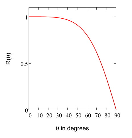
Figure 1: The subluminality factor in Eq. (10) representing the energy flow velocity (in units of $c$) along the propagation axis $z$ in dependence on the inclination angle $\theta$ of the plane waves.

The case $\theta=90^{\circ}$ corresponds to a standing wave where, as it is well known, energy does not flow. More precisely: in this case the plane $(y,z)$ is a node plane outside of which the energy flows back and forth along the $x$ axis in accordance with the time function $U^{2}.$ (For harmonic time dependence, the behavior of the energy flow instantaneous velocity of standing waves has been thoroughly studied, e.g., in Kaiser2011 ). We will see in the following that the obtained ratio $R(\theta)$ of the energy axial velocity to the universal constant $c$ is not peculiar to the given simple model 2D field but holds generally for propagation-invariant fields. Moreover, if we introduce the normalized velocity $\beta\equiv v/c$, we can rewrite Eq. (10) in following two forms:

$$R(\beta)\equiv\frac{2\beta^{-1}}{\beta^{-2}+1}=\frac{2\beta}{\beta^{2}+1}~{}.$$ (11)

The last equality is remarkable and we shall comment on it in the discussion provided in Sec. VI.

In order to get an idea about the energy velocity vectors outside of the axial region, the velocity field is depicted in Fig. 2 for the case of the pulse wavefunction $U$ comprised of a single positive half-period of a cosine. Outside the crossing region the energy flows perpendicularly to the pulse front with velocity $c$ as expected. In the central region, the pulses sum up resulting in almost a 4-fold (if the angle $\theta$ is small) increase of both the energy flux density and the energy density, while the ratio of these two quantities—the energy velocity—is smaler than $c$. Since the horizontal axis of Fig. 2 represents the propagation variable $\zeta\equiv z\cos\theta-ct$, the plots can be interpreted either as ”snapshots in flight” made at a fixed value of time $t$, or as plots on the $(-t,x)$-plane made at a fixed value of the coordinate $z$. From the latter interpretation it follows immediately that for all spatial points, except for those on the $z$ axis, the $x$-component of the Poynting vector as well as $V_{x}$ reverse their sign with increasing of time. In contrast, $S_{z}$ and $V_{z}$ remain non-negative for all values of $x$, $z$, and $t$.

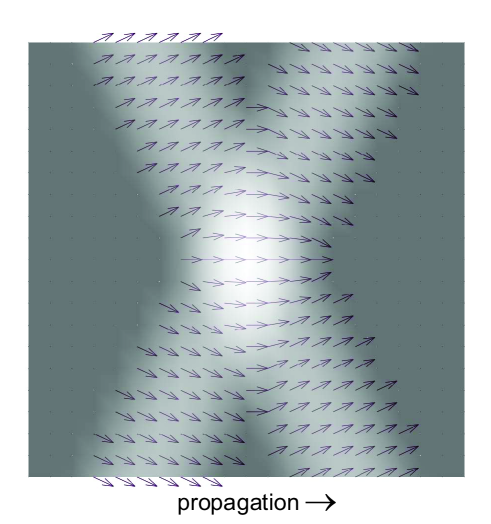
Figure 2: The field of energy flow velocities formed by the crossing of two unipolar half-cycle pulses, depicted by arrows on a grid of $21\times 21$ points. The length of arrows represents the magnitude of the vectors, which equals to $c$ on the branches of the X-profile and is smaller than $c$ on the $z$ axis according to Eq. (10). The $x$ axis is vertical. The horizontal axis represents the propagation variable $z\cos\theta-ct$. For $\theta=25^{\circ}$, the energy velocity on the axis $z$ is $V_{z}\equiv V=0.99518$ in accordance with Eq. (10). The vector field plot is superimposed by a semitransparent greyscale surface (grid $21\times 21$) plot of the square root of the energy density distribution. The velocity vectors are shown only for regions where the energy density exceeds 0.1% of its maximum value.

In Fig. 3, the velocity field is depicted for the case where the pulse wavefunction $U$ comprises a cosine in the interval from $-3\pi/2$ to $3\pi/2$. We see an embryonic pattern of interference between crossing harmonic plane waves. While the velocity equals to $c$ and is directed perpendicularly to the X-branches outside of the interference region, it is much smaller and points in various directions in regions of destructive interference. Other features are the same as in Fig. 2.

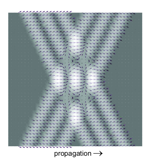
Figure 3: The field of energy flow velocities and the square root of the energy density distribution formed by the crossing of two bipolar 1.5-cycle pulses. The grid of   the plots consists of $41\times 41$ points. For other characteristics see caption of Fig. 2.

Despite the rather coarse grid, Fig. 3 indicates some subtleties in the behavior of the energy velocity at locations of minima of the energy density in the case when the function $U$ contains an oscillating factor. A detailed numerical and analytical study with $U$ taken as a sine or cosine function reveals the following: (i) on a line $\zeta=\zeta_{0}$ corresponding to a zero of the sine or cosine, the Poynting vector vanishes identically for all values of $x$ in the region of interference of the two waves, while the energy density is nonzero, except for the value $x=0$; (ii) the local energy velocity is zero in such planes, except at the points on the $z$ axis where Eq. (10) holds as it does generally on the $z$ axis; (iii) at the points $(\zeta=\zeta_{0},x=0)$ the velocity makes a jump between zero and the value given by Eq. (10); (iv) which of the two values the velocity takes depend on the order in taking the double limit $\zeta\rightarrow\zeta_{0},x\rightarrow 0$. Although such a discontinuity is unphysical, it is not a serious problem, since the energy density vanishes at the discontinuity points and the velocity is therefore undefined in a physical sense anyway (mathematically there is the $0/0$-uncertainty).

III.2 Generalization to 3D cylindrical fields

Although propagation-invariant light sheets have become a subject of intensive study recently, as mentioned in the Introduction, 3D counterparts of them, in particular cylindrically symmetric ones, have been of main interest. One of the reasons is that the energy density in the central spot of a monochromatic $J_{0}$-Bessel beam, as well as in the apex of the double-conical profile of a X-type pulse, exceeds considerably (more than four times) the energy density outside the center, which further decreases inversely proportionally with the distance from the propagation axis.

Do the relations Eq. (10) or Eq. (11) also hold for 3D propagation-invariant fields? The latter can be considered as summing up the pairs of plane waves considered in the previous subsection whereas the axis $x$ there takes all values of the azimuthal angle $\phi$ $\in\left[0\ldots\pi\right]$ around the axis $z$. Since the quantities $S$ and $w$ are not linear with respect to fields $\mathbf{E}$ and $\mathbf{B}$, it is far from being obvious that the expressions Eq. (8)-(9) hold also for such a cylindrically symmetric superposition of the fields. On the $z$ axis the EM fields of a pair of plane waves considered above are given by

$$\mathbf{E}_{p}(x,z,t)|_{x=0} =2\cos\theta\,U(z\cos\theta-ct)\mathbf{e}_{x}\ ,$$

$$\mathbf{B}_{p}(x,z,t)|_{x=0} =2c^{-1}U(z\cos\theta-ct)\mathbf{e}_{y}\ .$$

Let us now take another such pair for which the axis $$x \phi z 3\times 3 T(\phi) 1/2 \frac{1}{2}\left[1\mathbf{+}T(\phi)\right]\mathbf{E}_{p} \frac{1}{2}\left[1\mathbf{+}T(\phi)\right]\mathbf{B}_{p} (\cos\phi+1) V U R(\theta) T(\phi)\mathbf{E}_{p} T(\phi)\mathbf{B}_{p} \phi \left[0\ldots\pi\right] 4 R(\theta) \theta.$$ is rotated by an angle around the axis . If we denote the corresponding coordinate transformation matrix by , we can express the -weighted sum of the fields of the two pairs as , and calculate the flux and energy density. The resulting expressions turn out to be the same as Eqs. (8) and (9) but both multiplied by a factor which cancels out from the expression of . As in the case of obtaining Eq. (10), the square of the function also cancels out from the ratio of the energy flux and density. Thus, Eq. (10), with the subluminality factor , remains valid for the resultant field of two or more pairs of plane waves irrespective of the azimuthal angles between their directions. Likewise, for a rotationally symmetric superposition of the pairs, one has to integrate and over in the interval and calculate the flux and energy density in the resultant fields. The results coincide with Eqs. (8) and (9) multiplied by . Hence, the factor given by Eq. (10) expresses also in the case of rotationally symmetric propagation-invariant 3D waves the dependence of the energy flow velocity along the propagation axis on the Axicon angle

IV Energy flow velocity of superluminal propagation-invariant electromagnetic and scalar fields

IV.1 Fields with fixed value of Axicon angle

It is interesting first to verify whether the formula in Eq. (10) or Eq. (11) holds in the case of the best known superluminal fields—Bessel beams, Bessel-X and X-waves, where not only the intensity or energy density but also the field itself is propagation-invariant. All these comprise cylindrically symmetric superpositions of plane waves directed at a fixed angle $\theta$ with respect to axis $z$ and differ only by the temporal wave profile $U$. The function $U$ contains, respectively, infinitely many (Bessel beam) or few cycles (Bessel-X) or a single unipolar Lorentzian-like pulse (X-wave) and cancels out in the ratio of energy flux and density. Therefore the energy velocity on the propagation axis (i.e., where $\rho\equiv\sqrt{x^{2}+y^{2}}=0)$ of all these waves should be given by Eq. (10) or Eq. (11).

Expressions for the time-averaged Poynting vector and energy density for electromagnetic Bessel beams of the zeroth order can be found in Ari1993 . Examination of the complicated Eq. (44) (for $\mathbf{S}$) and Eq. (43) (for $w$) derived there for a plane-polarized $\mathbf{E}$, bearing in mind that the ratio $\beta/k$ is equal to our $\cos\theta$, shows that on the axis the ratio $\mathbf{S}/w$ indeed turns out to be same as our Eq. (10). Examination of Eq. (51) (for $w$) and Eq. (52) (for $\mathbf{S}$) derived there for the case of a circularly polarized Bessel beam results in the same conclusion. In the last case of polarization the authors of Ref. Ari1993 have found that at the radial distances from the $z$ axis which correspond to the zeros of the Bessel function, the $z$-component of the Poynting vector assumes slightly negative values. Since it means also negative values of $V_{z}$, for the sake of comparison we carried out calculations of the time-averaged Poynting vector, energy density and velocity of TM Bessel beams obtained with the Hertz vector, whose $z$-component is given by a scalar Bessel beam field of arbitrary order $m$. Our results are the following: (i) the $z$-component of the velocity does not assume negative values at any radial distance $\rho$ from the $z$-axis; (ii) as $\rho$ increases the velocity oscillates (in accordance with the behavior of the Bessel function) while the maximum values are given by Eq. (10); (iii) for $m>0$ the first maximum is at $\rho=0$, i.e., the formula Eq. (10 holds on the $z$-axis, while for $m=0$ the velocity is zero on the $z$-axis.

The Poynting vector and energy density for electromagnetic fields derived from a Hertz potential given by a scalar ultrabroadband X-shaped wave, first derived in Lu-X ; Zio1993 ], were calculated in Recami1998 , see Eq. (6) therein. Again, the angular dependence of the ratio of the two quantities coincides with our Eq. (10). However, since the EM field vectors are obtained from Hertz potentials through spatial and temporal derivatives, the central maximum of the X-shaped Hertz potential turns into zero values for some field components, as well as the Poynting vector, on the $z$ axis. In contrast, the first-order scalar ultrabroadband X-wave, which is azimuthally asymmetric (has a factor $\exp i\varphi$), is zero in the center. In this case the axial component of the Poynting vector does not vanish in the center of the pulse as one can see from Eq. (14) of Ref. Salem2011 where the Poynting vector of such X-wave has been calculated for a general (TM+TE) polarization.

In order to clarify when our formula in Eq. (10 or Eq. (11 holds and when not, we calculated the energy velocity for different EM-fields derived from X-shaped Hertz potentials. Without loss of generality, we restricted ourselves to the TM field case. The results are the following.

1. In the case of the azimuthally symmetric scalar potential $\psi_{x}\left(\rho,z,t\right)$ given in Eq. (4), the local energy flow velocity turns out to be zero at the center of the pulse, but in the central cross-sectional plane it increases with the distance from the $z$ axis and approaches its maximum on a ring of radius $\rho=\sqrt{2}a$, where the formula in Eq. (10) holds. Such a behavior is similar to that of the case of the Bessel beam of order $m=0$ described above.

2. In the case of the azimuthally asymmetric scalar potential given by $\psi_{x}^{as}\left(\rho,z,\varphi,t\right)=\psi_{x}\left(\rho,z,t\right)^{3}\rho\exp(i\varphi)$, the formula in Eq. (10) holds at the center of the pulse, as well as on a ring of radius $\rho=2a$, where its second maximum is located.

3. In the case of the azimuthally asymmetric scalar potential used to form the Hertz vector in Salem2011 , the formula in Eq. (10) holds at the center of the pulse. The same holds for another azimuthally asymmetric scalar potential taken for the Hertz vector in Recami1998 .

IV.2 Fields with frequency-dependent Axicon angle

Not all non-diffracting fields can be represented as angular superpositions of plane wave pulses as shown earlier, or—in the case of spectral representation of cylindrical fields—as superpositions of monochromatic Bessel beams whose axial wavenumbers are proportional to the frequency. More general non-diffracting fields, where not the field itself but only its intensity (energy flux and/or density) is propagation-invariant, can be represented as angular superpositions of tilted pulses or—in spectral terms—as superpositions of Bessel beams where the axial wavenumber depends linearly but not simply proportionally on the frequency (see, e.g., LWI ; meieLWIs ; MeieLorTr ). This means that the angle $\theta$ is not fixed any more and becomes a function of frequency within the spectral band of the pulse.

Since (i) directed optical EM fields are in good approximation describable as scalar fields and (ii) there are many studies of scalar non-diffracting fields in the literature but few studies of their EM counterparts, in what follows we deal primarily with the energy velocity of scalar fields. However, first we must answer the question to what extent is the scalar treatment justified in calculations of the energy velocity. It is easy to check that in the case of a pair of scalar plane waves (light sheets), the same expressions for the axial velocity given in Eqs. (10) and (11) follow from Eq. (3).

Since a single-frequency Bessel beam is the constituent of all cylindrical non-diffracting pulses, we carried out numerically comparisons between energy velocity fields of a scalar Bessel beam and vectorial (EM) Bessel beams OttMag ; PIERS2013 The main result is that the velocity field calculated using the scalar approximation practically coincides with those calculated for EM Bessel beams of different polarizations, except for small off-axis regions around minima of energy density, where the discrepancy is about a few percent of $c$ if $\theta<20^{\circ}$ and much less at paraxial values of $\theta$.

Bessel beams considered so far have infinite aperture and therefore cannot be generated in reality. To check that Eq. (10 works also with realistic Bessel beams, we applied Eq. (3) to a so-called Bessel-Gauss beam (see PorrBessGauss and Refs. therein), which is a cylindrically symmetric superposition of Gaussian beams propagating under the Axicon angle $\theta$ with respect to the $z$ axis and have a superluminal group velocity in the waist region. Our result is that Eq. (10) holds if $\theta<15^{\circ}$ which is understandable since the Bessel-Gauss beam is a solution of the paraxial wave equation.

The first example of a superluminal scalar field with frequency-dependent Axicon angle is the so-called Focused X Wave (FXW) revPIER , possibilities of optical generation of which have been considered in Ref. meieFXW . The expression for the FXW reads

$$\psi_{fxw}\left(\rho,z,t\right) =\psi_{x}\left(\rho,z,t\right)\times$$

$$\exp\left[\frac{-|k|}{\psi_{x}\left(\rho,z,t\right)}\right]\exp\left[ik\tilde{\gamma}\frac{v}{c}\left(z-\frac{c^{2}}{v}t\right)\right]~{},$$

where $\psi_{x}$ had been defined by Eq. (4) and $k$ is a new parameter—the smallest wavenumber in the spectrum of the pulse. Obviously $\psi_{fxw}\left(\rho,z,t\right)\rightarrow\psi_{x}\left(\rho,z,t\right)$ if $k\rightarrow 0$. Due to the second exponential factor, $\psi_{fxw}$ is not propagation-invariant, while its modulus squared is.  The energy flow velocity $V_{z}$ along the $z$-direction evaluated with Eq. (3), that is maximum at $\rho=0$, does not obey Eq. (11): in addition to $v$, it depends on $k$ and $a$, but, interestingly, not on $vt$ arising from the second (subluminal) speed. For relatively small values of the parameter $a$ and superluminal values of $v$ close to $c$ Eq. (11) holds for values of $k$ up to 5 (in reciprocal units of $z,\rho,$ and $a$).

Essentially, the same behavior applies for the energy velocity of the vector-valued (TM) FXW. In this case however, $V_{z}$ is equal to zero at $\rho=0$; its maximum value occurs for a value of $\rho>0$. Also, in addition to $k$, the solution is sensitive to $vt$.

All fields considered so far have infinite total energy, i.e., in reality they can exist only within a limited aperture. It is interesting to consider the so-called Modified Focused X wave (MFXW) which has finite energy and is given by revPIER

$$\psi_{mfxw}\left(\rho,z,t\right) =\psi_{x}\left(\rho,z,t\right)\times$$

$$\left[\psi_{x}^{-1}\left(\rho,z,t\right)+a^{\prime}-i\tilde{\gamma}\frac{v}{c}\left(z-\frac{c^{2}}{v}t\right)\right]^{-1}~{},$$

where $a^{\prime}$ is the second width parameter. Again, $V_{z}$, that is maximum at $\rho=0$, does not obey Eq. (11) but depends on $v,a,a^{\prime}$, and $vt$.  For relatively small values of the parameter $a$, relatively large values of $a^{\prime}$ and superluminal values of $v$ close to $c$, the formula Eq. (11) is obeyed very closely because $vt$ appears as a multiplicative factor of $(v^{2}-c^{2})$.

Essentially, the same behavior applies for the energy velocity of a vector-valued MFXW. Again, due to the specific construction of the TM field from the axially oriented Hertz vector potential, in this case $V_{z}$ is equal to zero at $\rho=0$; its maximum value occurs for a value of $\rho>0$.

V Energy flow velocity of subluminal propagation-invariant electromagnetic and scalar fields

It is intriguing to ask: if the energy flows always subluminally in a superluminal pulse, is the flow of the energy of a subluminal pulse faster or slower than its subluminal group velocity?

The best known and simplest subluminal propagation-invariant scalar field is the infinite-energy MacKinnon wave packet MacKinn ; revPIER ; MeieLorTr . It is derived from a spherically symmetric standing wave given by $\exp(-ikct)(\sin kr)/kr$, where $k$ is the wavenumber and $r=\sqrt{\rho^{2}+z^{2}}$, by applying a Lorentz transformation with subluminal $\ \beta=v/c$ to the $z$-coordinate and time. For an observer in another reference frame the field is not any more a monochromatic standing wave, but a pulse whose intensity distribution propagates with velocity $v$ without any change. We found that the formula Eq. (11) holds for the axial energy velocity of the MacKinnon wave packet.

We studied also a finite-energy version of the MacKinnon wave packet given by revPIER

$$\psi_{fM}\left(\rho,z,t\right)=\frac{\arctan\left[\frac{\sqrt{\gamma^{2}\left(z-vt\right)^{2}+\rho^{2}}}{a+i\beta\gamma\left(z-ct/\beta\right)}\right]}{\sqrt{\gamma^{2}\left(z-vt\right)^{2}+\rho^{2}}}~{},$$

where $\gamma\equiv 1/\sqrt{1-(v/c)^{2}}=$ $1/\sqrt{1-\beta^{2}}$ is the common (subluminal) Lorentz factor and $a$ is a parameter. Again, the formula in Eq. (11) holds.

As to the vector-valued version of the MacKinnon wave packet, due to the specific construction of the TM field from the axially oriented Hertz vector potential with the MacKinnon scalar wavepacket as its z-component, $V_{z}$ is equal to zero at $\rho=0$; whereas Eq. (11) holds at its maxima values that occur at values of $\rho$ corresponding to the maxima of the sinc-function.

The last almost-undistorted spatiotemporally localized field we studied was the finite energy azimuthally symmetric subluminal splash mode. It arises from the elementary solution $(\rho^{2}+z^{2}-c^{2}t^{2})^{-1}$ of the scalar wave equation by first resorting to the complexification $t\rightarrow t+ia$ and subsequently undertaking a subluminal Lorentz transformation involving the coordinates $z$ and $t$. A scalar-valued computation yields a maximum axial energy velocity at the pulse center in conformity with the formula in Eq. (11). A vector-valued computation shows that the axial energy velocity is zero on-axis ($\rho=0$) at the pulse center. The maximum value of the axial velocity depends on $vt$ and the parameter $a$. For small values of $vt$ or subluminal speed $v$ very close to $c$ and $a=1$ the maximum of the axial energy flow velocity occurs on a ring of radius $\rho=1$.

Finally we studied a propagation-variant scalar field, which is important for applications and is called ”pulsed Bessel beam” DifRefAxiconBB ; PorrGaussjaPBB Since it is formed by a diffractive axicon (a circular grating), it is like a disk cut off from a Bessel beam— its radial profile is propagation invariant and given by the zeroth-order Bessel function, while its longitudinal profile spreads out in the course of propagation as a chirped pulse. Such behavior has been experimentally studied in detail with $\operatorname{fs}$-range temporal and $\operatorname{\mu m}$-range spatial resolution meieDifAxicon0 ; meieDifAxicon1 .

In the given case, the field to be inserted into Eq. (3) factorizes as $\psi=U(z,t)J_{0}(k_{0}\rho\sin\theta)$, where $k_{0}$ is the carrier wavenumber (mean wavenumber in the spectrum of the pulse). For the field of a pulsed Bessel beam with Gaussian temporal profile, the function $U(z,t)$ was calculated using Eqs. (44), (45) and (54) from Ref. PorrGaussjaPBB . As one can see in Fig. 4, the pulse broadens and gets chirped in the course of propagation. The reason is that waves of different wavenumbers diffract at different angles on the grating, which means that the Axicon angle is not constant over the spectrum of the pulse.

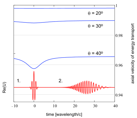
Figure 4: Time dependence of the real part of the function $U(z,t)$ of a pulsed Bessel beam with a mean value of the Axicon angle $\theta=40^{\circ}$ (determined for the carrier wavenumber) and Gaussian temporal profile of width $1$ (in units of carrier wavelength divided by $c$): curve 1 – at the origin $z=0$ where the pulse is formed and has the shortest duration, curve 2 – at $z=20$ (in units of the carrier wavelength). The curves with indicated mean Axicon angles show temporal behavior of the energy velocity (normalized to $c)$ at the maximum of the pulse envelope.

Despite the chirp, locally the pulse looks like a Bessel beam characterized by an instantaneous wavenumber and corresponding Axicon angle. Therefore, based upon the results obtained above, Eq. (10) should hold at time instances and propagation distances when the pulse contains more than just a few cycles. This is exactly what we see in Fig. 4: at small mean angles $\theta$—not speaking about paraxial angles—the energy velocity is almost at a constant level determined by Eq. (10)  The slight drop in its value occurs only at the origin if the pulse is shorter than 2 wavelengths there and $\theta>20^{\circ}$. The drop at such extreme parameters may be caused also by the circumstance that in the calculation of the function $U(z,t)$ in Ref. PorrGaussjaPBB the group velocity dispersion is only approximately taken into account.

To conclude, the answer to the question raised in the beginning of the Section is: in those regions of a subluminal pulse where Eq. (11) holds, the energy flows faster than the pulse envelope, i.e. $0<v<V_{z}=V<c$

VI Discussion

We have seen that—with a few exceptions—the formula given in Eq. (11) holds for the energy axial velocity of both superluminal and subluminal non-diffracting wavefields. Moreover, Eq. (11) indicates that the velocity does not change if one makes a transition superluminal$\longleftrightarrow$subluminal, i.e., replaces the normalized group velocity $\beta=v/c$ by its reciprocal value $c/v$. To understand the reason of such an interesting feature of the expression let us take a look at the expression of the energy velocity in terms of impedance ImpedZ , viz.

$$\mathbf{V} =2c\frac{\mathbf{E}\times c\mathbf{B}}{\mathbf{E}^{2}+c^{2}\mathbf{B}^{2}}=c\frac{2Z}{1+Z^{2}}\left(\mathbf{e}_{E}\times\mathbf{e}_{B}\right)~{},$$ (13)

$$Z \equiv\frac{E}{cB}=\frac{E}{H}Z_{0}^{-1}~{},$$ (14)

where $E$, $B$ are the magnitudes of electric and magnetic field vectors and $\mathbf{e}_{E}$, $\mathbf{e}_{B}$ are corresponding unit vectors; $Z$ is the impedance normalized to the vacuum impedance $Z_{0}=\sqrt{\mu_{0}/\varepsilon_{0}}\approx 377\Omega$. Thus, the group velocity is determined by the impedance $\beta=Z$ and the energy velocity Eq. (13) does not change if we insert $Z^{-1}$ instead of $Z$. This is due to the invariance of the energy flux and energy density with respect to the duality transformation $\mathbf{E}\rightarrow c\mathbf{B}$, $\mathbf{B}\rightarrow-\mathbf{E/}c$ . From the duality also follows that our results obtained for TM pulses apply also for TE pulses. $Z=1$ and, consequently, $V=c$ holds only for TEM and null electromagnetic waves Lekner2002 ; YannisLWII ; Kaiser2011 .

Note also that Eq. (11) resembles the relativistic composition law for velocities. One can speculate that the energy velocity equals the pulse propagation velocity seen from a reference frame countermoving with exactly the pulse group velocity.

It is well known that the Poynting vector is not defined uniquely by the Poynting theorem. Could it be that, consequently, the energy flow velocity we have dealt with throughout this paper is not also defined uniquely and therefore its nonequality to the group velocity would not be of interest? The answer is that any other definition of the Poynting vector might violate the velocity upper limit $c$ Lekner2002 . Here a quotation from Jackson , section 8.5 is appropriate: ”However the theory of special relativity, in which energy and momentum are defined locally and invariantly via the stress–energy tensor, shows that the … expression for the Poynting vector is unique.”

According to conventional thinking, energy should be tightly coupled to an EM field pulse. How, then, one has to interpret the results that energy flows slower than a superluminal pulse itself and flows faster than a subluminal pulse? Nonequality of energy flow velocity to the velocity of field motion is not unique for non-diffracting localized waves but takes place in other non-null fields, e.g., in standing waves, dipole radiation, Kaiser2011 , etc. In Ref. Kaiser2011 this nonequality is explained in terms of reactive (rest) energy that the field leaves behind. In this paper one can also find a hint towards comprehension of this inequality: ”A rough way to understand why $V<c$ is by analogy with water waves. The mass carried by the waves has a definite speed at each point and time, but this need not coincide with the propagation speed of the wavefronts.” Existence of a rest energy portion in non-diffracting localized waves is obvious because all of them contain a standing-wave component. It is interesting to note that the standing wave component inherent to these waves can be given an interpretation as if the mass of a photon of these wavefields is not equal to zero Minupeatykk .

Finally, let us note that the signal velocity of superluminal nondiffracting pulses is not superluminal but an instantaneous notch made, e.g., into Bessel-X pulse, which transforms into the subluminal propagation-variant pulse considered above, as proved by a thought experiment in Ref. Minupeatykk .

VII Conclusions

We have shown that the velocity $V$, with which energy in non-diffracting pulsed waves flows in the direction of propagation, is not equal to the propagation velocity $v$ (group velocity) of the pulse itself. Instead, on the symmetry axis and/or at the locations of the energy density maxima, these two quantities obey a simple but physically content-rich relation $V=2v/\left[1+(v/c)^{2}\right]$. This has been proven first for vector-valued superluminal 2D light sheets and their 3D cylindrical generalizations in Sec. III. Subsequently, it has been shown to be valid for the scalar-valued $m$-order Bessel beam, the fundamental zero-order X wave, the first-order azimuthally asymmetric X wave, as well as the corresponding vector-valued TM electromagnetic fields based on a Hertzian potential approach. The behavior of the axial velocity for the vector-valued fields differs depending on whether the scalar potential used as a seed in forming the vector Hertz potential is azimuthally symmetric or asymmetric. A detailed discussion is provided in Sec. IV.

Purely propagation-invariant fields characterized by the group speed $v$ along the direction of propagation are physically unrealizable. Physically realizable spatiotemporally localized waves contain two speeds: the group speed $v$ (superluminal or subluminal) and a second speed $c^{2}/v$ (subluminal or superluminal). Between the purely propagation-invariant and the physically realizable “almost undistorted” localized waves, there exists a family of only intensity-invariant localized waves containing the aforementioned two speeds. Examples for such pulses are the Focus X Wave (FXW) and MacKinnon’s wave packet. Both are characterized by infinite energy content. The energy flow velocity for these two scalar fields, the scalar finite-energy pulses based on them, as well as the corresponding vector-valued TM electromagnetic fields determined by a Hertzian potential approach obey the universal formula given in Eq. (11) very closely provided the group velocity is very close to the speed of light and certain free parameters are tweaked appropriately. Specific details are given in Secs. III-V.

It is very interesting to note that the universal formula for the axial energy flow velocity, in the form appearing in Eq. (11), is intimately related to the wave impedance reformulation in Eq. (13), which, in turn, is reminiscent of a relativistic expression for the addition of velocities.

Finally, a note on superluminality is appropriate. The presence of a superluminal speed in a finite-energy solution does not contradict relativity. If the parameters are chosen appropriately, the pulse moves superluminally with almost no distortion up to a certain distance $z_{d}$, which is determined by the geometry (aperture size and an axicon angle) and then it slows down to a luminal speed $c$, with significant accompanying distortion. Although the peak of the pulse does move superluminally up to $z_{d}$, it is not causally related at two distinct ranges $z_{1},z_{2}\in[0,z_{d})$. Thus, no information can be transferred superluminally from $z_{1}$ to $z_{2}$. The physical significance of such wavepackets is due to their spatiotemporal localization.

The authors thank Ari Friberg and John Lekner for giving comments to their papers Ari1993 and Lekner2002 , which stimulated undertaking the present study.

Appendix A PROOF OF CONDITION $\left|\mathbf{V}\right|\leq c$ FOR SCALAR FIELDS

Similarly to Eq. (2) we can write by using Eq. (3):

$$1-\frac{\mathbf{V}^{2}}{c^{2}}=1-\frac{1}{c^{2}}\frac{\left(\dot{\psi}^{\ast}\mathbf{\nabla}\psi+\dot{\psi}\mathbf{\nabla}\psi^{\ast}\right)^{2}}{\left(\frac{1}{c^{2}}\dot{\psi}\dot{\psi}^{\ast}+\mathbf{\nabla}\psi\cdot\mathbf{\nabla}\psi^{\ast}\right)^{2}}$$ (15)

This form can be used to prove that $\left|\mathbf{V}\right|\leq c$.  Indeed, making use of the notations $F\equiv\mathbf{\nabla}\psi\cdot\mathbf{\nabla}\psi^{\ast}-\frac{1}{c^{2}}\dot{\psi}\dot{\psi}^{\ast}$ and $\mathbf{G}\equiv\dot{\psi}\mathbf{\nabla}\psi^{\ast}$ for convenience, we can transform Eq. (15) as follows:

$$1-\frac{\mathbf{V}^{2}}{c^{2}} =\frac{F^{2}+\frac{2}{c^{2}}\mathbf{G}\cdot\mathbf{G}^{\ast}-\frac{1}{c^{2}}\left(\mathbf{G}\cdot\mathbf{G}+\mathbf{G}^{\ast}\cdot\mathbf{G}^{\ast}\right)}{\left(\frac{1}{c^{2}}\dot{\psi}\dot{\psi}^{\ast}+\mathbf{\nabla}\psi\cdot\mathbf{\nabla}\psi^{\ast}\right)^{2}}=$$

$$=\frac{F^{2}+\frac{2}{c^{2}}\mathbf{G}\cdot\mathbf{G}^{\ast}+\frac{4}{c^{2}}\left(\operatorname{Im}\mathbf{G}\right)^{2}-\frac{2}{c^{2}}\mathbf{G}\cdot\mathbf{G}^{\ast}}{\left(\frac{1}{c^{2}}\dot{\psi}\dot{\psi}^{\ast}+\mathbf{\nabla}\psi\cdot\mathbf{\nabla}\psi^{\ast}\right)^{2}}$$

$$=\frac{F^{2}+\frac{4}{c^{2}}\left(\operatorname{Im}\mathbf{G}\right)^{2}}{\left(\frac{1}{c^{2}}\dot{\psi}\dot{\psi}^{\ast}+\mathbf{\nabla}\psi\cdot\mathbf{\nabla}\psi^{\ast}\right)^{2}}~{}.$$

The denominator and numerator of the last fraction are nonnegative and, as a consequence, $\left|\mathbf{V}\right|\leq c$.

References

- (1) D. Giovannini, J. Romero, V. Potoček, G. Ferenczi, F. Speirits, S. M. Barnett, D. Faccio, and M. J. Padgett, Spatially structured photons that travel in free space slower than the speed of light, Science 347, 857 (2015).
- (2) Z. L. Horváth and B. Major, Comment on ”Spatially structured photons that travel in free space slower than the speed of light,” arXiv:1504.06059.
- (3) N. D. Bareza and N. Hermosa, Subluminal group velocity and dispersion of Laguerre-Gauss beams in free space, Sci. Rep. 6, 26842 (2016).
- (4) F. Bouchard, J. Harris, H. Mand, R. W. Boyd, and E. Karimi, Observation of subluminal twisted light in vacuum, Optica 3, 351 (2016).
- (5) P. Saari, Observation of subluminal twisted light in vacuum: Comment, Optica 4, 204 (2017).
- (6) R. R. Alfano, and D. A. Nolan, Slowing of Bessel light beam group velocity, Opt. Commun. 361, 25 (2016).
- (7) P. Saari, Comments on “Slowing of Bessel light beam group velocity.” Opt. Commun. 392, 300 (2017).
- (8) T. Roger, A. Lyons, N. Westerberg, S. Vezzoli, C. Maitland, J. Leach, M. Padgett, and D. Faccio, How fast is a twisted photon?, Optica 5, 682 (2018).
- (9) P. Saari, Reexamination of group velocities of structured light pulses, Phys. Rev. A, 97, 063824 (2018).
- (10) H. E. Kondakci and A. F. Abouraddy, Optical space-time wavepackets having arbitrary group velocities in free space, Nature Commun.10, 08735-1-8 (2019).
- (11) B. Bhaduri, M. Yessenov, and A. F. Abouraddy, Space–time wave packets that travel in optical materials at the speed of light in vacuum, Optica 6, 139 (2019).
- (12) R. Smith, The velocities of light, Am. J. Phys. 38, 978 (1970).
- (13) J. Peatross, S. A. Glasgow, and M. Ware, Average energy flow of optical pulses in dispersive media, Phys. Rev. Lett. 84, 2370 (2000).
- (14) P. Milonni, Controlling the speed of light pulses, J. Phys. B: At. Mol. Opt. Phys. 35, R31 (2002).
- (15) Localized Waves, edited by H. E. Hernandez-Figueroa, M. Zamboni-Rached, and E. Recami (J. Wiley, New York, 2007).
- (16) Non-Diffracting Waves, edited by H. E. Hernandez-Figueroa, E. Recami, and M. Zamboni-Rached (J. Wiley, New York, 2013).
- (17) R. Donnelly, and R. Ziolkowski, Designing localized waves, Proc. R. Soc. Lond. A 440, 541 (1993).
- (18) I. Besieris, M. Abdel-Rahman, A. Shaarawi, and A. Chatzipetros, Two fundamental representations of localized pulse solutions to the scalar wave equation, Progr. in Electrom. Res. 19, 1 (1998).
- (19) J. Salo, J. Fagerholm, A. T. Friberg, and M. M. Salomaa, Unified description of nondiffracting X and Y waves, Phys. Rev. E, 62, 4261 (2000).
- (20) P. Saari and K. Reivelt, Generation and classification of localized waves by Lorentz transformations in Fourier space, Phys. Rev. E 69, 036612 (2004).
- (21) A. P. Kiselev, Localized light waves: paraxial and exact solutions of the wave equation (a Review), Optics and Spectroscopy 102, 603 (2007).
- (22) M. Yessenov, B. Bhaduri, H. E. Kondakci, and A. F. Abouraddy, Classification of propagation-invariant space-time wave packets in free space: theory and experiments, Phys. Rev. A 99, 023856 (2019).
- (23) P. Saari and K. Reivelt, Evidence of X-shaped propagation-invariant localized light waves, Phys. Rev. Lett. 79, 4135 (1997).
- (24) J. Durnin, J.J. Miceli, and J.H. Eberly, Diffraction-free beams, Phys. Rev. Lett. 58, 1499 (1987).
- (25) I. Alexeev, K. Y. Kim, and H. M. Milchberg, Measurement of the superluminal group velocity of an ultrashort Bessel beam pulse, Phys. Rev. Lett. 88, 073901 (2002).
- (26) R. Grunwald, V. Kebbel, U. Griebner, U. Neumann, A. Kummrow, M. Rini, E. T. J. Nibbering, M. Piché, G. Rousseau, and M. Fortin, Generation and characterization of spatially and temporally localized few-cycle optical wave packets, Phys. Rev. A 67, 063820 (2003).
- (27) P. Bowlan, H. Valtna-Lukner, M. Lõhmus, P. Piksarv, P. Saari, and R. Trebino, Measurement of the spatio-temporal field of ultrashort Bessel-X pulses,” Opt. Lett., 34, 2276 (2009).
- (28) P. Bowlan, H. Valtna-Lukner, M. Lõhmus, P. Piksarv, P. Saari, and R. Trebino, Measurement of the spatiotemporal electric field of ultrashort superluminal Bessel-X pulses,” Optics and Photonics News 20, 42 (2009).
- (29) H. E. Kondakci and A. F. Abouraddy, Diffraction-free space–time light sheets, Nature Photonics 11, 733 (2017).
- (30) J. D. Jackson, Classical Electrodynamics, 2nd ed. (New York: Wiley 1975).
- (31) J. Lekner, Phase and transport velocities in particle and electromagnetic beams, J. Opt. A: Pure Appl. Opt. 4, 491 (2002).
- (32) I. M. Besieris and A.M. Shaarawi, Spatiotemporally localized null electromagnetic waves I. Luminal, Progress in Electromagnetic Research (PIER) B 8, 1 (2008).
- (33) I. M. Besieris and A. M. Shaarawi, Spatiotemporally localized null electromagnetic waves, in LW2 , p. 161.
- (34) E. Recami, On localized ”X-shaped” superluminal solutions to Maxwell equations, Physica A 252, 586 (1998).
- (35) A. Lotti, A. Couairon, D. Faccio, and P. Di Trapani, Energy-flux characterization of conical and space-time coupled wave packets, Phys. Rev. A 81, 023810 (2010).
- (36) M. A. Salem and H. Bağcı, Energy flow characteristics of vector X-waves, Opt. Express, 19, 8526 (2011).
- (37) D. Mugnai and I. Mochi, Superluminal X-wave propagation: energy localization and velocity, Phys. Rev. E 73, 016606 (2005).
- (38) O. Rebane, The energy transport and signal velocities of localized waves, MSc thesis (University of Tartu, 2011).
- (39) P. Saari, O. Rebane, and I. M. Besieris, Energy transport velocity for various localized and accelerating pulsed waves, in Final Program (with PIERS Abstracts) of Progress In Electromagnetics Research Symposium, Stockholm 2013, p. 40.
- (40) G. Kaiser. Electromagnetic inertia, reactive energy and energy flow velocity, J. Phys. A: Math. Theor. 44, 345206 (2011).
- (41) H. E. Kondakci and A. F. Abouraddy, Self-healing of space-time light sheets, Opt. Lett. 43, 30-3832 (2018).
- (42) I. Bialynicki-Birula and Z. Bialynicki-Birula, Vortex lines of the electromagnetic field, Phys. Rev. A 67, 062114 (2003).
- (43) L. Mandel and E. Wolf, Optical Coherence and Quantum Optics (Cambridge University Press, 1955), p. 288.
- (44) J. Y. Lu, and J. F. Greenleaf, Nondiffracting X waves—Exact solutions to free space scalar wave equations and their aperture realizations, IEEE Trans. Ultrason. Ferroelec. Freq. Contr. 39, 19 (1992).
- (45) R. W. Ziolkowski, I. M. Besieris, and A. M. Shaarawi, Aperture realizations of the exact solutions to homogeneous-wave equations, J. Opt. Soc. Am. A 10, 75 (1993).
- (46) J. Turunen and A. T. Friberg, Self-imaging and propagation-invariance in electromagnetic fields, Pure. Appl. Opt. 2, 51 (1993).
- (47) K. Reivelt and P. Saari, Linear-optical generation of localized waves, in LWI p. 185.
- (48) M. A. Porras, R. Borghi, and M. Santarsiero, Few-optical-cycle Bessel-Gauss pulsed beams in free space, Phys. Rev. E 62, 5729 (2000).
- (49) H. Valtna, K. Reivelt, and P. Saari, Methods for generating wideband localized waves of superluminal group velocity, Opt. Comm. 278, 1 (2007).
- (50) L. A. Mackinnon, A nondispersive de Broglie wave packet, Found. Phys. 8, 157 (1978).
- (51) A. Shaarawi and I. M. Besieris, On the superluminal propagation of X-shaped localized waves. J. Phys. A: Math. Gen., 33, 7227 (2000).
- (52) M. A. Porras, Diffraction effects in few-cycle optical pulses, Phys. Rev. E 65, 026606 (2002).
- (53) M. Lõhmus, P. Bowlan, P. Piksarv, H. Valtna-Lukner, R. Trebino, and P. Saari, Diffraction of ultrashort optical pulses from circularly symmetric binary phase gratings, Opt. Lett., 37, 1238 (2012).
- (54) P. Piksarv, H. Valtna-Lukner, A. Valdman, M. Lõhmus, R. Matt, P. Saari, Temporal focusing of ultrashort pulsed Bessel beams into Airy–Bessel light bullets, Opt. Express, 20, 17220 (2012).
- (55) H. G. Schantz, Energy velocity and reactive fields, Phil. Trans. R. Soc. A 376, 20170453 (2018).
- (56) P. Saari, X-type waves in ultrafast optics, in LW2 p. 109.