Scalable Verification of Probabilistic Networks

Abstract.

This paper presents McNetKAT, a scalable tool for verifying probabilistic network programs. McNetKAT is based on a new semantics for the guarded and history-free fragment of Probabilistic NetKAT in terms of finite-state, absorbing Markov chains. This view allows the semantics of all programs to be computed exactly, enabling construction of an automatic verification tool. Domain-specific optimizations and a parallelizing backend enable McNetKAT to analyze networks with thousands of nodes, automatically reasoning about general properties such as probabilistic program equivalence and refinement, as well as networking properties such as resilience to failures. We evaluate McNetKAT’s scalability using real-world topologies, compare its performance against state-of-the-art tools, and develop an extended case study on a recently proposed data center network design.

1. Introduction

Networks are among the most complex and critical computing systems used today. Researchers have long sought to develop automated techniques for modeling and analyzing network behavior (Xie et al., 2005), but only over the last decade has programming language methodology been brought to bear on the problem (McKeown et al., 2008; Casado et al., 2014; Bosshart et al., 2014), opening up new avenues for reasoning about networks in a rigorous and principled way (Khurshid et al., 2012; Kazemian et al., 2012; Anderson et al., 2014; Foster et al., 2015; Liu et al., 2018). Building on these initial advances, researchers have begun to target more sophisticated networks that exhibit richer phenomena. In particular, there is renewed interest in randomization as a tool for designing protocols and modeling behaviors that arise in large-scale systems—from uncertainty about the inputs, to expected load, to likelihood of device and link failures.

Although programming languages for describing randomized networks exist (Foster et al., 2016; Gehr et al., 2018b), support for automated reasoning remains limited. Even basic properties require quantitative reasoning in the probabilistic setting, and seemingly simple programs can generate complex distributions. Whereas state-of-the-art tools can easily handle deterministic networks with hundreds of thousands of nodes, probabilistic tools are currently orders of magnitude behind.

This paper presents McNetKAT, a new tool for reasoning about probabilistic network programs written in the guarded and history-free fragment of Probabilistic NetKAT (ProbNetKAT) (Anderson et al., 2014; Foster et al., 2015; Smolka et al., 2017; Foster et al., 2016). ProbNetKAT is an expressive programming language based on Kleene Algebra with Tests, capable of modeling a variety of probabilistic behaviors and properties including randomized routing (Valiant, 1982; Kumar et al., 2018), uncertainty about demands (Roy et al., 2015), and failures (Gill et al., 2011). The history-free fragment restricts the language semantics to input-output behavior rather than tracking paths, and the guarded fragment provides conditionals and while loops rather than union and iteration operators. Although the fragment we consider is a restriction of the full language, it is still expressive enough to encode a wide range of practical networking models. Existing deterministic tools, such as Anteater (Mai et al., 2011), HSA (Kazemian et al., 2012), and Veriflow (Khurshid et al., 2012), also use guarded and history-free models.

To enable automated reasoning, we first reformulate the semantics of ProbNetKAT in terms of finite state Markov chains. We introduce a big-step semantics that models programs as Markov chains that transition from input to output in a single step, using an auxiliary small-step semantics to compute the closed-form solution for the semantics of the iteration operator. We prove that the Markov chain semantics coincides with the domain-theoretic semantics for ProbNetKAT developed in previous work (Smolka et al., 2017; Foster et al., 2016). Our new semantics also has a key benefit: the limiting distribution of the resulting Markov chains can be computed exactly in closed form, yielding a concise representation that can be used as the basis for building a practical tool.

We have implemented McNetKAT in an OCaml prototype that takes a ProbNetKAT program as input and produces a stochastic matrix that models its semantics in a finite and explicit form. McNetKAT uses the UMFPACK linear algebra library as a back-end solver to efficiently compute limiting distributions (Davis, 2004), and exploits algebraic properties to automatically parallelize the computation across multiple machines. To facilitate comparisons with other tools, we also developed a back-end based on PRISM (Kwiatkowska et al., 2011a).

To evaluate the scalability of McNetKAT, we conducted experiments on realistic topologies, routing schemes, and properties. Our results show that McNetKAT scales to networks with thousands of switches, and performs orders of magnitude better than a state-of-the-art tool based on general-purpose symbolic inference (Gehr et al., 2018b; Gehr et al., 2016). We also used McNetKAT to carry out a case study of the resilience of a fault-tolerant data center design proposed by Liu et al. (2013).

Contributions and outline.

The central contribution of this paper is the development of a scalable probabilistic network verification tool. We develop a new, tractable semantics that is sound with respect to ProbNetKAT’s original denotational model. We present a prototype implementation and evaluate it on a variety of scenarios drawn from real-world networks. In Section 2, we introduce ProbNetKAT using a running example. In Section 3, we present a semantics based on finite stochastic matrices and show that it fully characterizes the behavior of ProbNetKAT programs (Theorem 3.1). In Section 4, we show how to compute the matrix associated with iteration in closed form. In Section 5, we discuss our implementation, including symbolic data structures and optimizations that are needed to handle the large state space efficiently. In Section 6, we evaluate the scalability of McNetKAT on a common data center design and compare its performance against state-of-the-art probabilistic tools. In Section 7, we present a case study using McNetKAT to analyze resilience in the presence of link failures. We survey related work in Section 8 and conclude in Section 9. We defer proofs to the appendix.

2. Overview

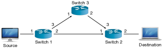
Figure 1. Network topology for running example.

This section introduces a running example that illustrates the main features of the ProbNetKAT language as well as some quantitative network properties that arise in practice.

Background on ProbNetKAT.

Consider the network in Figure 1, which connects a source to a destination in a topology with three switches. We will first introduce a program that forwards packets from the source to the destination, and then verify that it correctly implements the desired behavior. Next, we will show how to enrich our program to model the possibility of link failures, and develop a fault-tolerant forwarding scheme that automatically routes around failures. Using a quantitative version of program refinement, we will show that the fault-tolerant program is indeed more resilient than the initial program. Finally, we will show how to compute the expected degree of resilience analytically.

To a first approximation, a ProbNetKAT program can be thought of as a randomized function that maps input packets to sets of output packets. Packets are modeled as records, with fields for standard headers—such as the source (src) and destination (dst) addresses—as well as two fields switch (sw) and port (pt) encoding the current location of the packet. ProbNetKAT provides several primitives for manipulating packets: a modification $\mathit{f}\kern 0.43057pt{\shortleftarrow}\kern 0.43057ptn$ returns the input packet with field $\mathit{f}$ updated to $n$, while a test $\mathit{f}\kern 0.43057pt{=}\kern 0.43057ptn$ returns either the input packet unmodified if the test succeeds, or the empty set if the test fails. The primitives $\mathsf{skip}$ and $\mathsf{drop}$ behave like a test that always succeeds and fails, respectively. In the guarded fragment of the language, programs can be composed sequentially ($p\mathop{;}q$), using conditionals ($\boldsymbol{\mathsf{if}}~{}p~{}\boldsymbol{\mathsf{then}}~{}q_{1}~{}\boldsymbol{\mathsf{else}}~{}q_{2}$), while loops ($\boldsymbol{\mathsf{while}}~{}p~{}\boldsymbol{\mathsf{do}}~{}q$), or probabilistic choice ($p\oplus q$).

Although ProbNetKAT programs can be freely constructed by composing primitive operations, a typical network model is expressed using two programs: a forwarding program (sometimes called a policy) and a link program (sometimes called a topology). The forwarding program describes how packets are transformed locally by the switches at each hop. In our running example, to route packets from the source to the destination, switches $1$ and $2$ can simply forward all incoming packets out on port $2$ by modifying the port field (pt). This program can be encoded in ProbNetKAT by performing a case analysis on the location of the input packet, and then setting the port field to $2$:

$$p\mathrel{\smash{\triangleq}}{} \boldsymbol{\mathsf{if}}~{}\texttt{sw}\kern 0.43057pt{=}\kern 0.43057pt1~{}\boldsymbol{\mathsf{then}}~{}\texttt{pt}\kern 0.43057pt{\shortleftarrow}\kern 0.43057pt2~{}\boldsymbol{\mathsf{else}}~{}$$

$$\boldsymbol{\mathsf{if}}~{}\texttt{sw}\kern 0.43057pt{=}\kern 0.43057pt2~{}\boldsymbol{\mathsf{then}}~{}\texttt{pt}\kern 0.43057pt{\shortleftarrow}\kern 0.43057pt2~{}\boldsymbol{\mathsf{else}}~{}\mathsf{drop}$$

The final $\mathsf{drop}$ at the end of this program encodes the policy for switch 3, which is unreachable.

We can model the topology as a cascade of conditionals that match packets at the end of each link and update their locations to the link’s destination:

$$t \mathrel{\smash{\triangleq}}\boldsymbol{\mathsf{if}}~{}\texttt{sw}\kern 0.43057pt{=}\kern 0.43057pt1\mathop{;}\texttt{pt}\kern 0.43057pt{=}\kern 0.43057pt2~{}\boldsymbol{\mathsf{then}}~{}\texttt{sw}\kern 0.43057pt{\shortleftarrow}\kern 0.43057pt2\mathop{;}\texttt{pt}\kern 0.43057pt{\shortleftarrow}\kern 0.43057pt1~{}\boldsymbol{\mathsf{else}}~{}\dots$$

To build the overall network model, we first define predicates for the ingress and egress locations,

$$\mathit{in}\mathrel{\smash{\triangleq}}\texttt{sw}\kern 0.43057pt{=}\kern 0.43057pt1\mathop{;}\texttt{pt}\kern 0.43057pt{=}\kern 0.43057pt1 \mathit{out}\mathrel{\smash{\triangleq}}\texttt{sw}\kern 0.43057pt{=}\kern 0.43057pt2\mathop{;}\texttt{pt}\kern 0.43057pt{=}\kern 0.43057pt2$$

and then combine the forwarding policy $p$ with the topology $t$. More specifically, a packet traversing the network starts at an ingress and is repeatedly processed by switches and links until it reaches an egress:

$$\operatorname{M}(p,t)\mathrel{\smash{\triangleq}}in\mathop{;}p\mathop{;}\boldsymbol{\mathsf{while}}~{}\neg\mathit{out}~{}\boldsymbol{\mathsf{do}}~{}(t\mathop{;}p)$$

We can now state and prove properties about the network by reasoning about this model. For instance, the following equivalence states that $p$ forwards all packets to the destination:

$$\operatorname{M}(p,t)\ \equiv\ in\mathop{;}\texttt{sw}\kern 0.43057pt{\shortleftarrow}\kern 0.43057pt2\mathop{;}\texttt{pt}\kern 0.43057pt{\shortleftarrow}\kern 0.43057pt2$$

The program on the right can be regarded as an ideal specification that “teleports” each packet to its destination. Such equations were also used in previous work to reason about properties such as waypointing, reachability, isolation, and loop freedom (Anderson et al., 2014; Foster et al., 2015).

Probabilistic reasoning.

Real-world networks often exhibit nondeterministic behaviors such as fault tolerant routing schemes to handle unexpected failures (Liu et al., 2013) and randomized algorithms to balance load across multiple paths (Kumar et al., 2018). Verifying that networks behave as expected in these more complicated scenarios requires a form of probabilistic reasoning, but most state-of-the-art network verification tools model only deterministic behaviors (Khurshid et al., 2012; Kazemian et al., 2012; Foster et al., 2015).

To illustrate, suppose we want to extend our example with link failures. Most modern switches execute low-level protocols such as Bidirectional Forwarding Detection (BFD) that compute real-time health information about the link connected to each physical port (Bhatia et al., 2014). We can enrich our model so that each switch has a boolean flag $\texttt{up}_{i}$ that indicates whether the link connected to the switch at port $i$ is up. Then, we can adjust the forwarding logic to use backup paths when the link is down: for switch $1$,

$$\widehat{p}_{1}\mathrel{\smash{\triangleq}}{} \boldsymbol{\mathsf{if}}~{}\texttt{up}_{2}\kern 0.43057pt{=}\kern 0.43057pt1~{}\boldsymbol{\mathsf{then}}~{}\texttt{pt}\kern 0.43057pt{\shortleftarrow}\kern 0.43057pt2~{}\boldsymbol{\mathsf{else}}~{}$$

$$\boldsymbol{\mathsf{if}}~{}\texttt{up}_{2}\kern 0.43057pt{=}\kern 0.43057pt0~{}\boldsymbol{\mathsf{then}}~{}\texttt{pt}\kern 0.43057pt{\shortleftarrow}\kern 0.43057pt3~{}\boldsymbol{\mathsf{else}}~{}\mathsf{drop}$$

and similarly for switches $2$ and $3$. As before, we can package the forwarding logic for all switches into a single program:

$$\widehat{p} \mathrel{\smash{\triangleq}}\boldsymbol{\mathsf{if}}~{}\texttt{sw}\kern 0.43057pt{=}\kern 0.43057pt1~{}\boldsymbol{\mathsf{then}}~{}\widehat{p_{1}}~{}\boldsymbol{\mathsf{else}}~{}\boldsymbol{\mathsf{if}}~{}\texttt{sw}\kern 0.43057pt{=}\kern 0.43057pt2~{}\boldsymbol{\mathsf{then}}~{}\widehat{p_{2}}~{}\boldsymbol{\mathsf{else}}~{}\widehat{p_{3}}$$

Next, we update the encoding of our topology to faithfully model link failures. Links can fail for a wide variety of reasons, including human errors, fiber cuts, and hardware faults. A natural way to model such failures is with a probabilistic model—i.e., with a distribution that captures how often certain links fail:

$$f_{0} \mathrel{\smash{\triangleq}}\texttt{up}_{2}\kern 0.43057pt{\shortleftarrow}\kern 0.43057pt1\mathop{;}\texttt{up}_{3}\kern 0.43057pt{\shortleftarrow}\kern 0.43057pt1$$

$$f_{1} \mathrel{\smash{\triangleq}}\oplus\big{\{}f_{0}\mathbin{\scalebox{0.9}{\raisebox{0.6pt}{@}}}\tfrac{1}{2},(\texttt{up}_{2}\kern 0.43057pt{\shortleftarrow}\kern 0.43057pt0\mathop{;}\texttt{up}_{3}\kern 0.43057pt{\shortleftarrow}\kern 0.43057pt1)\mathbin{\scalebox{0.9}{\raisebox{0.6pt}{@}}}\tfrac{1}{4},(\texttt{up}_{2}\kern 0.43057pt{\shortleftarrow}\kern 0.43057pt1\mathop{;}\texttt{up}_{3}\kern 0.43057pt{\shortleftarrow}\kern 0.43057pt0)\mathbin{\scalebox{0.9}{\raisebox{0.6pt}{@}}}\tfrac{1}{4}\big{\}}$$

$$f_{2} \mathrel{\smash{\triangleq}}(\texttt{up}_{2}\kern 0.43057pt{\shortleftarrow}\kern 0.43057pt1\oplus_{.8}\texttt{up}_{2}\kern 0.43057pt{\shortleftarrow}\kern 0.43057pt0)\mathop{;}(\texttt{up}_{3}\kern 0.43057pt{\shortleftarrow}\kern 0.43057pt1\oplus_{.8}\texttt{up}_{3}\kern 0.43057pt{\shortleftarrow}\kern 0.43057pt0)$$

Intuitively, in $f_{0}$ no links fail, in $f_{1}$ the links $\ell_{12}$ and $\ell_{13}$ fail with probability $25\%$ but at most one link fails, while in $f_{2}$ the links fail independently with probability $20\%$. Using the up flags, we can model a topology with possibly faulty links like so:

$$\widehat{t} \mathrel{\smash{\triangleq}}\boldsymbol{\mathsf{if}}~{}\texttt{sw}\kern 0.43057pt{=}\kern 0.43057pt1\mathop{;}\texttt{pt}\kern 0.43057pt{=}\kern 0.43057pt2\mathop{;}\texttt{up}_{2}\kern 0.43057pt{=}\kern 0.43057pt1~{}\boldsymbol{\mathsf{then}}~{}\texttt{sw}\kern 0.43057pt{\shortleftarrow}\kern 0.43057pt2\mathop{;}\texttt{pt}\kern 0.43057pt{\shortleftarrow}\kern 0.43057pt1~{}\boldsymbol{\mathsf{else}}~{}\dots$$

Combining the policy, topology, and failure model yields a model of the entire network:

$$\widehat{\operatorname{M}}(p,t,f)\mathrel{\smash{\triangleq}}~{} \boldsymbol{\mathsf{var}}~{}\texttt{up}_{2}\kern 0.43057pt{\shortleftarrow}\kern 0.43057pt1~{}\boldsymbol{\mathsf{in}}$$

$$\boldsymbol{\mathsf{var}}~{}\texttt{up}_{3}\kern 0.43057pt{\shortleftarrow}\kern 0.43057pt1~{}\boldsymbol{\mathsf{in}}$$

$$\operatorname{M}((f\mathop{;}p),t)$$

This refined model $\widehat{\operatorname{M}}$ wraps our previous model $\operatorname{M}$ with declarations of the two local fields $\texttt{up}_{2}$ and $\texttt{up}_{3}$ and executes the failure model ($f$) at each hop before executing the programs for the switch ($p$) and topology ($t$).

Now we can analyze our resilient routing scheme $\widehat{p}$. As a sanity check, we can verify that it delivers packets to their destinations in the absence of failures. Formally, it behaves like the program that teleports packets to their destinations:

$$\widehat{\operatorname{M}}(\widehat{p},\widehat{t},f_{0})\ \equiv\ in\mathop{;}\texttt{sw}\kern 0.43057pt{\shortleftarrow}\kern 0.43057pt2\mathop{;}\texttt{pt}\kern 0.43057pt{\shortleftarrow}\kern 0.43057pt2$$

More interestingly, $\widehat{p}$ is 1-resilient—i.e., it delivers packets provided at most one link fails. Note that this property does not hold for the original, naive routing scheme $p$:

$$\widehat{\operatorname{M}}(\widehat{p},\widehat{t},f_{1})\ \equiv\ in\mathop{;}\texttt{sw}\kern 0.43057pt{\shortleftarrow}\kern 0.43057pt2\mathop{;}\texttt{pt}\kern 0.43057pt{\shortleftarrow}\kern 0.43057pt2\ \nequiv\ \widehat{\operatorname{M}}(p,\widehat{t},f_{1})$$

While $\widehat{p}$ is not fully resilient under failure model $f_{2}$, which allows two links to fail simultaneously, we can still show that the refined routing scheme $\widehat{p}$ performs strictly better than the naive scheme $p$ by checking

$$\widehat{\operatorname{M}}(p,\widehat{t},f_{2})\ <\ \widehat{\operatorname{M}}(\widehat{p},\widehat{t},f_{2})$$

where $p<q$ intuitively means that $q$ delivers packets with higher probability than $p$.

Going a step further, we might want to compute more general quantitative properties of the distributions generated for a given program. For example, we might compute the probability that each routing scheme delivers packets to the destination under $f_{2}$ (i.e., $80\%$ for the naive scheme and $96\%$ for the resilient scheme), potentially valuable information to help an Internet Service Provider (ISP) evaluate a network design to check that it meets certain service-level agreements (SLAs). With this motivation in mind, we aim to build a scalable tool that can carry out automated reasoning on probabilistic network programs expressed in ProbNetKAT.

3. ProbNetKAT Syntax and Semantics

This section reviews the syntax of ProbNetKAT and presents a new semantics based on finite state Markov chains.

Preliminaries.

A packet $\pi$ is a record mapping a finite set of fields $\mathit{f}_{1},\mathit{f}_{2},\dots,\mathit{f}_{k}$ to bounded integers $n$. As we saw in the previous section, fields can include standard header fields such as source (src) and destination (dst) addresses, as well as logical fields for modeling the current location of the packet in the network or variables such as $\texttt{up}_{i}$. These logical fields are not present in a physical network packet, but they can track auxiliary information for the purposes of verification. We write $\pi.\mathit{f}$ to denote the value of field $\mathit{f}$ of $\pi$ and $\pi[\mathit{f}{:=}n]$ for the packet obtained from $\pi$ by updating field $\mathit{f}$ to hold $n$. We let $\mathsf{Pk}$ denote the (finite) set of all packets.

Syntax.

ProbNetKAT terms can be divided into two classes: predicates ($t,u,\ldots$) and programs ($p,q,\ldots$). Primitive predicates include tests ($\mathit{f}\kern 0.43057pt{=}\kern 0.43057ptn$) and the Boolean constants false ($\mathsf{drop}$) and true ($\mathsf{skip}$). Compound predicates are formed using the usual Boolean connectives: disjunction ($t\mathbin{\scalebox{1.0}[1.15]{\&}}u$), conjunction ($t\mathop{;}u$), and negation ($\neg t$). Primitive programs include predicates ($t$) and assignments ($\mathit{f}\kern 0.43057pt{\shortleftarrow}\kern 0.43057ptn$). The original version of the language also provides a $\mathsf{dup}$ primitive, which logs the current state of the packet, but the history-free fragment omits this operation. Compound programs can be formed using parallel composition ($p\mathbin{\scalebox{1.0}[1.15]{\&}}q$), sequential composition ($p\mathop{;}q$), and iteration ($p^{*}$). In addition, the probabilistic choice operator $p\mathrel{\oplus_{r}}q$ executes $p$ with probability $r$ and $q$ with probability $1-r$, where $r$ is rational, $0\leq r\leq 1$. We sometimes use an $n$-ary version and omit the $r$’s: $p_{1}\oplus\cdots\oplus p_{n}$ executes a $p_{i}$ chosen uniformly at random. In addition to these core constructs (summarized in Figure 2), many other useful constructs can be derived. For example, mutable local variables (e.g., $\texttt{up}_{i}$, used to track link health in Section 2), can be desugared into the language:

$$\boldsymbol{\mathsf{var}}~{}\mathit{f}\kern 0.43057pt{\shortleftarrow}\kern 0.43057ptn~{}\boldsymbol{\mathsf{in}}~{}p~{}\mathrel{\smash{\triangleq}}~{}\mathit{f}\kern 0.43057pt{\shortleftarrow}\kern 0.43057ptn\mathop{;}p\mathop{;}\mathit{f}\kern 0.43057pt{\shortleftarrow}\kern 0.43057pt0$$

Here $\mathit{f}$ is a field that is local to $p$. The final assignment $\mathit{f}\kern 0.43057pt{\shortleftarrow}\kern 0.43057pt0$ sets the value of $\mathit{f}$ to a canonical value, “erasing” it after the field goes out of scope. We often use local variables to record extra information for verification—e.g., recording whether a packet traversed a given switch allows reasoning about simple waypointing and isolation properties, even though the history-free fragment of ProbNetKAT does not model paths directly.

Guarded fragment.

Conditionals and while loops can be encoded using union and iteration:

$$\boldsymbol{\mathsf{if}}~{}t~{}\boldsymbol{\mathsf{then}}~{}p~{}\boldsymbol{\mathsf{else}}~{}q ~{}\mathrel{\smash{\triangleq}}~{}t\mathop{;}p\mathbin{\scalebox{1.0}[1.15]{\&}}\neg t\mathop{;}q$$

$$\boldsymbol{\mathsf{while}}~{}t~{}\boldsymbol{\mathsf{do}}~{}p ~{}\mathrel{\smash{\triangleq}}~{}(t\mathop{;}p)^{*}\mathop{;}\neg t$$

Note that these constructs use the predicate $t$ as a guard, resolving the inherent nondeterminism in the union and iteration operators. Our implementation handles programs in the guarded fragment of the language—i.e., with loops and conditionals but without union and iteration—though we will develop the theory in full generality here, to make connections to previous work on ProbNetKAT clearer. We believe this restriction is acceptable from a practical perspective, as the main purpose of union and iteration is to encode forwarding tables and network-wide processing, and the guarded variants can often perform the same task. A notable exception is multicast, which cannot be expressed in the guarded fragment.

$$\begin{array}[]{r@{\kern 1ex}r@{~}c@{~}l@{\kern 2em}l}\textrm{Naturals}\kern 4.30554pt&n~{}&::=\hfil~{}&\mathrlap{0\mid 1\mid 2\mid\cdots}\hfil\kern 20.00003pt\\ \textrm{Fields}\kern 4.30554pt&\mathit{f}~{}&::=\hfil~{}&\mathrlap{\mathit{f}_{1}\mid\cdots\mid\mathit{f}_{k}}\hfil\kern 20.00003pt\\ \textrm{Packets}\kern 4.30554pt&\mathsf{Pk}\ni\pi~{}&::=\hfil~{}&\mathrlap{\{\mathit{f}_{1}=n_{1},\dots,\mathit{f}_{k}=n_{k}\}}\hfil\kern 20.00003pt\\ \textrm{Probabilities}\kern 4.30554pt&r~{}&\in\hfil~{}&\mathrlap{[0,1]\cap\mathbb{Q}}\hfil\kern 20.00003pt\\[4.30554pt] \textrm{Predicates}\kern 4.30554pt&t,u~{}&::=\hfil~{}&\mathsf{drop}\hfil\kern 20.00003pt&\textit{False}\\ \kern 4.30554pt&~{}&\mid\hfil~{}&\mathsf{skip}\hfil\kern 20.00003pt&\textit{True}\\ \kern 4.30554pt&~{}&\mid\hfil~{}&\mathit{f}\kern 0.43057pt{=}\kern 0.43057ptn\hfil\kern 20.00003pt&\textit{Test}\\ \kern 4.30554pt&~{}&\mid\hfil~{}&t\mathbin{\scalebox{1.0}[1.15]{\&}}u\hfil\kern 20.00003pt&\textit{Disjunction}\\ \kern 4.30554pt&~{}&\mid\hfil~{}&t\mathop{;}u\hfil\kern 20.00003pt&\textit{Conjunction}\\ \kern 4.30554pt&~{}&\mid\hfil~{}&\neg t\hfil\kern 20.00003pt&\textit{Negation}\\[4.30554pt] \textrm{Programs}\kern 4.30554pt&p,q~{}&::=\hfil~{}&t\hfil\kern 20.00003pt&\textit{Filter}\\ \kern 4.30554pt&~{}&\mid\hfil~{}&\mathit{f}\kern 0.43057pt{\shortleftarrow}\kern 0.43057ptn\hfil\kern 20.00003pt&\textit{Assignment}\\ \kern 4.30554pt&~{}&\mid\hfil~{}&p\mathbin{\scalebox{1.0}[1.15]{\&}}q\hfil\kern 20.00003pt&\textit{Union}\\ \kern 4.30554pt&~{}&\mid\hfil~{}&p\mathop{;}q\hfil\kern 20.00003pt&\textit{Sequence}\\ \kern 4.30554pt&~{}&\mid\hfil~{}&p\mathrel{\oplus_{r}}q\hfil\kern 20.00003pt&\textit{Choice}\\ \kern 4.30554pt&~{}&\mid\hfil~{}&p^{*}\hfil\kern 20.00003pt&\textit{Iteration}\end{array}$$

Figure 2. ProbNetKAT Syntax.

Semantics.

Previous work on ProbNetKAT (Foster et al., 2016) modeled history-free programs as maps $\smash{2^{\mathsf{Pk}}}\to\operatorname{\mathcal{D}}(\smash{2^{\mathsf{Pk}}})$, where $\operatorname{\mathcal{D}}(\smash{2^{\mathsf{Pk}}})$ denotes the set of probability distributions on $\smash{2^{\mathsf{Pk}}}$. This semantics is useful for establishing fundamental properties of the language, but we will need a more explicit representation to build a practical verification tool. Since the set of packets is finite, probability distributions over sets of packets are discrete and can be characterized by a probability mass function, $f:\smash{2^{\mathsf{Pk}}}\to[0,1]$ such that $\sum_{b\subseteq\mathsf{Pk}}f(b)=1$. It will be convenient to view $f$ as a stochastic vector of non-negative entries that sum to $1$.

A program, which maps inputs $a$ to distributions over outputs, can then be represented by a square matrix indexed by $\mathsf{Pk}$ in which the stochastic vector corresponding to input $a$ appears as the $a$-th row. Thus, we can interpret a program $p$ as a matrix $\mathcal{B}\llbracket p\rrbracket\in[0,1]^{\smash{2^{\mathsf{Pk}}}\times\smash{2^{\mathsf{Pk}}}}$ indexed by packet sets, where the matrix entry $\mathcal{B}\llbracket p\rrbracket_{ab}$ gives the probability that $p$ produces output $b\in\smash{2^{\mathsf{Pk}}}$ on input $a\in\smash{2^{\mathsf{Pk}}}$. The rows of the matrix $\mathcal{B}\llbracket p\rrbracket$ are stochastic vectors, each encoding the distribution produced for an input set $a$; such a matrix is called right-stochastic, or simply stochastic. We write $\mathbb{S}(\smash{2^{\mathsf{Pk}}})$ for the set of right-stochastic matrices indexed by $\smash{2^{\mathsf{Pk}}}$.

$\mathcal{B}\llbracket p\rrbracket~{}\in~{}\mathbb{S}(\smash{2^{\mathsf{Pk}}})$
$\displaystyle\mathcal{B}\llbracket\mathsf{drop}\rrbracket_{ab}$ $\displaystyle\!\!~{}\mathrel{\smash{\triangleq}}~{}\!\![b=\varnothing]$ $\displaystyle\mathcal{B}\llbracket\mathsf{skip}\rrbracket_{ab}$ $\displaystyle\!\!~{}\mathrel{\smash{\triangleq}}~{}\!\![a=b]$ $\displaystyle\mathcal{B}\llbracket f\kern 0.43057pt{=}\kern 0.43057ptn\rrbracket_{ab}$ $\displaystyle\!\!~{}\mathrel{\smash{\triangleq}}~{}\!\![b=\{\pi\in a\mid\pi.f=n\}]$ $\displaystyle\mathcal{B}\llbracket\neg t\rrbracket_{ab}$ $\displaystyle\!\!~{}\mathrel{\smash{\triangleq}}~{}\!\![b\subseteq a]\cdot\mathcal{B}\llbracket t\rrbracket_{a,a-b}$ $\displaystyle\mathcal{B}\llbracket f\kern 0.43057pt{\shortleftarrow}\kern 0.43057ptn\rrbracket_{ab}$ $\displaystyle\!\!~{}\mathrel{\smash{\triangleq}}~{}\!\![b=\{\pi[f:=n]\mid\pi\in a\}]$ $\displaystyle\mathcal{B}\llbracket p\mathbin{\scalebox{1.0}[1.15]{\&}}q\rrbracket_{ab}$ $\displaystyle\!\!~{}\mathrel{\smash{\triangleq}}~{}\!\!\sum_{c,d}[c\cup d=b]\cdot\mathcal{B}\llbracket p\rrbracket_{a,c}\cdot\mathcal{B}\llbracket q\rrbracket_{a,d}$ $\displaystyle\mathcal{B}\llbracket p\mathop{;}q\rrbracket$ $\displaystyle\!\!~{}\mathrel{\smash{\triangleq}}~{}\!\!\mathcal{B}\llbracket p\rrbracket\cdot\mathcal{B}\llbracket q\rrbracket$ $\displaystyle\mathcal{B}\llbracket p\oplus_{r}q\rrbracket$ $\displaystyle\!\!~{}\mathrel{\smash{\triangleq}}~{}\!\!r\cdot\mathcal{B}\llbracket p\rrbracket+(1-r)\cdot\mathcal{B}\llbracket q\rrbracket$ $\displaystyle\mathcal{B}\llbracket p^{*}\rrbracket_{ab}$ $\displaystyle\!\!~{}\mathrel{\smash{\triangleq}}~{}\!\!\lim_{n\to\infty}\mathcal{B}\llbracket p^{(n)}\rrbracket_{ab}$

Figure 3. ProbNetKAT Semantics. The notation $\mathcal{B}\llbracket p\rrbracket_{ab}$ denotes the probability that $p$ produces $b$ on input $a$.

Figure 3 defines an interpretation of ProbNetKAT programs as stochastic matrices; the Iverson bracket $[\varphi]$ is $1$ if $\varphi$ is true, and $0$ otherwise. Deterministic program primitives are interpreted as $\{0,1\}$-matrices—e.g., the program primitive $\mathsf{drop}$ is interpreted as the following stochastic matrix:

(2) $$\mathcal{B}\llbracket\mathsf{drop}\rrbracket=\hbox{}\vbox{\kern 0.0pt\hbox{$\kern 0.0pt\kern 0.0pt\kern-2.0pt\left[\kern 0.0pt\kern 0.0pt\kern-5.55557pt\vbox{\kern 0.0pt\vbox{\vbox{ \halign{\kern\arraycolsep\hfil\@arstrut$\kbcolstyle#$\hfil\kern\arraycolsep& \kern\arraycolsep\hfil$\@kbrowstyle#$\ifkbalignright\relax\else\hfil\fi\kern\arraycolsep&& \kern\arraycolsep\hfil$\@kbrowstyle#$\ifkbalignright\relax\else\hfil\fi\kern\arraycolsep\cr 2.0pt\hfil\@arstrut$\scriptstyle$\hfil\kern 2.0pt&2.0pt\hfil$\scriptstyle\varnothing$\hfil\kern 2.0pt&2.0pt\hfil$\scriptstyle b_{2}$\hfil\kern 2.0pt&2.0pt\hfil$\scriptstyle\ldots$\hfil\kern 2.0pt&2.0pt\hfil$\scriptstyle b_{n}\\\varnothing$\hfil\kern 2.0pt&2.0pt\hfil$\scriptstyle 1$\hfil\kern 2.0pt&2.0pt\hfil$\scriptstyle 0$\hfil\kern 2.0pt&2.0pt\hfil$\scriptstyle\cdots$\hfil\kern 2.0pt&2.0pt\hfil$\scriptstyle 0\\\vdots$\hfil\kern 2.0pt&2.0pt\hfil$\scriptstyle\vdots$\hfil\kern 2.0pt&2.0pt\hfil$\scriptstyle\vdots$\hfil\kern 2.0pt&2.0pt\hfil$\scriptstyle\ddots$\hfil\kern 2.0pt&2.0pt\hfil$\scriptstyle\vdots\\a_{n}$\hfil\kern 2.0pt&2.0pt\hfil$\scriptstyle 1$\hfil\kern 2.0pt&2.0pt\hfil$\scriptstyle 0$\hfil\kern 2.0pt&2.0pt\hfil$\scriptstyle\cdots$\hfil\kern 2.0pt&2.0pt\hfil$\scriptstyle 0$\hfil\kern 2.0pt\crcr}}}}\right]$}} {a_{2}} {a_{n}} {a_{1}=\varnothing}$$

which assigns all probability mass to the $\varnothing$-column. Similarly, $\mathsf{skip}$ is interpreted as the identity matrix. Sequential composition can be interpreted as matrix product,

$$\mathcal{B}\llbracket p\mathop{;}q\rrbracket_{ab} =\sum_{c}\mathcal{B}\llbracket p\rrbracket_{ac}\cdot\mathcal{B}\llbracket q\rrbracket_{cb}=(\mathcal{B}\llbracket p\rrbracket\cdot\mathcal{B}\llbracket q\rrbracket)_{ab}$$

which reflects the intuitive semantics of composition: to step from $a$ to $b$ in $\mathcal{B}\llbracket p\mathop{;}q\rrbracket$, one must step from $a$ to an intermediate state $c$ in $\mathcal{B}\llbracket p\rrbracket$, and then from $c$ to $b$ in $\mathcal{B}\llbracket q\rrbracket$.

As the picture in 2 suggests, a stochastic matrix $B\in\mathbb{S}(\smash{2^{\mathsf{Pk}}})$ can be viewed as a Markov chain (MC)—i.e., a probabilistic transition system with state space $\smash{2^{\mathsf{Pk}}}$. The $B_{ab}$ entry gives the probability that the system transitions from $a$ to $b$.

Soundness.

The matrix $\mathcal{B}\llbracket p\rrbracket$ is equivalent to the denotational semantics $\llbracket p\rrbracket$ defined in previous work (Foster et al., 2016).

Theorem 3.1 (Soundness).

Let $a,b\in\smash{2^{\mathsf{Pk}}}$. The matrix $\mathcal{B}\llbracket p\rrbracket$ satisfies $\mathcal{B}\llbracket p\rrbracket_{ab}=\llbracket p\rrbracket(a)(\{b\})$.

Hence, checking program equivalence for $p$ and $q$ reduces to checking equality of the matrices $\mathcal{B}\llbracket p\rrbracket$ and $\mathcal{B}\llbracket q\rrbracket$.

Corollary 3.2.

$\llbracket p\rrbracket=\llbracket q\rrbracket$ if and only if $\mathcal{B}\llbracket p\rrbracket=\mathcal{B}\llbracket q\rrbracket$.

In particular, because the Markov chains are all finite state, the transition matrices are finite dimensional with rational entries. Accordingly, program equivalence and other quantitative properties can be automatically verified provided we can compute the matrices for given programs. This is relatively straightforward for program constructs besides $\mathcal{B}\llbracket p^{*}\rrbracket$, whose matrix is defined in terms of a limit. The next section presents a closed-form definition of the stochastic matrix for this operator.

4. Computing Stochastic Matrices

The semantics developed in the previous section can be viewed as a “big-step” semantics in which a single step models the execution of a program from input to output. To compute the semantics of $p^{*}$, we will introduce a finer, “small-step” chain in which a transition models one iteration of the loop.

To build intuition, consider simulating $p^{*}$ using a transition system with states given by triples $\left\langle p,a,b\right\rangle$ in which $p$ is the program being executed, $a$ is the set of (input) packets, and $b$ is an accumulator that collects the output packets generated so far. To model the execution of $p^{*}$ on input $a$, we start from the initial state $\left\langle p^{*},a,\varnothing\right\rangle$ and unroll $p^{*}$ one iteration according to the characteristic equation $p^{*}\equiv\mathsf{skip}\mathbin{\scalebox{1.0}[1.15]{\&}}p\mathop{;}p^{*}$, yielding the following transition:

$$\left\langle p^{*},a,\varnothing\right\rangle\xrightarrow{\kern 20.00003pt\mathclap{1}\kern 20.00003pt}\left\langle\mathsf{skip}\mathbin{\scalebox{1.0}[1.15]{\&}}p\mathop{;}p^{*},a,\varnothing\right\rangle$$

Next, we execute both $\mathsf{skip}$ and $p\mathop{;}p^{*}$ on the input set and take the union of their results. Executing $\mathsf{skip}$ yields the input set as output, with probability 1:

$$\left\langle\mathsf{skip}\mathbin{\scalebox{1.0}[1.15]{\&}}p\mathop{;}p^{*},a,\varnothing\right\rangle\xrightarrow{\kern 20.00003pt\mathclap{1}\kern 20.00003pt}\left\langle p\mathop{;}p^{*},a,a\right\rangle$$

Executing $p\mathop{;}p^{*}$, executes $p$ and feeds its output into $p^{*}$:

$$\forall a^{\prime}:\quad\left\langle p\mathop{;}p^{*},a,a\right\rangle\xrightarrow{\kern 20.00003pt\mathclap{\mathcal{B}\llbracket p\rrbracket_{a,a^{\prime}}}\kern 20.00003pt}\left\langle p^{*},a^{\prime},a\right\rangle$$

At this point we are back to executing $p^{*}$, albeit with a different input set $a^{\prime}$ and some accumulated output packets. The resulting Markov chain is shown in Figure 4.

Figure 4. The small-step semantics is given by a Markov chain with states $\left\langle\textit{program},\textit{input set},\textit{output accumulator}\right\rangle$. The three dashed arrows can be collapsed into the single solid arrow, rendering the program component superfluous.

Note that as the first two steps of the chain are deterministic, we can simplify the transition system by collapsing all three steps into one, as illustrated in Figure 4. The program component can then be dropped, as it now remains constant across transitions. Hence, we work with a Markov chain over the state space $\smash{2^{\mathsf{Pk}}}\times\smash{2^{\mathsf{Pk}}}$, defined formally as follows:

$$\mathcal{S}\llbracket p\rrbracket ~{}\in~{}\mathbb{S}(\smash{2^{\mathsf{Pk}}}\times\smash{2^{\mathsf{Pk}}})$$

$$\mathcal{S}\llbracket p\rrbracket_{(a,b),(a^{\prime},b^{\prime})} ~{}\mathrel{\smash{\triangleq}}~{}[b^{\prime}=b\cup a]\cdot\mathcal{B}\llbracket p\rrbracket_{a,a^{\prime}}.$$

We can verify that the matrix $\mathcal{S}\llbracket p\rrbracket$ defines a Markov chain.

Lemma 4.1.

$\mathcal{S}\llbracket p\rrbracket$ is stochastic.

Next, we show that each step in $\mathcal{S}\llbracket p\rrbracket$ models an iteration of $p^{*}$. Formally, the $(n+1)$-step of $\mathcal{S}\llbracket p\rrbracket$ is equivalent to the big-step behavior of the $n$-th unrolling of $p^{*}$.

Proposition 4.2.

$\mathcal{B}\llbracket p^{(n)}\rrbracket_{a,b}=\sum_{a^{\prime}}\mathcal{S}\llbracket p\rrbracket^{n+1}_{(a,\varnothing),(a^{\prime},b)}$

Direct induction on the number of steps $n\geq 0$ fails because the hypothesis is too weak. We generalize from start states with empty accumulator to arbitrary start states.

Lemma 4.3.

Let $p$ be program. Then for all $n\in\mathbb{N}$ and $a,b,b^{\prime}\subseteq\mathsf{Pk}$, we have

$$\sum_{a^{\prime}}[b^{\prime}=a^{\prime}\cup b]\cdot\mathcal{B}\llbracket p^{(n)}\rrbracket_{a,a^{\prime}}=\sum_{a^{\prime}}\mathcal{S}\llbracket p\rrbracket^{n+1}_{(a,b),(a^{\prime},b^{\prime})}.$$

Proposition 4.2 then follows from Lemma 4.3 with $b=\varnothing$.

Intuitively, the long-run behavior of $\mathcal{S}\llbracket p\rrbracket$ approaches the big-step behavior of $p^{*}$: letting $(a_{n},b_{n})$ denote the random state of the Markov chain $\mathcal{S}\llbracket p\rrbracket$ after taking $n$ steps starting from $(a,\varnothing)$, the distribution of $b_{n}$ for $n\to\infty$ is precisely the distribution of outputs generated by $p^{*}$ on input $a$ (by Proposition 4.2 and the definition of $\mathcal{B}\llbracket p^{*}\rrbracket$).

Closed form.

The limiting behavior of finite state Markov chains has been well studied in the literature (e.g., see Kemeny and Snell (1960)). For so-called absorbing Markov chains, the limit distribution can be computed exactly. A state $s$ of a Markov chain $T$ is absorbing if it transitions to itself with probability $1$,

(formally: )

and a Markov chain $T\in\mathbb{S}(S)$ is absorbing if each state can reach an absorbing state:

$$\forall s\in S.\ \exists s^{\prime}\in S,n\geq 0.\ T^{n}_{s,s^{\prime}}>0\text{ and }T_{s^{\prime},s^{\prime}}=1$$

The non-absorbing states of an absorbing MC are called transient. Assume $T$ is absorbing with $n_{t}$ transient states and $n_{a}$ absorbing states. After reordering the states so that absorbing states appear first, $T$ has the form

$$T=\begin{bmatrix}I&0\\ R&Q\end{bmatrix}$$

where $I$ is the $n_{a}\times n_{a}$ identity matrix, $R$ is an $n_{t}\times n_{a}$ matrix giving the probabilities of transient states transitioning to absorbing states, and $Q$ is an $n_{t}\times n_{t}$ matrix specifying the probabilities of transitions between transient states. Since absorbing states never transition to transient states by definition, the upper right corner contains a $n_{a}\times n_{t}$ zero matrix.

From any start state, a finite state absorbing MC always ends up in an absorbing state eventually, i.e. the limit $T^{\infty}\mathrel{\smash{\triangleq}}\lim_{n\to\infty}T^{n}$ exists and has the form

$$T^{\infty}=\begin{bmatrix}I&0\\ A&0\end{bmatrix}$$

where the $n_{t}\times n_{a}$ matrix $A$ contains the so-called absorption probabilities. This matrix satisfies the following equation:

$$A=(I+Q+Q^{2}+\dots)\,R$$

Intuitively, to transition from a transient state to an absorbing state, the MC can take an arbitrary number of steps between transient states before taking a single—and final—step into an absorbing state. The infinite sum $X\mathrel{\smash{\triangleq}}\sum_{n\geq 0}Q^{n}$ satisfies $X=I+QX$, and solving for $X$ yields

(3) $$X=(I-Q)^{-1}\quad\text{and}\quad A=(I-Q)^{-1}R.$$

(We refer the reader to Kemeny and Snell (1960) for the proof that the inverse exists.)

Before we apply this theory to the small-step semantics $\mathcal{S}\llbracket-\rrbracket$, it will be useful to introduce some MC-specific notation. Let $T$ be an MC. We write $s\xrightarrow{T}_{n}s^{\prime}$ if $s$ can reach $s^{\prime}$ in precisely $n$ steps, i.e. if $T^{n}_{s,s^{\prime}}>0$; and we write $s\xrightarrow{T}s^{\prime}$ if $s$ can reach $s^{\prime}$ in some number of steps, i.e. if $T^{n}_{s,s^{\prime}}>0$ for some $n\geq 0$. Two states are said to communicate, denoted $s\xleftrightarrow{T}s^{\prime}$, if $s\xrightarrow{T}s^{\prime}$ and $s^{\prime}\xrightarrow{T}s$. The relation $\xleftrightarrow{T}$ is an equivalence relation, and its equivalence classes are called communication classes. A communication class is absorbing if it cannot reach any states outside the class. Let $\operatorname*{\mathbf{Pr}}[s\xrightarrow{T}_{n}s^{\prime}]$ denote the probability $T^{n}_{s,s^{\prime}}$. For the rest of the section, we fix a program $p$ and abbreviate $\mathcal{B}\llbracket p\rrbracket$ as $B$ and $\mathcal{S}\llbracket p\rrbracket$ as $S$. We also define saturated states, those where the accumulator has stabilized.

Definition 4.4.

A state $(a,b)$ of $S$ is called saturated if $b$ has reached its final value, i.e. if $(a,b)\xrightarrow{S}(a^{\prime},b^{\prime})$ implies $b^{\prime}=b$.

After reaching a saturated state, the output of $p^{*}$ is fully determined. The probability of ending up in a saturated state with accumulator $b$, starting from an initial state $(a,\varnothing)$, is

$$\lim_{n\to\infty}\sum_{a^{\prime}}S^{n}_{(a,\varnothing),(a^{\prime},b)}$$

and, indeed, this is the probability that $p^{*}$ outputs $b$ on input $a$ by Proposition 4.2. Unfortunately, we cannot directly compute this limit since saturated states are not necessarily absorbing. To see this, consider $p^{*}=(\mathit{f}\kern 0.43057pt{\shortleftarrow}\kern 0.43057pt0\oplus_{1/2}\mathit{f}\kern 0.43057pt{\shortleftarrow}\kern 0.43057pt1)^{*}$ over a single $\{0,1\}$-valued field $\mathit{f}$. Then $S$ has the form

where all edges are implicitly labeled with $\frac{1}{2}$, and $0$ and $1$ denote the packets with $\mathit{f}$ set to $0$ and $1$ respectively. We omit states not reachable from $(0,\varnothing)$. The right-most states are saturated, but they communicate and are thus not absorbing.

To align saturated and absorbing states, we can perform a quotient of this Markov chain by collapsing the communicating states. We define an auxiliary matrix,

$$U_{(a,b),(a^{\prime},b^{\prime})}\mathrel{\smash{\triangleq}}[b^{\prime}=b]\cdot\begin{cases}[a^{\prime}=\varnothing]&\text{if $(a,b)$ is saturated}\\ [a^{\prime}=a]&\text{else}\end{cases}$$

which sends a saturated state $(a,b)$ to a canonical saturated state $(\varnothing,b)$ and acts as the identity on all other states. In our example, the modified chain $SU$ is as follows:

and indeed is absorbing, as desired.

Lemma 4.5.

$S$, $U$, and $SU$ are monotone in the sense that: $(a,b)\xrightarrow{S}(a^{\prime},b^{\prime})$ implies $b\subseteq b^{\prime}$ (and similarly for $U$ and $SU$).

Proof 1.

By definition ($S$ and $U$) and by composition ($SU$).

Next, we show that $SU$ is an absorbing MC:

Proposition 4.6.

Let $n\geq 1$.

1. $(SU)^{n}=S^{n}U$

2. $SU$ is an absorbing MC with absorbing states $\{(\varnothing,b)\}$.

Arranging the states $(a,b)$ in lexicographically ascending order according to $\subseteq$ and letting $n=|\smash{2^{\mathsf{Pk}}}|$, it then follows from Proposition 4.6.2 that $SU$ has the form

$$SU=\begin{bmatrix}I_{n}&0\\ R&Q\end{bmatrix}$$

where, for $a\neq\varnothing$, we have

$$(SU)_{(a,b),(a^{\prime},b^{\prime})}=\begin{bmatrix}R&Q\end{bmatrix}_{(a,b),(a^{\prime},b^{\prime})}.$$

Moreover, $SU$ converges and its limit is given by

(4) $$(SU)^{\infty}\mathrel{\smash{\triangleq}}\begin{bmatrix}I_{n}&0\\ (I-Q)^{-1}R&0\end{bmatrix}=\lim_{n\to\infty}(SU)^{n}.$$

Putting together the pieces, we can use the modified Markov chain $SU$ to compute the limit of $S$.

Theorem 4.7 (Closed Form).

Let $a,b,b^{\prime}\subseteq\mathsf{Pk}$. Then

$$\lim_{n\to\infty}\sum_{a^{\prime}}S^{n}_{(a,b),(a^{\prime},b^{\prime})}=(SU)^{\infty}_{(a,b),(\varnothing,b^{\prime})}.$$

The limit exists and can be computed exactly, in closed-form.

5. Implementation

Figure 5. Implementation using FDDs and a sparse linear algebra solver.

We have implemented McNetKAT as an embedded DSL in OCaml in roughly 10KLoC. The frontend provides functions for defining and manipulating ProbNetKAT programs and for generating such programs automatically from network topologies encoded using Graphviz. These programs can then be analyzed by one of two backends: the native backend (PNK), which compiles programs to (symbolically represented) stochastic matrices; or the PRISM-based backend (PPNK), which emits inputs for the state-of-the-art probabilistic model checker PRISM (Kwiatkowska et al., 2011b).

Pragmatic restrictions.

Although our semantics developed in Section 3 and Section 4 theoretically supports computations on sets of packets, a direct implementation would be prohibitively expensive—the matrices are indexed by the powerset $\smash{2^{\mathsf{Pk}}}$ of the universe of all possible packets! To obtain a practical analysis tool, we restrict the state space to single packets. At the level of syntax, we restrict to the guarded fragment of ProbNetKAT, i.e. to programs with conditionals and while loops, but without union and iteration. This ensures that no proper packet sets are ever generated, thus allowing us to work over an exponentially smaller state space. While this restriction does rule out some uses of ProbNetKAT—most notably, modeling multicast—we did not find this to be a serious limitation because multicast is relatively uncommon in probabilistic networking. If needed, multicast can often be modeled using multiple unicast programs.

5.1. Native Backend

The native backend compiles a program to a symbolic representation of its big step matrix. The translation, illustrated in Figure 5, proceeds as follows. First, we translate atomic programs to Forwarding Decision Diagrams (FDDs), a symbolic data structure based on Binary Decision Diagrams (BDDs) that encodes sparse matrices compactly (Smolka et al., 2015). Second, we translate composite programs by first translating each sub-program to an FDD and then merging the results using standard BDD algorithms. Loops require special treatment: we (i) convert the FDD for the body of the loop to a sparse stochastic matrix, (ii) compute the semantics of the loop by using an optimized sparse linear solver (Davis, 2004) to solve the system from Section 4, and finally (iii) convert the resulting matrix back to an FDD. We use exact rational arithmetic in the frontend and FDD-backend to preempt concerns about numerical precision, but trust the linear algebra solver UMFPACK (based on 64 bit floats) to provide accurate solutions. Our implementation relies on several optimizations; we detail two of the more interesting ones below.

Probabilistic FDDs.

Binary Decision Diagrams (Akers, 1978) and variants thereof (Fujita et al., 1997) have long been used in verification and model checking to represent large state spaces compactly. A variant called Forwarding Decision Diagrams (FDDs) (Smolka et al., 2015) was previously developed specifically for the networking domain, but only supported deterministic behavior. In this work, we extended FDDs to probabilistic FDDs. A probabilistic FDD is a rooted directed acyclic graph that can be understood as a control-flow graph. Interior nodes test packet fields and have outgoing true- and false- branches, which we visualize by solid lines and dashed lines in Figure 5. Leaf nodes contain distributions over actions, where an action is either a set of modifications or a special action $\mathsf{drop}$. To interpret an FDD, we start at the root node with an initial packet and traverse the graph as dictated by the tests until a leaf node is reached. Then, we apply each action in the leaf node to the packet. Thus, an FDD represents a function of type $\mathsf{Pk}\to\operatorname{\mathcal{D}}(\mathsf{Pk}+\varnothing)$, or equivalently, a stochastic matrix over the state space $\mathsf{Pk}+\varnothing$ where the $\varnothing$-row puts all mass on $\varnothing$ by convention. Like BDDs, FDDs respect a total order on tests and contain no isomorphic subgraphs or redundant tests, which enables representing sparse matrices compactly.

Dynamic domain reduction.

As Figure 5 shows, we do not have to represent the state space $\mathsf{Pk}+\varnothing$ explicitly even when converting into sparse matrix form. In the example, the state space is represented by symbolic packets $\texttt{pt}=1$, $\texttt{pt}=2$, $\texttt{pt}=3$, and $\texttt{pt}=*$, each representing an equivalence class of packets. For example, $\texttt{pt}=1$ can represent all packets $\pi$ satisfying $\pi.\texttt{pt}=1$, because the program treats all such packets in the same way. The packet $\texttt{pt}=*$ represents the set $\{\pi\mid\pi.\texttt{pt}\not\in\{1,2,3\}\}$. The symbol $*$ can be thought of as a wildcard that ranges over all values not explicitly represented by other symbolic packets. The symbolic packets are chosen dynamically when converting an FDD to a matrix by traversing the FDD and determining the set of values appearing in each field, either in a test or a modification. Since FDDs never contain redundant tests or modifications, these sets are typically of manageable size.

5.2. PRISM backend

PRISM is a mature probabilistic model checker that has been actively developed and improved for the last two decades. The tool takes as input a Markov chain model specified symbolically in PRISM’s input language and a property specified using a logic such as Probabilistic CTL, and outputs the probability that the model satisfies the property. PRISM supports various types of models including finite state Markov chains, and can thus be used as a backend for reasoning about ProbNetKAT programs using our results from Section 3 and Section 4. Accordingly, we implemented a second backend that translates ProbNetKAT to PRISM programs. While the native backend computes the big step semantics of a program—a costly operation that may involve solving linear systems to compute fixed points—the PRISM backend is a purely syntactic transformation; the heavy lifting is done by PRISM itself.

A PRISM program consists of a set of bounded variables together with a set of transition rules of the form

$$\phi\ \rightarrow\ p_{1}\cdot u_{1}+\dots+p_{k}\cdot u_{k}$$

where $\phi$ is a Boolean predicate over the variables, the $p_{i}$ are probabilities that must sum up to one, and the $u_{i}$ are sequences of variable updates. The predicates are required to be mutually exclusive and exhaustive. Such a program encodes a Markov chain whose state space is given by the finite set of variable assignments and whose transitions are dictated by the rules: if $\phi$ is satisfied under the current assignment $\sigma$ and $\sigma_{i}$ is obtained from $\sigma$ by performing update $u_{i}$, then the probability of a transition from $\sigma$ to $\sigma_{i}$ is $p_{i}$.

It is easy to see that any PRISM program can be expressed in ProbNetKAT, but the reverse direction is slightly tricky: it requires the introduction of an additional variable akin to a program counter to emulate ProbNetKAT’s control flow primitives such as loops and sequences. As an additional challenge, we must be economical in our allocation of the program counter, since the performance of model checking is very sensitive to the size of the state space.

We address this challenge in three steps. First, we translate the ProbNetKAT program to a finite state machine using a Thompson-style construction (Thompson, 1968). Each edge is labeled with a predicate $\phi$, a probability $p_{i}$, and an update $u_{i}$, subject to the following well-formedness conditions:

1. For each state, the predicates on its outgoing edges form a partition.

2. For each state and predicate, the probabilities of all outgoing edges guarded by that predicate sum to one.

Intuitively, the state machine encodes the control-flow graph.

This intuition serves as the inspiration for the next translation step, which collapses each basic block of the graph into a single state. This step is crucial for reducing the state space, since the state space of the initial automaton is linear in the size of the program. Finally, we obtain a PRISM program from the automaton as follows: for each state $s$ with adjacent predicate $\phi$ and $\phi$-guarded outgoing edges $s\xrightarrow{\phi/p_{i}/u_{i}}t_{i}$ for $1\leq i\leq k$, produce a PRISM rule

$$(pc\kern 0.43057pt{=}\kern 0.43057pts\land\phi)\ \rightarrow\ p_{1}\cdot(u_{1}\mathop{;}pc\kern 0.43057pt{\shortleftarrow}\kern 0.43057ptt_{1})+\dots+p_{k}\cdot(u_{k}\mathop{;}pc\kern 0.43057pt{\shortleftarrow}\kern 0.43057ptt_{k}).$$

The well-formedness conditions of the state machine guarantee that the resulting program is a valid PRISM program. With some care, the entire translation can be implemented in linear time. Indeed, McNetKAT translates all programs in our evaluation to PRISM in under a second.

6. Evaluation

Figure 6. A FatTree topology with $p=4$.

To evaluate McNetKAT we conducted experiments on several benchmarks including a family of real-world data center topologies and a synthetic benchmark drawn from the literature (Gehr et al., 2018b). We evaluated McNetKAT’s scalability, characterized the effect of optimizations, and compared performance against other state-of-the-art tools. All McNetKAT running times we report refer to the time needed to compile programs to FDDs; the cost of comparing FDDs for equivalence and ordering, or of computing statistics of the encoded distributions, is negligible. All experiments were performed on machines with 16-core, 2.6 GHz Intel Xeon E5-2650 processors with 64 GB of memory.

Scalability on FatTree topologies.

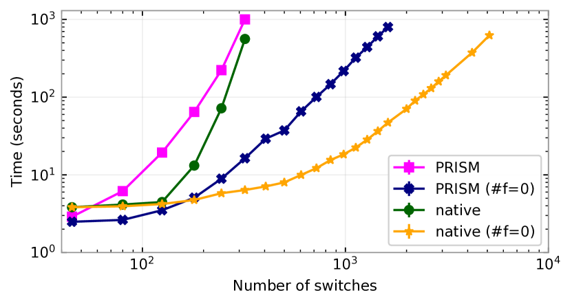
Figure 7. Scalability on a family of data center topologies.

We first measured the scalability of McNetKAT by using it to compute network models for a series of FatTree topologies of increasing size. FatTrees (Al-Fares et al., 2008) (see also Figure 6) are multi-level, multi-rooted trees that are widely used as topologies in modern data centers. FatTrees can be specified in terms of a parameter $p$ corresponding to the number of ports on each switch. A $p$-ary FatTree connects $\frac{1}{4}p^{3}$ servers using $\frac{5}{4}p^{2}$ switches. To route packets, we used a form of Equal-Cost Multipath Routing (ECMP) that randomly maps traffic flows onto shortest paths. We measured the time needed to construct the stochastic matrix representation of the program on a single machine using two backends (native and PRISM) and under two failure models (no failures and independent failures with probability $1/1000$).

Figure 7 depicts the results, several of which are worth discussing. First, the native backend scales quite well: in the absence of failures ($f=0$), it scales to a network with 5000 switches in approximately 10 minutes. This result shows that McNetKAT is able to handle networks of realistic size. Second, the native backend consistently outperforms the PRISM backend. We conjecture that the native backend is able to exploit algebraic properties of the ProbNetKAT program to better parallelize the job. Third, performance degrades in the presence of failures. This is to be expected—failures lead to more complex probability distributions which are nontrivial to represent and manipulate.

Parallel speedup.

One of the contributors to McNetKAT’s good performance is its ability to parallelize the computation of stochastic matrices across multiple cores in a machine, or even across machines in a cluster. Intuitively, because a network is a large collection of mostly independent devices, it is possible to model its global behavior by first modeling the behavior of each device in isolation, and then combining the results to obtain a network-wide model. In addition to speeding up the computation, this approach can also reduce memory usage, often a bottleneck on large inputs.

To facilitate parallelization, we added an $n$-ary disjoint branching construct to ProbNetKAT:

$$\boldsymbol{\mathsf{case}}~{}~{}\texttt{sw}\kern 0.43057pt{=}\kern 0.43057pt1~{}~{}\boldsymbol{\mathsf{then}}~{}~{}p_{1}~{}~{}\boldsymbol{\mathsf{else}}$$

$$\boldsymbol{\mathsf{case}}~{}~{}\texttt{sw}\kern 0.43057pt{=}\kern 0.43057pt2~{}~{}\boldsymbol{\mathsf{then}}~{}~{}p_{2}~{}~{}\boldsymbol{\mathsf{else}}$$

$$\quad\dots$$

$$\boldsymbol{\mathsf{case}}~{}~{}\texttt{sw}\kern 0.43057pt{=}\kern 0.43057ptn~{}~{}\boldsymbol{\mathsf{then}}~{}~{}p_{n}~{}~{}\phantom{else}$$

Semantically, this construct is equivalent to a cascade of conditionals; but the native backend compiles it in parallel using a map-reduce-style strategy, using one process per core by default.

To evaluate the impact of parallelization, we compiled two representative FatTree models ($p=14$ and $p=16$) using ECMP routing on an increasing number of cores. With $m$ cores, we used one master machine together with $r=\lceil{m/16-1}\rceil$ remote machines, adding machines one by one as needed to obtain more physical cores. The results are shown in Figure 8. We see near linear speedup on a single machine, cutting execution time by more than an order of magnitude on our 16-core test machine. Beyond a single machine, the speedup depends on the complexity of the submodels for each switch—the longer it takes to generate the matrix for each switch, the higher the speedup. For example, with a $p=16$ FatTree, we obtained a 30x speedup using 40 cores across 3 machines.

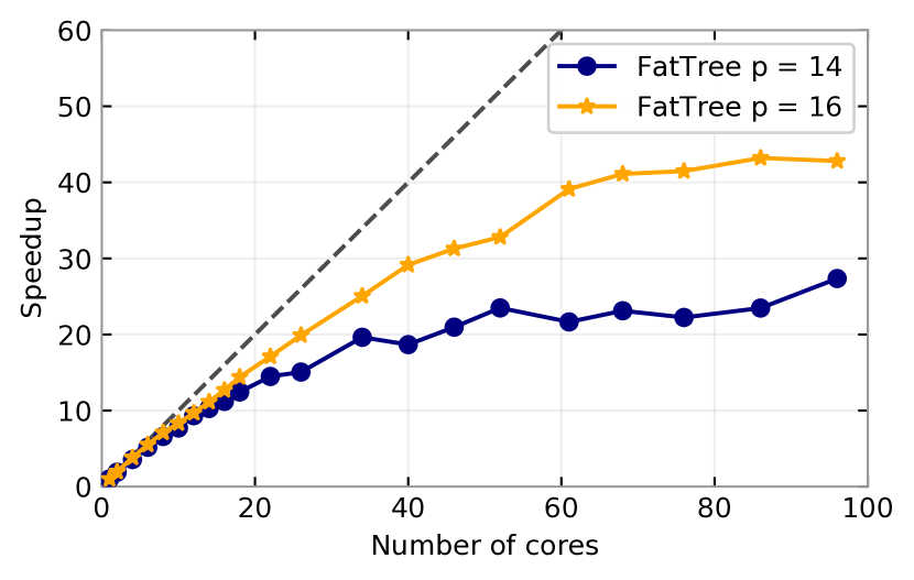
Figure 8. Speedup due to parallelization.

Comparison with other tools.

Bayonet (Gehr et al., 2018b) is a state-of-the-art tool for analyzing probabilistic networks. Whereas McNetKAT has a native backend tailored to the networking domain and a backend based on a probabilistic model checker, Bayonet programs are translated to a general-purpose probabilistic language which is then analyzed by the symbolic inference engine PSI (Gehr et al., 2016). Bayonet’s approach is more general, as it can model queues, state, and multi-packet interactions under an asynchronous scheduling model. It also supports Bayesian inference and parameter synthesis. Moreover, Bayonet is fully symbolic whereas McNetKAT uses a numerical linear algebra solver (Davis, 2004) (based on floating point arithmetic) to compute limits.

To evaluate how the performance of these approaches compares, we reproduced an experiment from the Bayonet paper that analyzes the reliability of a simple routing scheme in a family of “chain” topologies indexed by $k$, as shown in Figure 9.

Figure 9. Chain topology

For $k=1$, the network consists of four switches organized into a diamond, with a single link that fails with probability $p_{\textit{fail}}=1/1000$. For $k>1$, the network consists of $k$ diamonds linked together into a chain as shown in Figure 9. Within each diamond, switch $S_{0}$ forwards packets with equal probability to switches $S_{1}$ and $S_{2}$, which in turn forward to switch $S_{3}$. However, $S_{2}$ drops the packet if the link to $S_{3}$ fails. We analyze the probability that a packet originating at H1 is successfully delivered to H2. Our implementation does not exploit the regularity of these topologies.

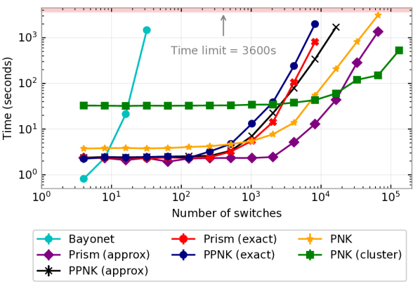
Figure 10. Scalability on chain topology.

Figure 10 gives the running time for several tools on this benchmark: Bayonet, hand-written PRISM, ProbNetKAT with the PRISM backend (PPNK), and ProbNetKAT with the native backend (PNK). Further, we ran the PRISM tools in exact and approximate mode, and we ran the ProbNetKAT backend on a single machine and on the cluster. Note that both axes in the plot are log-scaled.

We see that Bayonet scales to 32 switches in about 25 minutes, before hitting the one hour time limit and 64 GB memory limit at 48 switches. ProbNetKAT answers the same query for 2048 switches in under 10 seconds and scales to over 65000 switches in about 50 minutes on a single core, or just 2.5 minutes using a cluster of 24 machines. PRISM scales similarly to ProbNetKAT, and performs best using the hand-written model in approximate mode.

Overall, this experiment shows that for basic network verification tasks, ProbNetKAT’s domain-specific backend based on specialized data structures and an optimized linear-algebra library (Davis, 2004) can outperform an approach based on a general-purpose solver.

7. Case Study: Data Center Fault-Tolerance

$k$	$\widehat{\operatorname{M}}(\text{F10}\textsubscript{0},f_{k})$ $\equiv$ ${\mathit{teleport}}$	$\widehat{\operatorname{M}}(\text{F10}\textsubscript{3},f_{k})$ $\equiv$ ${\mathit{teleport}}$	$\widehat{\operatorname{M}}(\text{F10}\textsubscript{3,5},f_{k})$ $\equiv$ ${\mathit{teleport}}$
0	✓	✓	✓
1	✗	✓	✓
2	✗	✓	✓
3	✗	✗	✓
4	✗	✗	✗
$\infty$	✗	✗	✗

$k$	$\mathtt{compare}$ F100 F103	$\mathtt{compare}$ F103 F103,5	$\mathtt{compare}$ F103,5 $\mathit{teleport}$
0	$\equiv$	$\equiv$	$\equiv$
1	$<$	$\equiv$	$\equiv$
2	$<$	$\equiv$	$\equiv$
3	$<$	$<$	$\equiv$
4	$<$	$<$	$<$
$\infty$	$<$	$<$	$<$

Figure 11. (a) AB FatTree topology with $p=4$. (b) Evaluating $k$-resilience. (c) Comparing schemes under $k$ failures.

In this section, we go beyond benchmarks and present a case study that illustrates the utility of McNetKAT for probabilistic reasoning. Specifically, we model the F10 (Liu et al., 2013) data center design in ProbNetKAT and verify its key properties.

Data center resilience.

An influential measurement study by Gill et al. (2011) showed that data centers experience frequent failures, which have a major impact on application performance. To address this challenge, a number of data center designs have been proposed that aim to simultaneously achieve high throughput, low latency, and fault tolerance.

F10 topology.

F10 uses a novel topology called an AB FatTree, see Figure 11(a), that enhances a traditional FatTree (Al-Fares et al., 2008) with additional backup paths that can be used when failures occur. To illustrate, consider routing from $s_{7}$ to $s_{1}$ in Figure 11(a) along one of the shortest paths (in thick black). After reaching the core switch $C$ in a standard FatTree (recall Figure 6), if the aggregation switch on the downward path failed, we would need to take a 5-hop detour (shown in red) that goes down to a different edge switch, up to a different core switch, and finally down to $s_{1}$. In contrast, an AB FatTree (Liu et al., 2013) modifies the wiring of the aggregation later to provide shorter detours—e.g., a 3-hop detour (shown in blue) for the previous scenario.

F10 routing.

F10’s routing scheme uses three strategies to re-route packets after a failure occurs. If a link on the current path fails and an equal-cost path exists, the switch simply re-routes along that path. This approach is also known as equal-cost multi-path routing (ECMP). If no shortest path exist, it uses a 3-hop detour if one is available, and otherwise falls back to a 5-hop detour if necessary.

We implemented this routing scheme in ProbNetKAT in several steps. The first, F10₀, approximates the hashing behavior of ECMP by randomly selecting a port along one of the shortest paths to the destination. The second, F10₃, improves the resilience of F10₀ by augmenting it with 3-hop re-routing—e.g., consider the blue path in Figure 11(a). We find a port on $C$ that connects to a different aggregation switch $A^{\prime}$ and forward the packet to $A^{\prime}$. If there are multiple such ports which have not failed, we choose one uniformly at random. The third, F10_3,5, attempts 5-hop re-routing in cases where F10₃ is unable to find a port on $C$ whose adjacent link is up—e.g., consider the red path in Figure 11(a). The 5-hop rerouting strategy requires a flag to distinguish packets taking a detour from regular packets.

F10 network and failure model.

We model the network as discussed in Section 2, focusing on packets destined to switch 1:

$$\operatorname{M}(p)~{}\mathrel{\smash{\triangleq}}~{}in\mathop{;}\boldsymbol{\mathsf{do}}~{}(p\mathop{;}t)~{}\boldsymbol{\mathsf{while}}~{}(\neg\texttt{sw}\kern 0.43057pt{=}\kern 0.43057pt1)$$

McNetKAT automatically generates the topology program $t$ from a Graphviz description. The ingress predicate $in$ is a disjunction of switch-port tests over all ingress locations. Adding the failure model and some setup code to declare local variables tracking the health of individual links yields the complete network model:

$$\widehat{\operatorname{M}}(p,f)~{}\mathrel{\smash{\triangleq}}~{}~{} \boldsymbol{\mathsf{var}}~{}\texttt{up}_{1}\kern 0.43057pt{\shortleftarrow}\kern 0.43057pt1~{}\boldsymbol{\mathsf{in}}~{}\dots~{}\boldsymbol{\mathsf{var}}~{}\texttt{up}_{d}\kern 0.43057pt{\shortleftarrow}\kern 0.43057pt1~{}\boldsymbol{\mathsf{in}}~{}\operatorname{M}(f\mathop{;}p)$$

Here, $d$ is the maximum degree of a topology node. The entire model measures about 750 lines of ProbNetKAT code.

To evaluate the effect of different kinds of failures, we define a family of failure models $f_{k}$ indexed by the maximum number of failures $k\in\mathbb{N}\cup\{\infty\}$ that may occur, where links fail otherwise independently with probability $\mathit{pr}$; we leave $\mathit{pr}$ implicit. To simplify the analysis, we focus on failures occurring on downward paths (note that F10₀ is able to route around failures on the upward path, unless the topology becomes disconnected).

Verifying refinement.

Having implemented F10 as a series of three refinements, we would expect the probability of packet delivery to increase in each refinement, but not to achieve perfect delivery in an unbounded failure model $f_{\infty}$. Formally, we should have

$$\mathsf{drop}<\widehat{\operatorname{M}}(\text{F10}\textsubscript{0},f_{\infty}) <\widehat{\operatorname{M}}(\text{F10}\textsubscript{3},f_{\infty})$$

$$<\widehat{\operatorname{M}}(\text{F10}\textsubscript{3,5},f_{\infty})<{\mathit{teleport}}$$

where $\mathit{teleport}$ moves the packet directly to its destination, and $p<q$ means the probability assigned to every input-output pair by $q$ is greater than the probability assigned by $p$. We confirmed that these inequalities hold using McNetKAT.

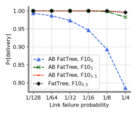
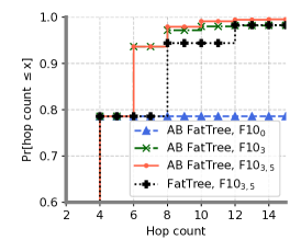
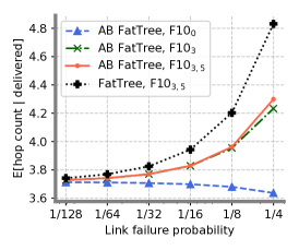
[-2em]                                (a)   (b) (c)                       

Figure 12. Case study results ($k=\infty$): (a) Probability of delivery vs. link-failure probability; (b) Increased path length due to resilience ($pr=1/4$); (c) Expected hop-count conditioned on delivery.

Verifying k-resilience.

Resilience is the key property satisfied by F10. By using McNetKAT, we were able to automatically verify that F10 is resilient to up to three failures in the AB FatTree Figure 11(a). To establish this property, we increased the parameter $k$ in our failure model $f_{k}$ while checking equivalence with teleportation (i.e., perfect delivery), as shown in Figure 11(b). The simplest scheme F10₀ drops packets when a failure occurs on the downward path, so it is 0-resilient. The F10₃ scheme routes around failures when a suitable aggregation switch is available, hence it is 2-resilient. Finally, the F10_3,5 scheme routes around failures as long as any aggregation switch is reachable, hence it is 3-resilient. If the schemes are not equivalent to $\mathit{teleport}$, we can still compare the relative resilience of the schemes using the refinement order, as shown in Figure 11(c). Our implementation also enables precise, quantitative comparisons. For example, Figure 12(a) considers a failure model in which an unbounded number of failures can occur. We find that F10₀’s delivery probability dips significantly as the failure probability increases, while both F10₃ and F10_3,5 continue to ensure high delivery probability by routing around failures.

Analyzing path stretch.

Routing schemes based on detours achieve a higher degree of resilience at the cost of increasing the lengths of forwarding paths. We can quantify this increase by augmenting our model with a counter that is incremented at each hop and analyzing the expected path length. Figure 12(b) shows the cumulative distribution function of latency as the fraction of traffic delivered within a given hop count. On AB FatTree, F10₀ delivers $\approx$80% of the traffic in 4 hops, since the maximum length of a shortest path from any edge switch to $s1$ is 4 and F10₀ does not attempt to recover from failures. F10₃ and F10_3,5 deliver the same amount of traffic when limited to at most 4 hops, but they can deliver significantly more traffic using $2$ additional hops by using 3-hop and 5-hop paths to route around failures. F10₃ also delivers more traffic with 8 hops—these are the cases when F10₃ performs 3-hop re-routing twice for a single packet as it encountered failure twice. We can also show that on a standard FatTree, F10_3,5 failures have a higher impact on latency. Intuitively, the topology does not support 3-hop re-routing. This finding supports a key claim of F10: the topology and routing scheme should be co-designed to avoid excessive path stretch. Finally, Figure 12(c) shows the expected path length conditioned on delivery. As the failure probability increases, the probability of delivery for packets routed via the core layer decreases for F10₀. Thus, the distribution of delivered packets shifts towards 2-hop paths via an aggregation switch, so the expected hop-count decreases.

8. Related Work

The most closely related system to McNetKAT is Bayonet (Gehr et al., 2018b). In contrast to the domain-specific approach followed in this paper, Bayonet uses a general-purpose probabilistic programming language and inference tool (Gehr et al., 2016). Such an approach, which reuses existing techniques, is naturally appealing. In addition, Bayonet is more expressive than McNetKAT: it supports asynchronous scheduling, stateful transformations, and probabilistic inference, making it possible to model richer phenomena, such as congestion due to packet-level interactions in queues. Of course, the extra generality does not come for free. Bayonet requires programmers to supply an upper bound on loops as the implementation is not guaranteed to find a fixed point. As discussed in Section 5, McNetKAT scales better than Bayonet on simple benchmarks. Another issue is that writing a realistic scheduler appears challenging, and one might also need to model host-level congestion control protocols to obtain accurate results. Currently Bayonet programs use deterministic or uniform schedulers and model only a few packets at a time (Gehr et al., 2018a).

Prior work on ProbNetKAT (Smolka et al., 2017) gave a measure-theoretic semantics and an implementation that approximated programs using sequences of monotonically improving estimates. While these estimates were proven to converge in the limit, (Smolka et al., 2017) offered no guarantees about the convergence rate. In fact, there are examples where the approximations do not converge after any finite number of steps, which is obviously undesirable in a tool. The implementation only scaled to 10s of switches. In contrast, this paper presents a straightforward and implementable semantics; the implementation computes limits precisely in closed form, and it scales to real-world networks with thousands of switches. McNetKAT achieves this by restricting to the guarded and history-free fragment of ProbNetKAT, sacrificing the ability to reason about multicast and path-properties directly. In practice this sacrifice seems well worth the payoff: multicast is somewhat uncommon, and we can often reason about path-properties by maintaining extra state in the packets. In particular, McNetKAT can still model the examples studied in previous work by Smolka et al. (2017).

Our work is the latest in a long line of techniques using Markov chains as a tool for representing and analyzing probabilistic programs. For an early example, see the seminal paper of Sharir et al. (1984). Markov chains are also used in many probabilistic model checkers, such as PRISM (Kwiatkowska et al., 2011a).

Beyond networking applications, there are connections to other work on verification of probabilistic programs. Di Pierro, Hankin, and Wiklicky used probabilistic abstract interpretation to statically analyze probabilistic $\lambda$-calculus (Di Pierro et al., 2005); their work was extended to a language $pWhile$, using a store and program location state space similar to Sharir et al. (1984). However, they do not deal with infinite limiting behavior beyond stepwise iteration, and do not guarantee convergence. Olejnik, Wicklicky, and Cheraghchi provided a probabilistic compiler $pwc$ for a variation of $pWhile$ (Olejnik et al., 2016); their optimizations could potentially be useful for McNetKAT. A recent survey by Gordon et al. (2014) shows how to give semantics for probabilistic processes using stationary distributions of Markov chains, and studies convergence. Similar to our approach, they use absorbing strongly connected components to represent termination. Finally, probabilistic abstract interpretation is also an active area of research (Wang et al., 2018); it would be interesting to explore applications to ProbNetKAT.

9. Conclusion

This paper presents a scalable tool for verifying probabilistic networks based on a new semantics for the history-free fragment of ProbNetKAT in terms of Markov chains. Natural directions for future work include further optimization of our implementation—e.g., using Bayesian networks to represent joint distributions compactly. We are also interested in applying McNetKAT to other systems that implement algorithms for randomized routing (Kumar et al., 2018; Singh et al., 2018), load balancing (Dixit et al., 2013), traffic monitoring (Sekar et al., 2008), anonymity (Dingledine et al., 2004), and network neutrality (Zhang et al., 2014), among others.

Appendix A ProbNetKAT Denotational Semantics

Semantics $\llbracket p\rrbracket\in\smash{2^{\mathsf{Pk}}}\to\operatorname{\mathcal{D}}(\smash{2^{\mathsf{Pk}}})$

(Discrete) Probability Monad $\operatorname{\mathcal{D}}$

$\begin{array}[]{r@{~~}c@{~~}l}\llbracket\mathsf{drop}\rrbracket(a)~{}~{}&\mathrel{\smash{\triangleq}}\hfil~{}~{}&\delta({\varnothing})\\ \llbracket\mathsf{skip}\rrbracket(a)~{}~{}&\mathrel{\smash{\triangleq}}\hfil~{}~{}&\delta({a})\\ \llbracket\mathit{f}\kern 0.43057pt{=}\kern 0.43057ptn\rrbracket(a)~{}~{}&\mathrel{\smash{\triangleq}}\hfil~{}~{}&\delta({\{\pi\in a\mid\pi.f=n\}})\\ \llbracket\mathit{f}\kern 0.43057pt{\shortleftarrow}\kern 0.43057ptn\rrbracket(a)~{}~{}&\mathrel{\smash{\triangleq}}\hfil~{}~{}&\delta({\{\pi[\mathit{f}{:=}n]\mid\pi\in a\}})\\ \llbracket\neg t\rrbracket(a)~{}~{}&\mathrel{\smash{\triangleq}}\hfil~{}~{}&\operatorname{\mathcal{D}}(\lambda b.a-b)(\llbracket t\rrbracket(a))\\ \llbracket p\mathbin{\scalebox{1.0}[1.15]{\&}}q\rrbracket(a)~{}~{}&\mathrel{\smash{\triangleq}}\hfil~{}~{}&\operatorname{\mathcal{D}}(\cup)(\llbracket p\rrbracket(a)\times\llbracket q\rrbracket(a))\\ \llbracket p\mathop{;}q\rrbracket(a)~{}~{}&\mathrel{\smash{\triangleq}}\hfil~{}~{}&\llbracket q\rrbracket^{\dagger}(\llbracket p\rrbracket(a))\\ \llbracket p\mathop{\mathrel{\oplus_{r}}}q\rrbracket(a)~{}~{}&\mathrel{\smash{\triangleq}}\hfil~{}~{}&r\cdot\llbracket p\rrbracket(a)+(1-r)\cdot\llbracket q\rrbracket(a)\\ \llbracket p^{*}\rrbracket(a)~{}~{}&\mathrel{\smash{\triangleq}}\hfil~{}~{}&\displaystyle\bigsqcup_{n\in\mathbb{N}}\llbracket p^{(n)}\rrbracket(a)\\ \lx@intercol\text{where }~{}p^{(0)}\mathrel{\smash{\triangleq}}\mathsf{skip},\hskip 6.45831ptp^{(n+1)}\mathrel{\smash{\triangleq}}\mathsf{skip}\mathbin{\scalebox{1.0}[1.15]{\&}}p\mathop{;}p^{(n)}\hfil\lx@intercol\end{array}$

$\begin{array}[]{@{}r@{\quad}l@{}}\text{Unit}&\delta:X\to\operatorname{\mathcal{D}}(X)\quad\delta(x)\mathrel{\smash{\triangleq}}\delta_{x}\\ \text{Bind}&-^{\dagger}:(X\to\operatorname{\mathcal{D}}(Y))\to\operatorname{\mathcal{D}}(X)\to\operatorname{\mathcal{D}}(Y)\\ &f^{\dagger}(\mu)(A)\mathrel{\smash{\triangleq}}\sum_{x\in X}f(x)(A)\cdot\mu(x)\end{array}$

Figure 13. ProbNetKAT semantics.

In the original ProbNetKAT language, programs manipulate sets of packet histories—non-empty, finite sequences of packets modeling trajectories through the network (Smolka et al., 2017; Foster et al., 2016). The resulting state space is uncountable and modeling the semantics properly requires full-blown measure theory as some programs generate continuous distributions. In the history-free fragment, programs manipulate sets of packets and the state space is finite, which makes the semantics considerably simpler.

Proposition A.1.

Let $\llparenthesis-\rrparenthesis$ denote the semantics defined in Smolka et al. (2017). Then for all $\mathsf{dup}$-free programs $p$ and inputs $a\in\smash{2^{\mathsf{Pk}}}$, we have $\llbracket p\rrbracket(a)=\llparenthesis p\rrparenthesis(a)$, where we identify packets and histories of length one.

Throughout this paper, we can work in the discrete space $\smash{2^{\mathsf{Pk}}}$, i.e., the set of sets of packets. An outcome (denoted by lowercase variables $a,b,c,\dots$) is a set of packets and an event (denoted by uppercase variables $A,B,C,\dots$) is a set of outcomes. Given a discrete probability measure on this space, the probability of an event is the sum of the probabilities of its outcomes.

ProbNetKAT programs are interpreted as Markov kernels on the space $\smash{2^{\mathsf{Pk}}}$. A Markov kernel is a function $\smash{2^{\mathsf{Pk}}}\to\operatorname{\mathcal{D}}(\smash{2^{\mathsf{Pk}}})$ where $\operatorname{\mathcal{D}}$ is the probability (or Giry) monad (Giry, 1982; Kozen, 1981). Thus, a program $p$ maps an input set of packets $a\in\smash{2^{\mathsf{Pk}}}$ to a distribution $\llbracket p\rrbracket(a)\in\operatorname{\mathcal{D}}(\smash{2^{\mathsf{Pk}}})$ over output sets of packets. The semantics uses the following probabilistic constructions:

• For a discrete measurable space $X$, $\operatorname{\mathcal{D}}(X)$ denotes the set of probability measures over $X$; that is, the set of countably additive functions $\mu:2^{X}\to[0,1]$ with $\mu(X)=1$.

• For a measurable function $f:X\to Y$, $\operatorname{\mathcal{D}}(f):\operatorname{\mathcal{D}}(X)\to\operatorname{\mathcal{D}}(Y)$ denotes the pushforward along $f$; that is, the function that maps a measure $\mu$ on $X$ to

  $$\operatorname{\mathcal{D}}(f)(\mu)\mathrel{\smash{\triangleq}}\mu\circ f^{-1}=\lambda A\in\Sigma_{Y}.\ \mu(\{x\in X\mid f(x)\in A\})$$

  which is called the pushforward measure on $Y$.

• The unit $\delta:X\to\operatorname{\mathcal{D}}(X)$ of the monad maps a point $x\in X$ to the point mass (or Dirac measure) $\delta_{x}\in\operatorname{\mathcal{D}}(X)$. The Dirac measure is given by

  $$\delta_{x}(A)\mathrel{\smash{\triangleq}}[x\in A]$$

  That is, the Dirac measure is $1$ if $x\in A$ and $0$ otherwise.

• The bind operation of the monad,

  $$-^{\dagger}:(X\to\operatorname{\mathcal{D}}(Y))\to\operatorname{\mathcal{D}}(X)\to\operatorname{\mathcal{D}}(Y)$$

  lifts a function $f:X\to\operatorname{\mathcal{D}}(Y)$ with deterministic inputs to a function $f^{\dagger}:\operatorname{\mathcal{D}}(X)\to\operatorname{\mathcal{D}}(Y)$ that takes random inputs. Intuitively, this is achieved by averaging the output of $f$ when the inputs are randomly distributed according to $\mu$. Formally,

  $$f^{\dagger}(\mu)(A)\mathrel{\smash{\triangleq}}\sum_{x\in X}f(x)(A)\cdot\mu(x).$$

• Given two measures $\mu\in\operatorname{\mathcal{D}}(X)$ and $\nu\in\operatorname{\mathcal{D}}(Y)$, $\mu\times\nu\in\operatorname{\mathcal{D}}(X\times Y)$ denotes their product measure. This is the unique measure satisfying

  $$(\mu\times\nu)(A\times B)=\mu(A)\cdot\nu(B)$$

  Intuitively, it models distributions over pairs of independent values.

Using these primitives, we can now make our operational intuitions precise (see Figure 13 for formal definitions). A predicate $t$ maps the set of input packets $a\in\smash{2^{\mathsf{Pk}}}$ to the subset of packets $b\subseteq a$ satisfying the predicate (with probability $1$). Hence, $\mathsf{drop}$ drops all packets (i.e., it returns the empty set) while $\mathsf{skip}$ keeps all packets (i.e., it returns the input set). The test $\mathit{f}\kern 0.43057pt{=}\kern 0.43057ptn$ returns the subset of input packets whose $\mathit{f}$-field is $n$. Negation $\neg t$ filters out the packets returned by $t$.

Parallel composition $p\mathbin{\scalebox{1.0}[1.15]{\&}}q$ executes $p$ and $q$ independently on the input set, then returns the union of their results. Note that packet sets do not model nondeterminism, unlike the usual situation in Kleene algebras—rather, they model collections of packets traversing possibly different portions of the network simultaneously. In particular, the union operation is not idempotent: $p\mathbin{\scalebox{1.0}[1.15]{\&}}p$ need not have the same semantics as $p$. Probabilistic choice $p\mathrel{\oplus_{r}}q$ feeds the input to both $p$ and $q$ and returns a convex combination of the output distributions according to $r$. Sequential composition $p\mathop{;}q$ can be thought of as a two-stage probabilistic process: it first executes $p$ on the input set to obtain a random intermediate result, then feeds that into $q$ to obtain the final distribution over outputs. The outcome of $q$ is averaged over the distribution of intermediate results produced by $p$.

We say that two programs are equivalent, denoted $p\equiv q$, if they denote the same Markov kernel, i.e. if $\llbracket p\rrbracket=\llbracket q\rrbracket$. As usual, we expect Kleene star $p^{*}$ to satisfy the characteristic fixed point equation $p^{*}\equiv\mathsf{skip}\mathbin{\scalebox{1.0}[1.15]{\&}}p\mathop{;}p^{*}$, which allows it to be unrolled ad infinitum. Thus we define it as the supremum of its finite unrollings $p^{(n)}$; see Figure 13. This supremum is taken in a CPO $(\operatorname{\mathcal{D}}(\smash{2^{\mathsf{Pk}}}),\sqsubseteq)$ of distributions that is described in more detail in Section A.1. The partial ordering $\sqsubseteq$ on packet set distributions gives rise to a partial ordering on programs: we write $p\leq q$ iff $\llbracket p\rrbracket(a)\sqsubseteq\llbracket q\rrbracket(a)$ for all inputs $a\in\smash{2^{\mathsf{Pk}}}$. Intuitively, $p\leq q$ iff $p$ produces any particular output packet $\pi$ with probability at most that of $q$ for any fixed input—$q$ has a larger probability of delivering more output packets.

A.1. The CPO $(\operatorname{\mathcal{D}}(\smash{2^{\mathsf{Pk}}}),\sqsubseteq)$

The space $\smash{2^{\mathsf{Pk}}}$ with the subset order forms a CPO $(\smash{2^{\mathsf{Pk}}},\subseteq)$. Following Saheb-Djahromi (1980), this CPO can be lifted to a CPO $(\operatorname{\mathcal{D}}(\smash{2^{\mathsf{Pk}}}),\sqsubseteq)$ on distributions over $\smash{2^{\mathsf{Pk}}}$. Because $\smash{2^{\mathsf{Pk}}}$ is a finite space, the resulting ordering $\sqsubseteq$ on distributions takes a particularly easy form:

$$\mu\sqsubseteq\nu\quad\iff\quad\mu(\{a\}{\uparrow})\leq\nu(\{a\}{\uparrow})\text{ for all }a\subseteq\mathsf{Pk}$$

where $\{a\}{\uparrow}\mathrel{\smash{\triangleq}}\{b\mid a\subseteq b\}$ denotes upward closure. Intuitively, $\nu$ produces more outputs then $\mu$. As was shown in Smolka et al. (2017), ProbNetKAT satisfies various monotonicity (and continuity) properties with respect to this ordering, including

$$a\subseteq a^{\prime}\ \implies\ \llbracket p\rrbracket(a)\sqsubseteq\llbracket p\rrbracket(a^{\prime})\qquad\text{and}\qquad n\leq m\ \implies\ \llbracket p^{(n)}\rrbracket(a)\sqsubseteq\llbracket p^{(m)}\rrbracket(a).$$

As a result, the semantics of $p^{*}$ as the supremum of its finite unrollings $p^{(n)}$ is well-defined.

While the semantics of full ProbNetKAT requires more domain theory to give a satisfactory characterization of Kleene star, a simpler characterization suffices for the history-free fragment.

Lemma A.2 (Pointwise Convergence).

Let $A\subseteq\smash{2^{\mathsf{Pk}}}$. Then for all programs $p$ and inputs $a\in\smash{2^{\mathsf{Pk}}}$,

$$\llbracket p^{*}\rrbracket(a)(A)=\lim_{n\to\infty}\llbracket p^{(n)}\rrbracket(a)(A).$$

Appendix B Omitted Proofs

Lemma B.1.

Let $A$ be a finite boolean combination of basic open sets, i.e. sets of the form $B_{a}=\{a\}\uparrow$ for $a\in\raisebox{1.0pt}{$\wp$\kern-0.7pt}_{\omega}(\mathsf{H})$, and let $\llparenthesis-\rrparenthesis$ denote the semantics from Smolka et al. (2017). Then for all programs $p$ and inputs $a\in\smash{2^{\mathsf{H}}}$,

$$\llparenthesis p^{*}\rrparenthesis(a)(A)=\lim_{n\to\infty}\llparenthesis p^{(n)}\rrparenthesis(a)(A)$$

Proof 2.

Using topological arguments, the claim follows directly from previous results: $A$ is a Cantor-clopen set by Smolka et al. (2017) (i.e., both $A$ and $\overline{A}$ are Cantor-open), so its indicator function $\mathbf{1}_{A}$ is Cantor-continuous. But $\mu_{n}\mathrel{\smash{\triangleq}}\llparenthesis p^{(n)}\rrparenthesis(a)$ converges weakly to $\mu\mathrel{\smash{\triangleq}}\llparenthesis p^{*}\rrparenthesis(a)$ in the Cantor topology (Foster et al., 2016, Theorem 4), so

$$\lim_{n\to\infty}\llparenthesis p^{(n)}\rrparenthesis(a)(A)=\lim_{n\to\infty}\int\mathbf{1}_{A}d\mu_{n}=\int\mathbf{1}_{A}d\mu=\llparenthesis p^{*}\rrparenthesis(a)(A)$$

(To see why $A$ and $\overline{A}$ are open in the Cantor topology, note that they can be written in disjunctive normal form over atoms $B_{\{h\}}$.)

Predicates in ProbNetKAT form a Boolean algebra.

Lemma B.2.

Every predicate $t$ satisfies $\llbracket t\rrbracket(a)=\delta_{a\cap b_{t}}$ for a certain packet set $b_{t}\subseteq\mathsf{Pk}$, where

• $b_{\mathsf{drop}}=\varnothing$,

• $b_{\mathsf{skip}}=\mathsf{Pk}$,

• $b_{\mathit{f}\kern 0.3014pt{=}\kern 0.3014ptn}=\{\pi\in\mathsf{Pk}\mid\pi.f=n\}$,

• $b_{\neg t}=\mathsf{Pk}-b_{t}$,

• $b_{t{\scalebox{0.66}{$\mathbin{\scalebox{1.0}[1.15]{\&}}$}}u}=b_{t}\cup b_{u}$, and

• $b_{t\mathop{;}u}=b_{t}\cap b_{u}$.

Proof 3.

For $\mathsf{drop}$, $\mathsf{skip}$, and $\mathit{f}\kern 0.43057pt{=}\kern 0.43057ptn$, the claim holds trivially. For $\neg t$, $t\mathbin{\scalebox{1.0}[1.15]{\&}}u$, and $t\mathop{;}u$, the claim follows inductively, using that $\operatorname{\mathcal{D}}(f)(\delta_{b})=\delta_{f(b)}$, $\delta_{b}\times\delta_{c}=\delta_{(b,c)}$, and that $f^{\dagger}(\delta_{b})=f(b)$. The first and last equations hold because $\langle\operatorname{\mathcal{D}},\delta,-^{\dagger}\rangle$ is a monad.

Proof of Proposition A.1.

We only need to show that for $\mathsf{dup}$-free programs $p$ and history-free inputs $a\in\smash{2^{\mathsf{Pk}}}$, $\llparenthesis p\rrparenthesis(a)$ is a distribution on packets (where we identify packets and singleton histories). We proceed by structural induction on $p$. All cases are straightforward except perhaps the case of $p^{*}$. For this case, by the induction hypothesis, all $\llbracket p^{(n)}\rrbracket(a)$ are discrete probability distributions on packet sets, therefore vanish outside $\smash{2^{\mathsf{Pk}}}$. By Lemma B.1, this is also true of the limit $\llbracket p^{*}\rrbracket(a)$, as its value on $\smash{2^{\mathsf{Pk}}}$ must be 1, therefore it is also a discrete distribution on packet sets. ∎

Proof of Lemma A.2.

This follows directly from Lemma B.1 and Proposition A.1 by noticing that any set $A\subseteq\smash{2^{\mathsf{Pk}}}$ is a finite boolean combination of basic open sets. ∎

Proof of Theorem 3.1.

It suffices to show the equality $\mathcal{B}\llbracket p\rrbracket_{ab}=\llbracket p\rrbracket(a)(\{b\})$; the remaining claims then follow by well-definedness of $\llbracket-\rrbracket$. The equality is shown using Lemma A.2 and a routine induction on $p$:

For $p=\mathsf{drop},\mathsf{skip},f\kern 0.43057pt{=}\kern 0.43057ptn,f\kern 0.43057pt{\shortleftarrow}\kern 0.43057ptn$ we have

$$\llbracket p\rrbracket(a)(\{b\})=\delta_{c}(\{b\})=[b=c]=\mathcal{B}\llbracket p\rrbracket_{ab}$$

for $c=\varnothing,a,\{\pi\in a\mid\pi.f=n\},\{\pi[f:=n]\mid\pi\in a\}$, respectively.

For $\neg t$ we have,

$$\begin{array}[]{rl@{\quad}l@{\quad}l}\mathcal{B}\llbracket\neg t\rrbracket_{ab}&=[b\subseteq a]\cdot\mathcal{B}\llbracket t\rrbracket_{a,a-b}\\ &=[b\subseteq a]\cdot\llbracket t\rrbracket(a)(\{a-b\})&&\text{(IH)}\\ &=[b\subseteq a]\cdot[a-b=a\cap b_{t}]&&\text{(\lx@cref{creftype~refnum}{lem:preds-boolean-algebra})}\\ &=[b\subseteq a]\cdot[a-b=a-(\mathsf{H}-b_{t})]\\ &=[b=a\cap(H-b_{t})]\\ &=\llbracket\neg t\rrbracket(a)(b)&&\text{(\lx@cref{creftype~refnum}{lem:preds-boolean-algebra})}\end{array}$$

For $p\mathbin{\scalebox{1.0}[1.15]{\&}}q$, letting $\mu=\llbracket p\rrbracket(a)$ and $\nu=\llbracket q\rrbracket(a)$ we have

$$\begin{array}[]{rl@{\quad}l@{\quad}l}\llbracket p\mathbin{\scalebox{1.0}[1.15]{\&}}q\rrbracket(a)(\{b\})&=(\mu\times\nu)(\{(b_{1},b_{2})\mid b_{1}\cup b_{2}=b\})\\ &=\sum_{b_{1},b_{2}}[b_{1}\cup b_{2}=b]\cdot(\mu\times\nu)(\{(b_{1},b_{2})\})&&\\ &=\sum_{b_{1},b_{2}}[b_{1}\cup b_{2}=b]\cdot\mu(\{b_{1}\})\cdot\nu(\{b_{2}\})\\ &=\sum_{b_{1},b_{2}}[b_{1}\cup b_{2}=b]\cdot\mathcal{B}\llbracket p\rrbracket_{ab_{1}}\cdot\mathcal{B}\llbracket q\rrbracket_{ab_{2}}&&\text{(IH)}\\ &=\mathcal{B}\llbracket p\mathbin{\scalebox{1.0}[1.15]{\&}}q\rrbracket_{ab}\end{array}$$

where we use in the second step that $b\subseteq\mathsf{Pk}$ is finite, thus $\{(b_{1},b_{2})\mid b_{1}\cup b_{2}=b\}$ is finite.

For $p\mathop{;}q$, let $\mu=\llbracket p\rrbracket(a)$ and $\nu_{c}=\llbracket q\rrbracket(c)$ and recall that $\mu$ is a discrete distribution on $\smash{2^{\mathsf{Pk}}}$. Thus

$$\begin{array}[]{rl@{\quad}l@{\quad}l}\llbracket p\mathop{;}q\rrbracket(a)(\{b\})&=\sum_{c\in\smash{2^{\mathsf{Pk}}}}\nu_{c}(\{b\})\cdot\mu(\{c\})\\ &=\sum_{c\in\smash{2^{\mathsf{Pk}}}}\mathcal{B}\llbracket q\rrbracket_{c,b}\cdot\mathcal{B}\llbracket p\rrbracket_{a,c}\\ &=\mathcal{B}\llbracket p\mathop{;}q\rrbracket_{ab}.\end{array}$$

For $p\oplus_{r}q$, the claim follows directly from the induction hypotheses.

Finally, for $p^{*}$, we know that $\mathcal{B}\llbracket p^{(n)}\rrbracket_{ab}=\llbracket p^{(n)}\rrbracket(a)(\{b\})$ by induction hypothesis. The key to proving the claim is Lemma A.2, which allows us to take the limit on both sides and deduce

$$\mathcal{B}\llbracket p^{*}\rrbracket_{ab}=\lim_{n\to\infty}\mathcal{B}\llbracket p^{(n)}\rrbracket_{ab}=\lim_{n\to\infty}\llbracket p^{(n)}\rrbracket(a)(\{b\})=\llbracket p^{*}\rrbracket(a)(\{b\}).\qed$$

Proof of Lemma 4.1.

For arbitrary $a,b\subseteq\mathsf{Pk}$, we have

$$\sum_{a^{\prime},b^{\prime}}\mathcal{S}\llbracket p\rrbracket_{(a,b),(a^{\prime},b^{\prime})} =\sum_{a^{\prime},b^{\prime}}[b^{\prime}=a\cup b]\cdot\mathcal{B}\llbracket p\rrbracket_{a,a^{\prime}}$$

$$=\sum_{a^{\prime}}\Big{(}\sum_{b^{\prime}}[b^{\prime}=a\cup b]\Big{)}\cdot\mathcal{B}\llbracket p\rrbracket_{a,a^{\prime}}$$

$$=\sum_{a^{\prime}}\mathcal{B}\llbracket p\rrbracket_{a,a^{\prime}}=1$$

where in the last step, we use that $\mathcal{B}\llbracket p\rrbracket$ is stochastic (Theorem 3.1). ∎

Proof of Lemma 4.3.

By induction on $n\geq 0$. For $n=0$, we have

$$\sum_{a^{\prime}}[b^{\prime}=a^{\prime}\cup b]\cdot\mathcal{B}\llbracket p^{(n)}\rrbracket_{a,a^{\prime}} =\sum_{a^{\prime}}[b^{\prime}=a^{\prime}\cup b]\cdot\mathcal{B}\llbracket\mathsf{skip}\rrbracket_{a,a^{\prime}}$$

$$=\sum_{a^{\prime}}[b^{\prime}=a^{\prime}\cup b]\cdot[a=a^{\prime}]$$

$$=[b^{\prime}=a\cup b]$$

$$=[b^{\prime}=a\cup b]\cdot\sum_{a^{\prime}}\mathcal{B}\llbracket p\rrbracket_{a,a^{\prime}}$$

$$=\sum_{a^{\prime}}\mathcal{S}\llbracket p\rrbracket_{(a,b),(a^{\prime},b^{\prime})}$$

In the induction step ($n>0$),

$$\phantom{={}}\sum_{a^{\prime}}[b^{\prime}=a^{\prime}\cup b]\cdot\mathcal{B}\llbracket p^{(n)}\rrbracket_{a,a^{\prime}}$$

$$=\sum_{a^{\prime}}[b^{\prime}=a^{\prime}\cup b]\cdot\mathcal{B}\llbracket\mathsf{skip}\mathbin{\scalebox{1.0}[1.15]{\&}}p\mathop{;}p^{(n-1)}\rrbracket_{a,a^{\prime}}$$

$$=\sum_{a^{\prime}}[b^{\prime}=a^{\prime}\cup b]\cdot\sum_{c}[a^{\prime}=a\cup c]\cdot\mathcal{B}\llbracket p\mathop{;}p^{(n-1)}\rrbracket_{a,c}$$

$$=\sum_{c}\left(\sum_{a^{\prime}}[b^{\prime}=a^{\prime}\cup b]\cdot[a^{\prime}=a\cup c]\right)\cdot\sum_{k}\mathcal{B}\llbracket p\rrbracket_{a,k}\cdot\mathcal{B}\llbracket p^{(n-1)}\rrbracket_{k,c}$$

$$=\sum_{c,k}[b^{\prime}=a\cup c\cup b]\cdot\mathcal{B}\llbracket p\rrbracket_{a,k}\cdot\mathcal{B}\llbracket p^{(n-1)}\rrbracket_{k,c}$$

$$=\sum_{k}\mathcal{B}\llbracket p\rrbracket_{a,k}\cdot\sum_{a^{\prime}}[b^{\prime}=a^{\prime}\cup(a\cup b)]\cdot\mathcal{B}\llbracket p^{(n-1)}\rrbracket_{k,a^{\prime}}$$

$$=\sum_{k}\mathcal{B}\llbracket p\rrbracket_{a,k}\cdot\sum_{a^{\prime}}\mathcal{S}\llbracket p\rrbracket^{n}_{(k,a\cup b),(a^{\prime},b^{\prime})}$$

$$=\sum_{a^{\prime}}\sum_{k_{1},k_{2}}[k_{2}=a\cup b]\cdot\mathcal{B}\llbracket p\rrbracket_{a,k_{1}}\cdot\mathcal{S}\llbracket p\rrbracket^{n}_{(k_{1},k_{2}),(a^{\prime},b^{\prime})}$$

$$=\sum_{a^{\prime}}\sum_{k_{1},k_{2}}\mathcal{S}\llbracket p\rrbracket_{(a,b)(k_{1},k_{2})}\cdot\mathcal{S}\llbracket p\rrbracket^{n}_{(k_{1},k_{2}),(a^{\prime},b^{\prime})}$$

$$=\sum_{a^{\prime}}\mathcal{S}\llbracket p\rrbracket^{n+1}_{(a,b),(a^{\prime},b^{\prime})}\qed$$

Lemma B.3.

The matrix $X=I-Q$ in Equation (3) of Section 4 is invertible.

Proof 4.

Let $S$ be a finite set of states, $|S|=n$, $M$ an $S\times S$ substochastic matrix ($M_{st}\geq 0$, $M\mathbf{1}\leq\mathbf{1}$). A state $s$ is defective if $(M\mathbf{1})_{s}<1$. We say $M$ is stochastic if $M\mathbf{1}=\mathbf{1}$, irreducible if $(\sum_{i=0}^{n-1}M^{i})_{st}>0$ (that is, the support graph of $M$ is strongly connected), and aperiodic if all entries of some power of $M$ are strictly positive.

We show that if $M$ is substochastic such that every state can reach a defective state via a path in the support graph, then the spectral radius of $M$ is strictly less than $1$. Intuitively, all weight in the system eventually drains out at the defective states.

Let $e_{s}$, $s\in S$, be the standard basis vectors. As a distribution, $e_{s}^{T}$ is the unit point mass on $s$. For $A\subseteq S$, let $e_{A}=\sum_{s\in A}e_{s}$. The $L_{1}$-norm of a substochastic vector is its total weight as a distribution. Multiplying on the right by $M$ never increases total weight, but will strictly decrease it if there is nonzero weight on a defective state. Since every state can reach a defective state, this must happen after $n$ steps, thus $\|e_{s}^{T}M^{n}\|_{1}<1$. Let $c=\max_{s}\|e_{s}^{T}M^{n}\|_{1}<1$. For any $y=\sum_{s}a_{s}e_{s}$,

$$\|y^{T}M^{n}\|_{1} =\|(\sum_{s}a_{s}e_{s})^{T}M^{n}\|_{1}$$

$$\leq\sum_{s}|a_{s}|\cdot\|e_{s}^{T}M^{n}\|_{1}\leq\sum_{s}|a_{s}|\cdot c=c\cdot\|y^{T}\|_{1}.$$

Then $M^{n}$ is contractive in the $L_{1}$ norm, so $|\lambda|<1$ for all eigenvalues $\lambda$. Thus $I-M$ is invertible because $1$ is not an eigenvalue of $M$.

Proof of Proposition 4.6.

1. It suffices to show that $USU=SU$. Suppose that

   $$\operatorname*{\mathbf{Pr}}[(a,b)\xrightarrow{USU}_{1}(a^{\prime},b^{\prime})]=p>0.$$

   It suffices to show that this implies

   $$\operatorname*{\mathbf{Pr}}[(a,b)\xrightarrow{SU}_{1}(a^{\prime},b^{\prime})]=p.$$

   If $(a,b)$ is saturated, then we must have $(a^{\prime},b^{\prime})=(\varnothing,b)$ and

   $$\operatorname*{\mathbf{Pr}}[(a,b)\xrightarrow{USU}_{1}(\varnothing,b)]=1=\operatorname*{\mathbf{Pr}}[(a,b)\xrightarrow{SU}_{1}(\varnothing,b)]$$

   If $(a,b)$ is not saturated, then $(a,b)\xrightarrow{U}_{1}(a,b)$ with probability $1$ and therefore

   $$\operatorname*{\mathbf{Pr}}[(a,b)\xrightarrow{USU}_{1}(a^{\prime},b^{\prime})]=\operatorname*{\mathbf{Pr}}[(a,b)\xrightarrow{SU}_{1}(a^{\prime},b^{\prime})]$$

2. Since $S$ and $U$ are stochastic, clearly $SU$ is a MC. Since $SU$ is finite state, any state can reach an absorbing communication class. (To see this, note that the reachability relation $\xrightarrow{SU}$ induces a partial order on the communication classes of $SU$. Its maximal elements are necessarily absorbing, and they must exist because the state space is finite.) It thus suffices to show that a state set $C\subseteq\smash{2^{\mathsf{Pk}}}\times\smash{2^{\mathsf{Pk}}}$ in $SU$ is an absorbing communication class iff $C=\{(\varnothing,b)\}$ for some $b\subseteq\mathsf{Pk}$.

   1. Observe that $\varnothing\xrightarrow{B}_{1}a^{\prime}$ iff $a^{\prime}=\varnothing$. Thus $(\varnothing,b)\xrightarrow{S}_{1}(a^{\prime},b^{\prime})$ iff $a^{\prime}=\varnothing$ and $b^{\prime}=b$, and likewise $(\varnothing,b)\xrightarrow{U}_{1}(a^{\prime},b^{\prime})$ iff $a^{\prime}=\varnothing$ and $b^{\prime}=b$. Thus $(\varnothing,b)$ is an absorbing state in $SU$ as required.

   2. First observe that by monotonicity of $SU$ (Lemma 4.5), we have $b=b^{\prime}$ whenever $(a,b)\xleftrightarrow{SU}(a^{\prime},b^{\prime})$; thus there exists a fixed $b_{C}$ such that $(a,b)\in C$ implies $b=b_{C}$.

      Now pick an arbitrary state $(a,b_{C})\in C$. It suffices to show that $(a,b_{C})\xrightarrow{SU}(\varnothing,b_{C})$, because that implies $(a,b_{C})\xleftrightarrow{SU}(\varnothing,b_{C})$, which in turn implies $a=\varnothing$. But the choice of $(a,b_{C})\in C$ was arbitrary, so that would mean $C=\{(\varnothing,b_{C})\}$ as claimed.

      To show that $(a,b_{C})\xrightarrow{SU}(\varnothing,b_{C})$, pick arbitrary states such that

      $$(a,b_{C})\xrightarrow{S}(a^{\prime},b^{\prime})\xrightarrow{U}_{1}(a^{\prime\prime},b^{\prime\prime})$$

      and recall that this implies $(a,b_{C})\xrightarrow{SU}(a^{\prime\prime},b^{\prime\prime})$ by claim (1). Then $(a^{\prime\prime},b^{\prime\prime})\xrightarrow{SU}(a,b_{C})$ because $C$ is absorbing, and thus $b_{C}=b^{\prime}=b^{\prime\prime}$ by monotonicity of $S$, $U$, and $SU$. But $(a^{\prime},b^{\prime})$ was chosen as an arbitrary state $S$-reachable from $(a,b_{C})$, so $(a,b)$ and by transitivity $(a^{\prime},b^{\prime})$ must be saturated. Thus $a^{\prime\prime}=\varnothing$ by the definition of $U$. ∎

Proof of Theorem 4.7.

Using Proposition 4.6.1 in the second step and equation 4 in the last step,

$$\lim_{n\to\infty}\sum_{a^{\prime}}S^{n}_{(a,b),(a^{\prime},b^{\prime})} =\lim_{n\to\infty}\sum_{a^{\prime}}(S^{n}U)_{(a,b),(a^{\prime},b^{\prime})}$$

$$=\lim_{n\to\infty}\sum_{a^{\prime}}(SU)^{n}_{(a,b),(a^{\prime},b^{\prime})}$$

$$=\sum_{a^{\prime}}(SU)^{\infty}_{(a,b),(a^{\prime},b^{\prime})}=(SU)^{\infty}_{(a,b),(\varnothing,b^{\prime})}$$

$(SU)^{\infty}$ is computable because $S$ and $U$ are matrices over $\mathbb{Q}$ and hence so is $(I-Q)^{-1}R$. ∎

Corollary B.4.

For programs $p$ and $q$, it is decidable whether $p\equiv q$.

Proof of Corollary B.4.

Recall from Corollary 3.2 that it suffices to compute the finite rational matrices $\mathcal{B}\llbracket p\rrbracket$ and $\mathcal{B}\llbracket q\rrbracket$ and check them for equality. But Theorem 4.7 together with Proposition 4.2 gives us an effective mechanism to compute $\mathcal{B}\llbracket-\rrbracket$ in the case of Kleene star, and $\mathcal{B}\llbracket-\rrbracket$ is straightforward to compute in all other cases. Summarizing the full chain of equalities, we have:

$$\llbracket p^{*}\rrbracket(a)(\{b\})=\mathcal{B}\llbracket p^{*}\rrbracket_{a,b}=\lim_{n\to\infty}\mathcal{B}\llbracket p^{(n)}\rrbracket_{a,b}=\lim_{n\to\infty}\sum_{a^{\prime}}\mathcal{S}\llbracket p\rrbracket^{n}_{(a,\varnothing),(a^{\prime},b)}=(SU)^{\infty}_{(a,\varnothing),(\varnothing,b)}$$

following from Theorem 3.1, Definition of $\mathcal{B}\llbracket-\rrbracket$, Proposition 4.2, and finally Theorem 4.7. ∎

Appendix C Handling Full ProbNetKAT: Obstacles and Challenges

History-free ProbNetKAT can describe sophisticated network routing schemes under various failure models, and the program semantics can be computed exactly. Performing quantitative reasoning in full ProbNetKAT appears significantly more challenging. We illustrate some of the difficulties in deciding program equivalence; recall that this is decidable for the history-free fragment (Corollary B.4).

The main difference in the original ProbNetKAT language is an additional primitive $\mathsf{dup}$. Intuitively, this command duplicates a packet $\pi\in\mathsf{Pk}$ and outputs the word $\pi\pi\in\mathsf{H}$, where $\mathsf{H}=\mathsf{Pk}^{*}$ is the set of non-empty, finite sequences of packets. An element of $\mathsf{H}$ is called a packet history, representing a log of previous packet states. ProbNetKAT policies may only modify the first (head) packet of each history; $\mathsf{dup}$ fixes the current head packet into the log by copying it. In this way, ProbNetKAT policies can compute distributions over the paths used to forward packets, instead of just over the final output packets.

However, with $\mathsf{dup}$, the semantics of ProbNetKAT becomes significantly more complex. Policies $p$ now transform sets of packet histories $a\in\smash{2^{\mathsf{H}}}$ to distributions $\llbracket p\rrbracket(a)\in\operatorname{\mathcal{D}}(\smash{2^{\mathsf{H}}})$. Since $\smash{2^{\mathsf{H}}}$ is uncountable, these distributions are no longer guaranteed to be discrete, and formalizing the semantics requires full-blown measure theory (see prior work for details (Smolka et al., 2017)).

Without $\mathsf{dup}$, policies operate on sets of packets $\smash{2^{\mathsf{Pk}}}$; crucially, this is a finite set and we can represent each set with a single state in a finite Markov chain. With $\mathsf{dup}$, policies operate on sets of packet histories $\smash{2^{\mathsf{H}}}$. Since this set is not finite—in fact, it is not even countable—encoding each packet history as a state would give a Markov chain with infinitely many states. Procedures for deciding equivalence are not known for such systems in general.

While in principle there could be a more compact representation of general ProbNetKAT policies as finite Markov chains or other models where equivalence is decidable, (e.g., weighted or probabilistic automata (Droste et al., 2009) or quantitative variants of regular expressions (Alur et al., 2016)), we suspect that deciding equivalence in the presence of $\mathsf{dup}$ may be intractable. As circumstantial evidence, ProbNetKAT policies can simulate a probabilistic variant of multitape automaton originally introduced by Rabin and Scott (1959). We specialize the definition here to two tapes, for simplicity, but ProbNetKAT programs can encode any multitape automata with any fixed number of tapes.

Definition C.1.

Let $A$ be a finite alphabet. A probabilistic multitape automaton is defined by a tuple $(S,s_{0},\rho,\tau)$ where $S$ is a finite set of states; $s_{0}\in S$ is the initial state; $\rho:S\to(A\cup\{\_\})^{2}$ maps each state to a pair of letters $(u,v)$, where either $u$ or $v$ may be a special blank character $\_$; and the transition function $\tau:S\to\operatorname{\mathcal{D}}(S)$ gives the probability of transitioning from one state to another.

The semantics of an automaton can be defined as a probability measure on the space $A^{\infty}\times A^{\infty}$, where $A^{\infty}$ is the set of finite and (countably) infinite words over the alphabet $A$. Roughly, these measures are fully determined by the probabilities of producing any two finite prefixes of words $(w,w^{\prime})\in A^{*}\times A^{*}$.

Presenting the formal semantics would require more concepts from measure theory and take us far afield, but the basic idea is simple to describe. An infinite trace of a probabilistic multitape automaton over states $s_{0},s_{1},s_{2},\dots$ gives a sequence of pairs of (possibly blank) letters:

$$\rho(s_{0}),\rho(s_{1}),\rho(s_{2})\dots$$

By concatenating these pairs together and dropping all blank characters, a trace induces two (finite or infinite) words over the alphabet $A$. For example, the sequence,

$$(a_{0},\_),(a_{1},\_),(\_,a_{2}),\dots$$

gives the words $a_{0}a_{1}\dots$ and $a_{2}\dots$. Since the traces are generated by the probabilistic transition function $\tau$, each automaton gives rise to a probability measure over pairs of infinite words.

Probabilistic multitape automata can be encoded as ProbNetKAT policies with $\mathsf{dup}$. We sketch the idea here, deferring further details to Appendix D. Suppose we are given an automaton $(S,s_{0},\rho,\tau)$. We build a ProbNetKAT policy over packets with two fields, $\boldsymbol{\mathsf{st}}$ and $\boldsymbol{\mathsf{id}}$. The first field $\boldsymbol{\mathsf{st}}$ ranges over the states $S$ and the alphabet $A$, while the second field $\boldsymbol{\mathsf{id}}$ is either $1$ or $2$; we suppose the input set has exactly two packets labeled with $\boldsymbol{\mathsf{id}}=1$ and $\boldsymbol{\mathsf{id}}=2$. In a set of packet history, the two active packets have the same value for $\boldsymbol{\mathsf{st}}\in S$—this represents the current state in the automaton. Past packets in the history have $\boldsymbol{\mathsf{st}}\in A$, representing the words produced so far; the first and second components of the output are tracked by the histories with $\boldsymbol{\mathsf{id}}=1$ and $\boldsymbol{\mathsf{id}}=2$. We can encode the transition function $\tau$ as a probabilistic choice in ProbNetKAT, updating the current state $\boldsymbol{\mathsf{st}}$ of all packets, and recording non-blank letters produced by $\rho$ in the two components by applying $\mathsf{dup}$ on packets with the corresponding value of $\boldsymbol{\mathsf{id}}$.

Intuitively, a set of packet histories generated by the resulting ProbNetKAT term describes a pair of words generated by the original automaton. With a bit more bookkeeping (see Appendix D), we can show that two probabilistic multitape automata are equivalent if and only if their encoded ProbNetKAT policies are equivalent. Thus, deciding equivalence for ProbNetKAT with $\mathsf{dup}$ is harder than deciding equivalence for probabilistic multitape automata; similar reductions have been considered before for showing undecidability of related problems about KAT (Kozen, 1997) and probabilistic NetKAT (Kahn, 2017).

Deciding equivalence between probabilistic multitape automata is a challenging open problem. In the special case where only one word is generated (say, when the second component produced is always blank), these automata are equivalent to standard automata with $\varepsilon$-transitions (e.g., see Mohri (2000)). In this setting, non-productive steps can be eliminated and the automata can be modeled as finite state Markov chains, where equivalence is decidable. In our setting, however, steps producing blank letters in one component may produce non-blank letters in the other. As a result, it is not clear how to eliminate these steps and encode our automata as Markov chains. Removing probabilities, it is known that equivalence between non-deterministic multitape automata is undecidable (Griffiths, 1968). Deciding equivalence of deterministic multitape automata remained a challenging open question for many years, until Harju and Karhumäki (1991) surprisingly settled the question positively; Worrell (2013) later gave an alternative proof. If equivalence of probabilistic multitape automata is undecidable, then equivalence is undecidable for ProbNetKAT programs as well. However if equivalence turns out to be decidable, the proof technique may shed light on how to decide equivalence for the full ProbNetKAT language.

Appendix D Encoding 2-Generative Automata in Full ProbNetKAT

To keep notation light, we describe our encoding in the special case where the alphabet $A=\{x,y\}$, there are four states $S=\{s_{1},s_{2},s_{3},s_{4}\}$, the initial state is $s_{1}$, and the output function $\rho$ is

$$\rho(s_{1})=(x,\_)\qquad\rho(s_{2})=(y,\_)\qquad\rho(s_{3})=(\_,x)\qquad\rho(s_{4})=(\_,y).$$

Encoding general automata is not much more complicated. Let $\tau:S\to\operatorname{\mathcal{D}}(S)$ be a given transition function; we write $p_{i,j}$ for $\tau(s_{i})(s_{j})$. We will build a ProbNetKAT policy simulating this automaton. Packets have two fields, $\boldsymbol{\mathsf{st}}$ and $\boldsymbol{\mathsf{id}}$, where $\boldsymbol{\mathsf{st}}$ ranges over $S\cup A\cup\{\bullet\}$ and $\boldsymbol{\mathsf{id}}$ ranges over $\{1,2\}$. Define:

$$p\mathrel{\smash{\triangleq}}\boldsymbol{\mathsf{st}}\kern 0.43057pt{=}\kern 0.43057pts_{1}\mathop{;}\boldsymbol{\mathsf{loop}}^{*}\mathop{;}\boldsymbol{\mathsf{st}}\kern 0.43057pt{\shortleftarrow}\kern 0.43057pt\bullet$$

The initialization keeps packets that start in the initial state, while the final command marks histories that have exited the loop by setting $\boldsymbol{\mathsf{st}}$ to be the special letter $\bullet$.

The main program $\boldsymbol{\mathsf{loop}}$ first branches on the current state $\boldsymbol{\mathsf{st}}$:

$$\boldsymbol{\mathsf{loop}}\mathrel{\smash{\triangleq}}\text{case }\begin{cases}\boldsymbol{\mathsf{st}}\kern 0.43057pt{=}\kern 0.43057pts_{1}:\boldsymbol{\mathsf{state}}1\\ \boldsymbol{\mathsf{st}}\kern 0.43057pt{=}\kern 0.43057pts_{2}:\boldsymbol{\mathsf{state}}2\\ \boldsymbol{\mathsf{st}}\kern 0.43057pt{=}\kern 0.43057pts_{3}:\boldsymbol{\mathsf{state}}3\\ \boldsymbol{\mathsf{st}}\kern 0.43057pt{=}\kern 0.43057pts_{4}:\boldsymbol{\mathsf{state}}4\end{cases}$$

Then, the policy simulates the behavior from each state. For instance:

$$\boldsymbol{\mathsf{state1}}\mathrel{\smash{\triangleq}}\bigoplus\begin{cases}(\boldsymbol{\mathsf{if}}~{}\boldsymbol{\mathsf{id}}\kern 0.43057pt{=}\kern 0.43057pt1~{}\boldsymbol{\mathsf{then}}~{}\boldsymbol{\mathsf{st}}\kern 0.43057pt{\shortleftarrow}\kern 0.43057ptx\mathop{;}\mathsf{dup}~{}\boldsymbol{\mathsf{else}}~{}\mathsf{skip})\mathop{;}\boldsymbol{\mathsf{st}}\kern 0.43057pt{\shortleftarrow}\kern 0.43057pts_{1}\mathbin{\scalebox{0.9}{\raisebox{0.6pt}{@}}}p_{1,1},\\ (\boldsymbol{\mathsf{if}}~{}\boldsymbol{\mathsf{id}}\kern 0.43057pt{=}\kern 0.43057pt1~{}\boldsymbol{\mathsf{then}}~{}\boldsymbol{\mathsf{st}}\kern 0.43057pt{\shortleftarrow}\kern 0.43057pty\mathop{;}\mathsf{dup}~{}\boldsymbol{\mathsf{else}}~{}\mathsf{skip})\mathop{;}\boldsymbol{\mathsf{st}}\kern 0.43057pt{\shortleftarrow}\kern 0.43057pts_{2}\mathbin{\scalebox{0.9}{\raisebox{0.6pt}{@}}}p_{1,2},\\ (\boldsymbol{\mathsf{if}}~{}\boldsymbol{\mathsf{id}}\kern 0.43057pt{=}\kern 0.43057pt2~{}\boldsymbol{\mathsf{then}}~{}\boldsymbol{\mathsf{st}}\kern 0.43057pt{\shortleftarrow}\kern 0.43057ptx\mathop{;}\mathsf{dup}~{}\boldsymbol{\mathsf{else}}~{}\mathsf{skip})\mathop{;}\boldsymbol{\mathsf{st}}\kern 0.43057pt{\shortleftarrow}\kern 0.43057pts_{3}\mathbin{\scalebox{0.9}{\raisebox{0.6pt}{@}}}p_{1,3},\\ (\boldsymbol{\mathsf{if}}~{}\boldsymbol{\mathsf{id}}\kern 0.43057pt{=}\kern 0.43057pt2~{}\boldsymbol{\mathsf{then}}~{}\boldsymbol{\mathsf{st}}\kern 0.43057pt{\shortleftarrow}\kern 0.43057pty\mathop{;}\mathsf{dup}~{}\boldsymbol{\mathsf{else}}~{}\mathsf{skip})\mathop{;}\boldsymbol{\mathsf{st}}\kern 0.43057pt{\shortleftarrow}\kern 0.43057pts_{4}\mathbin{\scalebox{0.9}{\raisebox{0.6pt}{@}}}p_{1,4}\end{cases}$$

The policies $\boldsymbol{\mathsf{state2}},\boldsymbol{\mathsf{state3}},\boldsymbol{\mathsf{state4}}$ are defined similarly.

Now, suppose we are given two probabilistic multitape automata $W,W^{\prime}$ that differ only in their transition functions. For simplicity, we will further assume that both systems have strictly positive probability of generating a letter in either component in finitely many steps from any state. Suppose they generate distributions $\mu,\mu^{\prime}$ respectively over pairs of infinite words $A^{\omega}\times A^{\omega}$. Now, consider the encoded ProbNetKAT policies $p,p^{\prime}$. We argue that $\llbracket p\rrbracket=\llbracket q\rrbracket$ if and only if $\mu=\mu^{\prime}$.

First, it can be shown that $\llbracket p\rrbracket=\llbracket p^{\prime}\rrbracket$ if and only if $\llbracket p\rrbracket(e)=\llbracket p^{\prime}\rrbracket(e)$, where

$$e\mathrel{\smash{\triangleq}}\{\pi\pi\mid\pi\in\mathsf{Pk}\}.$$

Let $\nu=\llbracket p\rrbracket(e)$ and $\nu^{\prime}=\llbracket p^{\prime}\rrbracket(e)$. The key connection between the automata and the encoded policies is the following equality:

(5) $$\mu(S_{u,v})=\nu(T_{u,v})$$

for every pair of finite prefixes $u,v\in A^{*}$. In the automata distribution on the left, $S_{u,v}\subseteq A^{\omega}\times A^{\omega}$ consists of all pairs of infinite strings where $u$ is a prefix of the first component and $v$ is a prefix of the second component. In the ProbNetKAT distribution on the right, we first encode $u$ and $v$ as packet histories. For $i\in\{1,2\}$ representing the component and $w\in A^{*}$ a finite word, define the history

$$\mathit{h}_{i}(w)\in\mathsf{H}\mathrel{\smash{\triangleq}}(\boldsymbol{\mathsf{st}}=\bullet,\boldsymbol{\mathsf{id}}=i),(\boldsymbol{\mathsf{st}}=w[|w|],\boldsymbol{\mathsf{id}}=i),\dots,(\boldsymbol{\mathsf{st}}=w[1],\boldsymbol{\mathsf{id}}=i),(\boldsymbol{\mathsf{st}}=s_{1},\boldsymbol{\mathsf{id}}=i).$$

The letters of the word $w$ are encoded in reverse order because by convention, the head/newest packet is written towards the left-most end of a packet history, while the oldest packet is written towards the right-most end. For instance, the final letter $w[|w|]$ is the most recent (i.e., the latest) letter produced by the policy. Then, $T_{u,v}$ is the set of all history sets including $\mathit{h}_{1}(u)$ and $\mathit{h}_{2}(v)$:

$$T_{u,v}\mathrel{\smash{\triangleq}}\{a\in\smash{2^{\mathsf{H}}}\mid\mathit{h}_{1}(u)\in a,\mathit{h}_{2}(v)\in a\}.$$

Now $\llbracket p\rrbracket=\llbracket p^{\prime}\rrbracket$ implies $\mu=\mu^{\prime}$, since 5 gives

$$\mu(S_{u,v})=\mu^{\prime}(S_{u,v}).$$

The reverse implication is a bit more delicate. Again by 5, we have

$$\nu(T_{u,v})=\nu^{\prime}(T_{u,v}).$$

We need to extend this equality to all cones, defined by packet histories $\mathit{h}$:

$$B_{\mathit{h}}\mathrel{\smash{\triangleq}}\{a\in\smash{2^{\mathsf{H}}}\mid\mathit{h}\in a\}.$$

This follows by expressing $B_{\mathit{h}}$ as boolean combinations of $T_{u,v}$, and observing that the encoded policy produces only sets of encoded histories, i.e., where the most recent state $\boldsymbol{\mathsf{st}}$ is set to $\bullet$ and the initial state $\boldsymbol{\mathsf{st}}$ is set to $s_{1}$.

Appendix E Background on Datacenter Topologies

Data center topologies typically organize the network fabric into several levels of switches.

FatTree.

A FatTree (Al-Fares et al., 2008) is perhaps the most common example of a multi-level, multi-rooted tree topology. Figure 6 shows a 3-level FatTree topology with 20 switches. The bottom level, edge, consists of top-of-rack (ToR) switches; each ToR switch connects all the hosts within a rack (not shown in the figure). These switches act as ingress and egress for intra-data center traffic. The other two levels, aggregation and core, redundantly connect the switches from the edge layer.

The redundant structure of a FatTree makes it possible to implement fault-tolerant routing schemes that detect and automatically route around failed links. For instance, consider routing from a source to a destination along shortest paths—e.g., the green links in the figure depict one possible path from $(s7)$ to $(s1)$. On the way from the ToR to the core switch, there are multiple paths that could be used to carry the traffic. Hence, if one of the links goes down, the switches can route around the failure by simply choosing a different path. Equal-cost multi-path (ECMP) routing is widely used—it automatically chooses among the available paths while avoiding longer paths that might increase latency.

However, after reaching a core switch, there is a unique shortest path down to the destination. Hence, ECMP no longer provides any resilience if a switch fails in the aggregation layer (cf. the red cross in Figure 6). A more sophisticated scheme could take a longer (5-hop) detour going all the way to another edge switch, as shown by the red lines in the figure. Unfortunately, such detours can lead to increased latency and congestion.

AB FatTree.

The long detours on the downward paths in FatTrees are dictated by the symmetric wiring of aggregation and core switches. AB FatTrees (Liu et al., 2013) alleviate this by using two types of subtrees, differing in their wiring to higher levels. Figure 11(a) shows how to rewire a FatTree to make it an AB FatTree. The two types of subtrees are as follows:

1. Type A: switches depicted in blue and wired to core using dashed lines.

2. Type B: switches depicted in red and wired to core using solid lines.

Type A subtrees are wired in a way similar to FatTree, but Type B subtrees differ in their connections to core switches. In our diagrams, each aggregation switch in a Type A subtree is wired to adjacent core switches, while each aggregation switch in a Type B subtree is wired to core switches in a staggered manner. (See the original paper by Liu et al. (2013) for the general construction.)

This slight change in wiring enables much shorter detours around failures in the downward direction. Consider again routing from source ($s7$) to destination ($s1$). As before, we have multiple options going upwards when following shortest paths (e.g., the one depicted in green), as well as a unique downward path. But unlike FatTree, if the aggregation switch on the downward path fails, there is a short detour, as shown in blue. This path exists because the core switch, which needs to re-route traffic, is connected to aggregation switches of both types of subtrees. More generally, aggregation switches of the same type as the failed switch provide a 5-hop detour; but aggregation switches of the opposite type provide an efficient 3-hop detour.