Band Tuning of Phosphorene Semiconductor via Floquet Theory

Abstract

Graphene and phosphorene are monolayer of graphite and phosphorous, respectively. Graphene is completely relativistic (Dirac) fermionic system, but phosphorene is pseudorelativistic fermionic system. In phosphorene, electronic spectrum of phosphorene has a Dirac like (linear) band in one direction and Schr${\ddot{\mbox{o}}}$dinger like (parabolic) band in other direction. Conventional Rabi oscillations are studied by using rotating wave approximation in resonance case. The Floquet theory is an alternative way of study Rabi oscillations in off-resonance case and dominating in case of low energy physics. In this article, the nonlinear optical response of graphene and phosphorene studied under intense applied quantized electromagnetic field via Floquet theory. The Bloch-Siegert shift is observed for graphene and phosphorene. A numerical model is applied for justifying the role of anisotropy in phosphorene. Therefore, the Floquet theory can be utilized to characterize the different fermionic systems.

1 Introduction

The rise of many two-dimensional materials like graphene, phosphorene, silicene, etc. become a matter of curiosity for the entire field of photonics and opto-electronics li2017light . There are many crucial and significant physical properties in graphene due to its unique electronic spectrum of massless Dirac like particles novoselov2004electric ; neto2009electronic . But graphene is a zero-gap semiconductor, so it has very limited applications in electronic devices without significant strain-engineering ni2008uniaxial1 or physical modification in the morphology han2007energy1 . The monolayer of black phosphorous (BP), is known as phosphorene (2D allotrope of phosphorous)liu2014phosphorene . There is highly anisotropic nature in phosphorene. Its band structure is quite different than other 2D materials, electronic spectrum of phosphorene has a Dirac like (linear) band in one direction and Schr${\ddot{\mbox{o}}}$dinger like (parabolic) band in other direction ezawa2015highly . Phosphorene possess a finite band gap in its electronic spectrum guo2015from in contrast to graphene. Phosphorene becomes a direct band gap semiconductor guo2015from in presence of visible region of electromagnetic spectrum. So it will be highly useful in electronic devices operating in the visible region of the electromagnetic spectra like LEDs and solar cells yang2015optical . Due to very high hole mobility, phosphorene can be utilized in P-type device materials liu2014phosphorene . The advantage of phosphorene in compare of graphene, is the presence of tunable direct band gap, so there is tuning of nonlinear optical response of phosphorene by applying an external field li2017tunable . There are many specific properties in phosphorene like electrical, thermal and optical anisotropy, can be utilised in device fabrication such as transparent saturable absorbers, fast photo-conductive switch and low noise photodetectors viti2018photonic .

Optical properties studied in the context of graphene are, optical conductivity, optical Stark effect and Rabi oscillations eberly1975optical ; haug2009quantum ; gerry4introductory . Many experiments have been performed to study optical properties, such as optical Stark effect haug2009quantum , optical conductivity, Rabi oscillations haug2009quantum ; gerry4introductory ; ni2007graphene ; mandel1995optical ; boyd2008nonlinear , universal optical conductance lee1993localized ; ludwig1994integer ; ziegler1998delocalization , measurement of fine structure constant nair2008fine , four wave mixing haug2009quantum and incoherent optical properties like optical dephasing boyd2008nonlinear , relaxation of charge carriers, both inter-band and intra-band in graphene and graphene based systems on various substrate has been reported experimentally by pump-probe technique kumar2009femtosecond ; breusing2011ultrafast ; dawlaty2008measurement ; shang2010femtosecond ; george2008ultrafast ; ruzicka2010femtosecond . There is presence of tunable band gap in electronic spectrum of BP, so electronic and optical properties of BP can be changed drastically wang2016optical . There are many unique optical properties in the monolayer of BP wang2015highly such as a large third-order nonlinear optical susceptibility of about $10^{-19}\mathrm{m^{2}/V^{2}}$, and the measured fast relaxation time is $0.13ps$ wang2016optical ; miao2017ultrafast ; Margulis2017coherent . By controlling size of BP, its nonlinear optical response can be adjusted and a new way to develop electronic and optoelectronic devices xu2017size ; pedersen2017nonlinear produced. Therefore, the optical properties (linear and nonlinear) of BP and graphene becomes a matter of curiosity for materials scientists and gives motivation to research in the field of phosphorene nonlinear optics.

If there is a cyclic change of energy between a two-level quantum system and deriving field, some oscillations produced, known as Rabi oscillations rabi1937space . There is a lot of study has been performed on Rabi oscillations in conventional semiconductors by using rotating wave approximation (RWA) allen1975optical ; lindberg1988effective and RWA is valid only in case of resonance. In off resonance case, there is a new type of oscillation found by application of Floquet theory oka2009photovoltaic ; lindner2011floquet ; kitagawa2011transport ; inoue2010j ; dora2012optically . An off resonant light frequency applied for any electron transition in Floquet theory. Therefore, there is no directly excitement of electrons from light but effectively modifies the electronic band structures via virtual photon absorption processes ezawa2013photoinduced . So Floquet theory becomes an alternative of RWA in the off-resonance case and recently applied in Dirac fermionic systems oka2009photovoltaic ; lindner2011floquet ; kitagawa2011transport ; inoue2010j ; dora2012optically . The Floquet theory has been studied with the name of asymptotic rotating wave approximation (ARWA) by Enam et al. kumar2012crossover . From fig. (1) of Enam et al. kumar2012crossover , it can be explicitly seen that, the Floquet theory dominates in case of low energy physics.

There is shift in resonance condition of RWA, know as Bloch-Siegert shift (BSS) bloch1940magnetic , comes due to considering counter-rotating term. Such shift is very important for characterizing the amplitude, homogeneity of the proton-decoupling field and monitoring the probe performance vierkotter1996applications . It is also found in a strongly driven classical two-level systems by Beijersbergen et al. beijersbergen1992multiphoton . In graphene, BSS becomes important in case of the next nearest neighbour hopping or inclusion of Rashba spin-orbit interaction kumar2014band . The BSS in phosphorene comes due to puckered crystal structure fukuoka2015electronic ; kumar2019anisotropic . BSS has been well studied in presence of classical shirley1965solution ; bloch1940magnetic and quantized fields stenholm1972saturation ; hannaford1973analytical ; cohen1973quantum . So motivation of this work to study BSS in phosphorene and graphene, when external field is considered in quantized form.

When, there is interaction between an isolated two-level atom and a single mode quantized electromagnetic field in a lossless cavity, Jaynes-Cummings model jaynes1963comparison ; yoo1985dynamical ; Cummings comes in picture for explanation of such phenomenon. Jaynes-Cummings model is exactly soluble in the rotating wave approximation. Jaynes-Cummings model has already been used for explaining collapse-revival phenomena eberly1980periodic ; narozhny1981coherence ; yoo1981non . The periodic recurrence of the quantum wave function from its original form during the time evolution is known as collapse-revival, it has already been predicted by theoretical ficek2014quantum and experimental narozhny1981coherence manners. The oscillations of collapse-revival, decays rapidly at short times, but periodically regenerates to large amplitudes on a longer time scale vela2005coherent ; torosov2015mixed .

In this article, the bands of phosphorene has been tuned via application of Floquet theory. There is presence of anisotropy in phosphorene bands, so the role of anisotropy is described in various phenomenon like Bloch-Siegert shift, collapse-revival spectra and Floquet oscillations. There is also numerical justification of anisotropy in Floquet theory. Therefore, intrinsic anisotropy of phosphorene has major physical significance and becomes important in modern physics. The results of phosphorene compared with graphene wherever required.

2 Collapse-Revival Spectra of Phosphorene and Graphene

The low energy Hamiltonian of phosphorene is $H=\left(up_{y}^{2}+m\right)\sigma_{x}+v_{F}p_{x}\sigma_{y}$ ezawa2015highly . Here $\sigma$ is the Pauli matrices, $v_{F}$ is fermi velocity, $u$ is effective mass, $m$ is the gap acting as the Dirac mass, $p_{x}$, $p_{y}$ is the $x$ and $y$ components of momentum. The low energy Hamiltonian of phosphorene in presence of vector potential ${\bf{A}}(t)$ in second quantized form is

$$H = c_{A}^{\dagger}\left[\left(up^{2}_{y}+m\right)-iv_{F}p_{x}\right]c_{B}+c_{B}^{\dagger}\left[\left(up^{2}_{y}+m\right)+iv_{F}p_{x}\right]c_{A}+e^{-i\omega t}\left[c_{A}^{\dagger}\left\{\left(-i\frac{2up_{y}}{2v_{F}}\lambda b\right)+\frac{i}{2}\lambda b\right\}c_{B}\right.$$

$$+\left.c_{B}^{\dagger}\left\{\left(-i\frac{2up_{y}}{2v_{F}}\lambda b\mbox{ }\right)-\frac{i}{2}\lambda b\right\}c_{A}\right]+e^{i\omega t}\left[c_{A}^{\dagger}\left\{i\left(\frac{2up_{y}}{2v_{F}}\lambda b^{\dagger}\right)+\frac{i}{2}\lambda b^{\dagger}\right\}c_{B}\right.$$

$$+\left.c_{B}^{\dagger}\left\{\left(i\frac{2up_{y}}{2v_{F}}\lambda b^{\dagger}\mbox{ }\right)-\frac{i}{2}\lambda b^{\dagger}\right\}c_{A}\right]$$ (1)

Here $A,B$ represents either spin up or spin down and $c\mbox{ }(c^{\dagger})$ for the annihilation (creation) operator. The vector is considered as ${\bf{A}}(t)=\mathrm{Re}({\bf{A_{0}}}e^{-i\omega t})$ i.e. for circular polarization. The Floquet oscillations are present in only case of circular polarization kumar2014quantum . The coupling constant $\lambda$ is defined as $-\frac{ev}{c}{\bf{A_{0}}}=\lambda b$, $[b,b^{\dagger}]=1$ are the photon operators. The Hamiltonian model (eq.(1)) becomes analogous to Jaynes-Cummings model by using identifications $\sigma_{+}=\sigma_{x}+i\sigma_{y}=c^{\dagger}_{B}c_{A}$, $\sigma_{-}=\sigma_{x}-i\sigma_{y}=c^{\dagger}_{A}c_{B}$ and $\sigma_{z}=(c_{A}^{\dagger}c_{A}-c_{B}^{\dagger}c_{B})$. There is unitary transformation on the photons i.e. replace $b$ with $be^{i\omega t}$. For making above model (eq.(1)) simpler, there is consideration of one electron hoping. Therefore, the transition states has form $\langle 0,1,n+1|\phi(t)\rangle$ and $\langle 1,0,n+1|\phi(t)\rangle$, with non-zero amplitudes. $n$ is number of the photon, which is very large, so it can be considered $n\approx n+1$. Therefore, the energy-eigenvalue equation $i\hbar\frac{\partial}{\partial t}|\phi(t)\rangle=H|\phi(t)\rangle$ of phosphorene in matrix form (setting $\hbar=1$)

$$i\hbar\frac{\partial}{\partial_{t}}\begin{bmatrix}\langle 0,1,n+1|\phi\rangle\\ \langle 1,0,n+1|\phi\rangle\end{bmatrix}=\begin{bmatrix}0&\left[\left\{up^{2}_{y}+m\right\}+iv_{F}p_{x}\right]\\ \left[\left\{up^{2}_{y}+m\right\}-iv_{F}p_{x}\right]&0\end{bmatrix}\begin{bmatrix}\langle 0,1,n+1|\phi\rangle\\ \langle 1,0,n+1|\phi\rangle\end{bmatrix}$$

$$+e^{-i\omega t}\begin{bmatrix}0&\left[\left\{-i\frac{2up_{y}}{2v_{F}}\lambda\mbox{ }\right\}-\frac{i}{2}\lambda\right]\;\sqrt{n+1}\\ \left[\left\{-i\frac{2up_{y}}{2v_{F}}\lambda\right\}+\frac{i}{2}\lambda\right]\;\sqrt{n+1}&0\end{bmatrix}\begin{bmatrix}\langle 0,1,n+1|\phi\rangle\\ \langle 1,0,n+1|\phi\rangle\end{bmatrix}$$

$$+e^{i\omega t}\begin{bmatrix}0&\left[\left\{i\frac{2up_{y}}{2v_{F}}\lambda\mbox{ }\right\}-\frac{i}{2}\lambda\right]\;\sqrt{n+1}\\ \left[\left\{i\frac{2up_{y}}{2v_{F}}\lambda\right\}+\frac{i}{2}\lambda\right]\;\sqrt{n+1}&0\end{bmatrix}\begin{bmatrix}\langle 0,1,n+1|\phi\rangle\\ \langle 1,0,n+1|\phi\rangle\end{bmatrix}$$ (2)

Similarly, the low energy Hamiltonian of graphene $H=v_{F}(\sigma_{x}p_{x}+\sigma_{y}p_{y})$ neto2009electronic in the presence of vector potential ${\bf{A}}(t)$ in second quantized form

$$H = c^{\dagger}_{A}\mbox{ }v_{F}(p_{x}-ip_{y})\mbox{ }c_{B}+c^{\dagger}_{B}\mbox{ }v_{F}(p_{x}+ip_{y})\mbox{ }c_{A}+\lambda\mbox{ }c_{B}^{\dagger}c_{A}\mbox{ }b\mbox{ }e^{i\omega t}+\lambda\mbox{ }c_{A}^{\dagger}c_{B}\mbox{ }b^{\dagger}\;e^{-i\omega t}.$$ (3)

Therefore, matrix form of the energy-eigenvalue equation $i\hbar\frac{\partial}{\partial t}|\phi(t)\rangle=H|\phi(t)\rangle$ of graphene (setting $\hbar=1$)

$$i\frac{\partial}{\partial_{t}}\left[\begin{array}[]{cc}\langle 0,1,n+1\mbox{ }|\phi(t)\rangle\\ \langle 1,0,n+1\mbox{ }|\phi(t)\rangle\\ \end{array}\right] = \left[\begin{array}[]{ccc}0&v_{F}(p_{x}+ip_{y})\\ v_{F}(p_{x}-ip_{y})&0\\ \end{array}\right]\left[\begin{array}[]{cc}\langle 0,1,n+1\mbox{ }|\phi(t)\rangle\\ \langle 1,0,n+1\mbox{ }|\phi(t)\rangle\\ \end{array}\right]$$ (20)

$$+e^{-i\omega t}\left[\begin{array}[]{cc}0&0\\ \lambda\sqrt{n+1}&0\\ \end{array}\right]\left[\begin{array}[]{cc}\langle 0,1,n+1\mbox{ }|\phi(t)\rangle\\ \langle 1,0,n+1\mbox{ }|\phi(t)\rangle\\ \end{array}\right]$$

$$+e^{i\omega t}\left[\begin{array}[]{cc}0&\lambda\sqrt{n+1}\\ 0&0\\ \end{array}\right]\left[\begin{array}[]{cc}\langle 0,1,n+1\mbox{ }|\phi(t)\rangle\\ \langle 1,0,n+1\mbox{ }|\phi(t)\rangle\\ \end{array}\right].$$

2.1 Rotating wave approximation (RWA)

2.1.1 Phosphorene

With help well known RWA haug2009quantum , the eq.(2) can be solved. In such approximation, the rapidly oscillating terms of the effective Hamiltonian are neglected. First, the first matrix of eq.(2) is diagonalize by using unitary transformation

$$\begin{bmatrix}\langle 0,1,n+1|\phi\rangle\\ \langle 1,0,n+1|\phi\rangle\end{bmatrix}=\left(\begin{array}[]{cc}-\frac{up_{y}^{2}+m+ip_{x}v_{F}}{\beta}&\frac{up_{y}^{2}+m+ip_{x}v_{F}}{\beta}\\ 1&1\\ \end{array}\right)\begin{bmatrix}\langle 0,1,n+1|\phi\rangle_{1}\\ \langle 1,0,n+1|\phi_{1}\rangle_{1}\end{bmatrix}$$ (23)

Here, ${\beta=\sqrt{\left(up_{y}^{2}+m\right)^{2}+p_{x}^{2}v_{F}^{2}}}$. Using above transformation, eq.(2) becomes

$$i\hbar\frac{\partial}{\partial_{t}}\begin{bmatrix}\langle 0,1,n+1|\phi\rangle_{1}\\ \langle 1,0,n+1|\phi_{1}\rangle_{1}\end{bmatrix}=\left(\begin{array}[]{cc}-\beta&0\\ 0&\beta\\ \end{array}\right)\begin{bmatrix}\langle 0,1,n+1|\phi\rangle_{1}\\ \langle 1,0,n+1|\phi_{1}\rangle_{1}\end{bmatrix}+e^{-i\omega t}\sqrt{n+1}\;\lambda\left(\begin{array}[]{cc}\frac{\left[p_{x}v_{F}^{2}+2ip_{y}u\left(up_{y}^{2}+m\right)\right]}{2v_{F}\beta}&\frac{i\left[m+p_{y}(p_{y}-2ip_{x})u\right]}{2\beta}\\ -\frac{i\left[m+p_{y}(p_{y}-2ip_{x})u\right]}{2\beta}&-\frac{i\left[2p_{y}u\left(up_{y}^{2}+m\right)-ip_{x}v_{F}^{2}\right]}{2v_{F}\beta}\\ \end{array}\right)$$ (28)

$$\begin{bmatrix}\langle 0,1,n+1|\phi\rangle_{1}\\ \langle 1,0,n+1|\phi_{1}\rangle_{1}\end{bmatrix}+e^{i\omega t}\sqrt{n+1}\;\lambda\left(\begin{array}[]{cc}\frac{\left[p_{x}v_{F}^{2}-2ip_{y}u\left(up_{y}^{2}+m\right)\right]}{2v_{F}\beta}&\frac{i\left[m+p_{y}(2ip_{x}+p_{y})u\right])}{2\beta}\\ -\frac{i\left[m+p_{y}(2ip_{x}+p_{y})u\right]}{2\beta}&\frac{i\left[ip_{x}v_{F}^{2}+2p_{y}u\left(up_{y}^{2}+m\right)\right]}{2v_{F}\beta}\\ \end{array}\right)\begin{bmatrix}\langle 0,1,n+1|\phi\rangle_{1}\\ \langle 1,0,n+1|\phi_{1}\rangle_{1}\end{bmatrix}$$ (31)

Now again using new transformation $\langle 0,1,n+1|\phi\rangle_{1}=e^{it\beta}\langle 0,1,n+1|\phi\rangle_{2}$ and $\langle 1,0,n+1|\phi\rangle_{1}=e^{-it\beta}\langle 1,0,n+1|\phi\rangle_{2}$ and leaving the counter-rotating term (rapidly varying term), the final equation of RWA has form

$$i\frac{\partial}{\partial_{t}}\langle 0,1,n+1|\phi\rangle_{2}=\frac{i\left[m+p_{y}(2ip_{x}+p_{y})u\right]\sqrt{n+1}\;\lambda}{2\beta}\;e^{i(\omega-2\beta)t}\langle 1,0,n+1|\phi_{1}\rangle_{2}$$ (32a)

$$i\frac{\partial}{\partial_{t}}\langle 1,0,n+1|\phi_{1}\rangle_{2}=\;\frac{i\left[m+p_{y}(p_{y}-2ip_{x})u\right]\sqrt{n+1}\;\lambda}{2\beta}e^{-i(\omega-2\beta)t}\langle 0,1,n+1|\phi\rangle_{2}$$ (32b)

Applying initial condition $\langle 0,1,n+1|\phi\rangle_{2}=0$ and $\langle 1,0,n+1|\phi_{1}\rangle_{2}=1$ and solving above eq.(32a) and eq.(32b), the probability amplitude of wave-function $\langle 1,0,n+1|\phi_{1}\rangle_{2}$ is

$$P_{2P-RWA}(t)=|\langle 1,0,n+1|\phi_{1}\rangle_{2}|^{2}=\cos^{2}\left(\frac{t}{2}\Omega_{\mathrm{RWA-P}}(n)\right).$$ (33)

Where $\Omega_{\mathrm{RWA-P}}(n)=\sqrt{\Delta_{P}^{2}+(n+1)\lambda^{2}\gamma}$ is conventional Rabi frequency of phosphorene, $\Delta_{P}=(\omega-2\beta)$ is detuning parameter and $\gamma=\left[(m+p^{2}u\sin^{2}\theta)^{2}+p^{4}u^{2}\sin^{2}2\theta\right]/\beta^{2}$ by considering momentum vector in polar form i.e. $p_{x}=p\cos\theta$, $p_{y}=p\sin\theta$ and $\hbar=1$. In RWA, detuning $\Delta_{P}$ becomes zero.

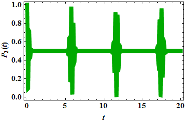
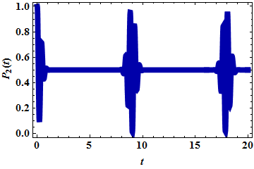
Figure 1: (Color online) The Collapse and revival phenomenon of Rabi oscillations in phosphorene for different value of wavevector angle (a) $\theta=\frac{\pi}{4}$ (b) $\theta=0$. The plot between the probability of state $\langle 0,1,n+1\mbox{ }|\phi(t)\rangle$ and time. For plotting, we considered the mean number of photon $\langle n\rangle=20$, $\lambda=1$, $u=1$, $m=1$, $v_{F}=1$ $p=1$ and $\omega=1$. Time is in the unit of $\lambda^{-1}$.

Taking initial conditions in quantized form i.e. values of the probability amplitudes are $\langle 0,1,n\mbox{ }|\phi(t)\rangle=\langle n|\alpha\rangle\;\mbox{and}\;\langle 1,0,n\mbox{ }|\phi(t)\rangle=0$, which gives

$$|\langle 0,1,n\mbox{ }|\phi(t)\rangle|^{2}=\frac{|\alpha|^{2n}}{n!}e^{-|\alpha|^{2}}.$$ (34)

Where $\alpha$ is a complex number and $|\alpha|^{2}=\langle n\rangle$ is the mean number of photons in the cavity field. The population $P_{2}(t)$ comes in form

$$P_{2P-RWA}(t)=\sum_{n}\frac{\langle n\rangle^{n}}{n!}e^{-\langle n\rangle}\cos^{2}\left(\frac{t}{2}\Omega_{\mathrm{RWA-P}}(n)\right).$$ (35)

The conventional Rabi frequency start to spread after coming Poisson distribution of the photon number $n$ in the picture. Due to Poisson distribution, there is dephasing in Rabi oscillations and collapse after some time $t$. There is revival of the collapsed comes due to the phases of oscillation of neighbouring terms in eq.(35) differ by the factor $2\pi$ dung1990collapses . The collapse and revival in Rabi oscillation can be explicitly seen by plotting $P_{2P-RWA}(t)$ with respect to time $t$ [eq.(35)]. Therefore, conventional Rabi frequency contains anisotropic nature, depicted in fig.(1). $P_{2P-RWA}(t$ has different value of amplitudes for different value of wave-vector angle $\theta$ [fig.(1)]. The detailed analysis about collapse and revival phenomenon can be seen in the book of Scully et al. scully1999quantum , the expression of collapse and revival time is derived as kumar2014quantum

$$t_{\mathrm{col}}(\bar{n})=\sqrt{\frac{2Log(10)}{\bar{n}}}\frac{\bar{n}}{\Omega_{RWA}(\bar{n})},\quad t_{\mathrm{rev}}(\bar{n})=\frac{2\pi\bar{n}}{\Omega_{RWA}(\bar{n})}.$$ (36)

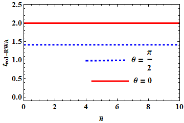
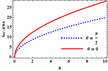
Figure 2: (Color online) For Rabi oscillations of phosphorene (a) collapse time, when wave vector angle $\theta=\frac{\pi}{2}$ and $0$. (b) revival time, when wave vector angle $\theta=\frac{\pi}{2}$ and $0$. For plotting, we considered $\lambda=1$ and $\omega=1$. Time is considered in the unit of $\lambda^{-1}$.

Therefore, in case of phosphorene final expression of of collapse and revival time for conventional Rabi frequency is

$$t_{\mathrm{col-RWA}}(\bar{n})=\sqrt{2Log(10)}\frac{1}{\lambda\sqrt{\gamma}},\quad t_{\mathrm{rev-RWA}}(\bar{n})=\frac{2\pi\sqrt{\bar{n}}}{\lambda\sqrt{\gamma}}.$$ (37)

The plot of collapse and revival time of phosphorene conventional Rabi frequency [eq.(37)] is depicted in fig.(2). The $t_{\mathrm{col}}$ is not changing with the increasing number of photon[fig.2(a)], on the other hand $t_{\mathrm{rev}}$ is changing in continuous way as number of photons increases [fig.2(b)]. But $t_{\mathrm{col}}$ and $t_{\mathrm{rev}}$ possess an anisotropic nature in phosphorene.

2.1.2 Graphene

Doing similar analogy like earlier section (2.1.1), the final equation of RWA for graphene

$$i\frac{\partial}{\partial_{t}}\langle 0,1,n+1|\phi\rangle_{2}=-\frac{\sqrt{n+1}\mbox{ }\lambda\;e^{-i\Delta_{G}t}v_{F}(p_{x}-i\;p_{y})}{2v_{F}\sqrt{p_{x}^{2}+p_{y}^{2}}}\langle 1,0,n+1|\phi_{1}\rangle_{2}$$ (38a)

$$i\frac{\partial}{\partial_{t}}\langle 1,0,n+1|\phi_{1}\rangle_{2}=-\frac{\sqrt{n+1}\;\lambda e^{i\Delta_{G}t}\mbox{ }v_{F}(p_{x}+ip_{y})}{2v_{F}\sqrt{p_{x}^{2}+p_{y}^{2}}}\langle 0,1,n+1|\phi\rangle_{2}$$ (38b)

Here $\Delta_{G}=\omega-2v_{F}\sqrt{p_{x}^{2}+p_{y}^{2}}$, which is detuning parameter in case of graphene. Applying initial condition in quantized form [like earlier section (2.1.1)], the probability amplitude of wave-function $\langle 1,0,n+1|\phi_{1}\rangle_{2}$ is

$$P_{2G-RWA}(t)=\sum_{n}\frac{\langle n\rangle^{n}}{n!}e^{-\langle n\rangle}\cos^{2}\left(\frac{t}{2}\Omega_{\mathrm{RWA-G}}(n)\right).$$ (39)

Where $\Omega_{\mathrm{RWA-G}}(n)=\sqrt{\Delta_{G}^{2}+(n+1)\lambda^{2}}$ is conventional Rabi frequency of graphene. $\Delta_{G}$ is detuning parameter, becomes zero in case of RWA. The expression of collapse and revival time kumar2014quantum for graphene is

$$t_{\mathrm{colRWA}}(\bar{n})=\sqrt{\frac{2Log(10)}{\bar{n}}}\frac{\bar{n}}{\lambda\sqrt{\bar{n}+1}},\quad t_{\mathrm{revRWA}}(\bar{n})=\frac{2\pi\bar{n}}{\lambda\sqrt{\bar{n}+1}}.$$ (40)

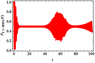
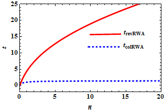
Figure 3: (Color online) The plot (a) showing isotropic nature of collapse-revival phenomenon in graphene and (b) showing collapse and revival time nature for graphene. Both plot are taken in case of conventional Rabi frequency. For plotting, we considered the mean number of photon $\langle n\rangle=20$, $\lambda=1$ and $v_{F}=1$. Time is in the unit of $\lambda^{-1}$.

The plot related with collapse-revival phenomenon [eq.(39)], collapse time $t_{\mathrm{col}}$ and revival time $t_{\mathrm{rev}}$ [eq.(40)] is depicted in fig.(3) for graphene. It can be seen in fig.3(b) that $t_{\mathrm{revRWA}}$ is not varying with number of photon, on the other hand $t_{\mathrm{colRWA}}$ is changing drastically in case of graphene.

2.2 Floquet theory approximation

2.2.1 Phosphorene

If the external driving frequency $(\omega)$ is nearly equal to the particle-hole pairs $(2v|p|)$ frequencies or resonant frequencies $(\omega_{R})$ of the system i.e. $\omega\approx\omega_{R}$ and $\omega\approx 2v|p|$, energy eigenvalue equation ($H\psi=E\psi$) are solved by using rotating wave approximation (RWA) haug2009quantum , described in earlier section(2.1). On the other hand, when $\omega$ is too large compare to the Rabi frequency $\omega_{R}$ and the resonant frequency of the creation particle-hole pairs i.e. $2v|p|$, $\omega\gg\omega_{R}$ and $\omega\gg 2v|p|$ (off-resonant case), the Floquet approximation is applied to solve energy eigenvalue equation. In Floquet theory, the Hamiltonian is decomposed in series harmonics i.e. $H=H_{0}+e^{-i\omega t}\mbox{ }V_{+}+e^{i\omega t}\mbox{ }V_{-}$. Similarly, writing wave-function in series harmonics form $\psi=\psi_{0}+e^{-i\omega t}\mbox{ }\psi_{+}+e^{i\omega t}\mbox{ }\psi_{-}$. $H_{0}$ and $\psi_{0}$ related to slow parts, on the other hand $V_{+},V_{-}$ and $\psi_{+},\psi_{-}$ related to the (coefficients of) fast parts of the full Hamiltonian and wave-function, respectively. By application of Floquet theory conditions i.e. external driving frequency $\omega$ contains larger value than band gap. Putting all these expression into energy eigenvalue equation $H\psi=E\psi$ and leaving higher harmonics i.e. order of $\frac{1}{\omega^{2}}$. Eventually, writing Hamiltonian $H$ in term of slow part only

$$H_{eff}=\left(H_{0}\mbox{ }+\frac{1}{\omega}\left[V_{-},\mbox{ }V_{+}\right]\right).$$ (41)

The Floquet oscillations frequency is eigenvalues of $H_{eff}$. Therefore, by comparison of eq.(2) with $H|\phi(t)\rangle=\left(H_{0}+e^{-i\omega t}\mbox{ }V_{+}+e^{i\omega t}\mbox{ }V_{-}\right)|\phi(t)\rangle$, the value of $H_{0}$, $V_{+}$ and $V_{-}$ will found. Therefore, Floquet energy eigenvalue equations i.e. $i\frac{\partial}{\partial_{t}}|\phi(t)\rangle=H_{eff}|\phi(t)\rangle$ have form

$$i\hbar\frac{\partial}{\partial_{t}}\langle 0,1,n+1|\phi\rangle = \left(\frac{\frac{(n+1)(2p_{y}u-v_{F})^{2}\lambda\lambda}{4v^{2}_{F}}-\frac{(n+1)(2p_{y}u+v_{F})^{2}\lambda\lambda}{4v^{2}_{F}}}{\omega}\right)\langle 0,1,n+1|\phi\rangle$$

$$+\left(up_{y}^{2}+m+ip_{x}v_{F}\right)\langle 1,0,n+1|\phi\rangle$$ (42a)

$$i\hbar\frac{\partial}{\partial_{t}}\langle 1,0,n+1|\phi\rangle = \left(\frac{\frac{(n+1)(2p_{y}u+v_{F})^{2}\lambda\lambda}{4v^{2}_{F}}-\frac{(n+1)(2p_{y}u-v_{F})^{2}\lambda\lambda}{4v^{2}_{F}}}{\omega}\right)\langle 1,0,n+1|\phi\rangle$$

$$+\left(up_{y}^{2}+m-ip_{x}v_{F}\right)\langle 0,1,n+1|\phi\rangle$$ (42b)

Therefore, the value of probability of state $\langle 1,0,n+1\mbox{ }|\phi(t)\rangle$ in polar coordinate is

$$P_{2P-Floq}(t)=|\langle 1,0,n+1\mbox{ }|\phi(t)\rangle|^{2}=\left[\frac{v_{F}^{2}\omega^{2}\beta^{2}}{v_{F}^{2}\omega^{2}\beta^{2}+4\lambda^{4}(n+1)^{2}p^{2}u^{2}\sin^{2}\theta}\right]\sin^{2}\left[t\Omega_{\mathrm{Floq}}(n)\right].$$ (43)

Where, $\beta=\sqrt{\left(m+p^{2}u\sin^{2}\theta\right)^{2}+p^{2}v_{F}^{2}\cos^{2}\theta}$ and Floquet frequency

$$\Omega_{\mathrm{Floq-P}}(n)=\sqrt{\beta^{2}+\frac{4\lambda^{4}(n+1)^{2}p^{2}u^{2}\sin^{2}\theta}{v_{F}^{2}\omega^{2}}}.$$ (44)

Choosing initial condition in quantized form like earlier section (2.1), the population $P_{2}(t)$ has form

$$P_{2P-Floq}(t)=\sum_{n}\frac{\langle n\rangle^{n}}{n!}e^{-\langle n\rangle}\left[\frac{v_{F}^{2}\omega^{2}\beta^{2}}{v_{F}^{2}\omega^{2}\beta^{2}+4\lambda^{4}(n+1)^{2}p^{2}u^{2}\sin^{2}\theta}\right]\sin^{2}\left[t\Omega_{\mathrm{Floq}}(n)\right].$$ (45)

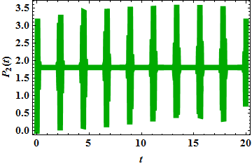
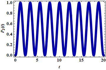
Figure 4: (Color online) The Collapse and revival phenomenon of Floquet oscillations in phosphorene for different value of wave vector angle (a) $\theta=\frac{\pi}{4}$ (b) $\theta=0$. The plot between the probability of state $\langle 0,1,n+1\mbox{ }|\phi(t)\rangle$ and time. For plotting, we considered the mean number of photon $\langle n\rangle=20$, $\lambda=1$, $u=1$, $m=1$, $v_{F}=1$ $p=1$ and $\omega=1$. Time is in the unit of $\lambda^{-1}$.

Therefore, fig.4(a) showing collapse revival phenomenon of Floquet oscillations in phosphorene, when wave-vector angle $\theta=\frac{\pi}{4}$ and collapse revival phenomenon vanished in fig.4(b), when wave-vector angle $\theta=0$. Doing similar analogy like earlier section (2.1), the expression for $t_{\mathrm{col-Floq}}$ and $t_{\mathrm{rev-Floq}}$ has form

$$t_{\mathrm{col}}(\bar{n})=\sqrt{\frac{2Log(10)}{\bar{n}}}\frac{\bar{n}}{\Omega_{\mathrm{Floq}}(\bar{n})},\quad t_{\mathrm{rev}}(\bar{n})=\frac{2\pi\bar{n}}{\Omega_{\mathrm{Floq}}(\bar{n})}.$$ (46)

The plot associated with Floquet frequency collapse and revival time [eq.(44)], given in fig.(5). From fig.(5), it can be seen that $t_{\mathrm{col-Floq}}$ and $t_{\mathrm{rev-Floq}}$ has a crucial dependency on anisotropy. For the different value of wave-vector angle $\theta$, collapse and revival time of Floquet oscillations have drastic changes.

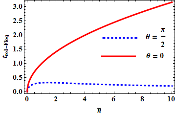
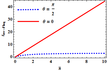
Figure 5: (Color online)For Floquet oscillations (a) collapse time, when wave vector angle $\theta=\frac{\pi}{2}$ and $0$. (b) revival time, when wave vector angle $\theta=\frac{\pi}{2}$ and $0$. For plotting, we considered $\lambda=1$ and $\omega=1$. Time is considered in the unit of $\lambda^{-1}$.

2.2.2 Graphene

Applying similar anology like earlier section (2.2.1), the graphene Floquet equations, i.e., $i\frac{\partial}{\partial_{t}}|\phi(t)\rangle=H_{eff}|\phi(t)\rangle$ have form

$$i\hbar\frac{\partial}{\partial_{t}}\langle 0,1,n+1|\phi\rangle=\frac{(n+1)\lambda^{2}}{\omega}\langle 0,1,n+1|\phi\rangle+v_{F}(p_{x}+ip_{y})\langle 1,0,n+1|\phi\rangle$$ (47a)

$$i\hbar\frac{\partial}{\partial_{t}}\langle 1,0,n+1|\phi\rangle=-\frac{(n+1)\lambda^{2}}{\omega}\langle 1,0,n+1|\phi\rangle+v_{F}(p_{x}-ip_{y})\langle 0,1,n+1|\phi\rangle$$ (47b)

Choosing initial condition in quantized form like earlier section (2.1), the population $P_{2G-Floq}(t)(=|\langle 1,0,n+1|\phi\rangle|^{2})$ has polar form

$$P_{2G-Floq}(t)=\sum_{n}\frac{\langle n\rangle^{n}}{n!}e^{-\langle n\rangle}\left[\frac{p^{2}\omega^{2}v_{F}^{2}\cos^{2}\left[t\Omega_{\mathrm{Floq-G}}(n)\right]+\lambda^{4}(n+1)^{2}}{p^{2}\omega^{2}v_{F}^{2}+\lambda^{4}(n+1)^{2}}\right].$$ (48)

The Floquet frequency $\Omega_{\mathrm{Floq-G}}(n)$ for graphene is defined as

$$\Omega_{\mathrm{Floq-G}}(n)=\sqrt{p^{2}v_{F}^{2}+\frac{\lambda^{4}(n+1)^{2}}{\omega^{2}}}$$ (49)

At Dirac point, the expression for $t_{\mathrm{colFloq}}$ and $t_{\mathrm{revFloq}}$ is

$$t_{\mathrm{colFloq}}(\bar{n})=\sqrt{\frac{2Log(10)}{\bar{n}}}\frac{\omega}{\lambda^{2}},\quad t_{\mathrm{revFloq}}(\bar{n})=\frac{2\pi\omega}{\lambda^{2}}.$$ (50)

The plot related with collapse-revival phenomenon of Floquet frequency of graphene is depicted in fig.6(a) and collapse-revival time in fig.6(b). Here $t_{\mathrm{revFloq}}$ has constant nature but $t_{\mathrm{revFloq}}$ is varying with number of photon.

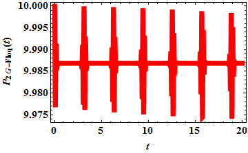
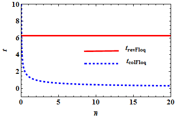
Figure 6: (Color online) The plot (a) showing isotropic nature of collapse-revival phenomenon in graphene and (b) showing collapse and revival time nature for graphene. Both plot are taken in case of Floquet frequency. For plotting, we considered the mean number of photon $\langle n\rangle=20$, $\lambda=1$, $\omega=1$ and $v_{F}=1$. Time is in the unit of $\lambda^{-1}$.

The plot showing anisotropic nature of Floquet frequency in phosphorene is depicted in fig.7(a) and compare between Floquet frequency of phosphorene [eq.(44)] and graphene [eq.(49)] is depicted in fig.7(b). The value of Floquet frequency of phosphorene is much larger than graphene at Dirac point (p=0), can be explicitly seen in fig.7(b). Such threshold value of Floquet frequency comes due to the gap $m$ acting as the Dirac mass.

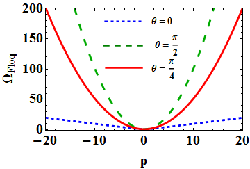
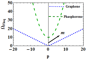
Figure 7: (Colour Online) (a) Shows the Floquet frequency with respect to momentum in phosphorene for different values of wave vector angle $\theta$, which shows the anisotropic behaviour. (b) Comparison of Floquet frequency in phosphorene $(\theta=\frac{\pi}{4})$ and graphene. For plotting, we have taken $\lambda=0.1$, $\omega=1$, $n=10$ and $v_{F}=1$. All parameters are taken in the unit of $\omega^{-1}$.

The valence-conduction band tuning of phosphorene via Floquet frequency, can be seen in fig. (8). The band gap has been reduced, when external electromagnetic field has applied [fig.8(b)]. Therefore, the Floquet frequency is a good tool for band tuning of 2D materials.

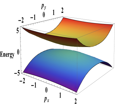
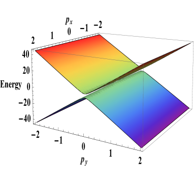
Figure 8: (Color online) The 3D plot (a) is showing energy vs momentum diagram without detuning i.e. in the absence of the external field (eigenvalues of $H_{0}$). The 3D plot (b) is showing energy vs momentum, when detuning of the external field comes in the picture (eigenvalues of $H_{eff}$). For plotting, we have taken $\lambda=1$, $v_{F}=1$, $u=1$, $m=1$, $n=10$, and $\omega=10$ (parameters are plotted in unit of $\omega^{-1}$).

3 Quantum Bloch-Seigert shift

3.1 Phosphorene

By using RWA, the expression for conventional Rabi frequency $\Omega_{\mathrm{RWA}}(n)$ [from section (2.1.1)] is

$$\Omega_{\mathrm{RWA-P}}(n)=\sqrt{\Delta_{p}^{2}+(n+1)\lambda^{2}\gamma}$$ (51)

Where $\Delta_{p}=(\omega-2\beta)$ is detuning parameter, $\beta$ and $\gamma$ by considering momentum vector in polar form i.e. $p_{x}=p\cos\theta$, $p_{y}=p\sin\theta$ and $\hbar=1$, is defined as

$$\beta=\sqrt{\left(m+p^{2}u\sin^{2}\theta\right)^{2}+p^{2}v_{F}^{2}\cos^{2}\theta}$$

$$\gamma=\frac{\left[\left(m+p^{2}u\sin^{2}\theta\right)^{2}+p^{4}u^{2}\sin^{2}2\theta\right]}{\left(m+p^{2}u\sin^{2}\theta\right)^{2}+p^{2}v_{F}^{2}\cos^{2}\theta}$$

The condition in RWA, the external frequency should equal to the frequency of two-level systems. Therefore, the counter-rotating terms are neglected haug2009quantum . But RWA becomes invalid in the strong driving regimes, due to presence of counter-rotating terms. Therefore, a shift in conventional Rabi frequency resonance condition comes, known as Bloch-Siegert shift (BSS) bloch1940magnetic . The expression of the conventional Rabi frequency with BSS

$$\Omega_{\mathrm{RWA-P-BSS}}(n)=\sqrt{\left(\Delta-\frac{\gamma\lambda^{2}(n+1)}{8\beta}\right)^{2}+\lambda^{2}(n+1)\gamma-\left(\frac{\gamma\lambda^{2}(n+1)}{8\beta}\right)^{2}}$$ (52)

The term $\frac{\gamma\lambda^{2}(n+1)}{8\beta}$ is shift in conventional Rabi frequency, called as BSS . BSS is depending on the wave-vector angle $\theta$, so its nature becomes anisotropic in phosphorene.

3.2 Graphene

Similarly, the expression for conventional Rabi frequency for graphene [from section (2.1.2)] is

$$\Omega_{\mathrm{RWA-G}}(n)=\sqrt{\Delta_{G}^{2}+(n+1)\lambda^{2}}$$ (53)

Here $\Delta_{G}=\omega-2v_{F}\sqrt{p_{x}^{2}+p_{y}^{2}}$, which is detuning parameter in case of graphene. In presence of BSS, the conventional Rabi frequency have form

$$\Omega_{RWA-G-BSS}=\sqrt{(n+1)\lambda^{2}-\frac{(n+1)\lambda^{2}}{64p^{2}}+\left(\Delta-\frac{(n+1)\lambda^{2}}{8p}\right)^{2}}$$ (54)

Therefore, isotropic nature of graphene conventional Rabi frequency BSS can be seen from above expression eq.(54). The term $\frac{(n+1)\lambda^{2}}{8p}$ is shift in conventional Rabi frequency, called as BSS in graphene.

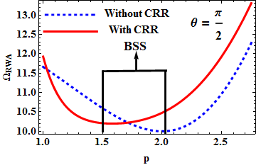
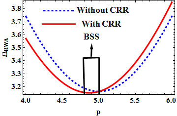
Figure 9: (Color online) Plot (a) BSS in phosphorene corresponds to $\theta=\frac{\pi}{2}$. Plot (b) BSS in graphene, independent on wave vector $\mathrm{\theta}$. CRR is abbreviation of counter rotating term. For plotting, we considered, $\lambda=1$, $u=1$, $m=1$, $v_{F}=1$ $p=1$ $n=9$ and $\omega=10$. Parameters are taken in unit of in the unit of $\lambda^{-1}$.

In case of zero photon limit, i.e., $n=0$, in eq.(51) and eq.(52), the Rabi oscillation is found. Such phenomenon is known as vacuum Rabi oscillation. The BSS in case of phosphorene is depicted in the fig.9(a) and for graphene in the fig.9(b). So BSS contains anisotropic nature in phosphorene.

4 Anisotropy of Quantum Floquet Oscillations via Numerical Model in Phosphorene

For explicitly justifying role of anisotropy in quantum Floquet oscillation of phosphorene, the numerical solution of Floquet-Bloch equations have been described. From these equations, it can be seen clearly that wave-vector angle $\theta$ plays a major role in quantum Floquet oscillation of phosphorene. For phosphorene, the Floquet-Bloch equations are

$$i\hbar\frac{\partial}{\partial_{t}}\langle 0,1,n+1|\phi\rangle = \left[\left\{up^{2}_{y}+m\right\}+iv_{F}p_{x}\right]\mbox{ }\langle 1,0,n+1|\phi\rangle+e^{-i\omega t}\left[\left\{-i\frac{2up_{y}}{2v_{F}}\lambda\mbox{ }\right\}-\frac{i}{2}\lambda\right]\;\sqrt{n+1}\mbox{ }$$ (55a)

$$\langle 1,0,n+1|\phi\rangle+e^{i\omega t}\left[\left\{i\frac{2up_{y}}{2v_{F}}\lambda\mbox{ }\right\}-\frac{i}{2}\lambda\right]\;\sqrt{n+1}\mbox{ }\langle 1,0,n+1|\phi\rangle$$

$$i\hbar\frac{\partial}{\partial_{t}}\langle 1,0,n+1|\phi\rangle = \left[\left\{\left(up^{2}_{y}\right)+m\right\}-iv_{F}p_{x}\right]\mbox{ }\mbox{ }\langle 0,1,n+1|\phi\rangle+e^{-i\omega t}\left[\left\{-i\frac{2up_{y}}{2v_{F}}\lambda\right\}+\frac{i}{2}\lambda\right]\;\sqrt{n+1}\mbox{ }$$ (55b)

$$\langle 0,1,n+1|\phi\rangle+e^{i\omega t}\left[i\left\{\frac{2up_{y}}{2v_{F}}\lambda\right\}+\frac{i}{2}\lambda\right]\mbox{ }\sqrt{n+1}\mbox{ }\langle 0,1,n+1|\phi\rangle$$

Where we have taken $n\approx n+1$ and $\lambda=1$. By using NDSolve routine in Mathematica software Mathematica , the eq.(55a) and eq.(55b) solved numerically and shown in fig.(10). The time period belongs to Floquet frequencies is described in table (1), which is showing anisotropic nature and verifying the time period of analytical Floquet frequency (eq.(44)). As we increase value of $p$, the time period of Floquet oscillations decreasing continuously irrespective of the value of $\theta$ (table (1)). Therefore, it can be said that, anisotropy is a crucial and significant parameter for Floquet oscillations in phosphorene.

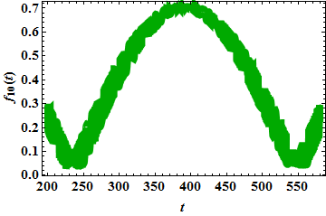
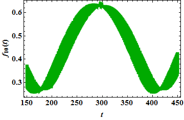
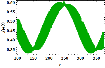
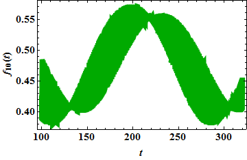
Figure 10: (Color online) Time period (T) of oscillations in plot (a) corresponds to Floquet frequency with a period of 312.6 (b) corresponds to Floquet frequency with a period of 236.77 (c) corresponds to Floquet frequency with a period of 198.25 (d) corresponds to Floquet frequency with a period of 173.95. For plotting, we have taken $n=99$, $p=0.01$, $v_{F}=1$, $u=1$, $m=.001$, $\lambda=1$ and $\omega=100$. Parameters are considered in the unit of $\lambda^{-1}$.

$\huge p$	T$|_{\theta=0}$	T$|_{\theta=\pi/6}$	T$|_{\theta=\pi/4}$	T$|_{\theta=\pi/3}$
$0.01$	312.6	236.77	198.25	173.95
$0.02$	156.88	118.64	99.27	87.07
$0.03$	104.66	79.12	66.19	58.06
$0.04$	78.51	59.35	49.65	43.54
0.05	62.82	47.48	39.72	34.83

Table 1: Time period (T) of oscillations for various values of $\mathrm{\theta}$, confirming the anisotropic behaviour of Floquet oscillations in phashphorene. T is in the units of $\lambda^{-1}$.

5 Conclusions

We have described, how anisotropy is playing major role in Floquet theory and rotating wave approximation in case of phosphorene. Floquet theory becomes important in case of low energy physics, so in the low energy region, the band tuning of phosphorene can be done via Floquet frequency. There is no role of anisotropy in case graphene. The results of Floquet frequency and Rabi frequency are compared between graphene and phosphorene, wherever required. But, Floquet theory becomes more important in case of low energy physics. Therefore, Floquet theory is an important tool for the study of the 2D materials.

References

- (1) Z.W. Li, Y.H. Hu, Y. Li, Z.Y. Fang, Chinese Physics B 26(3), 036802 (2017)
- (2) K.S. Novoselov, A.K. Geim, S.V. Morozov, D. Jiang, Y. Zhang, S.V. Dubonos, I.V. Grigorieva, A.A. Firsov, science 306(5696), 666 (2004)
- (3) A.H.C. Neto, F. Guinea, N.M. Peres, K.S. Novoselov, A.K. Geim, Reviews of modern physics 81(1), 109 (2009)
- (4) Z.H. Ni, T. Yu, Y.H. Lu, Y.Y. Wang, Y.P. Feng, Z.X. Shen, ACS nano 2(11), 2301 (2008)
- (5) M.Y. Han, B. Özyilmaz, Y. Zhang, P. Kim, Physical review letters 98(20), 206805 (2007)
- (6) H. Liu, A.T. Neal, Z. Zhu, Z. Luo, X. Xu, D. Tománek, P.D. Ye, ACS nano 8(4), 4033 (2014)
- (7) M. Ezawa, in Journal of Physics: Conference Series, vol. 603 (IOP Publishing, 2015), vol. 603, p. 012006
- (8) Z. Guo, H. Zhang, S. Lu, Z. Wang, S. Tang, J. Shao, Z. Sun, H. Xie, H. Wang, X.F. Yu, P.K. Chu, Adv. Funct. Mater. 25(7486), 6996 (2015)
- (9) J. Yang, R. Xu, J. Pei, Y.W. Myint, F. Wang, Z. Wang, S. Zhang, Z. Yu, Y. Lu, Light: Science and Applications 4(4), 1 (2015)
- (10) D. Li, J.R. Xu, K. Ba, N. Xuan, M. Chen, Z. Sun, Y.Z. Zhang, Z. Zhang, 2D Materials 4(3), 031009 (2017)
- (11) L. Viti, M.S. Vitiello, arXiv preprint arXiv:1804.11262 (2018)
- (12) J. Eberly, L. Allen, Optical resonance and two-level atoms (John Wiley & Sons, 1975)
- (13) H. Haug, S.W. Koch, Quantum theory of the optical and electronic properties of semiconductors (World Scientific Publishing Co Inc, 2009)
- (14) C. Gerry, P. Knight, Introductory Quantum Optics (Cambridge University Press., 2005)
- (15) Z. Ni, H. Wang, J. Kasim, H. Fan, T. Yu, Y. Wu, Y. Feng, Z. Shen, Nano letters 7(9), 2758 (2007)
- (16) L. Mandel, E. Wolf, Optical coherence and quantum optics (Cambridge university press, 1995)
- (17) R.W. Boyd, Nonlinear optics (Academic Press, New York, 2008)
- (18) P.A. Lee, Physical review letters 71(12), 1887 (1993)
- (19) A.W. Ludwig, M.P. Fisher, R. Shankar, G. Grinstein, Physical Review B 50(11), 7526 (1994)
- (20) K. Ziegler, Physical review letters 80(14), 3113 (1998)
- (21) R.R. Nair, P. Blake, A.N. Grigorenko, K.S. Novoselov, T.J. Booth, T. Stauber, N.M. Peres, A.K. Geim, Science 320(5881), 1308 (2008)
- (22) S. Kumar, M. Anija, N. Kamaraju, K. Vasu, K. Subrahmanyam, A. Sood, C. Rao, Applied physics letters 95(19), 191911 (2009)
- (23) M. Breusing, S. Kuehn, T. Winzer, E. Malić, F. Milde, N. Severin, J. Rabe, C. Ropers, A. Knorr, T. Elsaesser, Physical Review B 83(15), 153410 (2011)
- (24) J.M. Dawlaty, S. Shivaraman, M. Chandrashekhar, F. Rana, M.G. Spencer, Applied Physics Letters 92(4), 042116 (2008)
- (25) J. Shang, Z. Luo, C. Cong, J. Lin, T. Yu, G.G. Gurzadyan, Applied Physics Letters 97(16), 163103 (2010)
- (26) P.A. George, J. Strait, J. Dawlaty, S. Shivaraman, M. Chandrashekhar, F. Rana, M.G. Spencer, Nano letters 8(12), 4248 (2008)
- (27) B.A. Ruzicka, L.K. Werake, H. Zhao, S. Wang, K.P. Loh, Applied Physics Letters 96(17), 173106 (2010)
- (28) X. Wang, S. Lan, Advances in Optics and Photonics 8(4), 618 (2016)
- (29) X. Wang, A.M. Jones, K.L. Seyler, V. Tran, Y. Jia, H. Zhao, H. Wang, L. Yang, X. Xu, F. Xia, Nature Nanotechnology 10(7486), 1 (2017)
- (30) L. Miao, B. Shi, J. Yi, Y. Jiang, C. Zhao, S. Wen, Scientific Reports 7(3352), 517 (2017)
- (31) V.A. Margulis, E.E. Muryumin, E.A. Gaiduk, Eur. Phys. J. B 90(90), 203 (2017)
- (32) Y. Xu, X.F. Jiang, Y. Ge, Z. Guo, Z. Zeng, Q.H. Xu, H. Zhang, X.F. Yu, D. Fan, J. Mater. Chem. C 5(90), 3007 (2017)
- (33) T.G. Pedersen, Phys. Rev. B 95(90), 235419 (2017)
- (34) I.I. Rabi, Physical Review 51(8), 652 (1937)
- (35) L. Allen, J. Eberly, Optical Resonances and Two-Level Atoms, lnterscience Monographs and Texts in Physics and Astronomy 28 (Wiley, New York, 1975)
- (36) M. Lindberg, S.W. Koch, Physical Review B 38(5), 3342 (1988)
- (37) T. Oka, H. Aoki, Physical Review B 79(8), 081406 (2009)
- (38) N.H. Lindner, G. Refael, V. Galitski, Nature Physics 7(6), 490 (2011)
- (39) T. Kitagawa, T. Oka, A. Brataas, L. Fu, E. Demler, Physical Review B 84(23), 235108 (2011)
- (40) J. Inoue, Phys. Rev. Lett. 105, 017401 (2010)
- (41) B. Dóra, J. Cayssol, F. Simon, R. Moessner, Physical review letters 108(5), 056602 (2012)
- (42) M. Ezawa, Physical review letters 110(2), 026603 (2013)
- (43) Enamullah, V. Kumar, G.S. Setlur, Physica B: Condensed Matter 407(23), 4600 (2012)
- (44) F. Bloch, A. Siegert, Physical Review 57(6), 522 (1940)
- (45) S.A. Vierkötter, Journal of Magnetic Resonance, Series A 118(1), 84 (1996)
- (46) M. Beijersbergen, R. Spreeuw, L. Allen, J. Woerdman, Physical Review A 45(3), 1810 (1992)
- (47) U. Kumar, V. Kumar, Enamullah, G.S. Setlur, JOSA B 31(12), 3042 (2014)
- (48) S. Fukuoka, T. Taen, T. Osada, Journal of the Physical Society of Japan 84(12), 121004 (2015)
- (49) U. Kumar, V. Kumar, et al., Physica E: Low-dimensional Systems and Nanostructures 108, 288 (2019)
- (50) J.H. Shirley, Physical Review 138(4B), B979 (1965)
- (51) S. Stenholm, Journal of Physics B: Atomic and Molecular Physics 5(4), 878 (1972)
- (52) P. Hannaford, D. Pegg, G. Series, Journal of Physics B: Atomic and Molecular Physics 6(8), L222 (1973)
- (53) C. Cohen-Tannoudji, J. Dupont-Roc, C. Fabre, Journal of Physics B: Atomic and Molecular Physics 6(8), L214 (1973)
- (54) E.T. Jaynes, F.W. Cummings, Proceedings of the IEEE 51(1), 89 (1963)
- (55) H.I. Yoo, J.H. Eberly, Physics Reports 118(5), 239 (1985)
- (56) F.W. Cummings, Physical Review 140, A1051 (1965)
- (57) J.H. Eberly, N. Narozhny, J. Sanchez-Mondragon, Physical Review Letters 44(20), 1323 (1980)
- (58) N. Narozhny, J. Sanchez-Mondragon, J. Eberly, Physical Review A 23(1), 236 (1981)
- (59) H. Yoo, J. Sanchez-Mondragon, J. Eberly, Journal of Physics A: Mathematical and General 14(6), 1383 (1981)
- (60) Z. Ficek, M.R. Wahiddin, Quantum optics for beginners (CRC Press, 2014)
- (61) L.V. Vela-Arevalo, R.F. Fox, Physical Review A 71(6), 063403 (2005)
- (62) B.T. Torosov, S. Longhi, G. Della Valle, Optics Communications 346, 110 (2015)
- (63) Enamullah, V. Kumar, U. Kumar, G.S. Setlur, JOSA B 31(3), 484 (2014)
- (64) H.T. Dung, R. Tanaś, A. Shumovsky, Optics communications 79(6), 462 (1990)
- (65) M.O. Scully, M.S. Zubairy, Quantum optics (Cambridge University Press, page(201-202), 1999)
- (66) W.R. Inc. Mathematica, Version 11.1. Champaign, IL, 2017