Resilience of Traffic Networks with Partially Controlled Routing

Abstract

This paper investigates the use of Infrastructure-To-Vehicle (I2V) communication to generate routing suggestions for drivers in transportation systems, with the goal of optimizing a measure of overall network congestion. We define link-wise levels of trust to tolerate the non-cooperative behavior of part of the driver population, and we propose a real-time optimization mechanism that adapts to the instantaneous network conditions and to sudden changes in the levels of trust. Our framework allows us to quantify the improvement in travel time in relation to the degree at which drivers follow the routing suggestions. We then study the resilience of the system, measured as the smallest change in routing choices that results in roads reaching their maximum capacity. Interestingly, our findings suggest that fluctuations in the extent to which drivers follow the provided routing suggestions can cause failures of certain links. These results imply that the benefits of using Infrastructure-To-Vehicle communication come at the cost of new fragilities, that should be appropriately addressed in order to guarantee the reliable operation of the infrastructure.

I Introduction

Transportation systems are fundamental components of modern smart cities, and their effective and reliable operation are critical aspects to guarantee the development of quickly-growing metropolitan areas. Recent advances in vehicle technologies, such as Infrastructure-To-Vehicle (I2V) communication and Vehicle-To-Vehicle (V2V) communication [1], set out an enormous potential to overcome the inefficiencies of traditional transportation systems. Notwithstanding, the development efficient control algorithms capable of effectively engaging these capabilities is an extremely-challenging task due to the tremendous complexity of the interconnections [2], that often results in suboptimal performance [3], and that can potentially generate novel fragilities [4, 5].

In this paper, we discuss the use of I2V communication to partially influence the routing decisions of the drivers, with the goal of optimizing a measure of overall network congestion. We define link-wise levels of trust to tolerate the non-cooperative behavior of a certain ratio of the drivers, and we develop an optimization-based control mechanism to provide real-time routing suggestions based on the current state congestion levels. Differently from traditional approaches for network routing design, our methods allow us to take into account quickly-varying traffic volumes, and do not require the knowledge of the traffic demands associated with every origin-destination pair. Moreover, we study the impact of changes in routing that result in roads reaching their maximum capacity, thus leading to traffic jams or cascading failure effects. We develop a technique to classify the links based on their resilience, and we study the fragility of the network against changes in routing. Surprisingly, our findings demonstrate that networks where the routing is partially controlled by a system planner can be more fragile to traffic jam phenomena as compared to networks where drivers perform traditional selfish routing choices.

Related Work Routing decisions of traditional human drivers are non-cooperative, namely, drivers act as a group of distinct agents that make selfish routing decisions with the goal of minimizing their individual delay [6]. The inefficiencies of such noncooperative behavior are often quantified through the price of anarchy [7, 8, 9], a measure that captures the cost of suboptimality with respect to the societal optimal efficiency. The availability of V2V and I2V has recently demonstrated the potential to influence the traditional behavior of drivers in a transportation system [3, 10]. In particular, the control of the routing choices was proposed as a promising solution to improve the efficiency of the network [10] and to enhance its resilience [11]. Differently from this line of previous work, this paper focuses on systems operating at non-equilibrium points, on tolerating the presence of non-cooperative driver behaviors, and on characterizing the impact of controlled routing on the resilience of the system.

Contribution The contribution of this paper is fourfold. First, we formulate and solve an optimization problem to design optimal routing suggestions with the goal of minimizing the travel time experienced by all network users. The optimization problem incorporates link-wise trust parameters that describe the extent to which drivers on that link are willing to follow the suggested routing policy. Second, we develop an online update scheme that takes into account instantaneous changes in the levels of trust on the provided routing suggestions. Discrepancies between the modeled and actual trust parameters can be the result of quickly varying traffic demands, or can be the effect of selfish routing decisions. Third, we study the resilience of the network, measured as the smallest change in the trust parameters that results in roads reaching their maximum capacity. We present an efficient technique to approximate the resilience of the network links, and we discuss how these quantities can be computed from the output of the optimization problem. Fourth, we demonstrate through simulations that, although partially controlling the routing may improve the travel time for all network users, it also results in increased network fragility due to possible fluctuations in the trust parameters.

Organization The rest of this paper is organized as follows. Section II describes the dynamical network framework, and formulates the problem of optimal network routing with varying levels of trust. Section III presents a method to numerically solve the optimization, and illustrates our real-time update mechanism. Section IV is devoted to the study and characterization of the network resilience, while Section V presents simulations results to validate our methods. Finally, Section VI concludes the paper.

II Problem Formulation

We model a traffic network with a directed graph $\mathcal{G}=(\mathcal{V},\mathcal{E})$, where $\mathcal{V}=\{1,\dots,m\}$ denotes the set of nodes, and $\mathcal{E}=\{1,\dots,n\}\subseteq\mathcal{V}\times\mathcal{V}$ denotes the set of edges. Nodes of the graph identify traffic junctions, while edges identify sections of roads (links) that interconnect two junctions. An element $(i,j)\in\mathcal{E}$ denotes a directed link from node $j$ to node $i$. We associate to every link $i\in\mathcal{E}$ a dynamical equation of the form

$$\dot{x}_{i}={f}^{\textup{in}}_{i}(x,t)-{f}^{\textup{out}}_{i}(x,t),$$

where $t\in\mathbb{R}_{\geq 0}$, $x_{i}:\mathbb{R}_{\geq 0}\rightarrow\mathbb{R}_{\geq 0}$ denotes the traffic density of link $i$, and ${f}^{\textup{in}}_{i}(x,t)$ and ${f}^{\textup{out}}_{i}(x,t)$ denote the inflow and outflow of the link, respectively. We assume that vehicle inflows enter the network at on-ramp links ${\mathcal{E}}^{\textup{on}}$, while vehicle outflows exit the network at off-ramp links ${\mathcal{E}}^{\textup{off}}$. We denote by ${\mathcal{E}}^{\textup{in}}$ the set of internal links that are connected through junctions, and assume that ${\mathcal{E}}^{\textup{on}}$, ${\mathcal{E}}^{\textup{off}}$, and ${\mathcal{E}}^{\textup{in}}$ are disjoint sets, with $\mathcal{E}={\mathcal{E}}^{\textup{on}}\cup{\mathcal{E}}^{\textup{off}}\cup{\mathcal{E}}^{\textup{in}}$ (see Fig. 1 for an illustration). The network topology described by $\mathcal{G}$ imposes natural constraints on the dynamics of the links, where flow is possible only between links that are interconnected by a node. We associate to every pair of links a turning ratio $r_{ij}\in[0,1]$, describing the fraction of vehicles entering link $i\in\mathcal{E}$ after exiting $j\in\mathcal{E}$. We combine the drivers turning preferences into a matrix $R=[r_{ij}]\in{}^{n\times n}$, where

$$r_{ij}\in[0,1], r_{ij}\neq 0\text{ only if }(i,j)\in\mathcal{E}.$$ (1)

The conservation of flows at the junctions imposes the following constraints on the entries of $R$:

$$\sum_{i}r_{ij}=1,\text{ for all }j\in\mathcal{E}\setminus{\mathcal{E}}^{\textup{off}},$$

$$\sum_{i}r_{ij}=0,\text{ for all }j\in{\mathcal{E}}^{\textup{off}}.$$ (2)

We let $\mathcal{R}_{\mathcal{G}}$ be the set of matrices

$$\mathcal{R}_{\mathcal{G}}=\{R=[r_{ij}]\in{}^{n\times n}\;:\;r_{ij}\text{ satisfy \eqref{eq:Rentries} and }\eqref{eq:RrowSum}\},$$

and let $n_{r}=\|R\|_{0}$ denote the number of nonzero entries in matrix $R$. We assume that the vehicles routing is partially controllable, and denote by $\sigma_{i}:\mathbb{R}_{\geq 0}\rightarrow[0,1]$ the ratio of controllable vehicles that instantaneously occupy link $i$. For every $i\in\mathcal{E}$, we assume that a fraction $(1-\sigma_{i})$ of vehicles leaving $i$ will follow a selfish route choice ${r}^{\textup{s}}_{ij}$, for all $j\in\mathcal{E}$, while the remaining vehicles can be routed according to the routing decisions made by a system planner, namely ${r}^{\textup{c}}_{ij}$. The parameter $\sigma_{i}$ can be interpreted as the (average) extent to which drivers follow the routing suggestion ${r}^{\textup{c}}_{ij}$. We combine the selfish and controllable routing parameters into matrices ${R}^{\textup{S}}\in{}^{n\times n}$ and ${R}^{\textup{C}}\in{}^{n\times n}$, respectively, and decompose the matrix of turning preferences as

$$R=\Sigma{R}^{\textup{C}}+(I-\Sigma){R}^{\textup{S}},$$

where $\Sigma$ is a diagonal matrix $\Sigma=\operatorname{Diag}(\sigma_{1},\dots,\sigma_{n})$. Note that the graph topology and sparsity pattern of $R$ impose the following constraints on ${R}^{\textup{S}}$ and ${R}^{\textup{C}}$:

$${R}^{\textup{S}}\in\mathcal{R}_{\mathcal{G}}, {R}^{\textup{C}}\in\mathcal{R}_{\mathcal{G}}.$$

We stress that in this work ${R}^{\textup{C}}$ is a design parameter containing the set of routing suggestions provided by the system planner to influence the drivers routing choices.

Remark 1

(Selfish Route Choices) Typically, the selfish behavior of drivers is captured by a Wardrop equilibrium [6], that is, a configuration in which the travel time associated to any source-destination path chosen by a nonzero fraction of the drivers does not exceed the travel time associated to any other path. We remark that, in our settings, such equilibrium configuration is captured by the selfish routing matrix ${R}^{\textup{S}}$. $\square$

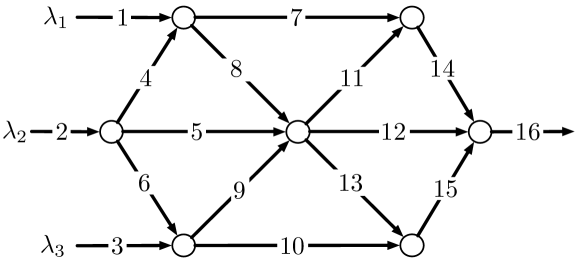
Figure 1: Example of traffic network interconnection. For this network, ${\mathcal{E}}^{\textup{on}}=\{1,2,3\}$, ${\mathcal{E}}^{\textup{in}}=\{4,\dots,15\}$, and ${\mathcal{E}}^{\textup{off}}=\{16\}$.

We adopt Daganzo’s Cell Transmission Model [12], and model the physical characteristic of each link by a demand function $d_{i}(x_{i})$ and a supply function $s_{i}(x_{i})$, that represent upper bounds on the outflow and inflow of each link, respectively:

$${f}^{\textup{in}}_{i}(x,t)\leq s_{i}(x_{i}), {f}^{\textup{out}}_{i}(x,t)\leq d_{i}(x_{i}).$$ (3)

For every link $i\in\mathcal{E}$ we let $B_{i}:=\sup\{x:s_{i}(x)>0\}$ denote its saturation density, which corresponds to the jam density of the road. We model on-ramps $i\in{\mathcal{E}}^{\textup{on}}$ as links with infinite supply functions $s_{i}(x_{i})=+\infty$, and denote by $\lambda_{i}(t)$ the corresponding inflow rate. Then, road inflows and outflows are related by means of the following equations

$${f}^{\textup{in}}_{i}(x,t)=\begin{cases}\lambda_{i}(t),&i\in{\mathcal{E}}^{\textup{on}},\\ \sum_{j}r_{ij}{f}^{\textup{out}}_{j}(x,t),&i\in\mathcal{E}\setminus{\mathcal{E}}^{\textup{on}},\\ \end{cases}$$ (4)

which capture the conservation of flows at the junctions. We model the outflows from the links as

$${f}^{\textup{out}}_{i}(x,t)=\kappa_{i}(x)d_{i}(x_{i}),$$ (5)

where $\kappa_{i}(x)\in[0,1]$ is a parameter that enforces the bounds (3) or, in other words, guarantees that every outgoing link has adequate supply to accommodate the demand of its incoming links. Different models for $\kappa_{i}(x)$ have been proposed in the literature, and prevalent roles have been played by FIFO policies [13] and proportional allocation rules [14]. We combine the link dynamical equations with (4) and (5) to derive the overall network dynamics

$$\dot{x}=(R-I){f}^{\textup{}}(x,t)+\lambda,$$ (6)

where $I\in{}^{n\times n}$ is the identity matrix, $x=[x_{1}~{}\dots~{}x_{n}]^{\mathsf{T}}$ is the vector of link densities, ${f}^{\textup{}}=[{f}^{\textup{out}}_{1}~{}\dots~{}{f}^{\textup{out}}_{n}]^{\mathsf{T}}$ is the vector of link outflows, and $\lambda=[\lambda_{1}~{}\dots~{}\lambda_{n}]^{\mathsf{T}}$ denotes the vector of exogenous inflows, where we let $\lambda_{i}=0$ if $i\not\in{\mathcal{E}}^{\textup{on}}$.

We consider the network performance measured by the Total Travel Time (TTT),

TTT $$:=\int_{0}^{\mathcal{H}}x_{1}(t)+\dots+x_{n}(t)~{}dt,$$

which is a measure of the delay experienced by all users [15], and we focus on the problem of designing the matrix of turning preferences in a way that

$$\min_{{R}^{\textup{C}}}\;\;\;\;\;\;\;\;\;$$ TTT

subject to $$\dot{x}=(R-I){f}^{\textup{}}(x,t)+\lambda,$$ (7a)

$$R=\Sigma{R}^{\textup{C}}+(I-\Sigma){R}^{\textup{S}},$$ (7b)

$${R}^{\textup{C}}\in\mathcal{R}_{\mathcal{G}},$$ (7c)

$$x\leq B,$$ (7d)

where $\mathcal{H}$ is the control horizon, $x(0)=x_{0}$ is the (given) network initial configuration, and $B=[B_{1}\dots B_{n}]^{\mathsf{T}}$ denotes the vector of jam densities. From a real-time control and implementation perspective, solving (7) sets out a number of challenges. First, the length of the optimization horizon $\mathcal{H}$ is a fundamental parameter that should be accurately chosen. One should chose $\mathcal{H}$ adequately large to include all relevant system dynamics, but unnecessarily large values of $\mathcal{H}$ can drastically increase the computational burden. Second, rapid changes in traffic volumes and driver preferences require the development of control mechanisms that are capable to adapt in real-time to sudden variations of $\sigma$. In fact, the performance of the optimization strongly depends on $\sigma$, and fluctuations in this parameter can lead to considerable variability in network performance and efficiency.

To study the effects of fluctuations in $\sigma$, in the second part of this paper we consider the problem of quantifying the fragility of the network against changes in the trust levels that result in links reaching their jam density. We assume that a link irreversibly fails if it reaches its jam density, and argue that such failure may propagate in the network and potentially cause a cascading failure effect. We measure the network resilience $\rho(\mathcal{G},x_{0})$ as the $L^{1}$-norm of the smallest variation in $\sigma$ that results in such failure phenomena, that is,

$$\rho(\mathcal{G},x_{0}):=\;\;\;\;\;\min_{\tilde{\sigma}}\;\;\;\;\;\;\;\;\; \|\tilde{\sigma}-\sigma\|_{1}$$

such that $$\dot{x}=(R-I){f}^{\textup{}}(x,t)+\lambda,$$

$$R=\Sigma{R}^{\textup{C}}+(I-\Sigma){R}^{\textup{S}},$$

$$x_{i}\geq B_{i},$$

where $x(0)=x_{0}$, $t\in[0,\mathcal{H}]$, and $i\in\{1,\dots,n\}$.

III Design of the Turning Preferences

In this section we present a method to numerically solve the optimization problem (7), and illustrate an online-update technique to address the control challenges outlined above.

III-A Computing Optimal Routing Suggestions

We begin by recasting the optimization problem (7) in a way that allows us to numerically compute its solutions. We perform three simplifying steps, described next.

First, in order to generate a tractable prediction of the time evolution of the network state, we discretize (6) by means of the Euler discretization technique. We use a sampling time $T_{s}\in{}_{>0}$ that is chosen to guarantee the Courant-Friedrichs-Lewy assumption $\max_{i}\frac{v_{i}T_{s}}{L_{i}}\leq 1$ for all links [12], where $v_{i}\in\mathbb{R}_{\geq 0}$ and $L_{i}\in{}_{>0}$ denote the maximum speed and the length of the section of road, respectively. Let $\operatorname{vec}\left(R\right)=[r_{11}\dots r_{n1}~{}r_{12}\dots r_{nn}]$ denote the vectorization of matrix $R=[r_{ij}]$, and let $t_{k}=kT_{s}$, $k\in\mathbb{N}$. Then, the time-evolution of (6) from $t_{k}$ to $t_{k+1}=t_{k}+T_{s}$ can be discretized as

$$x_{k+1}=x_{k}+T_{s}((R_{k}-I)f(x_{k})+\lambda_{k}):=\mathcal{F}(x_{k},r_{k},\lambda_{k}),$$ (8)

where $r_{k}=\operatorname{vec}\left(R_{k}\right)$. We remark that the dependency on time of the routing matrix is the result of time-varying $\sigma$.

Second, we vectorize equation (7b) and let

$$r_{k}=(\Sigma_{k}^{\mathsf{T}}\otimes I){r}^{\textup{c}}+((I-\Sigma_{k})^{\mathsf{T}}\otimes I){r}^{\textup{s}}:=\Psi(\sigma_{k},{r}^{\textup{s}},{r}^{\textup{c}}),$$

where ${r}^{\textup{c}}=\operatorname{vec}\left({R}^{\textup{C}}\right)$, ${r}^{\textup{s}}=\operatorname{vec}\left({R}^{\textup{S}}\right)$, the symbol $\otimes$ denotes the Kronecker product, and where we used the identity $\operatorname{vec}\left(AXB\right)=(B^{\mathsf{T}}\otimes A)\operatorname{vec}\left(X\right)$ for matrices $A$, $X$, and $B$ of appropriate dimensions.

Third, we observe that the Euler discretization technique employed in (8) preserves the sparsity pattern of ${R}^{\textup{C}}$, and we rewrite the sparsity constraints (7c) as

$$\sum_{i}r_{ij}^{\text{c}}=b_{j}, 0\leq{r_{ij}}^{\textup{\!\!\!\!\!c}}\leq 1, \;\;\;(i,j)\in\mathcal{E},$$

where $b_{j}=1$ if $j\in\mathcal{E}\setminus{\mathcal{E}}^{\textup{off}}$, and $b_{j}=0$ if $j\in{\mathcal{E}}^{\textup{off}}$.

Finally, we recast the optimization problem (7) by using the discretized dynamics as

$$\min_{{r}^{\textup{c}}}\;\;\;\;\;\;\;\;\; \sum_{k=1}^{h}\mathds{1}^{\mathsf{T}}x_{k}$$

subject to $$x_{k+1}=\mathcal{F}(x_{k},r_{k},\lambda_{k}), k=1,\dots,h,$$ (9a)

$$r_{k}=\Psi(\sigma_{k},{r}^{\textup{s}},{r}^{\textup{c}}), k=1,\dots,h,$$ (9b)

$$\sum_{i}r_{ij}=b_{j}, j=1,\dots,n,$$ (9c)

$$0\leq{r_{ij}}^{\textup{\!\!\!\!\!c}}\leq 1, (i,j)\in\mathcal{E},$$ (9d)

$$x_{k}\leq B, k=1,\dots,h,$$ (9e)

where $\mathds{1}\in{}^{n}$ denotes the vector of all ones, and $h$ and $T_{s}$ are chosen so that $hT_{s}=\mathcal{H}$. As discussed in e.g. [16], the constraints (9a) are often nonconvex in the decision variables. Thus, the optimization problem (9) is of the form of a nonconvex nonlinear programming optimization problem, over $n_{r}=\|R\|_{0}$ decision variables, and can be solved numerically through common nonlinear optimization solvers, such as interior-point methods [17].

III-B Online Update Mechanism

In order to take into account for the quick variability of the parameter $\sigma$ and to deal with the considerable computational effort required to determine the solution to (9), we propose an adaptive control scheme that generates real-time updates based on the instantaneous changes in $\sigma$. The proposed adaptive mechanism is outlined in Fig. 2, and is structured as follows. We assume that a central processing unit is in charge of computing $R^{\text{C}*}(\sigma_{0})$, that is, the solution to the optimization problem (9) with a given (fixed) set of trust parameters $\sigma_{0}$. The underlying choice for $\sigma_{0}$ can reflect the current network conditions, or can be dictated by the availability of historical data. Moreover, we assume that the solution $R^{\text{C}*}(\sigma_{0})$ is intermittently made available at time instants $t=kT_{c}$, where $T_{c}\in{}_{>0}$ is the time required to solve the optimization. We are interested in constructing an efficient mechanism to determine $R^{\text{C}*}(\sigma)$, the optimal solution to (9) with the instantaneous value of $\sigma$, by updating $R^{\text{C}*}(\sigma_{0})$.

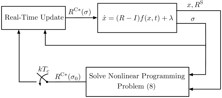
Figure 2: Real-time update scheme.

Our online update method is motivated by the fact that $\sigma$ is subject to small variations from the nominal value $\sigma_{0}$. In fact, the following inequality follows from (1)

$$\|\sigma-\sigma_{0}\|\leq\|[1\cdots 1]^{\mathsf{T}}\|=\sqrt{n_{r}}.$$

Next, we derive our online update mechanism. We denote in compact form by

$$f_{0}({r}^{\textup{c}},\hat{x},\sigma)=\sum_{k=1}^{h}\mathds{1}^{\mathsf{T}}x_{k},\quad g({r}^{\textup{c}},\hat{x},\sigma)=\begin{bmatrix}{r_{ij}}^{\textup{\!\!\!\!\!c}}-1\\ -{r_{ij}}^{\textup{\!\!\!\!\!c}}\\ x_{k}-B\end{bmatrix},$$

$$h({r}^{\textup{c}},\hat{x},\sigma)=\begin{bmatrix}x_{k+1}-\mathcal{F}(x_{k},r_{k},\lambda_{k})\\ r_{k}-\Psi(\sigma,{r}^{\textup{s}},{r}^{\textup{c}})\\ \sum_{i}r_{ij}-b_{j}\end{bmatrix},$$

where $\hat{x}=[x_{1}^{\mathsf{T}}\dots x_{h}^{\mathsf{T}}]^{\mathsf{T}}\in{}^{nh}$ denotes the joint vector of model-prediction variables, and rewrite (9) as

$$\min_{{r}^{\textup{c}}}\;\;\;\;\;\;\;\;\; f_{0}({r}^{\textup{c}},\hat{x},\sigma)$$

subject to $$g_{i}({r}^{\textup{c}},\hat{x},\sigma)\leq 0, i\in\{1,\dots,q\},$$

$$h_{j}({r}^{\textup{c}},\hat{x},\sigma)=0, j\in\{1,\dots,p\},$$ (10)

where we have made explicit the dependency of the optimization problem on the decision variables ${r}^{\textup{c}}$, on the prediction variables $\hat{x}$, and on the parameter $\sigma$. To characterize the solutions to (10), we compose the Lagrangian

$$\mathcal{L}({r}^{\textup{c}},\hat{x},\sigma,w,u)=f_{0} ({r}^{\textup{c}},\hat{x},\sigma)+$$

$$u^{\mathsf{T}}g({r}^{\textup{c}},\hat{x},\sigma)+w^{\mathsf{T}}h({r}^{\textup{c}},\hat{x},\sigma),$$

where $u=[u_{1}\dots u_{q}]^{\mathsf{T}}$ and $w=[w_{1}\dots w_{p}]^{\mathsf{T}}$ are the vectors of Lagrange Multipliers, and we write the first order Karush-Kuhn-Tucker (KKT) conditions:

$$\nabla\mathcal{L}(r^{\text{c}*},\hat{x}^{*},\sigma_{0},w^{*},u^{*})=0,$$

$$u_{i}g_{i}(r^{\text{c}*},\hat{x}^{*},\sigma_{0})=0,$$

$$h_{j}(r^{\text{c}*},\hat{x}^{*},\sigma_{0})=0,$$

with the additional inequalities $u_{i}^{*}\geq 0$, and $g_{i}(r^{\text{c}*},\hat{x}^{*},\sigma_{0})\leq 0$, where $\nabla=[\partial/\partial r^{\text{c}}_{1}\dots\partial/\partial r^{\text{c}}_{n_{r}}]^{\mathsf{T}}$ denotes the gradient operator with respect to the decision variables ${r}^{\textup{c}}$. We denote the set of KKT equality conditions in compact form as

$$F(r^{\text{c}*},\hat{x}^{*},\sigma_{0},u^{*},w^{*})=0,$$ (11)

and note that (11) is an implicit equation that characterizes the optimal solutions to (10). Finally, by letting $y=[{r}^{\textup{c}}(\sigma)~{}u(\sigma)~{}w(\sigma)]$ and by assuming that (11) holds for $\sigma$ near $\sigma_{0}$, we compute the total derivative of the implicit function (11) with respect to $\sigma$ to obtain the following relationship that holds at optimality:

$$M(\sigma)\frac{dy}{d\sigma}+N(\sigma)=0,$$

where the matrices $M(\sigma)=[\partial F_{i}/\partial y_{j}]$, $dy/d\sigma=[dy_{i}/d\sigma_{j}]$, and $N(\sigma)=[\partial F_{i}/\partial\sigma_{j}]$. Finally, to formalize our online update rule we make the following classical assumption (see e.g. [18]), which guarantees: (i) that $r^{\text{c}*}$ is a local isolated minimizing point, (ii) the uniqueness of the Lagrange Multipliers, and (iii) the invertibility of matrix $M(\sigma_{0})$.

Assumption III.1

(Second Order Minimizer Point)

(Second-order KKT conditions) The inequality $v^{\mathsf{T}}\nabla^{2}\mathcal{L}(r^{\text{c}*},\hat{x}^{*},\sigma,w^{*},u^{*})v>0$ holds for every vector $v\in{}^{n+m+p}$, $v\neq 0$, that satisfies

$$v^{\mathsf{T}}\nabla g_{i}(r^{\text{c}*},\hat{x}^{*},\sigma_{0}) \leq 0,\text{ for all $i$ where }u_{i}^{*}=0,$$

$$v^{\mathsf{T}}\nabla g_{i}(r^{\text{c}*},\hat{x}^{*},\sigma_{0}) =0,\text{ for all $i$ where }u_{i}^{*}>0,$$

$$v^{\mathsf{T}}\nabla h(r^{\text{c}*},\hat{x}^{*},\sigma_{0}) =0.$$

(Constraints independence) The vectors $\nabla g(r^{\text{c}*},\hat{x}^{*},\sigma_{0})$ and $\nabla h(r^{\text{c}*},\hat{x}^{*},\sigma_{0})$ are linearly independent.

(Strict complementary slackness) If $g_{i}(r^{\text{c}*},\hat{x}^{*},\sigma_{0})=0$, then $u_{i}^{*}>0$. $\square$

Lemma III.2

(Linear Update Rule) Let Assumption III.1 hold, let $r^{\text{c}*}(\sigma_{0})$ denote a solution to (9) with $\sigma=\sigma_{0}$, and let $\eta:=M^{-1}(\sigma_{0})N(\sigma_{0})$ be partitioned as

$$\eta=\begin{bmatrix}\eta_{1}\\ \eta_{2}\\ \eta_{3}\end{bmatrix},$$

where $\eta_{1}\in{}^{n_{r}\times n}$, $\eta_{2}\in{}^{q\times n}$, and $\eta_{3}\in{}^{p\times n}$. Then,

$$r^{\text{c}*}(\sigma)=r^{\text{c}*}(\sigma_{0})+\eta_{1}(\sigma-\sigma_{0})+o(\|\sigma-\sigma_{0}\|^{2}).$$ (12)

We argue that the update (12) can be computed through simple vector multiplications, and thus is significantly more efficient than solving (9). The accuracy of the linear approximation rule is numerically validated in Fig. 3, which demonstrates the quadratic decay of the approximation error as $\sigma$ approaches $\sigma_{0}$ (see Section V for a thorough discussion).

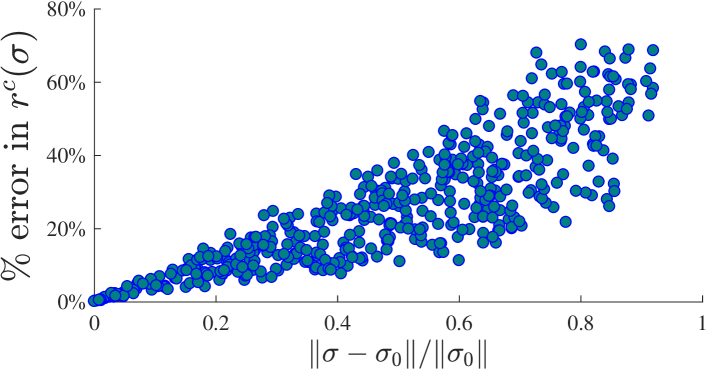
Figure 3: Numerical validation of the update rule (12).

IV Network Resilience

In this section, we study the resilience of the network against changes in the degrees of trust of the drivers, and we illustrate a technique that allows us to classify the links in relation to their resilience properties. We start with the following definition of margin of resilience of a network link.

Definition 1

(Links Margin of Resilience) Let $i\in\mathcal{E}$, and let $B_{i}$ be its jam density. The margin of resilience of link $i$ is

$$\rho_{i}(x_{0}):=\;\;\;\;\;\min_{\sigma}\;\;\;\;\;\;\;\;\; \|\sigma-\sigma_{0}\|_{1}$$

such that $$\dot{x}=(R-I){f}^{\textup{}}(x,t)+\lambda,$$

$$R=\Sigma{R}^{\textup{C}}+(I-\Sigma){R}^{\textup{S}},$$

$$x_{i}\geq B_{i},\text{ for some }t\in[0,\mathcal{H}].$$

$\square$

In other words, the resilience of a certain link is defined as the smallest change in $\sigma$ that generates its jam failure. Next, we present a lower bound on the margin of resilience of the links. Our approach is based on the real-time control rule (12), and on first-order approximations of the constraints.

Theorem IV.1

(Lower Bound on Margin of Resilience) Let $i\in\mathcal{E}$, let $\mathcal{F}(x_{k},r_{k},\lambda_{k})=[\mathcal{F}_{1}(x_{k},r_{k},\lambda_{k})\dots\mathcal{F}_{n}(x_{k},r_{k},\lambda_{k})]^{\mathsf{T}}$, and let

$$\Psi_{i}(r_{k},x_{k},\lambda_{k},\sigma):=\frac{\partial\mathcal{F}_{i}(x_{k},r_{k},\lambda_{k})}{\partial\sigma}+\frac{\partial\mathcal{F}_{i}(x_{k},r_{k},\lambda_{k})}{\partial{r}^{\textup{c}}}~{}\eta_{1},$$

where $\eta_{1}$ is defined in (12). Then,

$$\rho_{i}(x_{0})\geq\min_{k}\frac{B_{i}-\mathcal{F}_{i}(x_{k},r_{k},\lambda_{k})}{\left\|\Psi_{i}(k,\lambda,\sigma_{0})\right\|_{\infty}}.$$

Proof:

We first recast the notion of margin of resilience in terms of the discretized system (9). The margin of resilience of link $i$ is the smallest change $\|\sigma-\sigma_{0}\|_{1}$ such that

$$\mathcal{F}_{i}(x_{k},r_{k}(\sigma),\lambda_{k})\geq B_{i},$$ (13)

for some $k\in\{1,\dots,h\}$. We then rewrite $\mathcal{F}_{i}(x_{k},r_{k}(\sigma),\lambda_{k})$ by taking its Taylor expansion for around $\sigma_{0}$

$$\mathcal{F}_{i}(x_{k},r_{k}( \sigma),\lambda_{k})=\mathcal{F}_{i}(x_{k},r_{k}(\sigma_{0}),\lambda_{k})+$$

$$\underbrace{\left.\frac{d\mathcal{F}_{i}}{d\sigma}(x_{k},r_{k}(\sigma),\lambda_{k})\right|_{\sigma=\sigma_{0}}}_{\Psi_{i}(r_{k},x_{k},\lambda_{k},\sigma)}\delta_{\sigma}+o(\|\delta_{\sigma}\|^{2}),$$

where $\delta_{\sigma}=\sigma-\sigma_{0}$, and where we used the implicit differentiation rule to compute $\Psi_{i}(r_{k},x_{k},\lambda_{k},\sigma)=\frac{\partial\mathcal{F}_{i}}{\partial\sigma}+\frac{d\mathcal{F}_{i}}{d{r}^{\textup{c}}}\;\frac{d{r}^{\textup{c}}}{d\sigma}$, with ${d{r}^{\textup{c}}}/{d\sigma}=\eta_{1}$. By substituting into (13) and by rearranging the terms we obtain

$$B_{i}-\mathcal{F}_{i}(x_{k},r_{k}(\sigma_{0}), \lambda_{k})+o(\|\delta_{\sigma}\|^{2})\leq\Psi_{i}(r_{k},x_{k},\lambda_{k},\sigma)\delta_{\sigma}.$$

Finally, we take the $L^{1}$-norm on both sides of the above inequality, which yields

$$|B_{i} -\mathcal{F}_{i}(x_{k},r_{k}(\sigma_{0}),\lambda_{k})+o(\|\delta_{\sigma}\|^{2})|$$

$$\leq\left|\Psi_{i}(r^{\text{c}},x_{k},\lambda_{k},\sigma)\delta_{\sigma}\right|\leq\left\|\Psi_{i}(r^{\text{c}},x_{k},\lambda_{k},\sigma)\right\|_{\infty}\left\|(\delta_{\sigma})\right\|_{1}$$

where we used Holder’s inequality [19]. To conclude, we iterate the above reasoning for all times $k\in\{1,\dots,h\}$, which yields the given bound for the margin of resilience and concludes the proof. ∎

We conclude this section by observing that the quantity $\Psi_{i}(r_{k},x_{k},\lambda_{k},\sigma)$ is also a constraint of (9), and thus can be directly computed from the output of the optimization. The tightness of the bound and the implications of the theorem are discussed in the next section.

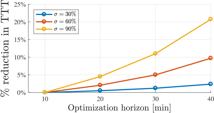
Figure 4: Travel time reduction for degrees of trust and optimization horizons.

V Simulation Results

This section provides numerical simulations in support to the assumptions made in this paper, and includes discussions and demonstrations of the benefits of the proposed methods. We consider the network shown in Fig. 1, which comprises $n=16$ links and $m=7$ nodes. Each link has capacity $B_{i}=B=200\text{veh}$, length $L_{i}=L=5.25\text{mi}$, and velocity $v_{i}=v=35\text{mi/h}$. For all $i$, we let $d_{i}(x_{i})=v(1-\text{exp}(-ax_{i}))$, $a=0.01$, and $s_{i}(x_{i})=\frac{v}{L}(B-x_{i})$ be the link demand and supply functions, respectively, and choose $\kappa_{i}(x)$ according to a proportional allocation rule [14]. We let $T_{s}=0.15\text{h}$, and observe that $\max_{i}\frac{vT_{s}}{L}=1$ satisfies the Courant-Friedrichs-Lewy assumption [12]. We let the network inflows be $\lambda_{i}=10\text{veh/min}$ for all $i\in\mathcal{E}^{\textup{on}}$, and assume that the density of the each link at time $t=0$ is $100\text{veh/mi}$, for all $i\in\mathcal{E}$. The selfish turning preferences are chosen so that $r^{\text{s}}_{ij}$ is split uniformly between the outgoing links at every node. Moreover, we assume $\sigma_{i}=\sigma$ for all $i$.

We begin by evaluating the benefits of partially controlling the network routing. Fig. 4 illustrates the reduction in Total Travel Time in relation to different trust levels. The figure highlights that a consistent reduction in Total Travel Time is the combined result of significant levels of trust in the provided routing suggestions and of considerably-large control horizons. Next, we investigate the network resilience in relation to changes in $\sigma$ (Fig. 5 and 6). To this aim, we show in Fig. 5 the distance from jam density of every link in the network when drivers follow non-cooperative routing (i.e. $\sigma=0$). Formally, this quantity is captured by the link residual capacity

$$\text{RC}_{i}:=\min_{k}\;\frac{B_{i}-\mathcal{F}_{i}(x_{k},r_{k},\lambda_{k})}{B_{i}},$$

which is a measure of the distance between the link density over time and its jam density $B_{i}$. Note that, for the considered case study, all links operate with less than $30\%$ of their residual capacity. The lower bound on the links margin of resilience (Theorem IV.1) is show in Fig. 6. Two important implications follow from the simulation results illustrated in Fig. 6. First, the trends observed in the figure support our observation that partially controlling the routing can result in increased fragility. In fact, $\rho_{i}(x_{0})$ for $\sigma_{0}=0$ is strictly larger that $\rho_{i}(x_{0})$ for $\sigma_{0}=30\%$ for all $i\in\{4,\dots 16\}\setminus\{5,12\}$. Second, values of $\rho_{i}(x_{0})$ greater than $100\%$ (observed, for instance, on link $i=16$) imply that no feasible change in $\sigma$ can lead to a jam failure of that link, while values of $\rho_{i}(x_{0})<100\%$ imply that there exists a feasible perturbation in $\sigma$ that results in jam-failures of that link. We note that the values reported in Fig. 6 are consistent with the considered network topology. In fact, the dynamics of link $i=16$ are independent of the routing choices performed by the drivers in the rest of the network.

VI Conclusions

This paper proposes a real-time optimization framework to design routing suggestions with the goal of optimizing the travel time experienced by all users in dynamical transportation systems that operate at non-equilibrium points. Our framework allows us to quantify the reduction in Total Travel Time in relation to different levels of trust on the provided routing suggestions, and to design a technique to study the resilience of the network links against fluctuations in the trust levels. Our results reveal a tradeoff between efficiency and resilience in a transportation system, demonstrating that partially controlling the routing can reduce the margin of resilience of certain links. Interesting aspects that require further investigation include extending the findings to more general network topologies, and the design of incentive mechanisms to regulate and control the trust parameters.

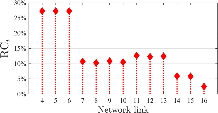
Figure 5: Links distance from constraint violation (non-cooperative routing).

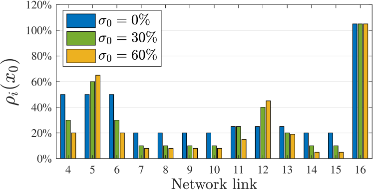
Figure 6: Lower bound on links margin of resilience.

References

- [1] C. Wu, A. Kreidieh, E. Vinitsky, and A. M. Bayen, “Emergent behaviors in mixed-autonomy traffic,” in Conference on Robot Learning, 2017, pp. 398–407.
- [2] G. Bianchin and F. Pasqualetti, “A network optimization framework for the analysis and control of traffic dynamics and intersection signaling,” in IEEE Conf. on Decision and Control, Miami, FL, Dec. 2018.
- [3] D. A. Lazar, S. Coogan, and R. Pedarsani, “The price of anarchy for transportation networks with mixed autonomy,” in American Control Conference, Jul. 2018, pp. 6359–6365.
- [4] V. Bonifaci, T. Harks, and G. Schäfer, “Stackelberg routing in arbitrary networks,” Mathematics of Operations Research, vol. 35, no. 2, pp. 330–346, 2010.
- [5] G. Bianchin and F. Pasqualetti, Time-Delay Attacks in Network Systems. Springer International Publishing, 2018, pp. 157–174.
- [6] J. G. Wardrop, “Some theoretical aspects of road traffic research,” Proceedings of the institution of civil engineers, vol. 1, no. 3, pp. 325–362, 1952.
- [7] T. Roughgarden and É. Tardos, “How bad is selfish routing?” Journal of the Association for Computing Machinery, vol. 49, no. 2, pp. 236–259, 2002.
- [8] J. R. Correa, A. S. Schulz, and N. E. Stier-Moses, “Selfish routing in capacitated networks,” Mathematics of Operations Research, vol. 29, no. 4, pp. 961–976, 2004.
- [9] G. Perakis, “The “price of anarchy” under nonlinear and asymmetric costs,” Mathematics of Operations Research, vol. 32, no. 3, pp. 614–628, 2007.
- [10] D. A. Lazar, S. Coogan, and R. Pedarsani, “Capacity modeling and routing for traffic networks with mixed autonomy,” in IEEE Conf. on Decision and Control, Dec. 2017, pp. 5678–5683.
- [11] G. Como, K. Savla, D. Acemoglu, M. A. Dahleh, and E. Frazzoli, “Robust distributed routing in dynamical networks—part I: Locally responsive policies and weak resilience,” IEEE Transactions on Automatic Control, vol. 58, no. 2, pp. 317–332, 2013.
- [12] C. F. Daganzo, “The cell transmission model part II: network traffic,” Transp. Research Part B: Methodological, vol. 29, no. 2, pp. 79–93, 1995.
- [13] S. Coogan and M. Arcak, “A compartmental model for traffic networks and its dynamical behavior,” IEEE Transactions on Automatic Control, vol. 60, no. 10, pp. 2698–2703, 2015.
- [14] E. Lovisari, G. Como, and K. Savla, “Stability of monotone dynamical flow networks,” in IEEE Conf. on Decision and Control, Dec. 2014, pp. 2384–2389.
- [15] G. Gomes and R. Horowitz, “Optimal freeway ramp metering using the asymmetric cell transmission model,” Transp. Research Part C: Emerging Technologies, vol. 14, no. 4, pp. 244–262, 2006.
- [16] A. Hegyi, B. De Schutter, and H. Hellendoorn, “Model predictive control for optimal coordination of ramp metering and variable speed limits,” Transp. Research Part C: Emerging Technologies, vol. 13, no. 3, pp. 185–209, 2005.
- [17] A. Wächter and L. T. Biegler, “On the implementation of an interior-point filter line-search algorithm for large-scale nonlinear programming,” Mathematical programming, vol. 106, no. 1, pp. 25–57, 2006.
- [18] A. V. Fiacco and G. P. McCormick, Nonlinear programming: sequential unconstrained minimization techniques. SIAM, 1990, vol. 4.
- [19] G. H. Hardy, J. E. Littlewood, and G. Pólya, Inequalities. Cambridge University Press, 1988.