Offspring Population Size Matters when Comparing Evolutionary Algorithms with Self-Adjusting Mutation Rates

Abstract

We analyze the performance of the 2-rate $(1+\lambda)$ Evolutionary Algorithm (EA) with self-adjusting mutation rate control, its 3-rate counterpart, and a $(1+\lambda)$ EA variant using multiplicative update rules on the OneMax problem. We compare their efficiency for offspring population sizes ranging up to $\lambda=3,200$ and problem sizes up to $n=100,000$.

Our empirical results show that the ranking of the algorithms is very consistent across all tested dimensions, but strongly depends on the population size. While for small values of $\lambda$ the 2-rate EA performs best, the multiplicative updates become superior for starting for some threshold value of $\lambda$ between 50 and 100. Interestingly, for population sizes around 50, the $(1+\lambda)$ EA with static mutation rates performs on par with the best of the self-adjusting algorithms.

We also consider how the lower bound $p_{\min}$ for the mutation rate influences the efficiency of the algorithms. We observe that for the 2-rate EA and the EA with multiplicative update rules the more generous bound $p_{\min}=1/n^{2}$ gives better results than $p_{\min}=1/n$ when $\lambda$ is small. For both algorithms the situation reverses for large $\lambda$.

1 Introduction

A key driver for the success of evolutionary algorithms (EAs) is their global search behavior, i.e., their capability of searching the whole decision space without getting stuck in local optima. This feature distinguishes EAs from other well-known heuristics such as Simulated Annealing and other local hill climbers, which search the decision space only within a small neighborhood. The global search behavior of EAs, however, comes at the cost of a less focused search when the optimization converges, which can result in performances losses in the final parts of the optimization process. The question how to most effectively combine the best of both worlds is the driving force behind research on parameter control [KHE15, AM16, EHM99], adaptive operator selection [MLS10, FCSS10], and hyper-heuristics [BGH⁺13], which are the most prominent umbrella terms for adjusting the structure of the search behavior to the current needs of an iterative optimization process.

Interestingly, research on parameter control has shown that in many applications the search behavior can be adjusted very efficiently by quite simple update rules, see the above-cited surveys for details. The considerable performance gains observed in practice have inspired a whole series of theoretical works on non-static parameter choices. In the last years, an increasing number of results appeared which rigorously quantify the advantages of parameter control, see [DD18b] for a summary and classification of the mechanisms.

We will focus in this work on two different self-adjusting approaches previously shown to yield excellent performances on the OneMax benchmark problem: a 2-rate success control and a generalized one-fifth success rule. We analyze their efficiency when implemented in a $(1+\lambda)$ EA framework. Our key research question concerns the scalability of performance with respect to the offspring population size $\lambda$ and with respect to the problem dimension $n$. A summary of findings will be presented in Section 1.2.

1.1 Self-Adjusting Algorithms

The One-Fifth Success Rule Applied to the $(1+\lambda)$ EA. The one-fifth success rule originally stems from theoretical observations made by Rechenberg for the optimal step-size adaptation in the (1+1) Evolution Strategy [Rec73]. An interpretation of this rule which is suitable also for the adaptation of other parameters, such as the mutation rate in discrete EAs, was presented in [KMH⁺04]. The rule itself is simple: if after one iteration of an algorithm a strictly better offspring has been found, the parameter under consideration is multiplied with some constant $F$, and it is multiplied with $F^{-1/4}$ otherwise. With this setting it holds that after 5 iterations the parameter is the same as in the first if exactly one out of the five iterations was “successful” (i.e., found a better solution), and it is increased or decreased otherwise, depending on the sign of $1-F$ and the number of successful iterations. The one-fifth success rule was shown to yield very efficient optimization times for the $(1+(\lambda,\lambda))$ Genetic Algorithm (GA), first by empirical means [DDE15] and later by rigorous mathematical running time analysis [DD18a].

Since the one-fifth success rule had been derived only for the (1+1) ES and only for particular benchmark problems (the sphere and a corridor function [Rec73]), it seems natural to generalize the update mechanisms to other success rules. In fact, multiplying the parameters by $2$ and $1/2$ in the case of a successful and an unsuccessful iteration, respectively, has been experimented with in various context. It has also been rigorously proven to be efficient for the optimization of different benchmark functions with a $(1+\lambda)$ EA variant that uses a self-adjusting offspring population size $\lambda$ [LS11]. In [DW18] an empirical study analyzed the impact of the update factors on the performance of a (1+1) EA variant. This algorithm samples in each iteration one offspring $y$ from the current best solution $x$ and updates the mutation rate $p$ to $bp$ (with $b<1$ being some constant) if $y$ is at least as good as its parent (i.e., in our setting with maximization as objective, if and only if $f(y)\geq f(x)$). In this situation $x$ is replaced by $y$. If $y$ is strictly worse than $x$ (i.e., if $f(y)<f(x)$) the mutation rate is increased to $Ap$, where $A>1$ is again some constant. The results presented in [DW18] show that this self-adjusting $(1+1)~{}\text{EA}(A,b)$ is very efficient on two classic benchmark problems OneMax and LeadingOnes, and this holds for broad ranges of update strengths $A$ and $b$. In the very recent work [DDL19] it was rigorously proven that this algorithm, for suitably chosen hyper-parameters $A$ and $b$, achieves optimal optimization time on LeadingOnes, up to lower order terms.

In this work, we will extend the $(1+1)~{}\text{EA}(A,b)$ to the $(1+\lambda)$ EA, which samples $\lambda$ offspring per each iteration. Since the probability of creating individuals which are equally good, but not strictly better than the parent, increases considerably for large $\lambda$, we have to refine the interpretation of “success” for this context. Taking into account that the fraction of offspring $y$ satisfying $f(y)\geq f(x)$ showed promising performances in initial experiments, in our $(1+\lambda)$ EA$(A,b)$ we therefore discriminate with respect to whether or not at least $5\%$ of the offspring are at least as good as their parent.

2-Rate and 3-Rate Update Rules. An alternative way to control the mutation rate was proposed and analyzed in [DGWY19]. Their 2-rate $(1+\lambda)$ EA, which we refer to as 2-rate $(1+\lambda)$ EA_r/2,2r in the following, uses two different mutation rates in each iteration. Half the offspring are created with mutation rate $p/2$ and the other $\lambda/2$ offspring are sampled with mutation rate $2p$. The mutation rate is parametrized as $p=r/n$ in the 2-rate $(1+\lambda)$ EA_r/2,2r. The value of $r$ is updated after each iteration, by a random decision which favors the rate by which the best offspring has been created (details will be presented in Section 2). It was proven in [DGWY19] that the 2-rate $(1+\lambda)$ EA_r/2,2r with $\lambda\geq 45$ and $\lambda=n^{O(1)}$ is not only more efficient for the optimization of OneMax than any $(1+\lambda)$ EA with static mutation rates, but, from a comparison with a lower bound proven in [BLS14], their result also implies that the 2-rate $(1+\lambda)$ EA_r/2,2r even achieves asymptotically optimal expected optimization time, which is $\Theta\left(\frac{n}{\log\lambda}+\frac{n\log n}{\lambda}\right)$ when measured in terms of generations.

We also study a 3-rate variant of 2-rate $(1+\lambda)$ EA_r/2,2r, which creates one third of the offspring with mutation rate $c_{1}r/n$, $r/n$, and $c_{2}r/n$, respectively, where $0<c_{1}<1$ and $1<c_{2}$ are hyper-parameters set by the user. In the original work [DGWY19] a similar 3-rate variant has been studied by empirical means. We extend their preliminary study by considering 100 different pairs of $(c_{1},c_{2})$, but also by considering its performance for a broader range of population sizes $\lambda$ and much larger dimensions $n$.

1.2 Summary of Results

We investigate the efficiency of the three above-mentioned algorithms (i.e., the $(1+\lambda)$ EA$(A,b)$, the 2-rate $(1+\lambda)$ EA_r/2,2r, and the 3-rate $(1+\lambda)$ EA_r/2,r,2r) on OneMax, for various population sizes $\lambda$ up to 3,200 and problem sizes up to $n=100{,}000$. Their performances are compared among each other and to the traditional $(1+\lambda)$ EA using static mutation rates.

Interestingly, the ranking of the algorithms is very consistent across all tested dimensions, and only depends on the offspring population size $\lambda$. More precisely, we show that for small population sizes $\lambda\leq 50$, the 2-rate $(1+\lambda)$ EA_r/2,2r performs best, while for $\lambda\geq 100$ the $(1+\lambda)$ EA$(A,b)$ is the most efficient among the four algorithms. It is also worth mentioning that for $\lambda$ of about 50, the conventional $(1+\lambda)$ EA with static mutation rates performs on par with the best performing self-adjusting algorithm, which is 2-rate $(1+\lambda)$ EA_r/2,2r.

All our algorithms are implemented with the shift mutation operator discussed in [CD18b]. This operator, unlike the unconditional standard bit mutation operator traditionally studied in the theory of evolutionary computation, ensures that offspring differ from their parent by at least one bit. This is achieved as follows. The operator first draws the mutation strength $\ell$ (i.e., the number of bits that are flipped to create the offspring) from the binomial distribution $\operatorname{Bin}(n,p)$, where the parameter $p$ denotes the mutation rate. While the traditional standard bit mutation operator allows $\ell=0$, it is easily seen that, for $(1+\lambda)$ EAs, which only evolve a single solution, an offspring that is identical to its parent cannot advance the search. The shift mutation operator therefore interprets $\ell=0$ as a vote for a small search radius, and flips exactly one bit, i.e., effectively using $\ell=1$. Put differently, this operator always flips at least one bit, and its probability of flipping exactly one bit equals $\operatorname{Bin}(n,p)(0)+\operatorname{Bin}(n,p)(1)$.

When the mutation rate $p$ converges to zero, the shift mutation operator converges against the operator using mutation strength one deterministically, thus effectively reducing the global search property of standard bit mutation to a purely local search. As explained above, we would like to avoid performing a purely random search only, and therefore cap the mutation rate at a lower bound $p_{\min}.$ This lower bound can have a significant impact on the performance, as our further experimental results demonstrate. More precisely, we observe that for smaller population sizes a lower bound of $1/n^{2}$ seems to work better than a lower bound of $1/n$. Interestingly, the situation reverses for larger population sizes. These observations are true for all considered self-adjusting algorithms, but with different values of $\lambda$. For 2-rate $(1+\lambda)$ EA_r/2,2r, the transition population size is between $\lambda=100$ and $\lambda=200$, while for $(1+\lambda)$ EA$(A,b)$ it is between $\lambda=400$ and $\lambda=800$.

In light of the consistent behavior across all tested dimensions, we are confident that our findings will inspire future rigorous theoretical analyses for the self-adjusting algorithms investigated herein.

1.3 Related Work

Our work can, to some extent, be seen as an extension of [DYvR⁺18], where different $(1+\lambda)$ EA variants have been studied on the two benchmark problems OneMax and LeadingOnes. Note though that we consider here much larger offspring population sizes $\lambda$ (up to $3,200$) and much larger dimensions (up to $100{,}000$), whereas the results presented in [DYvR⁺18] are restricted to settings with $n\leq 4000$, and $\lambda\in\{1,2,5,10,50\}$. As discussed above, the ranking of the algorithms strongly depends on the size of $\lambda$, so that our work gives a much more complete picture than the results presented in [DYvR⁺18].

1.4 Structure of the Paper

The rest of the paper is structured as follows. In Section 2 we describe the considered algorithms in more detail. Section 3 gives a general overview of how each algorithm performs across different dimensions and population sizes. In Section 4 the influence of the lower bound for the mutation probability is studied, and conclusions about the ranking of the self-adjusting algorithms are made. Section 5 provides insights into the anytime performance of the algorithms from the fixed-budget perspective. In Section 6 we compare the 2-rate $(1+\lambda)$ EA_r/2,2r with its 3-rate counterpart. Conclusions and avenues for future work are presented in Section 7.

2 OneMax and Three $(1+\lambda)$ EA Variants

In this section we describe the baseline $(1+\lambda)$ EA_0→1 algorithm and its two self-adjusting variants. The description of the algorithms assumes the maximization of a pseudo-Boolean function $f:\{0,1\}^{n}\rightarrow\mathbb{R}$ as the optimization task. All empirical results in the further sections are obtained for the OneMax benchmark problem $\textsc{Om}:\{0,1\}^{n}\to\mathbb{R},x\mapsto\sum_{i=1}^{n}{x_{i}}$. OneMax is the most widely studied benchmark problem in the theory of EAs [Jan13, AD11], but also serves as a recurring benchmark problem in empirical studies, and in particular in the context of parameter control [FCSS08, Bäc92, Bäc93, JDJW05, DW18]. A discussion of properties that make OneMax a suitable test problem for adaptive algorithms was offered by Thierens in [Thi09]. Apart from the better comparison with existing results, the availability of theoretical performance limits of adaptive and static evolutionary algorithms makes OneMax a particularly appealing benchmark problem; see [Doe18] for a survey of such black-box complexity bounds. In the context of our work, the asymptotic $\Theta\big{(}\frac{n}{\log\lambda}+\frac{n\log n}{\lambda}\big{)}$ bound for all $\lambda$-parallel EAs proven in [BLS14] and the precise $n\ln(n)-cn\pm o(n)$ bound for any unary unbiased black-box algorithm from [DDY16] are the probably most relevant results. As mentioned at the end of Section 1.2, we are also confident that further advances in running time analysis will allow us to convert our empirical findings into rigorous mathematical statements.

Before we describe our algorithms, we recall from [JDJW05] that for the optimization of OneMax the best static offspring population size is $\lambda=1$. All larger values result in worse expected optimization times. However, the parallel optimization time, measured by the number of generations needed to find the optimum, of a $(1+\lambda)$ EA with $\lambda>1$ can (and typically is) smaller than that of the $(1+1)$ EA.

1Initialization: Sample $x\in\{0,1\}^{n}$ u.a.r. and evaluate $f(x)$;

2 Optimization: for $t=1,2,3,\ldots$ do

3       for $i=1,\ldots,\lambda$ do

4             Sample $\ell^{(i)}$ from $\operatorname{Bin}_{0\rightarrow 1}(n,p)$, sample $y^{(i)}\leftarrow\operatorname{flip}_{\ell^{(i)}}(x)$ and evaluate $f(y^{(i)})$;

5            

6       Sample $x^{*}$ from $\arg\max\{f(y^{(1)}),\ldots,f(y^{(\lambda)})\}$ u.a.r.;

7       if $f(x^{*})\geq f(x)$ then $x\leftarrow x^{*}$;

8      

Algorithm 1 The $(1+\lambda)$ EA_0→1 with mutation rate $0<p<1$ for the maximization of $f:\{0,1\}^{n}\rightarrow\mathbb{R}$

The basic algorithm for our study is the $(1+\lambda)$ EA_0→1. Its description is given in Algorithm 1. The $(1+\lambda)$ EA_0→1 samples $\lambda$ solution candidates in every iteration, but only the best one of these offspring survives – ties broken uniformly at random (u.a.r.). Each offspring is created by the shift mutation operator, which first samples a mutation strength $\lambda$ from the $\operatorname{Bin}_{0\rightarrow 1}(n,p)$ distribution and then flips the entries in $\ell$ randomly chosen, pairwise different bit positions. Here and in the following, the distribution $\operatorname{Bin}_{0\rightarrow 1}(n,p)$ assigns to each integer $2\leq k\leq n$ the value $\operatorname{Bin}_{0\rightarrow 1}(n,p)(k)=\operatorname{Bin}(n,p)(k)$, sets $\operatorname{Bin}_{0\rightarrow 1}(n,p)(0)=0$, and $\operatorname{Bin}_{0\rightarrow 1}(n,p)(1)=\operatorname{Bin}(n,p)(1)+\operatorname{Bin}(n,p)(0)$.

We implemented sampling from $\operatorname{Bin}_{0\rightarrow 1}(n,p)$ as follows. First, each bit of a string of length $n$ is inverted with probability $p$. Then it is checked whether at least one bit was inverted. If not, one random bit position is chosen uniformly at random and the corresponding bit is inverted.

We note without going into much detail that apart from the “shift” strategy $0\to 1$, which assigns the probability mass of sampling $\ell=0$ to $\ell=1$, a second approach to deal with 0-bit flips was suggested in [CD18b]. This alternative approach, coined “resampling strategy” and denoted by a subscript $>0$ in [CD18b] and its follow-up works [DYvR⁺18, DW18], distributes the probability mass $\operatorname{Bin}(n,p)(0)$ proportionally to all integers $1\leq\ell\leq n$. Initial experiments with this resampling strategy indicate similar finding as those presented for the shift strategy used here in this work. A detailed examination is left for future work.

Next, we consider two self-adjusting variants of the $(1+\lambda)$ EA. The first one is the 2-rate $(1+\lambda)$ EA_r/2,2r proposed in [DGWY19]. This algorithm is summarized in Algorithm 2. It creates one half of the offspring with mutation rate $2r/n$ and the other half of the offspring with mutation rate $r/(2n)$, respectively. At the end of each iteration, the 2-rate $(1+\lambda)$ EA_r/2,2r updates the mutation rate based on which value was used when the best offspring was obtained. Note here that with probability $1/2$ a random decision is made whether to update the mutation rate to $2r/n$ or to $r/(2n)$, thus effectively assigning a $3/4$ chance to update to the value by which the best offspring has been created. The reason not to update to this rate deterministically was explained in [DGWY19] by the fact that the constant probability to update the mutation rate in the seemingly unfavorable direction can be useful in the optimization of non-unimodal functions; see [DGWY19, Section 3.1] for a more detailed discussion.

1Initialization: Sample $x\in\{0,1\}^{n}$ u.a.r. and evaluate $f(x)$;

2 Initialize $r\leftarrow r^{\text{init}}$; // Following [DGWY19] we use $r^{\text{init}}=2$;

3 Optimization: for $t=1,2,3,\ldots$ do

4       for $i=1,\ldots,\lfloor\lambda/2\rfloor$ do

5             Sample $\ell^{(i)}$ from $\operatorname{Bin}_{0\rightarrow 1}(n,r/(2n))$, create $y^{(i)}\leftarrow\operatorname{flip}_{\ell^{(i)}}(x)$, and evaluate $f(y^{(i)})$;

6            

7      for $i=\lfloor\lambda/2\rfloor+1,\ldots,\lambda$ do

8             Sample $\ell^{(i)}$ from $\operatorname{Bin}_{0\rightarrow 1}(n,2r/n)$, create $y^{(i)}\leftarrow\operatorname{flip}_{\ell^{(i)}}(x)$, and evaluate $f(y^{(i)})$;

9            

10      $x^{*}\leftarrow\arg\max\{f(y^{(1)}),\ldots,f(y^{(\lambda)})\}$ (ties broken u.a.r.);

11       if $f(x^{*})\geq f(x)$ then $x\leftarrow x^{*}$;

12       Perform one of the following two actions with prob. $1/2:$

• replace $r$ with the mutation rate that $x^{*}$ has been created with;

• replace $r$ with either $2r$ or $r/2$ equiprobably.

$r\leftarrow\min\{\max\{2,r\},n/4\}$;

13      

Algorithm 2 The 2-rate $(1+\lambda)$ EA_r/2,2r with adaptive mutation rates proposed in [DGWY19]

We complement our study by a performance analysis for an extension of the $(1+1)$ EA$(A,b)$ studied in [DW18]. In this extension we adapt the success-based multiplicative update rule used in the $(1+1)$ EA$(A,b)$ to the case that more than one offspring is generated per each iteration. We call our extension the $(1+\lambda)$ EA$(A,b)$. Algorithm 3 provides its pseudo-code. In the original algorithm from [DW18], the mutation rate is updated based on whether or not the offspring replaces its parent. In our case, we have $\lambda$ offspring, and we refine the update rule as follows. First, we compute the number of “good” offspring, which are at least as good as the parent (see line 3 of Algorithm 3). If the share of good offspring is at least 5%, the mutation rate is multiplied by the factor $A>1$. It is decreased to $bp$ otherwise, where the factor $b$ is some constant satisfying $0<b<1$. In this work we set $A=2$ and $b=1/2$.

One may wonder why we use the 5% threshold. This is based on some preliminary experiments with $\lambda=1{,}600$, where we observed good performances for this value. It is likely that this threshold depends on the population size $\lambda$. A detailed study is left for future work.

1Initialization: Sample $x\in\{0,1\}^{n}$ u.a.r. and evaluate $f(x)$;

2 Initialize $p\leftarrow 1/n$;

3 Optimization: for $t=1,2,3,\ldots$ do

4       for $i=1,\ldots,\lambda$ do

5             Sample $\ell^{(i)}$ from $\operatorname{Bin}_{0\rightarrow 1}(n,p)$, create $y^{(i)}\leftarrow\operatorname{flip}_{\ell^{(i)}}(x)$, and evaluate $f(y^{(i)})$;

6            

7      $N\leftarrow|\{i\in[\lambda]\mid f(x^{(i)})\geq f(x)\}|$;

8       if $N\geq\lceil 0.05\lambda\rceil$ then $p\leftarrow\min\{1/2,Ap\}$ else $p\leftarrow\max\{1/n,bp\}$;

9       $x^{*}\leftarrow\arg\max\{f(x^{(1)}),\ldots,f(x^{(\lambda)})\}$ (ties broken u.a.r.);

10       if $f(x^{*})\geq f(x)$ then $x\leftarrow x^{*}$;

11      

Algorithm 3 The $(1+\lambda)$ EA$(A,b)$ with adaptive mutation rates and update strengths $A>1$, $0<b<1$

3 Algorithm’s Performance by Dimension

Figure 1: Average optimization times for 100 independent runs of the $(1+\lambda)$ EA$(A,b)$ for different values $5\leq\lambda\leq 3,200$ and different problem dimensions $10^{4}\leq n\leq 10^{5}$.

Figure 2: Average parallel optimization times for 100 independent runs of the $(1+\lambda)$ EA$(A,b)$ for different values $5\leq\lambda\leq 3,200$ and different problem dimensions $10^{4}\leq n\leq 10^{5}$.

(a)

(b)

Figure 3: Average parallel optimization times for the different $(1+\lambda)$ EA variants to find an optimal solution (a) on the $10{,}000$-dimensional and (b) on the $100{,}000$-dimensional OneMax problem. The averages are for 100 independent runs each.

(a)

(b)

Figure 4: Average parallel optimization times for (a) the different (1+10) EA variants and (b) the different (1+3,200) EA variants to find an optimal solution on the $n$-dimensional OneMax problem, with $10^{4}\leq n\leq 10^{5}$. The averages are for 100 independent runs each.

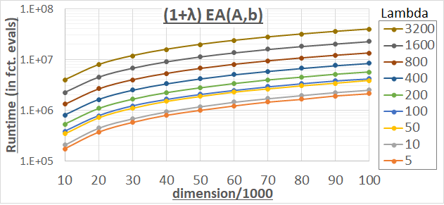
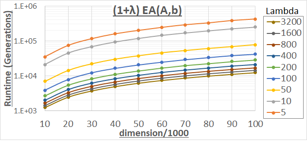
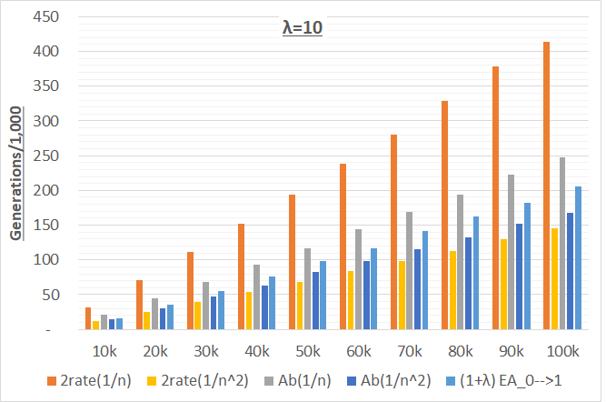
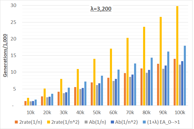
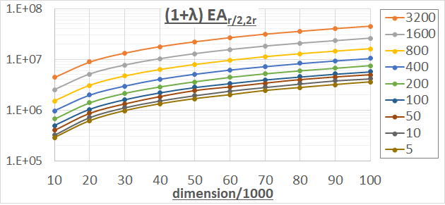
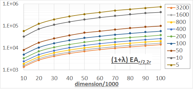
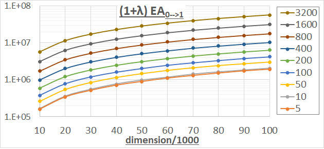
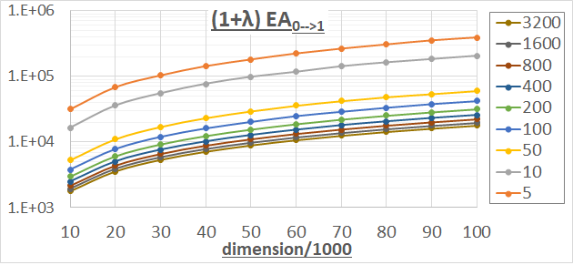
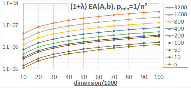
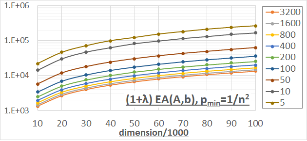
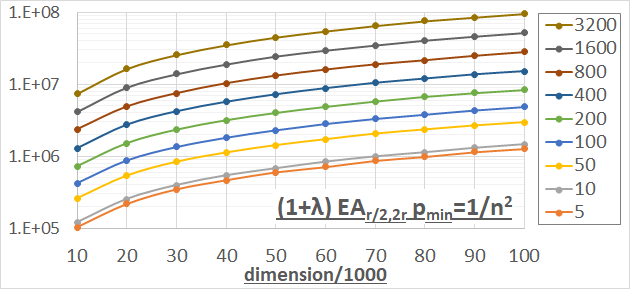
In a first step, we analyze how each algorithm performs across different problem dimensions. To this end, we compute the average optimization time (i.e., the number of function evaluations needed to find an optimal solution) of each of the algorithms described in Section 2 for 100 independent runs. In Figure 1 we show these values for the algorithm $(1+\lambda)$ EA$(A,b)$, for different values of $\lambda$. We also show the average parallel optimization time, measured by the number of generations needed to find an optimal solution, for the $(1+\lambda)$ EA$(A,b)$ in Figure 2. The parallel optimization time equals the average optimization time divided by the offspring population size $\lambda$. This performance measure is useful when the fitness evaluations within one generation are made in parallel.

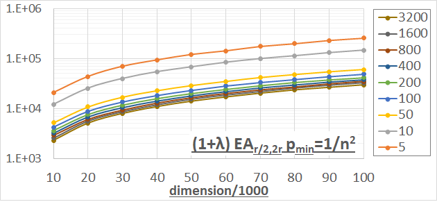
We note without details that the plots for the 2-rate $(1+\lambda)$ EA_r/2,2r and $(1+\lambda)$ EA_0→1 look very similar, but with different values. The relative standard deviation is small for all algorithms: it starts at about 10-15% for $\lambda=5$ and decreases to just 0.5-1.5% for $\lambda=3200$, so we can draw significant conclusions from the average optimization time and the average parallel optimization time plots. Exact figures and standard deviations are available in the appendix.

As expected, we see that for each algorithm and each dimension the average optimization times strictly increase with increasing $\lambda$. Therefore, small values of $\lambda$ are optimal in terms of optimization time. However, in terms of parallel optimization time, the situation is reversed: the algorithms with larger population sizes $\lambda$ require fewer iterations to find the optimum. Therefore, both small and large values of $\lambda$ are worth being used under different circumstances.

4 The Impact of the Lower Bound

One of the key advantages of sampling the mutation rates from the distribution $\operatorname{Bin}_{0\rightarrow 1}(n,p)$ is that it allows to transition from a classical $(1+\lambda)$ EA to a $(1+\lambda)$ variant of RLS that creates each offspring by flipping exactly one uniformly chosen bit. This transition is achieved by reducing $p$ beyond $1/n$, see [CD18a] for a discussion. In the algorithms studied above, we had enforced a lower bound of $1/n$ for $p$. We now relax this lower bound and only require that $p\geq 1/n^{2}$. We study the impact of this relaxed lower bound on the performance of the $(1+\lambda)$ EA$(A,b)$ and the 2-rate $(1+\lambda)$ EA_r/2,2r algorithm. The algorithms with these relaxed lower bounds are denoted by $(1+\lambda)$ EA$(A,b,1/n^{2})$ and 2-rate $(1+\lambda)$ EA${}_{r/2,2r}(1/n^{2})$, respectively.

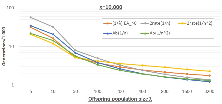
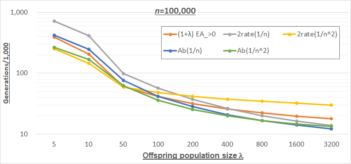
In Figures 3a and 3b we show the average parallel optimization times of the different algorithms for $n=10{,}000$ and $n=100{,}000$, respectively. Recall that the average parallel optimization time equals the average number of generations. Note also that we use a logarithmic scale, to ease the comparison. Note that the standard deviation is still relatively small for the algorithms using $p_{\min}=1/n^{2}$ as well. The only difference is that for 2-rate $(1+\lambda)$ EA${}_{r/2,2r}(1/n^{2})$ it does not decrease with increasing $\lambda$ and is always around 5-10%.

The picture for $n=10{,}000$ is quite similar to that for $n=100{,}000$, and, in fact, for all tested dimensions. To demonstrate this, we plot in Figures 4a and 4b the average parallel optimization times for fixed $\lambda=10$ and $\lambda=3,200$, respectively, which confirm a stable ranking of the different algorithms. We use the parallel optimization time again as performance measure, to ease the comparison with Figures 3a and 3b.

From Figures 3a and 3b we can derive threshold values for $\lambda$ at which the ranking of the algorithms changes.

• For $5\leq\lambda\leq\lambda_{1}$ with $\lambda_{1}$ being a threshold value between 50 and 100, the 2-rate $(1+\lambda)$ EA${}_{r/2,2r}(1/n^{2})$ performs best.

• For $\lambda_{1}\leq\lambda\leq\lambda_{2}$ with $400\leq\lambda_{2}<800$ the $(1+\lambda)$ EA$(A,b,1/n^{2})$ shows best performance.

• For $\lambda_{2}\leq\lambda\leq 3,200$ the $(1+\lambda)$ EA$(A,b)$ minimizes the expected optimization time.

We see that the ranking of algorithms strongly depends on the population size $\lambda$. For small values of $\lambda,$ the 2-rate $(1+\lambda)$ EA${}_{r/2,2r}(1/n^{2})$ performs the best, while for medium values the $(1+\lambda)$ EA$(A,b,1/n^{2})$ wins, and then for large values of $\lambda$ the $(1+\lambda)$ EA$(A,b)$ is superior. Interestingly, for $\lambda=50$, the $(1+\lambda)$ EA_0→1, which uses a static mutation rate, performs on par with the best self-adjusting algorithm.

Generally, for both self-adjusting algorithms, it is more preferable to use $1/n^{2}$ as lower bound for the mutation probability when the population size is small, while for large population sizes a lower bound of $1/n$ seems to work better. For the 2-rate $(1+\lambda)$ EA_r/2,2r, the transition population size is some value $\lambda_{3}$ satisfying $100\leq\lambda_{3}<200$, while for the $(1+\lambda)$ EA$(A,b)$ it is some $\lambda_{2}$ with $400\leq\lambda_{2}<800$. At the same time, while the performance of the 2-rate $(1+\lambda)$ EA_r/2,2r and the 2-rate $(1+\lambda)$ EA${}_{r/2,2r}(1/n^{2})$ drastically depends on the population size and the mutation probability lower bound, the $(1+\lambda)$ EA$(A,b,1/n^{2})$ is more stable and performs rather good for all considered population sizes. Note that the $(1+\lambda)$ EA$(A,b,1/n^{2})$ is the only self-adjusting algorithm which is never significantly worse than the baseline $(1+\lambda)$ EA.

5 Fixed-Budget Performance

Figure 5: Evolution of the average function value over 100 independent runs of different $(1+10)$ EA variants on the $10{,}000$-dimensional OneMax problem, in dependence of the generation. The small plot in the lower right corner zooms into the region in which all algorithms have found function values $\geq 9,900$.

(a)

(b)

Figure 6: Evolution of the average function value over 100 independent runs of different $(1+400)$ EA (a) and $(1+1600)$ EA (b) variants on the $10{,}000$-dimensional OneMax problem, in dependence of the generation.

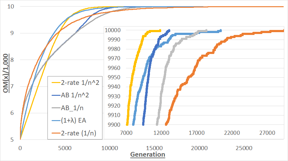
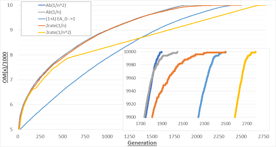
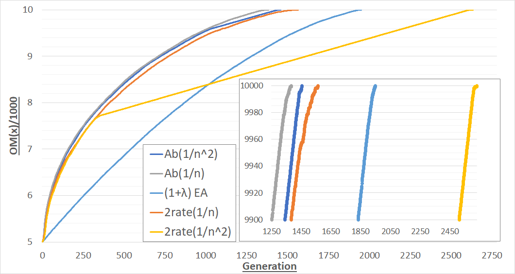
In the sections above, we have only regarded the average optimization times. This measure, albeit very commonly used in the runtime analysis community, does not give any information about how the algorithms perform in an anytime sense. This criticism was addressed in [JZ14, CD18b], where the benefits of fixed-budget and fixed-target analyses are advertised, respectively. We note that, of course, both performance measures have played an important role in empirical evaluations ever since – the contribution of the mentioned papers is rather to be seen in discussing why these measures provide important insights for theoreticians. Figures 5, 6a, 6b show anytime performance plots for selected $(1+10)$ EAs, $(1+400)$ EAs, and $(1+1600)$ EAs, respectively, on the $n=10{,}000$-dimensional OneMax instance.

We see that for $\lambda=10$ (Figure 5) the algorithms demonstrate quite different performance over time, while for larger values of $\lambda$ (Figures 6a, 6b) the performance of the most efficient algorithms seems to be rather stable.

More precisely, the situation is as follows. For generational budgets (note that the budget in terms of fitness evaluations is simply $\lambda$ times larger than the generational budget, since we are dealing with constant offspring population sizes in this paper) up to around 2,590 the 2-rate $(1+\lambda)$ EA_r/2,2r is the most efficient algorithm; then from 2,950 to 5,615 generations $(1+\lambda)$ EA_0→1 is the best one, then the 2-rate $(1+\lambda)$ EA${}_{r/2,2r}(1/n^{2})$, which remains to be the best performing algorithm for all budgets up to 11,800, at which point it hits the optimum. The runner-up is the $(1+\lambda)$ EA$(A,b,1/n^{2})$, third the $(1+\lambda)$ EA$(A,b)$, then the $(1+\lambda)$ EA_0→1 and the worst among the five algorithms is the 2-rate $(1+\lambda)$ EA_r/2,2r (with lower bound $p_{\min}=1/n$). Therefore, for small population sizes, the ranking of the algorithms depends on the budget.

For $\lambda=400$ and $\lambda=1{,}600$, we see that for all budgets the two algorithms $(1+\lambda)$ EA$(A,b,1/n^{2})$ and $(1+\lambda)$ EA$(A,b)$ show similar performance, and are the best among the five algorithms. For $\lambda=400$ the 2-rate $(1+\lambda)$ EA_r/2,2r shows fine performance for budgets up to around 1,700, at which point its performance deteriorates (due to too many offspring sampled with four times the in this case optimal mutation rate). For $\lambda=1{,}600$ this effect disappears, and the 2-rate $(1+\lambda)$ EA_r/2,2r shows fine performance. The performance of the 2-rate $(1+\lambda)$ EA${}_{r/2,2r}(1/n^{2})$ is seen to be the worst of all algorithms for budgets greater than $1{,}400$ for $\lambda=400$ and budgets larger than $1{,}000$ for $\lambda=1{,}600$.

6 2-Rate vs. 3-Rate Adaptation

We next analyze an idea previously communicated in [DGWY19], a 3-rate success-based variant of 2-rate $(1+\lambda)$ EA_r/2,2r, which we call the 3-rate $(1+\lambda)$ EA_r/2,r,2r. This algorithm creates one third of the offspring with mutation rate $c_{1}r/n$, $r/n$, and $c_{2}r/n$, respectively, where $0<c_{1}<1$ and $1<c_{2}$ are hyper-parameters set by the user. The detailed description of the 3-rate $(1+\lambda)$ EA_r/2,r,2r is given in Algorithm 4. In the original work [DGWY19] a similar 3-rate variant has been studied. However, there is no pseudocode of this variant, so it is hard to compare the update rule used in the original work and the one we use.

Following [DGWY19], we use the standard bit mutation operator for all algorithms in this section. It inverts each bit of a string equiprobably with the corresponding mutation rate. So, in contrast to the shift mutation operator used above, it may happen that no bits are flipped in the mutation phase. However, for moderately large $\lambda$, the shift mutation operator performs only slightly better than the standard one (this empirical observation is also confirmed by the findings made in [DYvR⁺18] for the resampling strategy, and can be confirmed theoretically; see the full version of [CD18a] for a similar theoretical justification in the context of the $(1+\lambda)$ EA with static mutation rates), so we believe that the key observations made in this section do not depend on the choice of the mutation operator.

1Initialization: Sample $x\in\{0,1\}^{n}$ u.a.r. and evaluate $f(x)$;

2 Initialize $r\leftarrow r^{\text{init}}$; // We use $r^{\text{init}}=2$;

3 Initialize $c_{1}\geq 1,0<c_{2}<1$; // We use $c_{1}=0.7,c_{2}=1.4$;

4 Optimization: for $t=1,2,3,\ldots$ do

5       for $i=1,\ldots,\lfloor\lambda/3\rfloor$ do

6             Sample $\ell^{(i)}$ from $\operatorname{Bin}(n,c_{1}r/n)$, create $y^{(i)}\leftarrow\operatorname{flip}_{\ell^{(i)}}(x)$, and evaluate $f(y^{(i)})$;

7            

8      for $i=\lfloor\lambda/3\rfloor+1,\ldots,\lfloor 2\lambda/3\rfloor$ do

9             Sample $\ell^{(i)}$ from $\operatorname{Bin}(n,r/n)$, create $y^{(i)}\leftarrow\operatorname{flip}_{\ell^{(i)}}(x)$, and evaluate $f(y^{(i)})$;

10            

11      for $i=\lfloor 2\lambda/3\rfloor+1,\ldots,\lambda$ do

12             Sample $\ell^{(i)}$ from $\operatorname{Bin}(n,c_{2}r/n)$, create $y^{(i)}\leftarrow\operatorname{flip}_{\ell^{(i)}}(x)$, and evaluate $f(y^{(i)})$;

13            

14      $x^{*}\leftarrow\arg\max\{f(y^{(1)}),\ldots,f(y^{(\lambda)})\}$ (ties broken u.a.r.);

15       if $f(x^{*})\geq f(x)$ then $x\leftarrow x^{*}$;

16       Perform one of the following two actions with prob. $1/2:$

• replace $r$ with the mutation rate that $x^{*}$ has been created with;

• replace $r$ with either $c_{1}r$ or $c_{2}r$ equiprobably.

$r\leftarrow\min\{\max\{2,r\},n/4\}$;

17      

Algorithm 4 The 3-rate $(1+\lambda)$ EA${}_{c_{1}r,r,c_{2}r}$ with adaptive mutation rates and three subpopulations

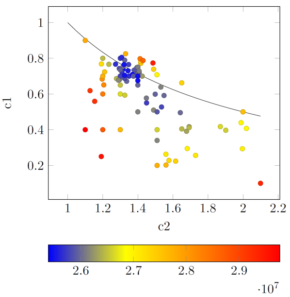
As we have seen in the previous sections, the 2-rate $(1+\lambda)$ EA_r/2,2r performs worse than the $(1+\lambda)$ EA$(A,b)$ for large population sizes. To ensure that this is not caused by a poor tuning of the 2-rate $(1+\lambda)$ EA_r/2,2r, we consider the 3-rate $(1+\lambda)$ EA${}_{c_{1}r,r,c_{2}r}$ on $\lambda=1{,}600$ and check 100 different configurations of $(c_{1},c_{2})$ hyper-parameters for this version. The tuning procedure and its results are illustrated in Figure 7. First, some random values for $c_{1}$ and $c_{2}$ were taken. Then we investigated the areas around values which gave better performance. These results indicated that the best configuration are close to $(c_{1}=0.7,c_{2}=1.4)$. It is also worth mentioning that the performance of the 3-rate $(1+\lambda)$ EA${}_{c_{1}r,r,c_{2}r}$ obtained with the different hyper-parameters differs by up to around 16%. The relative standard deviation of the tested algorithms is about 1%.

Note that we also plot in Figure 7 the line for which $c_{1}=1/c_{2}$, because such a functional dependence was used in [DGWY19]. According to the results of our procedure, the corresponding line does not fit the whole area of good configurations, albeit it does seem to cross some of the best configurations.

Figure 7: Average number of fitness evaluations (shown as color scale) for different hyper-parameters $c_{1},c_{2}$ in 3-rate $(1+\lambda)$ EA${}_{c_{1}r,r,c_{2}r}$ for $\lambda=1{,}600$, $n=100{,}000$.

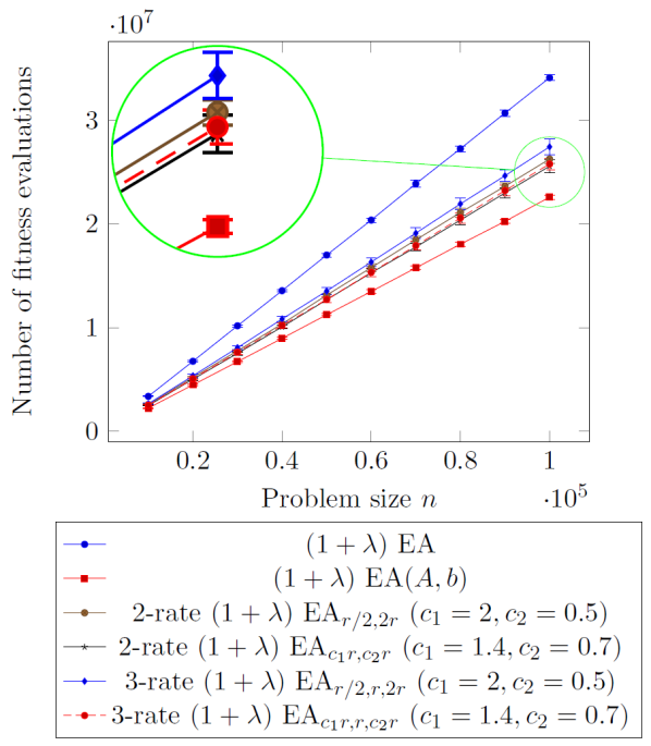
In Figure 8 we plot the performance of the 2-rate $(1+\lambda)$ EA${}_{c_{1}r,c_{2}r}$ and the 3-rate $(1+\lambda)$ EA${}_{c_{1}r,r,c_{2}r}$ using the original hyper-parameters $(c_{1}=2,c_{2}=0.5)$ and using $(c_{1}=1.4,c_{2}=0.7)$. We compare these results to that of the $(1+\lambda)$ EA and the $(1+\lambda)$ EA$(A,b)$ for the population size $\lambda=1{,}600$. For the $(1+\lambda)$ EA and the $(1+\lambda)$ EA$(A,b)$ the relative standard deviation is around 1%, while for the 2-rate $(1+\lambda)$ EA${}_{c_{1}r,c_{2}r}$ and the 3-rate $(1+\lambda)$ EA${}_{c_{1}r,r,c_{2}r}$ it is around 2.5%.

Figure 8 shows that with the original hyper-parameters the 3-rate $(1+\lambda)$ EA_r/2,r,2r performs worse than the 2-rate $(1+\lambda)$ EA_r/2,2r, while with $c_{1}=1.4,c_{2}=0.7$ they both perform better and very similar to each other. However, the algorithms are still outperformed by the $(1+\lambda)$ EA$(A,b)$. Therefore, the careful tuning of the hyper-parameters does not influence the performance of the 2-rate $(1+\lambda)$ EA${}_{c_{1}r,c_{2}r}$ and the 3-rate $(1+\lambda)$ EA${}_{c_{1}r,r,c_{2}r}$ drastically compared to the standard choice of $(c_{1}=0.5,c_{2}=2)$, which confirms the observations made in [DGWY19], where three values of $c2=2.0,1.5,1.2$ with a corresponding $c_{1}=1/c_{2}$ were tested.

Figure 8: Average number of fitness evaluations and its standard deviation for the 2-rate $(1+\lambda)$ EA_r/2,2r and the 3-rate $(1+\lambda)$ EA${}_{c_{1}r,r,c_{2}r}$ with different multipliers compared to the $(1+\lambda)$ EA and the $(1+\lambda)$ EA$(A,b)$ for $\lambda=1{,}600$.

7 Conclusions

We have seen in this work that the ranking of different self-adjusting $(1+\lambda)$ EA variants strongly depends on the population size. Both small population sizes and large ones are of interest, as the former provide the best performance in terms of number of fitness evaluations, while the latter are more efficient in terms of generation number, which is useful when calculating fitness in parallel.

Based on our results, the following conclusions for the OneMax benchmark problem may be drawn: for small offspring population sizes $5\leq\lambda\leq\lambda_{1}$, $\lambda_{1}$ satisfying $50\leq\lambda_{1}<100$ the 2-rate $(1+\lambda)$ EA${}_{r/2,2r}(1/n^{2})$ is the most efficient among the tested algorithms, while for medium population sizes $\lambda_{1}\leq\lambda\leq\lambda_{2}$ with $400\leq\lambda_{2}<800$ the $(1+\lambda)$ EA$(A,b,1/n^{2})$ performs best, and for large offspring population sizes $\lambda_{2}\leq\lambda\leq 3,200$ the $(1+\lambda)$ EA$(A,b)$ with $p_{\min}=1/n$ as the lower bound for the mutation probability should be used. Furthermore, if the evaluation budget is limited and the population size is small, one should pick the algorithms very carefully, as the ranking strongly depends on the budget in this case.

We also confirmed that although a careful selection of the hyper-parameters can improve the performance of the 2-rate $(1+\lambda)$ EA_r/2,2r and the 3-rate $(1+\lambda)$ EA_r/2,r,2r, the default parameters seem to be quite suitably chosen, so that the overall gain of such hyper-parameter tuning seems to be moderate at best. We plan on extending our studies by investigating if similar conclusions can be drawn for the $(1+\lambda)$ EA$(A,b)$ with different values of $A$ and $b$. The results in [DW18] suggest a rather flat dependence of performance on these hyper-parameters for the $(1+1)$ EA, but note that we have considered in our work much larger dimensions and offspring population sizes, so that it is a priori not clear if a similar conclusion holds. We recall from [Len18] that small changes in the parameter setting of an EA can result in drastic performance differences.

As mentioned in the main part, the consistent ranking of the algorithms makes us feel confident about an extension of our work to a rigorous theoretical running time analysis. Such results would offer more detailed insights into the working principles underlying the diverse rankings, and may help to identify the cut-off points where performances of two algorithms intersect.

In another important line of research we plan on investigating whether our conclusions for the OneMax problem can be extended to other, more challenging benchmark problems. A promising direction of such extensions is offered by the W-model [WW18], which allows one to calibrate different features of the optimization problem, such as its ruggedness, the fraction of effective and “dummy” variables, the epistasis, neutrality, separability, etc.

Acknowledgments

Arina Buzdalova was supported by the Government of Russian Federation (Grant 08-08). Carola Doerr was supported by a public grant as part of the Investissement d’avenir project, reference ANR-11-LABX-0056-LMH, and by the Paris Ile-de-France Region. We also acknowledge support from COST Action CA15140 ’Improving Applicability of Nature-Inspired Optimisation by Joining Theory and Practice (ImAppNIO)’ supported by the European Cooperation in Science and Technology.

Appendix A Average Optimization Times and Number of Generations

Figure 9: Average optimization times for 100 independent runs of the 2-rate $(1+\lambda)$ EA_r/2,2r for different values and $5\leq\lambda\leq 3,200$ and different problem dimensions $10k\leq n\leq 100k$.

Figure 10: Average number of generations for 100 independent runs of the 2-rate $(1+\lambda)$ EA_r/2,2r for different values $5\leq\lambda\leq 3,200$ and different problem dimensions $10k\leq n\leq 100k$.

Figure 11: Average optimization times for 100 independent runs of the $(1+\lambda)$ EA_0→1 for different values $5\leq\lambda\leq 3,200$ and different problem dimensions $10k\leq n\leq 100k$, normalized by $n\ln n$.

Figure 12: Average number of generations for 100 independent runs of the $(1+\lambda)$ EA_0→1 for different values $5\leq\lambda\leq 3,200$ and different problem dimensions $10k\leq n\leq 100k$, normalized by $n\ln n$.

Figure 13: Average optimization times for 100 independent runs of the $(1+\lambda)$ EA$(A,b,1/n^{2})$ for different values $5\leq\lambda\leq 3,200$ and different problem dimensions $10k\leq n\leq 100k$.

Figure 14: Average number of generations for 100 independent runs of the $(1+\lambda)$ EA$(A,b,1/n^{2})$ for different values $5\leq\lambda\leq 3,200$ and different problem dimensions $10k\leq n\leq 100k$.

Figure 15: Average optimization times for 100 independent runs of the 2-rate $(1+\lambda)$ EA${}_{r/2,2r}(1/n^{2})$ for different values $5\leq\lambda\leq 3,200$ and different problem dimensions $10k\leq n\leq 100k$.

Figure 16: Average number of generations for 100 independent runs of the 2-rate $(1+\lambda)$ EA${}_{r/2,2r}(1/n^{2})$ for different values $5\leq\lambda\leq 3,200$ and different problem dimensions $10k\leq n\leq 100k$.

$n$	$\lambda$	$(1+\lambda)$ EA0→1		2-rate $(1/n)$		Ab $(1/n)$		2-rate $(1/n^{2})$		Ab $(1/n^{2})$
		avg.	r.dev.	avg.	r.dev.	avg.	r.dev.	avg.	r.dev.	avg.	r.dev.
10,000	1	147,008	14.8%	177,568	14.8%	148,182	14.1%	90,459	13.0%	91,563	15.6%
	5	31,738	17.5%	56,940	17.3%	34,514	13.0%	20,657	13.0%	21,999	13.6%
	10	16,373	13.1%	32,054	15.3%	20,662	9.2%	12,036	11.1%	14,252	7.9%
	50	5,254	7.5%	8,029	12.9%	6,855	6.7%	5,198	8.7%	5,740	3.7%
	100	3,790	4.6%	4,922	9.4%	3,824	5.8%	4,211	9.7%	3,360	4.0%
	200	2,955	3.6%	3,323	8.2%	2,647	3.7%	3,603	10.5%	2,447	2.8%
	400	2,486	2.1%	2,420	5.7%	2,001	2.4%	3,227	11.8%	1,943	1.8%
	800	2,164	1.1%	1,903	3.8%	1,633	1.8%	2,932	13.8%	1,639	1.3%
	1,600	1,945	0.8%	1,582	2.1%	1,393	1.2%	2,576	11.1%	1,450	0.8%
	3,200	1,776	0.6%	1,379	1.8%	1,227	0.8%	2,305	12.3%	1,323	0.8%
20,000	1	311,947	12.6%	399,856	15.1%	318,741	14.6%	195,946	11.7%	192,649	12.8%
	5	68,654	14.3%	122,178	15.7%	73,448	13.8%	43,440	9.4%	46,216	10.1%
	10	35,726	11.1%	71,314	11.0%	44,458	10.1%	25,398	10.1%	30,310	8.4%
	50	10,989	8.0%	17,278	10.5%	14,178	5.8%	10,728	6.7%	11,840	4.5%
	100	7,803	5.4%	10,324	9.6%	7,765	5.8%	8,737	7.3%	6,890	3.7%
	200	6,052	3.5%	6,923	7.9%	5,381	4.0%	7,554	9.8%	4,978	3.1%
	400	5,044	2.1%	4,924	4.5%	4,054	2.8%	6,827	11.3%	3,924	1.9%
	800	4,375	1.5%	3,837	3.6%	3,286	1.6%	6,093	9.1%	3,304	1.2%
	1,600	3,921	0.9%	3,203	2.3%	2,791	1.1%	5,625	10.8%	2,913	0.9%
	3,200	3,574	0.5%	2,762	1.6%	2,448	0.5%	5,112	11.8%	2,650	0.6%
30,000	1	487,226	10.6%	630,449	17.1%	503,393	12.7%	304,196	11.1%	310,610	13.3%
	5	103,709	10.3%	192,890	14.6%	114,129	13.1%	69,405	10.8%	71,197	9.0%
	10	54,922	12.6%	111,448	14.0%	67,800	8.6%	39,620	8.9%	47,255	6.9%
	50	16,963	7.5%	26,418	10.5%	21,820	6.9%	16,738	7.6%	17,956	4.0%
	100	11,987	4.9%	16,021	8.9%	12,149	6.2%	13,445	6.7%	10,397	4.2%
	200	9,200	3.7%	10,656	7.9%	8,180	4.3%	11,681	7.8%	7,477	2.7%
	400	7,617	2.3%	7,438	4.2%	6,152	3.0%	10,475	8.8%	5,882	1.8%
	800	6,588	1.2%	5,844	3.2%	4,957	1.8%	9,345	8.5%	4,967	1.2%
	1,600	5,885	0.7%	4,823	2.0%	4,190	1.1%	8,643	12.8%	4,377	0.7%
	3,200	5,371	0.5%	4,142	1.4%	3,675	0.7%	7,978	11.7%	3,981	0.6%

Table 1: Raw Data for Plots in Section A. Number of generations averaged by 100 runs and its standard deviation for $(1+\lambda)$ EA_0→1, 2-rate $(1+\lambda)$ EA_r/2,2r, $(1+\lambda)$ EA$(A,b)$, 2-rate $(1+\lambda)$ EA${}_{r/2,2r}(1/n^{2})$, $(1+\lambda)$ EA$(A,b,1/n^{2})$. Shift mutation operator is used in all algorithms, avg.=average, r.dev.=relative standard deviation.

$n$	$\lambda$	$(1+\lambda)$ EA0→1		2-rate $(1/n)$		Ab $(1/n)$		2-rate $(1/n^{2})$		Ab $(1/n^{2})$
		avg.	r.dev.	avg.	r.dev.	avg.	r.dev.	avg.	r.dev.	avg.	r.dev.
40,000	1	679,092	11.9%	856,856	13.3%	674,918	11.3%	411,103	11.4%	426,463	13.0%
	5	143,475	11.7%	263,636	13.1%	157,485	12.1%	93,090	9.7%	99,060	9.8%
	10	76,673	10.2%	152,044	13.9%	92,633	9.9%	54,117	8.6%	63,068	7.4%
	50	23,156	7.0%	36,693	10.0%	29,685	7.2%	22,507	6.2%	24,223	4.6%
	100	16,120	5.6%	21,882	9.9%	16,271	6.2%	18,133	7.1%	14,026	4.4%
	200	12,361	3.3%	14,266	7.4%	11,013	4.4%	15,807	7.0%	10,017	2.4%
	400	10,194	2.0%	10,159	5.4%	8,223	2.9%	14,167	8.3%	7,889	1.4%
	800	8,828	1.3%	7,824	3.0%	6,613	1.5%	12,866	7.0%	6,623	0.8%
	1,600	7,864	0.6%	6,427	1.9%	5,598	1.0%	11,816	9.3%	5,842	0.7%
	3,200	7,163	0.4%	5,541	1.3%	4,899	0.5%	10,924	9.3%	5,314	0.5%
50,000	1	870,823	12.9%	1,080,753	12.4%	865,991	12.5%	528,788	14.9%	538,208	12.8%
	5	180,681	11.8%	334,544	14.2%	197,643	11.3%	119,915	10.5%	122,380	9.2%
	10	98,015	11.2%	193,599	12.5%	117,237	9.1%	67,660	7.4%	82,358	8.8%
	50	29,364	7.7%	48,270	11.3%	37,081	6.1%	28,502	5.3%	30,381	4.1%
	100	20,257	4.7%	27,971	9.8%	20,400	5.6%	23,060	7.1%	17,507	3.1%
	200	15,515	2.8%	18,045	6.8%	13,735	3.9%	19,971	8.2%	12,590	2.4%
	400	12,774	2.0%	12,798	4.9%	10,306	2.4%	17,991	9.0%	9,932	1.8%
	800	11,033	1.2%	9,832	3.6%	8,294	1.8%	16,457	10.3%	8,320	1.1%
	1,600	9,835	0.7%	8,093	2.0%	7,021	1.0%	15,261	8.9%	7,315	0.7%
	3,200	8,956	0.5%	6,921	1.2%	6,134	0.6%	14,005	9.9%	6,648	0.5%
60,000	1	1,065,939	10.9%	1,321,699	12.9%	1,056,875	11.4%	665,392	12.5%	645,149	10.9%
	5	222,882	11.6%	398,973	10.5%	241,497	11.9%	141,691	9.4%	153,370	9.9%
	10	116,559	10.5%	237,965	13.4%	143,817	9.7%	83,567	11.0%	98,172	8.9%
	50	35,898	8.5%	56,882	11.1%	45,142	6.3%	34,404	6.2%	36,701	4.0%
	100	24,894	4.8%	33,466	7.5%	24,552	4.0%	28,244	6.2%	21,103	3.5%
	200	18,747	3.4%	22,022	7.2%	16,647	3.9%	24,241	6.0%	15,183	2.6%
	400	15,359	2.0%	15,493	4.2%	12,456	2.6%	21,875	8.8%	11,890	1.4%
	800	13,297	1.3%	11,908	3.3%	9,999	1.7%	19,981	7.8%	9,977	0.8%
	1,600	11,828	0.8%	9,731	2.6%	8,426	1.1%	18,467	10.9%	8,788	0.8%
	3,200	10,758	0.4%	8,315	1.3%	7,363	0.7%	17,024	8.5%	7,987	0.5%

Table 2: Raw Data for Plots in Section A. Number of generations averaged by 100 runs and its standard deviation for $(1+\lambda)$ EA_0→1, 2-rate $(1+\lambda)$ EA_r/2,2r, $(1+\lambda)$ EA$(A,b)$, 2-rate $(1+\lambda)$ EA${}_{r/2,2r}(1/n^{2})$, $(1+\lambda)$ EA$(A,b,1/n^{2})$. Shift mutation operator is used in all algorithms, avg.=average, r.dev.=relative standard deviation.

$n$	$\lambda$	$(1+\lambda)$ EA0→1		2-rate $(1/n)$		Ab $(1/n)$		2-rate $(1/n^{2})$		Ab $(1/n^{2})$
		avg.	r.dev.	avg.	r.dev.	avg.	r.dev.	avg.	r.dev.	avg.	r.dev.
70,000	1	1,256,090	11.6%	1,575,525	12.1%	1,257,547	12.8%	763,835	12.4%	765,788	11.7%
	5	263,995	11.8%	484,544	11.8%	287,358	11.2%	173,293	11.6%	181,169	10.7%
	10	141,720	11.9%	280,866	10.5%	168,687	9.8%	98,930	8.4%	115,841	7.6%
	50	42,174	6.9%	67,508	9.7%	52,244	5.5%	41,157	6.2%	42,866	3.8%
	100	29,002	4.6%	39,666	8.4%	28,912	5.0%	33,200	6.3%	24,763	3.6%
	200	22,056	3.5%	25,905	8.6%	19,621	4.0%	28,777	7.6%	17,649	2.1%
	400	18,078	2.4%	18,103	4.4%	14,510	2.7%	25,956	8.9%	13,903	1.6%
	800	15,550	1.3%	14,002	3.3%	11,674	1.8%	23,607	7.1%	11,671	0.9%
	1,600	13,817	0.6%	11,395	1.9%	9,847	1.1%	21,763	9.0%	10,270	0.7%
	3,200	12,579	0.4%	9,736	1.6%	8,596	0.6%	20,283	10.0%	9,319	0.5%
80,000	1	1,464,944	11.9%	1,784,910	11.9%	1,464,315	11.7%	888,194	13.1%	899,089	12.5%
	5	306,038	11.2%	553,383	11.1%	325,414	9.8%	196,852	9.7%	211,511	9.9%
	10	162,877	10.4%	328,819	12.2%	194,256	9.4%	112,892	7.6%	132,056	7.9%
	50	48,433	6.9%	79,050	11.2%	60,104	5.6%	47,120	5.7%	48,995	3.4%
	100	33,455	5.6%	45,309	7.1%	33,345	4.9%	38,013	5.1%	28,374	3.3%
	200	25,319	4.1%	29,699	6.1%	22,312	3.9%	33,475	8.3%	20,308	2.7%
	400	20,620	2.2%	20,785	6.1%	16,598	2.1%	29,709	8.2%	15,909	1.6%
	800	17,790	1.5%	16,014	3.7%	13,375	1.6%	26,935	7.1%	13,330	1.0%
	1,600	15,822	0.7%	13,010	2.1%	11,277	1.2%	25,466	9.1%	11,724	0.6%
	3,200	14,377	0.5%	11,096	1.1%	9,832	0.6%	23,596	9.7%	10,652	0.5%
90,000	1	1,644,769	12.8%	2,014,968	10.4%	1,663,195	10.3%	1,018,903	12.7%	1,008,852	10.4%
	5	351,978	11.8%	634,502	12.7%	380,506	11.4%	228,885	9.8%	239,240	11.3%
	10	182,743	9.6%	379,167	11.8%	223,083	8.5%	130,161	10.8%	151,945	6.8%
	50	54,042	6.7%	89,176	11.0%	67,712	5.4%	53,486	6.7%	55,810	4.1%
	100	37,998	5.9%	51,540	7.9%	37,983	6.6%	43,632	5.9%	31,916	3.5%
	200	28,529	3.7%	33,267	6.2%	25,451	3.8%	37,658	7.6%	22,852	2.7%
	400	23,249	2.0%	23,480	4.4%	18,836	2.9%	33,974	8.0%	17,956	1.6%
	800	20,002	1.2%	17,987	3.2%	15,023	1.6%	31,103	9.3%	15,022	1.0%
	1,600	17,795	0.8%	14,592	1.7%	12,653	0.9%	28,968	9.7%	13,207	0.6%
	3,200	16,153	0.4%	12,506	1.1%	11,064	0.6%	26,533	9.5%	12,006	0.5%

Table 3: Raw Data for Plots in Section A. Number of generations averaged by 100 runs and its standard deviation for $(1+\lambda)$ EA_0→1, 2-rate $(1+\lambda)$ EA_r/2,2r, $(1+\lambda)$ EA$(A,b)$, 2-rate $(1+\lambda)$ EA${}_{r/2,2r}(1/n^{2})$, $(1+\lambda)$ EA$(A,b,1/n^{2})$. Shift mutation operator is used in all algorithms, avg.=average, r.dev.=relative standard deviation.

$n$	$\lambda$	$(1+\lambda)$ EA0→1		2-rate $(1/n)$		Ab $(1/n)$		2-rate $(1/n^{2})$		Ab $(1/n^{2})$
		avg.	r.dev.	avg.	r.dev.	avg.	r.dev.	avg.	r.dev.	avg.	r.dev.
100,000	1	1,873,666	13.4%	2,222,691	10.9%	1,860,718	13.4%	1,143,933	11.7%	1,122,686	10.6%
	5	389,110	10.2%	716,372	13.6%	420,165	10.4%	253,747	11.7%	264,171	8.5%
	10	205,086	12.0%	414,043	10.4%	248,184	9.7%	146,132	8.2%	167,244	7.0%
	50	60,200	6.2%	98,223	8.7%	76,772	5.6%	59,357	5.7%	62,693	3.8%
	100	42,151	5.0%	57,325	6.9%	41,520	4.1%	48,659	6.6%	35,814	4.1%
	200	31,762	3.4%	37,588	6.8%	28,215	3.7%	41,634	4.6%	25,431	2.2%
	400	25,846	2.1%	26,227	5.0%	20,900	2.6%	37,583	8.3%	19,984	1.6%
	800	22,229	1.2%	20,055	3.2%	16,681	1.4%	34,965	9.3%	16,691	0.9%
	1,600	19,744	0.7%	16,325	2.0%	14,112	1.0%	32,494	11.6%	14,691	0.6%
	3,200	17,956	0.4%	13,966	1.1%	12,296	0.6%	29,796	11.1%	13,344	0.5%

Table 4: Raw Data for Plots in Section A. Number of generations averaged by 100 runs and its standard deviation for $(1+\lambda)$ EA_0→1, 2-rate $(1+\lambda)$ EA_r/2,2r, $(1+\lambda)$ EA$(A,b)$, 2-rate $(1+\lambda)$ EA${}_{r/2,2r}(1/n^{2})$, $(1+\lambda)$ EA$(A,b,1/n^{2})$. Shift mutation operator is used in all algorithms, avg.=average, r.dev.=relative standard deviation.

Table 5: Raw Data for Figure 8. Average number of fitness evaluations for 2-rate $(1+\lambda)$ EA_r/2,2r (2-rate) and 3-rate $(1+\lambda)$ EA_r/2,r,2r (3-rate) with different hyper-parameters (0.5, 2 and 0.7, 1.4) compared to $(1+\lambda)$ EA and $(1+\lambda)$ EA$(A,b)$ (Ab) for $\lambda=1600.$ Standard mutation operator is used in all algorithms, avg.=average, r.dev.=relative standard deviation.

$n$	$(1+\lambda)$ EA		2-rate (0.5)		2-rate (0.7)		3-rate (0.5)		3-rate (0.7)		Ab
	avg.	r.dev.	avg.	r.dev.	avg.	r.dev.	avg.	r.dev.	avg.	r.dev.	avg.	r.dev.
10,000	3,362,177	1.0%	2,647,488	2.4%	2,473,264	2.2%	2,645,616	3.1%	2,498,816	2.5%	2,228,449	1.2%
20,000	6,744,593	1.1%	5,378,496	3.2%	5,011,088	2.4%	5,341,728	3.4%	5,056,128	2.5%	4,466,209	1.1%
30,000	10,167,969	1.0%	8,097,168	2.5%	7,512,784	2.5%	8,055,056	2.4%	7,609,648	2.5%	6,703,809	1.1%
40,000	13,556,897	0.9%	10,881,344	2.4%	10,063,600	1.9%	10,825,376	2.1%	10,201,920	2.6%	8,957,105	1.0%
50,000	16,995,265	1.0%	13,659,776	2.8%	12,678,240	2.1%	13,523,152	2.6%	12,706,512	2.2%	11,233,585	1.0%
60,000	20,369,121	1.0%	16,393,136	2.4%	15,283,856	2.4%	16,322,656	2.5%	15,329,392	2.6%	13,482,257	1.1%
70,000	23,874,081	1.4%	19,181,872	2.5%	17,763,856	2.1%	19,106,128	2.8%	17,899,920	2.2%	15,755,281	1.1%
80,000	27,254,449	1.0%	22,074,384	3.0%	20,368,800	2.2%	21,933,152	2.5%	20,575,680	2.4%	18,043,073	1.2%
90,000	30,697,777	1.0%	24,806,320	2.6%	22,990,288	2.1%	24,648,208	2.3%	23,221,920	2.3%	20,245,025	0.9%
100,000	34,105,201	0.8%	27,558,720	2.4%	25,569,168	2.4%	27,436,784	2.7%	25,784,448	2.1%	22,579,393	1.0%

References

- [AD11] Anne Auger and Benjamin Doerr. Theory of Randomized Search Heuristics. World Scientific, 2011.
- [AM16] Aldeida Aleti and Irene Moser. A systematic literature review of adaptive parameter control methods for evolutionary algorithms. ACM Computing Surveys, 49:56:1–56:35, 2016.
- [Bäc92] Thomas Bäck. The interaction of mutation rate, selection, and self-adaptation within a genetic algorithm. In Proc. of Parallel Problem Solving from Nature (PPSN’92), pages 87–96. Elsevier, 1992.
- [Bäc93] Thomas Bäck. Optimal mutation rates in genetic search. In Proc. of the 5th International Conference on Genetic Algorithms (ICGA’93), pages 2–8. Morgan Kaufmann, 1993.
- [BGH+13] Edmund K. Burke, Michel Gendreau, Matthew R. Hyde, Graham Kendall, Gabriela Ochoa, Ender Özcan, and Rong Qu. Hyper-heuristics: a survey of the state of the art. JORS, 64(12):1695–1724, 2013.
- [BLS14] Golnaz Badkobeh, Per Kristian Lehre, and Dirk Sudholt. Unbiased black-box complexity of parallel search. In Proc. of Parallel Problem Solving from Nature (PPSN’14), volume 8672 of Lecture Notes in Computer Science, pages 892–901. Springer, 2014.
- [CD18a] Eduardo Carvalho Pinto and Carola Doerr. A simple proof for the usefulness of crossover in black-box optimization. In Proc. of Parallel Problem Solving from Nature (PPSN’18), volume 11102 of Lecture Notes in Computer Science, pages 29–41. Springer, 2018. Full version available at http://arxiv.org/abs/1812.00493.
- [CD18b] Eduardo Carvalho Pinto and Carola Doerr. Towards a more practice-aware runtime analysis of evolutionary algorithms. CoRR, abs/1812.00493, 2018. An extended abstract appeared in Proc. of Artificial Evolution (EA’17), pages 298–305.
- [DD18a] Benjamin Doerr and Carola Doerr. Optimal static and self-adjusting parameter choices for the genetic algorithm. Algorithmica, 80:1658–1709, 2018.
- [DD18b] Benjamin Doerr and Carola Doerr. Theory of parameter control mechanisms for discrete black-box optimization: Provable performance gains through dynamic parameter choices. In Benjamin Doerr and Frank Neumann, editors, Theory of Randomized Search Heuristics in Discrete Search Spaces. Springer, 2018. To appear. Available online at https://arxiv.org/abs/1804.05650.
- [DDE15] Benjamin Doerr, Carola Doerr, and Franziska Ebel. From black-box complexity to designing new genetic algorithms. Theoretical Computer Science, 567:87–104, 2015.
- [DDL19] Benjamin Doerr, Carola Doerr, and Johannes Lengler. Self-adjusting mutation rates with provably optimal success rules. In Proc. of Genetic and Evolutionary Computation Conference (GECCO’19). ACM, 2019. To appear. Full version available online at http://arxiv.org/abs/1902.02588.
- [DDY16] Benjamin Doerr, Carola Doerr, and Jing Yang. Optimal parameter choices via precise black-box analysis. In Proc. of Genetic and Evolutionary Computation Conference (GECCO’16), pages 1123–1130. ACM, 2016.
- [DGWY19] Benjamin Doerr, Christian Gießen, Carsten Witt, and Jing Yang. The ( $$1+\lambda $$ 1 + ) evolutionary algorithm with self-adjusting mutation rate. Algorithmica, 81(2):593–631, 2019.
- [Doe18] Carola Doerr. Complexity theory for discrete black-box optimization heuristics. CoRR, abs/1801.02037, 2018.
- [DW18] Carola Doerr and Markus Wagner. On the effectiveness of simple success-based parameter selection mechanisms for two classical discrete black-box optimization benchmark problems. In Proc. of Genetic and Evolutionary Computation Conference (GECCO’18), pages 943–950. ACM, 2018.
- [DYvR+18] Carola Doerr, Furong Ye, Sander van Rijn, Hao Wang, and Thomas Bäck. Towards a theory-guided benchmarking suite for discrete black-box optimization heuristics: Profiling (1 + ) EA variants on onemax and leadingones. In Proc. of Genetic and Evolutionary Computation Conference (GECCO’18), pages 951–958. ACM, 2018.
- [EHM99] Agoston Endre Eiben, Robert Hinterding, and Zbigniew Michalewicz. Parameter control in evolutionary algorithms. IEEE Transactions on Evolutionary Computation, 3:124–141, 1999.
- [FCSS08] Álvaro Fialho, Luís Da Costa, Marc Schoenauer, and Michèle Sebag. Extreme value based adaptive operator selection. In Proc. of Parallel Problem Solving from Nature (PPSN’08), volume 5199 of Lecture Notes in Computer Science, pages 175–184. Springer, 2008.
- [FCSS10] Álvaro Fialho, Luís Da Costa, Marc Schoenauer, and Michèle Sebag. Analyzing bandit-based adaptive operator selection mechanisms. Annals of Mathematics and Artificial Intelligence, 60:25–64, 2010.
- [Jan13] Thomas Jansen. Analyzing Evolutionary Algorithms—The Computer Science Perspective. Springer, 2013.
- [JDJW05] Thomas Jansen, Kenneth A. De Jong, and Ingo Wegener. On the choice of the offspring population size in evolutionary algorithms. Evolutionary Computation, 13:413–440, 2005.
- [JZ14] Thomas Jansen and Christine Zarges. Performance analysis of randomised search heuristics operating with a fixed budget. Theoretical Computer Science, 545:39–58, 2014.
- [KHE15] Giorgos Karafotias, Mark Hoogendoorn, and A.E. Eiben. Parameter control in evolutionary algorithms: Trends and challenges. IEEE Transactions on Evolutionary Computation, 19:167–187, 2015.
- [KMH+04] Stefan Kern, Sibylle D. Müller, Nikolaus Hansen, Dirk Büche, Jiri Ocenasek, and Petros Koumoutsakos. Learning probability distributions in continuous evolutionary algorithms - a comparative review. Natural Computing, 3:77–112, 2004.
- [Len18] Johannes Lengler. A general dichotomy of evolutionary algorithms on monotone functions. In Proc. of Parallel Problem Solving from Nature (PPSN’18), volume 11102 of Lecture Notes in Computer Science, pages 3–15. Springer, 2018.
- [LS11] Jörg Lässig and Dirk Sudholt. Adaptive population models for offspring populations and parallel evolutionary algorithms. In Proc. of Foundations of Genetic Algorithms (FOGA’11), pages 181–192. ACM, 2011.
- [MLS10] Jorge Maturana, Frédéric Lardeux, and Frédéric Saubion. Autonomous operator management for evolutionary algorithms. Journal of Heuristics, 16:881–909, 2010.
- [Rec73] Ingo Rechenberg. Evolutionsstrategie. Friedrich Fromman Verlag (Günther Holzboog KG), Stuttgart, 1973.
- [Thi09] Dirk Thierens. On benchmark properties for adaptive operator selection. In Proc. of Genetic and Evolutionary Computation Conference (GECCO’09), Companion Material, pages 2217–2218. ACM, 2009.
- [WW18] Thomas Weise and Zijun Wu. Difficult features of combinatorial optimization problems and the tunable w-model benchmark problem for simulating them. In Proc. of Genetic and Evolutionary Computation Conference (GECCO’18), Companion Material), pages 1769–1776. ACM, 2018.