A Systematic Study of Leveraging Subword Information
for Learning Word Representations

Abstract

The use of subword-level information (e.g., characters, character n-grams, morphemes) has become ubiquitous in modern word representation learning. Its importance is attested especially for morphologically rich languages which generate a large number of rare words. Despite a steadily increasing interest in such subword-informed word representations, their systematic comparative analysis across typologically diverse languages and different tasks is still missing. In this work, we deliver such a study focusing on the variation of two crucial components required for subword-level integration into word representation models: 1) segmentation of words into subword units, and 2) subword composition functions to obtain final word representations. We propose a general framework for learning subword-informed word representations that allows for easy experimentation with different segmentation and composition components, also including more advanced techniques based on position embeddings and self-attention. Using the unified framework, we run experiments over a large number of subword-informed word representation configurations (60 in total) on 3 tasks (general and rare word similarity, dependency parsing, fine-grained entity typing) for 5 languages representing 3 language types. Our main results clearly indicate that there is no “one-size-fits-all” configuration, as performance is both language- and task-dependent. We also show that configurations based on unsupervised segmentation (e.g., BPE, Morfessor) are sometimes comparable to or even outperform the ones based on supervised word segmentation.

1 Introduction

Word representations are central to a wide variety of NLP tasks (Collobert et al., 2011; Chen and Manning, 2014; Jia and Liang, 2016; Ammar et al., 2016; Goldberg, 2017; Peters et al., 2018; Kudo, 2018, inter alia). Standard word representation models are based on the distributional hypothesis (Harris, 1954) and induce representations from large unlabeled corpora using word co-occurrence statistics (Mikolov et al., 2013; Pennington et al., 2014; Levy and Goldberg, 2014). However, as pointed out by recent work Bojanowski et al. (2017); Vania and Lopez (2017); Pinter et al. (2017); Chaudhary et al. (2018); Zhao et al. (2018), mapping a finite set of word types into corresponding word representations limits the capacity of these models to learn beyond distributional information, which leads to several fundamental limitations.

The standard approaches ignore the internal structure of words, that is, the syntactic or semantic composition from subwords or morphemes to words, and are incapable of parameter sharing at the level of subword units. Assigning only a single vector to each word causes the data sparsity problem, especially in resource-poor settings where huge amounts of training data cannot be guaranteed. The issue is also prominent for morphologically rich languages (e.g., Finnish) with productive morphological systems that generate a large number of infrequent/rare words Gerz et al. (2018). Although potentially useful information on word relationships is hidden in their internal subword-level structure, subword-agnostic word representation models do not take these structure features into account and are effectively unable to represent rare words accurately, or unseen words at all.

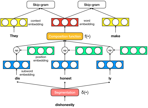
Figure 1: Illustration of the general framework for learning subword-informed word representations, with the focus on two crucial components: 1) segmentation of words and 2) subword embedding composition. By varying the two components, and optionally including or excluding position embeddings from the computations, we obtain a wide spectrum of different subword-informed configurations used in the study (see §2). Our word-level representation model in this work is skip-gram (on the top layer of the figure), but it can be replaced by any other distributional word-level model.

Therefore, there has been a surge of interest in subword-informed word representation architectures aiming to address these gaps. A large number of architectures has been proposed in related research, and they can be clustered over the two main axes Lazaridou et al. (2013); Luong et al. (2013); Qiu et al. (2014); Cotterell and Schütze (2015); Wieting et al. (2016); Avraham and Goldberg (2017); Vania and Lopez (2017); Pinter et al. (2017); Cotterell and Schütze (2018). First, the models differ in the chosen method for segmenting words into subwords. The methods range from fully supervised approaches (Cotterell and Schütze, 2015) to e.g. unsupervised approaches based on BPE (Heinzerling and Strube, 2018). Second, another crucial aspect is the subword composition function used to obtain word embeddings from the embeddings of each word’s constituent subword units. Despite a steadily increasing interest in such subword-informed word representations, their systematic comparative analysis across the two main axes, as well as across typologically diverse languages and different tasks is still missing.

In this work, we conduct a systematic study of a variety of subword-informed word representation architectures that all can be described by a general framework illustrated by Figure 1. The framework enables straightforward experimentation with prominent word segmentation methods (e.g., BPE, Morfessor, supervised segmentation systems) as well as subword composition functions (e.g., addition, self-attention), resulting in a large number of different subword-informed configurations.

Our study aims at providing answers to the following crucial questions: Q1) How generalizable are subword-informed models across typologically diverse languages and across different downstream tasks? Do different languages and tasks require different configurations to reach peak performances or is there a single best-performing configuration? Q2) How important is it to choose an appropriate segmentation and composition method? How effective are more generally applicable unsupervised segmentation methods? Is it always better to resort to a supervised method, if available? Q3) Is there a difference in performance with and without the full word representation? Can more advanced techniques based on position embeddings and self-attention yield better task performance?

We evaluate subword-informed word representation configurations originating from the general framework in three different tasks using standard benchmarks and evaluation protocols: 1) general and rare word similarity and relatedness, 2) dependency parsing, and 3) fine-grained entity typing for 5 languages representing 3 language families (fusional, introflexive, agglutinative). We show that different tasks and languages indeed require diverse subword-informed configurations to reach peak performance: this calls for a more careful language- and task-dependent tuning of configuration components. We also show that more sophisticated configurations are particularly useful for representing rare words, and that unsupervised segmentation methods can be competitive to supervised segmentation in tasks such as parsing or fine-grained entity typing. We hope that this paper will provide useful points of comparison and comprehensive guidance for developing next-generation subword-informed word representation models for typologically diverse languages.

2 Methodology

The general framework for learning subword-informed word representations, illustrated by Figure 1, is introduced in §2.1. We then describe its main components: segmentation of words into subword units (§2.2), subword and position embeddings (§2.3), and subword embedding composition functions (§2.4), along with all the configurations for these components used in our evaluation.

2.1 General Framework

Formally, given a word $w$, its word embedding $\mathbf{w}$ can be computed by the composition of its subword embeddings as follows:

$$\mathbf{w}=f_{\mathbf{\Theta}}(\delta(w),\mathbf{W}_{s},\mathbf{W}_{p}),$$ (1)

where $\delta(w)$ is a deterministic function that segments $w$ into an ordered sequence of its constituent subword units $S_{w}=(s_{w_{i}})_{1}^{n}$, with $s_{w_{i}}\in\mathcal{S}$ being a subword type from the subword vocabulary $\mathcal{S}$ of size $|\mathcal{S}|$. Optionally, some segmentation methods can also generate a sequence of the corresponding morphotactic tags $T_{w}=(t_{w_{i}})_{1}^{n}$. Alone or together with $T_{w}$, $S_{w}$ is embedded into a sequence of subword representations $\mathbf{S}_{w}=(\mathbf{s}_{w_{i}})_{1}^{n}$ from the subword embedding matrix $\mathbf{W}_{s}\in\mathbb{R}^{|\mathcal{S}|\times d}$, where $d$ is the dimensionality of subword embeddings. Another optional step is to obtain a sequence of position embeddings $\mathbf{P}_{w}=(\mathbf{p}_{w_{i}})_{1}^{n}$: they are taken from the position embedding matrix $\mathbf{W}_{p}\in\mathbb{R}^{p\times d}$, where $p$ is the maximum number of the unique positions. $\mathbf{P}_{w}$ can interact with $\mathbf{S}_{w}$ to compute the final representations for subwords $\mathbf{R}_{w}=(\mathbf{r}_{w_{i}})_{1}^{n}$ Vaswani et al. (2017). $f_{\mathbf{\Theta}}$ is a composition function taking $\mathbf{R}_{w}$ as input and outputting a single vector $\mathbf{w}$ as the word embedding of $w$.

For the distributional “word-level” training, similar to prior work Bojanowski et al. (2017), we adopt the standard skip-gram with negative sampling (sgns) Mikolov et al. (2013) with bag-of-words contexts. However, we note that other distributional models can also be used under the same framework. Again, following Bojanowski et al. (2017), we calculate the word embedding $\mathbf{w}_{t}\in\mathbb{R}^{d}$ for each target word $w_{t}$ using the formulation from Eq. (1), and parametrize context words with another word embedding matrix $\mathbf{W}_{c}\in\mathbb{R}^{|\mathcal{V}|\times d}$, where $|\mathcal{V}|$ is the size of word vocabulary $\mathcal{V}$.

2.2 Segmentation of Words into Subwords

We consider three well-known segmentation methods for the function $\delta$, briefly outlined here.

Supervised Morphological Segmentation

We use CHIPMUNK Cotterell et al. (2015) as a representative supervised segmentation system, proven to provide a good trade-off between accuracy and speed. It is based on semi-Markov conditional random fields (Sarawagi and Cohen, 2005). For each word, apart from generating $S_{w}$, it also outputs the corresponding morphotactic tags $T_{w}$. In §2.3 we discuss how to incorporate information from $T_{w}$ into subword representations.

Morfessor

Morfessor Smit et al. (2014) denotes a family of generative probabilistic models for unsupervised morphological segmentation used, among other applications, to learn morphologically-aware word embeddings (Luong et al., 2013).

$\delta$	$\delta$(dishonestly)
CHIPMUNK	(dis, honest, ly)
	(prefix, root, suffix)
Morfessor	(dishonest, ly)
BPE	(dish, on, est, ly)

Table 1: Segmentations of the word dishonestly.

BPE

Byte Pair Encoding (BPE; Gage (1994)) is a simple data compression algorithm. It has become a de facto standard for providing subword information in neural machine translation (Sennrich et al., 2016). The input word is initially split into a sequence of characters, with each unique character denoted as a byte. BPE then iteratively replaces the most common pair of consecutive bytes with a new byte that does not occur within the data, and the number of iterations can be set in advance to control the granularity of the byte combinations.

An example output for all three methods is shown in Table 1. Note that a standard practice in subword-informed models is to also insert the entire word token into $S_{w}$ Bojanowski et al. (2017). This is, however, again an optional step and we evaluate configurations with and without the inclusion of the word token in $S_{w}$.

2.3 Subword and Position Embeddings

The next step is to encode $S_{w}$ (or the tuple ($S_{w}$, $T_{w}$) for CHIPMUNK) to construct a sequence of subword representations $\mathbf{S}_{w}$. Each row of the subword embedding matrix $\mathbf{W}_{s}$ is simply defined as the embedding of a unique subword. For CHIPMUNK, we define each row in $\mathbf{W}_{s}$ as the concatenation of the subword $s$ and its predicted tag $t$. We also test CHIPMUNK configurations without the use of $T_{w}$ to analyze its contribution.

After generating $\mathbf{S}_{w}$, an optional step is to have a learnable position embedding sequence $\mathbf{P}_{w}$ further operate on $\mathbf{S}_{w}$ to encode the order information. Similar to $\mathbf{W}_{s}$, the definition of the position embedding matrix $\mathbf{W}_{p}$ also varies: for Morfessor and BPE, we use the absolute positions of subwords in the sequence $S_{w}$, whereas for CHIPMUNK morphotactic tags are encoded directly as positions.

Finally, following prior work (Gehring et al., 2017; Mikolov et al., 2018), we use addition and element-wise multiplication between each subword vector $\mathbf{s}$ from $\mathbf{S}_{w}$ and the corresponding position vector $\mathbf{p}$ from $\mathbf{P}_{w}$ to compute each entry $\mathbf{r}$ for the final sequence of subword vectors $\mathbf{R}_{w}$:

$$\mathbf{r}=\mathbf{s}+\mathbf{p}\hskip 11.38109pt\textnormal{or}\hskip 11.38109pt\mathbf{r}=\mathbf{s}\odot\mathbf{p}.$$ (2)

2.4 Composition Functions

A composition function $f_{\mathbf{\Theta}}$ is then applied to the sequence of subword embeddings $\mathbf{R}_{w}$ to compute the final word embedding $\mathbf{w}$. We investigate three composition functions: 1) addition, 2) single-head and 3) multi-head self-attention (Vaswani et al., 2017; Lin et al., 2017). Addition is used in the original fastText model of Bojanowski et al. (2017), and remains a strong baseline for many tasks. However, addition treats each subword with the same importance, ignoring semantic composition and interactions among the word’s constituent subwords. Therefore, we propose to use a self-attention mechanism, that is, a learnable weighted addition as the composition function on subword sequences. To the best of our knowledge, we are the first to apply a self-attention mechanism to the problem of subword composition.

Composition Based on Self-Attention

Our self-attention mechanism is inspired by Lin et al. (2017). It is essentially a multilayer feed-forward neural network without bias term, which generates a weight matrix for the variable length input $\mathbf{R}_{w}$:

$$\mathbf{H}_{w}=tanh(\mathbf{W}_{h_{1}}\mathbf{R}_{w}^{T})$$ (3)

$$\mathbf{A}_{w}=softmax(\mathbf{W}_{h_{2}}\mathbf{H}_{w})$$ (4)

Each row of $\mathbf{A}_{w}$ is a weight vector for rows of $\mathbf{R}_{w}$, which models different aspects of semantic compositions and interactions. For the single-head self-attention, $\mathbf{A}_{w}$ degenerates to a row vector as the final attention vector $\mathbf{a}_{w}$. For the multi-head self-attention, we average the rows of $\mathbf{A}_{w}$ to generate $\mathbf{a}_{w}$. Finally, $\mathbf{w}$ is computed as the weighted addition of subword embeddings from $\mathbf{R}_{w}$: $\mathbf{w}=\sum_{w_{1}}^{w_{n}}a_{w_{i}}\mathbf{r}_{w_{i}}$.

3 Experimental Setup

Component	Option	Label
Segmentation	CHIPMUNK	sms
	Morfessor	morf
	BPE	bpe
Morphotactic tag	concatenated with	st
	subword (only sms)
Word token	exclusion	w-
	inclusion	w+
Position embedding	exclusion	p-
	additive	pp
	multiplicative	mp
Composition function	addition	add
	single head attention	att
	multi-head attention	mtx

Table 2: Different components used to construct subword-informed configurations, and their labels.

We train different subword-informed model configurations on 5 languages representing 3 morphological language types: English (en), German (de), Finnish (fi), Turkish (tr) and Hebrew (he), see Table 3. We then evaluate the resulting subword-informed word embeddings in three distinct tasks: 1) general and rare word similarity and relatedness, 2) syntactic parsing, and 3) fine-grained entity typing. The three tasks have been selected in particular as they require different degrees of syntactic and semantic information to be stored in the input word embeddings, ranging from a purely semantic task (word similarity) over a hybrid syntactic-semantic task of entity typing to syntactic parsing.

Subword-Informed Configurations

We train a large number of subword-informed configurations by varying the segmentation method $\delta$ (§2.2), subword embeddings $\mathbf{W}_{s}$, the inclusion of position embeddings $\mathbf{W}_{p}$ and the operations on $\mathbf{W}_{s}$ (§2.3), and the composition functions $f_{\mathbf{\Theta}}$ (§2.4). The configurations are based on the following variations of constituent components: (1) For the segmentation $\delta$, we test a supervised morphological system CHIPMUNK (sms), Morfessor (morf) and BPE (bpe). A word token can be optionally inserted into the subword sequence $S_{w}$ for all three segmentation methods (ww) or left out (w-); (2) We can only embed the subword $s$ for morf and bpe, while with sms we can optionally embed the concatenation of the subword and its morphotactic tag $s:t$ (st); (3) We test subword embedding learning without position embeddings (p-), or we integrate them using addition (pp) or element-wise multiplication (mp); (4) For the composition function function $f_{\mathbf{\Theta}}$, we experiment with addition (add), single head self-attention (att), and multi-head self-attention (mtx). Table 2 provides an overview of all components used to construct a variety of subword-informed configurations used in our evaluation.

The variations of components from Table 2 yield 24 different configurations in total for sms, and 18 for morf and bpe. We use pretrained CHIPMUNK models for all test languages except for Hebrew, as Hebrew lacks gold segmentation data. Following Vania and Lopez (2017), we use the default parameters for Morfessor, and 10k merge operations for BPE across languages. We use available BPE models pre-trained on Wikipedia by Heinzerling and Strube (2018).

Two well-known word representation models, which can also be described by the general framework from Figure 1, are used as insightful baselines: the subword-agnostic sgns model (Mikolov et al., 2013) and fastText (ft) (Bojanowski et al., 2017). ft computes the target word embedding using addition as the composition function, while the segmentation is straightforward: the model simply generates all character n-grams of length 3 to 6 and adds them to $S_{w}$ along with the full word.

Training Setup

Our training data for all languages is Wikipedia. We lowercase all text and replace all digits with a generic tag #. The statistics of the training corpora are provided in Table 3.

All subword-informed variants are trained on the same data and share the same parameters for the sgns model. Further, we use adagrad (Duchi et al., 2011) with a linearly decaying learning rate, and do a grid search of learning rate and batch size for each $\delta$ on the German WordSim-353 data set (ws; Leviant and Reichart (2015)). The hyper-parameters are then fixed for all other languages and evaluation runs. Finally, we set the learning rate to 0.05 for sms and bpe, and 0.075 for morf, and the batch size to 1024 for all the settings.

Typology	Language	#tokens	#types
Fusional	English (en)	600M	900K
	German (de)	200M	940K
Agglutinative	Finnish (fi)	66M	600K
	Turkish (tr)	52M	300K
Introflexive	Hebrew (he)	90M	410K

Table 3: Statistics of our Wikipedia training corpora. For faster training, we use one third of the entire Wikipedia corpus for en and de.

3.1 Evaluation Tasks

Word Similarity and Relatedness

These standard intrinsic evaluation tasks test the semantics of word representations (Pennington et al., 2014; Bojanowski et al., 2017). The evaluations are performed using the Spearman’s rank correlation score between the average of human judgement similarity scores for word pairs and the cosine similarity between two word embeddings constituting each word pair. We use Multilingual SimLex-999 (simlex; Hill et al. (2015); Leviant and Reichart (2015); Mrkšić et al. (2017)) for English, German and Hebrew, each containing 999 word pairs annotated for true semantic similarity. We further evaluate embeddings on FinnSim-300 (fs300) produced by Venekoski and Vankka (2017) for Finnish and AnlamVer (an; Ercan and Yıldız (2018)) for Turkish. We also run experiments on the WordSim-353 test set (ws; Finkelstein et al. (2002)), and its portions oriented towards true similarity (ws-sim) and broader relatedness (ws-rel) portion for English and German.

		Best	2nd Best	Worst	sgns	ft
en	ws	.656 (sms.w-.st.att)	.655 (sms.w-.pp.att)	.440 (bpe.w-.mp.mtx)	.634	.643
	ws-sim	.708 (sms.ww.st.mtx)	.707 (sms.w-.st.att)	.475 (bpe.w-.mp.att)	.702	.706
	ws-rel	.625 (sms.w-.p-.add)	.620 (sms.w-.st.att)	.438 (bpe.w-.mp.mtx)	.579	.586
	simlex	.283 (sms.ww.p-.add)	.282 (morf.w-.p-.add)	.182 (bpe.w-.mp.add)	.300	.307
de	ws	.633 (sms.ww.pp.add)	.633 (sms.ww.p-.add)	.328 (bpe.w-.mp.mtx)	.596	.624
	ws-sim	.673 (sms.ww.pp.add)	.668 (sms.ww.p-.add)	.363 (bpe.w-.mp.add)	.669	.677
	ws-rel	.616 (sms.ww.p-.add)	.610 (sms.ww.pp.add)	.332 (bpe.w-.mp.mtx)	.530	.590
	simlex	.401 (sms.ww.p-.add)	.398 (sms.ww.pp.add)	.189 (bpe.w-.mp.mtx)	.359	.393
fi	fs300	.259 (sms.w-.p-.add)	.258 (sms.w-.pp.add)	.123 (morf.ww.mp.mtx)	.211	.279
tr	an-sim	.355 (bpe.ww.mp.add)	.325 (bpe.ww.mp.att)	.112 (bpe.ww.pp.mtx)	.232	.271
	an-rel	.459 (bpe.ww.mp.add)	.444 (sms.w-.pp.add)	.273 (morf.ww.mp.att)	.183	.520
he	simlex	.338 (bpe.ww.pp.add)	.338 (bpe.ww.pp.mtx)	.128 (bpe.w-.mp.mtx)	.379	.388
en	card	.370 (sms.ww.pp.add)	.328 (sms.w-.pp.mtx)	.000 (bpe.w-.pp.add)	.009	.249

Table 4: Results on word similarity and relatedness across languages. The highest score for each row is in bold, and we choose randomly in case of a tie. All scores are obtained after computing the embeddings of OOV words.

		Dev set		Test set
		UAS	LAS	UAS	LAS
en	sms.w-.mp.mtx	92.3	90.3	92.0	90.1
	bpe.ww.p-.mtx	92.3	90.4	92.1	90.0
	sgns	92.3	90.4	91.9	89.8
	ft	92.3	90.3	92.1	90.2
de	bpe.ww.pp.add	91.2	87.7	89.6	84.7
	bpe.ww.mp.mtx	91.2	87.7	89.4	84.7
	sgns	91.4	87.9	89.3	84.4
	ft	91.6	87.9	89.1	84.4
fi	bpe.ww.mp.add	89.9	86.9	90.7	87.4
	sms.w-.pp.add	89.3	86.1	90.5	87.1
	sgns	88.9	85.6	89.5	86.2
	ft	89.7	86.9	90.4	87.1
tr	sms.ww.mp.add	71.1	63.5	72.8	64.7
	sms.w-.mp.att	70.5	62.5	72.7	64.5
	sgns	70.5	62.5	72.2	63.5
	ft	71.2	63.3	73.1	65.1
he	morf.w-.pp.mtx	92.3	89.5	91.3	88.5
	morf.ww.p-.add	92.3	89.5	91.2	88.5
	sgns	92.4	89.8	91.5	88.7
	ft	92.6	89.7	91.2	88.3

Table 5: Results on the dependency parsing task. The two best configurations are selected according to LAS.

Finally, to analyze the importance of subword information for learning embeddings of rare words, we evaluate on the recently released CARD-660 dataset (card; Pilehvar et al. (2018)) for English, annotated for true semantic similarity.

Dependency Parsing

Next, we use the syntactic dependency parsing task to analyze the importance of subword information for syntactically-driven downstream applications. For all test languages, we rely on the standard Universal Dependencies treebanks (UD v2.2; Nivre et al. (2016)). We use subword-informed word embeddings from different configurations to initialize the deep biaffine parser of Dozat and Manning (2017) which has shown competitive performance in shared tasks (Dozat et al., 2017) and among other parsing models (Ma and Hovy, 2017; Shi et al., 2017; Ma et al., 2018). We use default settings for the biaffine parser for all experimental runs

Fine-Grained Entity Typing

The task is to map entities, which could comprise more than one entity token, to predefined entity types (Yaghoobzadeh and Schütze, 2015). It is a suitable semi-semantic task to test our subword models, as the subwords of entities usually carry some semantic information from which the entity types can be inferred. For example, Lincolnshire will belong to /location/county as -shire is a suffix that strongly indicates a location. We rely on an entity typing dataset of Heinzerling and Strube (2018) built for over 250 languages by obtaining entity mentions from Wikidata (Vrandečić and Krötzsch, 2014) and their associated FIGER-based entity types Ling and Weld (2012): there only exists a one-to-one mapping between the entity and one of the 112 FIGER types.

We randomly sample the data to obtain a train/dev/test split with the size of 60k/20k/20k for all languages. For evaluation we extend the RNN-based model of Heinzerling and Strube (2018), where they stacked all the subwords of entity tokens into a flattened sequence: we use the hierarchical embedding composition instead. For each entity token, we first compute its word embeddings with our subword configurations, then feed the word embeddings of entity tokens to a bidirectional LSTM with 2 hidden layers of size 512, followed by a projection layer which predicts the entity type.

4 Results and Analysis

	Best	2nd Best	Worst	sgns	ft
en	55.70 (bpe.ww.mp.add)	55.68 (morf.w-.pp.att)	51.15 (bpe.w-.p-.att)	51.00	55.15
de	54.06 (morf.w-.pp.add)	54.01 (morf.w-.pp.att)	50.21 (bpe.w-.p-.att)	50.14	54.55
fi	57.41 (morf.w-.pp.add)	57.38 (morf.w-.pp.mtx)	52.18 (bpe.w-.p-.att)	49.87	57.18
tr	56.31 (morf.w-.pp.add)	56.14 (morf.w-.pp.mtx)	46.97 (bpe.w-.pp.mtx)	54.35	54.62
he	60.34 (morf.w-.pp.att)	60.09 (morf.ww.pp.add)	51.31 (bpe.w-.p-.att)	54.55	59.09

Table 6: Test accuracy, the evaluation metric used by Heinzerling and Strube (2018), on the fine-grained entity typing task. The results are averaged over 5 runs with random seeds.

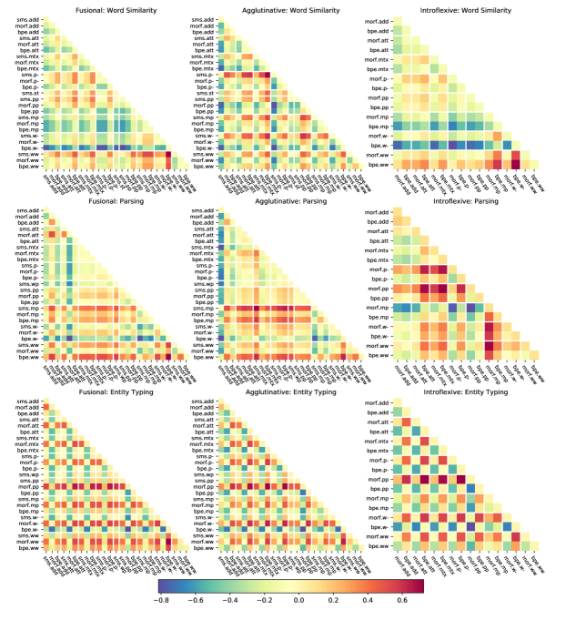
Figure 2: Comparisons of different configurations across tasks grouped by language types. The value in each pixel block is the percentage rank of the row configuration minus that of column configuration. For example, in word similarity for fusional language, the rank for the row sms.ww is $0.787$ and $0.071$ for column bpe.w-, and the block value is $0.716$. The higher the value, the better the performance of the row compared to the column configuration.

To get a better grasp of the overall performance without overloading the tables, we focus on reporting two best configurations and the worst configuration for each task and language from the total of 60 configurations, except for Hebrew with 36 configurations, where there is no gold segmentation data for training sms model. We also analyze the effects of different configurations on different tasks based on language typology. The entire analysis revolves around the key questions Q1-Q3 posed in the introduction. The reader is encouraged to refer to the supplementary material for the complete results.

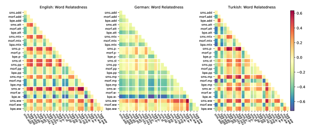
Figure 3: Comparisons of word relatedness tasks for English, German and Turkish.

Tables 4, 5, and 6 summarize the main results on word similarity and relatedness, dependency parsing and entity typing, respectively. In addition, the comparisons of different configurations across tasks and language types are shown in Figure 2 (as well as Figure 3 to 7 in the supplementary material). There, we center the comparison around two crucial components: segmentation and composition. The value in each pixel block is the percentage rank of the row configuration minus that of column configuration. We compute such percentage ranks by performing three levels of averaging over: 1) all related datasets for the same task; 2) all sub-configurations that entail the configuration in question; 3) all languages from the same language types.

Q1. Tasks and Languages

Regarding the absolute performance of our subword-informed configurations, we notice that they outperform sgns and ft in 3/5 languages on average, and for 8/13 datasets on word similarity and relatedness. The gains are more prominent over the subword-agnostic sgns model and for morphologically richer languages such as Finnish and Turkish. The results on the two other tasks are also very competitive, with strong performance reported especially on the entity typing task. This clearly indicates the importance of integrating subword-level information into word vectors. A finer-grained comparative analysis shows that best-performing configurations vary greatly across different languages.

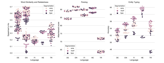
Figure 4: Results with different segmentation methods.

The comparative analysis across tasks also suggests that there is no single configuration that outperforms the others in all three tasks, although certain patterns in the results emerge. For instance, the supervised segmentation (sms) is very useful for word similarity and relatedness (seen in Figure 4). This result is quite intuitive: sms is trained according to the readily available gold standard morphological segmentations. However, sms is less useful for entity typing, where almost all best-performing configurations are based on morf (see also Figure 4). This result is also interpretable: morf is a conservative segmenter that captures longer subwords, and is not distracted by short and nonsensical subwords (like bpe) that have no contribution to the prediction. The worst configurations on word similarity are based on bpe: its aggressive segmentation often results in non-interpretable or nonsensical subwords which are unable to recover useful semantic information. Due to the same reason, the results in all three tasks indicate that the best configurations with bpe are always coupled with ww, and the worst are obtained with w- (i.e., without the inclusion of the full word).

The results on parsing reveal similar performances for a spectrum of heterogeneous configurations. In other words, while the chosen configuration is still important, its impact on performance of state-of-the-art dependency parsers Kiperwasser and Goldberg (2016); Dozat and Manning (2017) is decreased, as such parsers are heavily parametrized multi-component methods (e.g., besides word embeddings they rely on biLSTMs, intra-sentence attention, character representations). Therefore, a larger space of subword-informed configurations for word representations leads to optimal or near-optimal results. However, sms seems to yield highest scores on average in agglutinative languages (see also Figure 2).

Figure 2 clearly demonstrates that, apart from entity typing heatmaps (the third row) which show very similar trends over different language types, the patterns for different tasks and language types tend to vary in general. Similarly, other figures in the supplementary material also show diverging trends across languages representing different language types.

Q2 and Q3. Configurations

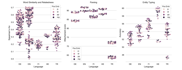
Figure 6: Results with different position embeddings.

As mentioned, different tasks reach high scores with different segmentation and composition components. The crucial components for word similarity are sms and ww, and sms is generally better than morf and bpe in fusional and agglutinative languages (see Figure 4 and 7). The presence of ww is desired in this task as also found by Bojanowski et al. (2017): it enhances the information provided by the segmentation. As discussed before, the best configurations with bpe are always coupled with ww, and the worst with w-. ww is less important for the more conservative morf where the information stored in ww can be fully recovered from the generated subwords. Interestingly, pp and mp do not have positive effects on this task for fusional and introflexive languages, but they seem to resonate well with agglutinative languages, and they are useful for the two other tasks (seen in Figure 6). In general, position embeddings have shown potential benefits in all tasks, where they selectively emphasize or filter subwords according to their positions. pp is extremely useful in entity typing for all languages, because it indicates the root position.

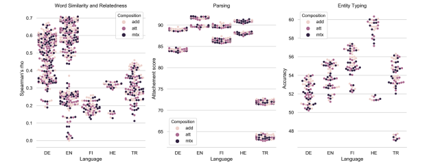
Figure 5: Results with different composition functions.

Concerning composition functions, add still remains an extremely robust choice across tasks and languages. Surprisingly, the more sophisticated self-attention composition prevails only on a handful of datasets: compare the results with add vs. att and mtx. In fact, the worst configurations mostly use att and mtx (see also Figure 5). In sum, our results suggest that, when unsure, add is by far the most robust choice for the subword composition function. Further, morphotactic tags encoded in subword embeddings (st) seem to be only effective combined with self-attention in word similarity and relatedness. These findings call for further investigation in future work, along with the inclusion of finer-grained morphotactic tags into the proposed modeling framework.

Further Discussion

A recurring theme of this study is that subword-informed configurations are largely task- and language-dependent. We can extract multiple examples from the reported results affirming this conjecture. For instance, in fusional and agglutinative languages mp is critical to the model on dependency parsing, while for Hebrew, an introflexive language, mp is among the most detrimental components on the same task. Further, for Turkish word similarity bpe.ww outperforms sms.ww: due to affix concatenation in Turkish, sms produces many affixes with only syntactic functions that bring noise to the task. Interestingly, sgns performs well in Hebrew on parsing and word similarity: it shows that it is still difficult for linear segmentation methods to capture non-concatenative morphology.

Finally, fine-tuning subword-informed representations seems especially beneficial for rare word semantics: our best configuration outperforms ft by 0.111 on card, and even surpasses all the state-of-the-art models on the rare word similarity task, as reported by Pilehvar et al. (2018). We hope that our findings on the card dataset will motivate further work on building more accurate representations for rare and unseen words Bhatia et al. (2016); Herbelot and Baroni (2017); Schick and Schütze (2018) by learning more effective and more informed components of subword-informed configurations.

5 Conclusion

We have presented a general framework for learning subword-informed word representations which has been used to perform a systematic analysis of 60 different subword-aware configurations for 5 typologically diverse languages across 3 diverse tasks. The large space of presented results has allowed us to analyze the main properties of subword-informed representation learning: we have demonstrated that different components of the framework such as segmentation and composition methods, or the use of position embeddings, have to be carefully tuned to yield improved performance across different tasks and languages. We hope that this study will guide the development of new subword-informed word representation architectures. Code is available at: https://github.com/cambridgeltl/sw_study.

Appendix A Supplemental Material

In this supplementary material we present the full results of different configurations of our subword-informed representations and baseline models in three tasks across five languages. For details and notations of different model configurations, please refer to the original paper.

Since fastText (ft) package cannot generate each subword embedding for a given word, we also implemented our own version (our_ft) within the same subword-informed training framework. We trained our_ft on all the five languages with the same training corpus, and kept the same hyperparameters as ft package except that we used 1024 as batch size for faster training. We show that our implementation yields comparable results with the original ft in word similarity and relatedness and parsing across languages. For entity typing, we experimented with the extended hierarchical composition architecture described in the paper on our_ft, i.e., using subword embeddings to compute word representations and updating subword embeddings of our_ft during training, and only use word embeddings as input for sgns and ft and directly update them. Additionally, we also experimented with some of our model configurations with character n-grams as our segmentation methods, but did not observe performance gains. Due to its large parameter space (usually 2-4 times larger than sgns) and the computational limits, we leave it as our future work.

Table 7, 8 and 9 show the results of word similarity and relatedness based on different segmentation methods, and Table 10, 11 and 12 for the results of dependency parsing. Table 13 shows the accuracy on development and test set for entity typing across all five languages. Figure 3 shows the configuration comparisons in languages with available datasets for word relatedness. Figure 4 to 7 show the results on all downstream tasks across languages when each test data point is categorized according to some specific component. Specifically, Figure 4 shows the results when only different segmentation methods are considered, and Figure 5, 6 and 7 show the results on varying composition functions, position embedding types and whether including the word token embedding, respectively.

	simlex	ws	ws-rel	ws-sim	fs300	an-rel	an-sim	card
sms.w-.p-.add	0.267(en)	0.650	0.625	0.688	0.259(fi)	0.277(tr)	0.432(tr)	0.206(en)
	0.350(de)	0.517	0.490	0.586
sms.w-.st.add	0.267	0.654	0.619	0.704	0.228	0.276	0.434	0.208
	0.350	0.509	0.475	0.577
sms.w-.pp.add	0.270	0.645	0.615	0.693	0.258	0.261	0.444	0.294
	0.332	0.494	0.467	0.563
sms.w-.mp.add	0.207	0.635	0.598	0.683	0.247	0.269	0.424	0.213
	0.295	0.437	0.401	0.507
sms.ww.p-.add	0.283	0.640	0.589	0.696	0.226	0.273	0.435	0.267
	0.401	0.633	0.616	0.668
sms.ww.st.add	0.277	0.637	0.576	0.697	0.204	0.239	0.404	0.269
	0.385	0.622	0.601	0.658
sms.ww.pp.add	0.282	0.632	0.572	0.702	0.240	0.240	0.423	0.370
	0.398	0.633	0.610	0.673
sms.ww.mp.add	0.240	0.633	0.579	0.696	0.211	0.279	0.443	0.268
	0.353	0.599	0.557	0.639
sms.w-.p-.att	0.250	0.642	0.613	0.684	0.228	0.289	0.416	0.244
	0.339	0.518	0.478	0.598
sms.w-.st.att	0.255	0.656	0.620	0.697	0.227	0.263	0.358	0.236
	0.327	0.512	0.468	0.583
sms.w-.pp.att	0.252	0.655	0.619	0.707	0.227	0.212	0.334	0.323
	0.324	0.500	0.456	0.570
sms.w-.mp.att	0.206	0.629	0.593	0.674	0.205	0.263	0.405	0.219
	0.290	0.452	0.425	0.517
sms.ww.p-.att	0.277	0.642	0.591	0.698	0.192	0.311	0.440	0.251
	0.360	0.605	0.571	0.640
sms.ww.st.att	0.261	0.632	0.570	0.693	0.212	0.243	0.366	0.260
	0.342	0.588	0.549	0.625
sms.ww.pp.att	0.271	0.630	0.584	0.695	0.228	0.204	0.367	0.310
	0.357	0.608	0.567	0.660
sms.ww.mp.att	0.220	0.616	0.547	0.682	0.191	0.241	0.376	0.222
	0.340	0.569	0.526	0.613
sms.w-.p-.mtx	0.245	0.639	0.602	0.694	0.248	0.260	0.404	0.220
	0.336	0.505	0.457	0.585
sms.w-.st.mtx	0.252	0.648	0.617	0.702	0.234	0.231	0.381	0.224
	0.330	0.506	0.456	0.578
sms.w-.pp.mtx	0.260	0.638	0.606	0.694	0.244	0.184	0.335	0.328
	0.331	0.488	0.429	0.564
sms.w-.mp.mtx	0.211	0.620	0.599	0.671	0.228	0.265	0.417	0.226
	0.282	0.447	0.417	0.506
sms.ww.p-.mtx	0.279	0.631	0.575	0.696	0.206	0.280	0.426	0.251
	0.357	0.615	0.578	0.657
sms.ww.st.mtx	0.277	0.642	0.581	0.708	0.192	0.231	0.394	0.261
	0.355	0.603	0.561	0.645
sms.ww.pp.mtx	0.273	0.640	0.588	0.705	0.226	0.210	0.368	0.300
	0.357	0.611	0.575	0.662
sms.ww.mp.mtx	0.253	0.622	0.565	0.684	0.183	0.275	0.414	0.260
	0.339	0.598	0.578	0.632
sgns	0.300	0.634	0.579	0.702	0.211	0.232	0.183	0.009
	0.359	0.596	0.530	0.669
ft	0.307	0.643	0.586	0.706	0.279	0.271	0.520	0.249
	0.393	0.624	0.590	0.677
our_ft	0.265	0.629	0.574	0.702	0.241	0.295	0.523	0.281
	0.380	0.610	0.596	0.649

Table 7: Results on word similarity and relatedness across languages for CHIPMUNK (sms). All scores are obtained after computing the embeddings of OOV words.

	simlex	ws	ws-rel	ws-sim	fs300	an-rel	an-sim	card
morf.w-.p-.add	0.282(en)	0.629	0.574	0.691	0.166(fi)	0.273(tr)	0.359(tr)	0.134(en)
	0.368(de)	0.577	0.557	0.616
	0.322(he)
morf.w-.pp.add	0.279	0.617	0.562	0.680	0.189	0.232	0.375	0.172
	0.349	0.549	0.530	0.594
	0.317
morf.w-.mp.add	0.245	0.597	0.529	0.664	0.185	0.302	0.351	0.127
	0.303	0.484	0.439	0.550
	0.324
morf.ww.p-.add	0.273	0.632	0.573	0.697	0.159	0.264	0.339	0.198
	0.376	0.583	0.569	0.614
	0.326
morf.ww.pp.add	0.277	0.616	0.557	0.684	0.182	0.232	0.375	0.262
	0.361	0.573	0.549	0.609
	0.324
morf.ww.mp.add	0.244	0.589	0.520	0.666	0.149	0.267	0.300	0.099
	0.331	0.515	0.484	0.574
	0.304
morf.w-.p-.att	0.281	0.623	0.565	0.682	0.159	0.295	0.362	0.132
	0.354	0.560	0.536	0.603
	0.323
morf.w-.pp.att	0.276	0.619	0.555	0.682	0.170	0.235	0.358	0.138
	0.352	0.556	0.537	0.597
	0.308
morf.w-.mp.att	0.246	0.586	0.519	0.661	0.158	0.274	0.304	0.107
	0.310	0.495	0.453	0.548
	0.291
morf.ww.p-.att	0.271	0.622	0.568	0.686	0.167	0.292	0.346	0.218
	0.372	0.574	0.545	0.621
	0.321
morf.ww.pp.att	0.274	0.613	0.549	0.680	0.167	0.145	0.312	0.206
	0.364	0.565	0.537	0.601
	0.319
morf.ww.mp.att	0.234	0.586	0.514	0.666	0.147	0.270	0.273	0.109
	0.327	0.499	0.469	0.562
	0.307
morf.w-.p-.mtx	0.280	0.632	0.573	0.693	0.133	0.300	0.357	0.132
	0.348	0.564	0.544	0.602
	0.320
morf.w-.pp.mtx	0.275	0.621	0.562	0.693	0.186	0.231	0.369	0.135
	0.355	0.549	0.530	0.582
	0.325
morf.w-.mp.mtx	0.254	0.602	0.536	0.671	0.205	0.235	0.295	0.130
	0.295	0.488	0.427	0.542
	0.301
morf.ww.p-.mtx	0.275	0.624	0.558	0.688	0.177	0.292	0.356	0.222
	0.371	0.577	0.545	0.611
	0.325
morf.ww.pp.mtx	0.272	0.617	0.558	0.684	0.160	0.151	0.321	0.080
	0.359	0.592	0.575	0.613
	0.326
morf.ww.mp.mtx	0.238	0.591	0.522	0.674	0.123	0.279	0.326	0.080
	0.320	0.500	0.465	0.559
	0.318
sgns	0.300	0.634	0.579	0.702	0.211	0.232	0.183	0.009
	0.359	0.596	0.530	0.669
	0.379
ft	0.307	0.643	0.586	0.706	0.279	0.271	0.520	0.249
	0.393	0.624	0.590	0.677
	0.388
our_ft	0.265	0.629	0.574	0.702	0.241	0.295	0.523	0.281
	0.380	0.610	0.596	0.649
	0.354

Table 8: Results on word similarity and relatedness across languages for Morfessor (morf). All scores are obtained after computing the embeddings of OOV words.

	simlex	ws	ws-rel	ws-sim	fs300	an-rel	an-sim	card
bpe.w-.p-.add	0.209(en)	0.488	0.499	0.508	0.177(fi)	0.228(tr)	0.390(tr)	0.011(en)
	0.229(de)	0.416	0.442	0.474
	0.156(he)
bpe.w-.pp.add	0.209	0.474	0.484	0.490	0.170	0.229	0.407	0.000
	0.225	0.404	0.417	0.467
	0.162
bpe.w-.mp.add	0.182	0.460	0.478	0.484	0.157	0.283	0.406	0.021
	0.193	0.331	0.351	0.363
	0.132
bpe.ww.p-.add	0.274	0.642	0.577	0.706	0.203	0.293	0.429	0.262
	0.378	0.597	0.582	0.631
	0.331
bpe.ww.pp.add	0.265	0.631	0.571	0.689	0.245	0.267	0.429	0.273
	0.365	0.615	0.595	0.637
	0.338
bpe.ww.mp.add	0.236	0.587	0.519	0.658	0.147	0.355	0.459	0.240
	0.348	0.566	0.538	0.608
	0.321
bpe.w-.p-.att	0.216	0.506	0.504	0.529	0.200	0.176	0.288	0.010
	0.233	0.386	0.409	0.422
	0.155
bpe.w-.pp.att	0.210	0.503	0.507	0.528	0.190	0.183	0.331	0.027
	0.226	0.383	0.396	0.428
	0.152
bpe.w-.mp.att	0.197	0.456	0.462	0.475	0.173	0.200	0.308	0.035
	0.209	0.398	0.422	0.467
	0.151
bpe.ww.p-.att	0.265	0.621	0.566	0.687	0.197	0.246	0.358	0.257
	0.350	0.555	0.525	0.591
	0.334
bpe.ww.pp.att	0.270	0.618	0.570	0.678	0.187	0.197	0.314	0.228
	0.333	0.567	0.536	0.604
	0.334
bpe.ww.mp.att	0.255	0.613	0.564	0.681	0.147	0.325	0.419	0.226
	0.338	0.545	0.526	0.584
	0.307
bpe.w-.p-.mtx	0.202	0.486	0.485	0.512	0.184	0.174	0.293	0.015
	0.224	0.394	0.414	0.433
	0.169
bpe.w-.pp.mtx	0.198	0.504	0.500	0.547	0.179	0.195	0.355	0.045
	0.223	0.399	0.396	0.462
	0.167
bpe.w-.mp.mtx	0.185	0.440	0.438	0.476	0.144	0.176	0.282	0.022
	0.189	0.328	0.332	0.372
	0.128
bpe.ww.p-.mtx	0.267	0.624	0.565	0.690	0.164	0.238	0.334	0.272
	0.354	0.573	0.543	0.604
	0.337
bpe.ww.pp.mtx	0.263	0.621	0.569	0.677	0.193	0.112	0.290	0.210
	0.337	0.553	0.500	0.608
	0.338
bpe.ww.mp.mtx	0.260	0.620	0.564	0.681	0.198	0.257	0.369	0.247
	0.336	0.546	0.514	0.596
	0.298
sgns	0.300	0.634	0.579	0.702	0.211	0.232	0.183	0.009
	0.359	0.596	0.530	0.669
	0.379
ft	0.307	0.643	0.586	0.706	0.279	0.271	0.520	0.249
	0.393	0.624	0.590	0.677
	0.388
our_ft	0.265	0.629	0.574	0.702	0.241	0.295	0.523	0.281
	0.380	0.610	0.596	0.649
	0.354

Table 9: Results on word similarity and relatedness across languages for BPE (bpe). All scores are obtained after computing the embeddings of OOV words.

	dev(en)	test	dev(de)	test	dev(fi)	test	dev(tr)	test
sms.w-.p-.add	92.2(uas)	91.5	91.3	89.0	88.8	89.6	70.0	71.9
	90.3(las)	89.6	87.7	84.2	85.5	86.1	62.1	63.7
sms.w-.st.add	92.4	91.7	91.1	88.7	89.1	89.7	71.0	72.0
	90.5	89.7	87.6	83.8	86.0	86.6	62.9	63.8
sms.w-.pp.add	92.2	91.9	91.4	88.7	89.3	90.5	70.9	72.7
	90.2	89.9	87.8	84.0	86.1	87.1	62.8	64.4
sms.w-.mp.add	92.2	91.9	91.1	89.1	89.0	89.9	70.5	72.6
	90.3	90.0	87.6	84.3	85.8	86.6	62.6	64.5
sms.ww.p-.add	92.2	92.1	91.6	89.1	89.4	90.1	71.0	71.8
	90.2	90.0	88.1	84.3	86.4	86.9	62.8	63.6
sms.ww.st.add	92.4	91.9	91.3	89.2	89.4	89.9	71.0	72.0
	90.5	89.8	87.9	84.5	86.2	86.5	63.0	64.0
sms.ww.pp.add	92.5	91.9	91.3	88.9	89.5	90.3	70.7	72.5
	90.5	90.0	87.8	84.2	86.5	87.0	63.0	64.4
sms.ww.mp.add	92.2	91.7	91.4	89.2	89.4	90.3	71.1	72.8
	90.3	89.6	87.8	84.4	86.3	87.1	63.5	64.7
sms.w-.p-.att	92.1	91.7	91.3	88.9	89.0	89.6	71.3	72.4
	90.2	89.6	87.7	83.9	85.9	86.4	63.1	63.8
sms.w-.st.att	92.2	91.6	91.4	89.0	88.8	89.4	70.0	71.9
	90.3	89.6	87.7	84.2	85.6	86.0	62.2	63.4
sms.w-.pp.att	91.4	91.2	91.1	89.0	89.2	89.7	70.7	71.4
	89.4	89.0	87.6	84.3	85.7	86.1	62.6	63.0
sms.w-.mp.att	92.1	91.8	91.3	89.0	89.0	90.0	70.5	72.7
	90.2	89.8	87.7	84.1	85.9	86.6	62.5	64.5
sms.ww.p-.att	92.1	91.5	91.2	89.3	89.2	89.8	71.2	72.3
	90.2	89.6	87.7	84.5	85.9	86.4	63.2	64.0
sms.ww.st.att	92.3	91.9	91.3	89.2	88.7	89.7	70.4	72.2
	90.4	89.9	87.8	84.3	85.5	86.2	62.3	63.8
sms.ww.pp.att	92.2	91.8	91.5	89.0	88.5	89.3	71.0	72.2
	90.3	89.8	87.9	84.4	84.9	85.8	62.7	63.7
sms.ww.mp.att	92.3	91.9	91.5	89.1	88.6	89.5	70.7	72.5
	90.5	90.0	88.0	84.3	85.4	86.0	62.9	64.3
sms.w-.p-.mtx	92.0	91.9	91.5	88.6	89.0	89.7	70.5	71.7
	90.1	89.8	87.9	83.7	85.9	86.2	62.5	63.5
sms.w-.st.mtx	92.1	91.8	91.1	88.5	89.0	89.5	69.8	71.8
	90.2	89.7	87.8	83.5	85.6	85.9	61.8	63.3
sms.w-.pp.mtx	92.3	91.7	91.2	89.1	88.9	89.6	70.7	72.0
	90.4	89.7	87.6	84.2	85.9	86.3	62.6	63.1
sms.w-.mp.mtx	92.3	92.0	91.4	89.1	89.4	90.2	70.7	72.4
	90.3	90.1	87.8	84.3	86.0	86.9	62.5	64.2
sms.ww.p-.mtx	92.2	91.6	91.4	89.1	89.2	89.8	70.5	71.9
	90.4	89.6	87.9	84.3	86.0	86.4	62.5	63.6
sms.ww.st.mtx	92.2	91.6	91.4	88.7	89.1	89.8	71.0	71.8
	90.4	89.7	87.8	83.9	85.8	86.5	62.7	63.3
sms.ww.pp.mtx	92.3	92.0	91.2	89.0	88.7	89.4	70.4	71.8
	90.4	89.9	87.7	84.2	85.2	85.8	62.7	63.6
sms.ww.mp.mtx	92.3	92.0	91.4	88.9	88.8	89.6	71.0	71.5
	90.4	89.9	87.8	84.0	85.2	85.9	62.7	63.3
sgns	92.3	91.9	91.4	89.3	88.9	89.5	70.5	72.2
	90.4	89.8	87.9	84.4	85.6	86.2	62.5	63.5
ft	92.3	92.1	91.6	89.1	89.7	90.4	71.2	73.1
	90.3	90.2	87.9	84.4	86.9	87.1	63.3	65.1
our_ft	92.7	92.2	91.6	89.6	90.5	90.9	71.5	73.0
	90.7	90.2	87.9	84.9	87.6	87.8	63.5	64.9

Table 10: Results on dependency parsing across languages for CHIPMUNK (sms).

	dev(en)	test	dev(de)	test	dev(fi)	test	dev(tr)	test	dev(he)	test
morf.w-.p-.add	92.3	91.7	91.1	89.0	89.0	90.0	70.7	71.8	92.5	91.0
	90.4	89.8	87.7	84.2	85.8	86.6	62.4	63.3	89.6	88.3
morf.w-.pp.add	92.5	91.8	91.4	89.0	89.2	89.8	70.3	71.3	92.3	91.2
	90.6	89.8	87.6	84.1	86.0	86.4	62.2	63.1	89.6	88.4
morf.w-.mp.add	92.2	91.9	91.4	89.0	89.2	89.8	71.2	71.7	92.1	90.8
	90.2	90.0	87.8	84.1	85.9	86.4	63.2	63.6	89.2	88.0
morf.ww.p-.add	92.2	91.8	91.4	89.0	89.4	89.6	70.8	72.2	92.3	91.2
	90.3	89.7	87.8	84.1	86.2	86.2	62.9	64.2	89.5	88.5
morf.ww.pp.add	92.3	91.7	91.3	88.9	88.8	89.9	70.6	71.9	92.2	91.0
	90.4	89.8	87.6	84.1	85.7	86.5	62.5	63.4	89.6	88.1
morf.ww.mp.add	92.3	91.7	91.2	89.0	89.3	89.8	70.5	72.4	92.1	90.9
	90.4	89.6	87.6	84.2	86.0	86.4	62.8	64.2	89.2	88.0
morf.w-.p-.att	92.2	91.8	91.2	89.1	89.1	90.2	70.3	72.1	92.3	91.1
	90.3	89.7	87.6	83.9	85.9	86.6	61.9	63.6	89.6	88.3
morf.w-.pp.att	92.3	92.0	91.5	89.3	89.1	89.7	71.0	72.2	92.6	91.2
	90.3	89.9	87.9	84.6	85.9	86.4	63.1	63.6	89.7	88.4
morf.w-.mp.att	92.0	91.8	91.4	89.1	89.1	89.9	70.2	71.5	92.1	90.3
	90.0	89.8	87.7	84.3	85.7	86.4	62.1	62.8	89.2	87.4
morf.ww.p-.att	92.2	91.9	91.4	89.1	89.4	89.8	70.0	71.2	92.2	91.1
	90.2	89.8	88.0	84.2	86.0	86.5	62.2	62.8	89.3	88.2
morf.ww.pp.att	92.3	91.9	91.6	89.3	89.0	89.6	70.9	72.0	92.2	91.1
	90.3	89.9	88.0	84.5	85.8	86.3	62.7	63.4	89.6	88.3
morf.ww.mp.att	92.2	91.9	91.3	89.0	88.9	90.0	70.9	71.8	92.3	91.0
	90.4	90.0	87.9	84.1	85.8	86.7	62.8	63.4	89.4	88.0
morf.w-.p-.mtx	92.1	91.9	91.4	88.9	89.3	89.8	70.6	71.9	92.2	90.6
	90.1	89.8	87.8	84.1	86.1	86.4	62.8	63.6	89.4	87.9
morf.w-.pp.mtx	92.4	91.8	91.3	88.8	89.3	90.0	71.0	72.2	92.3	91.3
	90.4	89.9	87.7	84.0	86.1	86.7	63.1	63.7	89.5	88.5
morf.w-.mp.mtx	92.2	92.1	91.4	88.8	89.2	90.3	70.2	72.2	92.2	90.5
	90.3	90.0	87.9	83.9	85.9	86.8	62.2	63.7	89.3	87.7
morf.ww.p-.mtx	92.2	91.8	91.3	88.9	89.3	89.6	70.1	71.4	92.5	91.4
	90.3	89.8	87.9	84.0	85.9	86.1	62.1	63.3	89.6	88.4
morf.ww.pp.mtx	92.2	91.7	91.4	89.0	89.2	89.9	71.3	72.1	92.6	90.8
	90.3	89.6	87.9	84.1	86.0	86.7	62.9	63.8	89.7	88.0
morf.ww.mp.mtx	92.3	91.8	91.2	89.1	89.5	89.8	71.1	72.2	92.1	90.8
	90.4	89.9	87.7	84.2	86.3	86.4	62.5	63.8	89.3	88.0
sgns	92.3	91.9	91.4	89.3	88.9	89.5	70.5	72.2	92.4	91.5
	90.4	89.8	87.9	84.4	85.6	86.2	62.5	63.5	89.8	88.7
ft	92.3	92.1	91.6	89.1	89.7	90.4	71.2	73.1	92.6	91.2
	90.3	90.2	87.9	84.4	86.9	87.1	63.3	65.1	89.7	88.3
our_ft	92.7	92.2	91.6	89.6	90.5	90.9	71.5	73.0	92.52	91.6
	90.7	90.2	87.9	84.9	87.6	87.8	63.5	64.9	89.72	88.8

Table 11: Results on dependency parsing across languages for Morfessor (morf).

	dev(en)	test	dev(de)	test	dev(fi)	test	dev(tr)	test	dev(he)	test
bpe.w-.p-.add	92.3	91.5	91.1	89.1	89.3	89.9	70.2	72.1	91.9	91.0
	90.3	89.6	87.6	84.2	85.9	86.4	62.6	63.9	89.2	88.2
bpe.w-.pp.add	92.2	91.6	91.5	89.1	89.0	90.0	71.2	71.6	92.0	90.9
	90.2	89.5	87.9	84.3	85.8	86.7	63.2	63.2	89.1	88.1
bpe.w-.mp.add	91.9	91.6	91.5	89.2	89.3	89.8	70.7	71.6	92.4	91.2
	90.0	89.7	87.9	84.3	86.1	86.3	62.7	63.4	89.7	88.2
bpe.ww.p-.add	92.1	91.8	91.3	89.2	89.5	89.8	70.2	71.4	92.5	91.1
	90.2	89.9	87.7	84.4	86.2	86.5	62.1	63.2	89.5	88.2
bpe.ww.pp.add	92.3	91.6	91.2	89.6	89.2	90.2	70.8	72.3	92.3	91.2
	90.4	89.6	87.7	84.7	86.2	87.0	62.9	64.2	89.4	88.4
bpe.ww.mp.add	92.3	91.9	91.6	89.2	89.9	90.7	71.2	72.3	92.2	91.0
	90.3	89.9	88.1	84.5	86.9	87.4	63.1	64.0	89.4	88.2
bpe.w-.p-.att	92.3	91.3	91.4	89.1	88.8	89.4	70.4	71.9	92.0	90.9
	90.3	89.4	87.9	84.2	85.3	85.7	62.3	63.0	89.1	87.9
bpe.w-.pp.att	92.1	91.6	91.4	88.6	88.7	89.5	70.9	71.5	91.9	91.0
	90.2	89.7	87.6	83.7	85.4	86.0	62.5	63.3	89.0	88.3
bpe.w-.mp.att	92.1	91.5	91.5	89.3	89.1	89.9	70.5	72.4	92.2	90.8
	90.2	89.6	87.9	84.4	85.8	86.3	62.5	63.9	89.5	88.0
bpe.ww.p-.att	92.3	92.0	91.4	88.6	89.1	90.1	70.8	71.3	92.0	90.8
	90.4	89.9	87.9	83.8	85.8	86.8	62.4	63.1	89.3	88.0
bpe.ww.pp.att	92.3	91.8	91.4	89.2	89.2	90.0	71.0	72.1	92.1	91.1
	90.5	89.8	87.7	84.6	85.9	86.4	63.2	64.0	89.5	88.2
bpe.ww.mp.att	92.5	92.0	91.5	89.3	89.5	90.3	70.6	71.7	91.9	90.9
	90.6	89.9	88.1	83.9	86.4	86.9	62.6	63.4	89.1	88.0
bpe.w-.p-.mtx	91.9	91.7	91.1	88.9	88.6	89.5	69.9	71.5	91.5	91.2
	90.1	89.7	87.5	83.9	85.2	85.9	61.9	63.1	88.7	88.3
bpe.w-.pp.mtx	92.1	91.7	91.1	88.8	89.0	89.5	70.7	71.8	92.0	91.0
	90.2	89.7	87.5	84.0	85.6	86.0	62.8	63.3	89.2	88.2
bpe.w-.mp.mtx	92.1	91.6	91.1	89.1	89.0	89.9	70.3	72.0	92.2	90.6
	90.2	89.5	87.6	84.1	85.7	86.3	62.6	63.6	89.3	87.7
bpe.ww.p-.mtx	92.3	92.1	91.6	89.0	89.3	90.0	71.7	72.3	91.9	90.5
	90.4	90.0	88.0	84.2	86.0	86.7	63.4	63.7	88.9	87.7
bpe.ww.pp.mtx	92.4	91.9	91.3	89.1	89.3	89.7	69.8	72.2	92.0	90.7
	90.4	89.8	87.7	84.2	85.9	86.2	62.0	63.8	89.2	87.9
bpe.ww.mp.mtx	92.3	91.7	91.2	89.4	89.8	90.2	71.2	72.3	92.2	91.0
	90.4	89.6	87.7	84.7	86.7	86.8	63.1	64.2	89.4	88.1
sgns	92.3	91.9	91.4	89.3	88.9	89.5	70.5	72.2	92.4	91.5
	90.4	89.8	87.9	84.4	85.6	86.2	62.5	63.5	89.8	88.7
ft	92.3	92.1	91.6	89.1	89.7	90.4	71.2	73.1	92.6	91.2
	90.3	90.2	87.9	84.4	86.9	87.1	63.3	65.1	89.7	88.3
our_ft	92.7	92.2	91.6	89.6	90.5	90.9	71.5	73.0	92.52	91.6
	90.7	90.2	87.9	84.9	87.6	87.8	63.5	64.9	89.72	88.8

Table 12: Results on dependency parsing across languages for BPE (bpe).

	dev(en)	test	dev(de)	test	dev(fi)	test	dev(tr)	test	dev(he)	test
sms.w-.p-.add	52.88	52.57	51.09	50.95	55.15	55.08	53.87	53.52
sms.w-.st.add	52.68	52.7	51.2	51.23	55.38	55.13	54.03	53.68
sms.w-.pp.add	53.19	52.94	50.48	50.83	55.44	55.30	54.05	53.88
sms.w-.mp.add	52.87	52.76	51.1	51.11	55.18	55.00	54.24	53.96
sms.ww.p-.add	53.56	53.69	51.73	51.77	55.92	55.84	55.01	54.76
sms.ww.st.add	54.21	54.26	52.53	52.63	56.21	55.95	55.96	55.43
sms.ww.pp.add	54.51	54.66	52.98	53.04	56.06	56.00	55.92	55.75
sms.ww.mp.add	54.27	54.43	52.77	52.88	56.04	55.71	56.38	55.99
sms.w-.p-.att	52.81	52.7	50.7	50.8	54.85	54.67	53.62	53.45
sms.w-.st.att	52.57	52.64	51.64	51.65	54.87	54.69	53.27	53.14
sms.w-.pp.att	52.94	52.66	52.1	52.5	54.91	54.83	53.39	53.21
sms.w-.mp.att	52.99	52.91	51.7	51.9	55.02	55.03	54.06	53.72
sms.ww.p-.att	53.68	53.67	51.48	51.69	55.59	55.73	55.17	54.92
sms.ww.st.att	53.55	53.66	51.64	51.65	55.27	55.35	53.84	53.26
sms.ww.pp.att	53.14	53.08	52.1	52.5	54.66	54.52	54.95	54.77
sms.ww.mp.att	53.82	53.79	51.67	51.89	54.02	54.04	54.1	53.76
sms.w-.p-.mtx	52.7	52.67	50.29	50.52	54.61	54.51	53.44	53.24
sms.w-.st.mtx	52.75	52.61	50.42	50.85	54.15	54.09	53.44	52.84
sms.w-.pp.mtx	52.89	52.87	51.07	51.38	54.58	54.70	53.42	53.16
sms.w-.mp.mtx	53.03	52.89	50.52	50.95	55.19	54.90	54.23	53.68
sms.ww.p-.mtx	53.75	53.81	51.47	51.48	55.34	55.37	54.51	54.36
sms.ww.st.mtx	53.75	53.64	51.24	51.51	55.4	55.36	54.97	54.72
sms.ww.pp.mtx	53.80	53.96	51.92	52.1	54.57	54.54	54.94	54.57
sms.ww.mp.mtx	54.23	54.2	52	52.2	55.02	54.84	55.8	55.45
morf.w-.p-.add	54.86	55.35	53.41	53.28	57.01	56.94	55.92	55.8	60.37	59.67
morf.w-.pp.add	55.55	55.57	54.02	54.06	57.69	57.41	56.79	56.31	60.61	59.99
morf.w-.mp.add	55.01	55.18	53.5	53.35	57.09	56.82	55.26	54.7	60.1	59.24
morf.ww.p-.add	54.94	55.09	53.27	53.02	56.61	56.55	55.5	54.9	60.23	59.65
morf.ww.pp.add	55.20	55.60	53.83	53.82	57.32	57.2	56.41	55.92	60.57	60.09
morf.ww.mp.add	54.63	54.67	53.46	53.4	56.81	56.73	54.42	53.88	59.67	58.87
morf.w-.p-.att	54.84	55.02	52.98	52.91	56.93	56.83	55.86	55.52	60.3	59.78
morf.w-.pp.att	55.28	55.68	53.92	54.01	57.36	57.24	56.62	56.13	60.83	60.34
morf.w-.mp.att	55.4	55.3	53.72	53.7	56.85	56.93	55.24	54.6	59.89	59.38
morf.ww.p-.att	54.94	54.87	53.07	53.12	56.7	56.36	55.5	55.07	60.31	59.73
morf.ww.pp.att	55.26	55.35	53.83	53.92	57.39	57.15	56.39	55.99	60.5	59.94
morf.ww.mp.att	55.16	55.27	53.22	53.26	56.84	56.67	54.89	54.32	59.59	59.04
morf.w-.p-.mtx	54.97	55.06	52.39	52.42	56.76	56.88	55.93	55.39	60.26	59.66
morf.w-.pp.mtx	55.18	55.4	53.95	53.92	57.49	57.38	56.62	56.14	60.65	60.02
morf.w-.mp.mtx	55.18	55.25	52.92	53.01	56.97	56.69	55.02	54.48	60.07	59.36
morf.ww.p-.mtx	54.9	55.07	53.06	53.07	56.61	56.63	55.6	54.87	60.3	59.65
morf.ww.pp.mtx	55.25	55.45	53.64	53.55	57.31	57.17	56.28	55.86	60.52	59.98
morf.ww.mp.mtx	55.1	55.16	53.43	53.4	56.81	56.69	54.57	53.89	59.71	58.95
bpe.w-.p-.add	50.74	51.3	50.43	50.42	52.74	52.53	47.85	47.6	51.67	51.44
bpe.w-.pp.add	50.92	51.59	50.77	50.68	52.93	52.74	48.32	47.71	51.65	51.33
bpe.w-.mp.add	51.35	51.93	51	50.81	53.37	53.1	47.71	47.3	52.07	51.78
bpe.ww.p-.add	54.6	55.01	53.45	53.39	56.38	55.96	53.35	53.05	59.53	59.03
bpe.ww.pp.add	54.86	55.03	53.47	53.53	56.65	56.27	53.03	52.71	59.95	59.26
bpe.ww.mp.add	55.28	55.7	53.90	53.61	57.14	56.82	53.9	53.52	60.1	59.24
bpe.w-.p-.att	50.65	51.15	50.35	50.21	52.71	52.18	47.52	47.05	51.45	51.31
bpe.w-.pp.att	50.85	51.57	50.66	50.45	52.94	52.47	47.94	47.58	51.71	51.35
bpe.w-.mp.att	51.28	51.94	50.92	50.89	53.13	52.93	47.51	47.21	52.05	51.69
bpe.ww.p-.att	53.19	53.49	51.99	52.09	54.96	54.71	52.3	52.37	57.6	57.17
bpe.ww.pp.att	53.18	53.56	52.13	51.92	55.13	54.91	53.41	53.29	58.67	57.96
bpe.ww.mp.att	54.23	54.71	52.88	52.78	55.85	55.64	53.02	53.15	58.87	58.21
bpe.w-.p-.mtx	50.81	51.48	50.42	50.33	52.76	52.36	47.58	47.14	51.67	51.34
bpe.w-.pp.mtx	51.05	51.79	50.53	50.4	52.89	52.29	47.36	46.97	51.79	51.46
bpe.w-.mp.mtx	51.45	51.88	51.15	50.93	53.27	52.93	47.7	47.34	52.18	51.87
bpe.ww.p-.mtx	53.19	53.49	52.35	52.07	55.15	54.77	52.87	52.6	58.43	57.84
bpe.ww.pp.mtx	53.17	53.57	52.35	52.18	55.08	54.58	52.44	52.02	57.92	57.43
bpe.ww.mp.mtx	54.64	55.05	53.11	52.86	55.73	55.49	53.34	53.11	59.16	58.37
sgns	50.56	51	50.55	50.14	49.88	49.87	55.09	54.35	54.93	54.55
ft	54.97	55.15	54.46	54.55	57.18	57.18	55.46	54.62	59.67	59.09
our_ft	54.59	55.12	54.26	54.4	57.67	57.57	56.19	55.73	60.05	59.65

Table 13: Accuracy on fine-grained entity typing across languages.

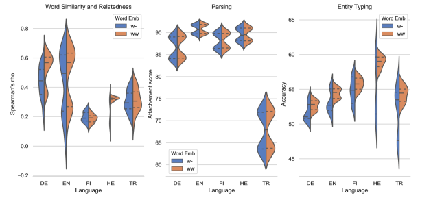
Figure 7: Results w/o word token embedding.

References

- Ammar et al. (2016) Waleed Ammar, George Mulcaire, Miguel Ballesteros, Chris Dyer, and Noah A. Smith. 2016. Many languages, one parser. Transactions of the ACL, 4:431–444.
- Avraham and Goldberg (2017) Oded Avraham and Yoav Goldberg. 2017. The interplay of semantics and morphology in word embeddings. In Proceedings of EACL, pages 422–426.
- Bhatia et al. (2016) Parminder Bhatia, Robert Guthrie, and Jacob Eisenstein. 2016. Morphological priors for probabilistic neural word embeddings. In Proceedings of EMNLP, pages 490–500.
- Bojanowski et al. (2017) Piotr Bojanowski, Edouard Grave, Armand Joulin, and Tomas Mikolov. 2017. Enriching word vectors with subword information. Transactions of the ACL, 5:135–146.
- Chaudhary et al. (2018) Aditi Chaudhary, Chunting Zhou, Lori Levin, Graham Neubig, David R. Mortensen, and Jaime Carbonell. 2018. Adapting word embeddings to new languages with morphological and phonological subword representations. In Proceedings of EMNLP, pages 3285–3295.
- Chen and Manning (2014) Danqi Chen and Christopher Manning. 2014. A fast and accurate dependency parser using neural networks. In Proceedings of EMNLP, pages 740–750.
- Collobert et al. (2011) Ronan Collobert, Jason Weston, Léon Bottou, Michael Karlen, Koray Kavukcuoglu, and Pavel Kuksa. 2011. Natural language processing (almost) from scratch. Journal of Machine Learning Research, 12:2493–2537.
- Cotterell et al. (2015) Ryan Cotterell, Thomas Müller, Alexander M. Fraser, and Hinrich Schütze. 2015. Labeled morphological segmentation with semi-Markov models. In Proceedings of CoNLL, pages 164–174.
- Cotterell and Schütze (2015) Ryan Cotterell and Hinrich Schütze. 2015. Morphological word-embeddings. In Proceedings of NAACL, pages 1287–1292.
- Cotterell and Schütze (2018) Ryan Cotterell and Hinrich Schütze. 2018. Joint semantic synthesis and morphological analysis of the derived word. Transactions of the ACL, 6:33–48.
- Dozat and Manning (2017) Timothy Dozat and Christopher D. Manning. 2017. Deep biaffine attention for neural dependency parsing. In Proceedings of ICLR.
- Dozat et al. (2017) Timothy Dozat, Peng Qi, and Christopher D. Manning. 2017. Stanford’s graph-based neural dependency parser at the CoNLL 2017 shared task. In Proceedings of the CoNLL 2017 Shared Task: Multilingual Parsing from Raw Text to Universal Dependencies, pages 20–30.
- Duchi et al. (2011) John Duchi, Elad Hazan, and Yoram Singer. 2011. Adaptive subgradient methods for online learning and stochastic optimization. Journal of Machine Learning Research, 12:2121–2159.
- Ercan and Yıldız (2018) Gökhan Ercan and Olcay Taner Yıldız. 2018. Anlamver: Semantic model evaluation dataset for turkish - word similarity and relatedness. In Proceedings of COLING, pages 3819–3836.
- Finkelstein et al. (2002) Lev Finkelstein, Evgeniy Gabrilovich, Yossi Matias, Ehud Rivlin, Zach Solan, Gadi Wolfman, and Eytan Ruppin. 2002. Placing search in context: The concept revisited. ACM Transactions on Information Systems, 20(1):116–131.
- Gage (1994) Philip Gage. 1994. A new algorithm for data compression. C Users J., 12(2):23–38.
- Gehring et al. (2017) Jonas Gehring, Michael Auli, David Grangier, Denis Yarats, and Yann Dauphin. 2017. Convolutional sequence to sequence learning. In Proceedings of ICML, pages 1243–1252.
- Gerz et al. (2018) Daniela Gerz, Ivan Vulić, Edoardo Maria Ponti, Roi Reichart, and Anna Korhonen. 2018. On the relation between linguistic typology and (limitations of) multilingual language modeling. In Proceedings of EMNLP, pages 316–327.
- Goldberg (2017) Yoav Goldberg. 2017. Neural Network Methods for Natural Language Processing. Synthesis Lectures on Human Language Technologies. Morgan & Claypool Publishers.
- Harris (1954) Zellig Harris. 1954. Distributional structure. Word, 10(23):146–162.
- Heinzerling and Strube (2018) Benjamin Heinzerling and Michael Strube. 2018. BPEmb: Tokenization-free pre-trained subword embeddings in 275 languages. In Proceedings of LREC.
- Herbelot and Baroni (2017) Aurélie Herbelot and Marco Baroni. 2017. High-risk learning: acquiring new word vectors from tiny data. In Proceedings of EMNLP, pages 304–309.
- Hill et al. (2015) Felix Hill, Roi Reichart, and Anna Korhonen. 2015. SimLex-999: Evaluating semantic models with (genuine) similarity estimation. Computational Linguistics, 41(4):665–695.
- Jia and Liang (2016) Robin Jia and Percy Liang. 2016. Data recombination for neural semantic parsing. In Proceedings of ACL, pages 12–22.
- Kiperwasser and Goldberg (2016) Eliyahu Kiperwasser and Yoav Goldberg. 2016. Simple and accurate dependency parsing using bidirectional LSTM feature representations. Transaction of the ACL, 4:313–327.
- Kudo (2018) Taku Kudo. 2018. Subword regularization: Improving neural network translation models with multiple subword candidates. In Proceedings of ACL, pages 66–75.
- Lazaridou et al. (2013) Angeliki Lazaridou, Marco Marelli, Roberto Zamparelli, and Marco Baroni. 2013. Compositional-ly derived representations of morphologically complex words in distributional semantics. In Proceedings of ACL, pages 1517–1526.
- Leviant and Reichart (2015) Ira Leviant and Roi Reichart. 2015. Judgment language matters: Multilingual vector space models for judgment language aware lexical semantics. CoRR.
- Levy and Goldberg (2014) Omer Levy and Yoav Goldberg. 2014. Neural word embedding as implicit matrix factorization. In Proceedings of the NIPS, pages 2177–2185.
- Levy et al. (2015) Omer Levy, Yoav Goldberg, and Ido Dagan. 2015. Improving distributional similarity with lessons learned from word embeddings. Transactions of the ACL, 3:211–225.
- Li et al. (2018) Bofang Li, Aleksandr Drozd, Tao Liu, and Xiaoyong Du. 2018. Subword-level composition functions for learning word embeddings. In Proceedings of the Second Workshop on Subword/Character LEvel Models, pages 38–48.
- Lin et al. (2017) Zhouhan Lin, Minwei Feng, Cícero Nogueira dos Santos, Mo Yu, Bing Xiang, Bowen Zhou, and Yoshua Bengio. 2017. A structured self-attentive sentence embedding. In Proceedings of ICLR.
- Ling and Weld (2012) Xiao Ling and Daniel S. Weld. 2012. Fine-grained entity recognition. In Proceedings of AAAI, pages 94–100.
- Luong et al. (2013) Thang Luong, Richard Socher, and Christopher Manning. 2013. Better word representations with recursive neural networks for morphology. In Proceedings of CoNLL, pages 104–113.
- Ma and Hovy (2017) Xuezhe Ma and Eduard H. Hovy. 2017. Neural probabilistic model for non-projective MST parsing. In Proceedings of IJCNLP, pages 59–69.
- Ma et al. (2018) Xuezhe Ma, Zecong Hu, Jingzhou Liu, Nanyun Peng, Graham Neubig, and Eduard Hovy. 2018. Stack-pointer networks for dependency parsing. In Proceedings of ACL, pages 1403–1414.
- Mikolov et al. (2018) Tomas Mikolov, Edouard Grave, Piotr Bojanowski, Christian Puhrsch, and Armand Joulin. 2018. Advances in pre-training distributed word representations. In Proceedings of LREC.
- Mikolov et al. (2013) Tomas Mikolov, Ilya Sutskever, Kai Chen, Gregory S. Corrado, and Jeffrey Dean. 2013. Distributed representations of words and phrases and their compositionality. In Proceedings of NIPS, pages 3111–3119.
- Mrkšić et al. (2017) Nikola Mrkšić, Ivan Vulić, Diarmuid Ó Séaghdha, Ira Leviant, Roi Reichart, Milica Gasic, Anna Korhonen, and Steve J. Young. 2017. Semantic specialization of distributional word vector spaces using monolingual and cross-lingual constraints. Transactions of the ACL, 5:309–324.
- Nivre et al. (2016) Joakim Nivre, Marie-Catherine de Marneffe, Filip Ginter, Yoav Goldberg, Jan Hajic, Christopher D. Manning, Ryan T. McDonald, Slav Petrov, Sampo Pyysalo, Natalia Silveira, Reut Tsarfaty, and Daniel Zeman. 2016. Universal dependencies v1: A multilingual treebank collection. In Proceedings of LREC.
- Pennington et al. (2014) Jeffrey Pennington, Richard Socher, and Christopher D Manning. 2014. Glove: Global vectors for word representation. In Proceedings of EMNLP, pages 1532–1543.
- Peters et al. (2018) Matthew E. Peters, Mark Neumann, Mohit Iyyer, Matt Gardner, Christopher Clark, Kenton Lee, and Luke Zettlemoyer. 2018. Deep contextualized word representations. In Proccedings of NAACL, pages 2227–2237.
- Pilehvar et al. (2018) Mohammad Taher Pilehvar, Dimitri Kartsaklis, Victor Prokhorov, and Nigel Collier. 2018. Card-660: A reliable evaluation framework for rare word representation models. In Proceedings of EMNLP, pages 1391–1401.
- Pinter et al. (2017) Yuval Pinter, Robert Guthrie, and Jacob Eisenstein. 2017. Mimicking word embeddings using subword RNNs. In Proceedings of EMNLP, pages 102–112.
- Qiu et al. (2014) Siyu Qiu, Qing Cui, Jiang Bian, Bin Gao, and Tie-Yan Liu. 2014. Co-learning of word representations and morpheme representations. In Proceedings of COLING, pages 141–150.
- Sarawagi and Cohen (2005) Sunita Sarawagi and William W Cohen. 2005. Semi-Markov conditional random fields for information extraction. In Proceedings of NIPS, pages 1185–1192.
- Schick and Schütze (2018) Timo Schick and Hinrich Schütze. 2018. Learning semantic representations for novel words: Leveraging both form and context. CoRR, abs/1811.03866.
- Sennrich et al. (2016) Rico Sennrich, Barry Haddow, and Alexandra Birch. 2016. Neural machine translation of rare words with subword units. In Proceedings of ACL, pages 86–96.
- Shi et al. (2017) Tianze Shi, Liang Huang, and Lillian Lee. 2017. Fast(er) exact decoding and global training for transition-based dependency parsing via a minimal feature set. In Proceedings of EMNLP, pages 12–23.
- Smit et al. (2014) Peter Smit, Sami Virpioja, Stig-Arne Grönroos, and Mikko Kurimo. 2014. Morfessor 2.0: Toolkit for statistical morphological segmentation. In Proceedings of EACL, pages 21–24.
- Vania and Lopez (2017) Clara Vania and Adam Lopez. 2017. From characters to words to in between: Do we capture morphology? In Proceedings of ACL, pages 2016–2027.
- Vaswani et al. (2017) Ashish Vaswani, Noam Shazeer, Niki Parmar, Jakob Uszkoreit, Llion Jones, Aidan N. Gomez, Łukasz Kaiser, and Illia Polosukhin. 2017. Attention is all you need. In Proceedings of NIPS, pages 5998–6008.
- Venekoski and Vankka (2017) Viljami Venekoski and Jouko Vankka. 2017. Finnish resources for evaluating language model semantics. In Proceedings of NoDaLiDa, pages 231–236.
- Vrandečić and Krötzsch (2014) Denny Vrandečić and Markus Krötzsch. 2014. Wikidata: A free collaborative knowledge base. Communications of the ACM, 57:78–85.
- Wieting et al. (2016) John Wieting, Mohit Bansal, Kevin Gimpel, and Karen Livescu. 2016. Charagram: Embedding words and sentences via character n-grams. In Proceedings of EMNLP, pages 1504–1515.
- Yaghoobzadeh and Schütze (2015) Yadollah Yaghoobzadeh and Hinrich Schütze. 2015. Corpus-level fine-grained entity typing using contextual information. In Proceedings of EMNLP, pages 715–725.
- Zhao et al. (2018) Jinman Zhao, Sidharth Mudgal, and Yingyu Liang. 2018. Generalizing word embeddings using bag of subwords. In Proceedings of EMNLP, pages 601–606.