Outliers in spectrum of sparse Wigner matrices
Abstract.
In this paper, we study the effect of sparsity on the appearance of outliers in the semi-circular law. Let be a sequence of random symmetric matrices such that each is with i.i.d entries above and on the main diagonal equidistributed with the product , where is a real centered uniformly bounded random variable of unit variance and is an independent Bernoulli random variable with a probability of success . Assuming that , we show that for the random sequence given by
the ratio converges to one in probability. A non-centered counterpart of the theorem allows to obtain asymptotic expressions for eigenvalues of the Erdős–Renyi graphs, which were unknown in the regime . In particular, denoting by the adjacency matrix of the Erdős–Renyi graph and by its -th largest (by the absolute value) eigenvalue, under the assumptions and we have
-
•
(No non-trivial outliers) If then for any fixed , converges to in probability;
-
•
(Outliers) If then there is such that for any , we have
.
On a conceptual level, our result reveals similarities in appearance of outliers in spectrum of sparse matrices and the so-called BBP phase transition phenomenon in deformed Wigner matrices.
1. Introduction
Spectral analysis of large random matrices is a very active area of research motivated by questions in statistics, mathematical physics, computer science. A quantity of particular interest is the empirical spectral distribution. Given an symmetric matrix , its empirical spectral distribution is a measure on defined by
where denote the eigenvalues of .
One of the classical results in the random matrix theory asserts that whenever is a sequence of symmetric matrices whose entries on and above the diagonal are independent and equidistributed with a given random variable of zero mean and unit variance, the sequence of (random) measures converges almost surely to the Wigner semi-circular distribution with the density [52]; thus, the distribution of does not affect the limiting measure. Moreover, by considering the support of , it follows that almost surely
where stands for the spectral norm and denotes a quantity vanishing to as . Whenever the entries of the matrix have a finite fourth moment, the extreme eigenvalues converge to the edges of the support of the limiting measure [25, 24, 3]: one has almost surely . These relations determine the location of the spectrum on the macroscopic scale and show, in particular, that under the fourth moment assumption there are no spectral outliers (i.e. eigenvalues asymptotically detached from the support of the limiting measure).
In this paper, we study the effect of sparsity on the existence of spectral outliers. We start with an symmetric random matrix as above and suppose that its entries are uniformly bounded. Next, we randomly zero out some of the matrix entries. To implement this, let be an symmetric matrix whose entries on and above the diagonal are i.i.d Bernoulli variables with probability of success and suppose that and are independent. We consider the random matrix obtained as the entry-wise product of and . It is known that the Wigner semi-circular law is stable under the sparsification as long as the average number of the non-zero entries in each row is infinitely large. More precisely, as long as , we have
The situation with spectral outliers is more complicated. Whenever , it is known that with probability tending to one with . This result was verified in a series of works where the assumptions on the matrix sparsity and the matrix entries were sequentially relaxed (see [23, 28, 50, 7, 32]). On the other hand, when with relatively fast, one can easily verify that the extreme eigenvalues get asymptotically detached from the bulk of the spectrum. For example, taking to be standard Rademacher variables and taking sufficiently small (say ), standard estimates on the tails of binomial random variables show that with probability going to with
where we denoted by the -th row of and by the Euclidean norm in . Since deterministically , this indicates that when , the extreme eigenvalue(s) do not converge to the edges of the support of the limiting measure. More generally, when , this phenomenon was observed in the case of Rademacher variables [28] and in the case of the Erdős–Renyi random graphs [6] which will be discussed later on. In the window around it is known that, up to constant multiples, the matrix norm is of order [47, 6, 7, 32], however, to the best of our knowledge, there have been no results on its exact asymptotic behavior. In this connection, we can ask the following questions:
-
(1)
Is there a sharp phase transition (in terms of sparsity) in the appearance/disappearance of outliers in the semi-circular law?
-
(2)
For concrete distributions, say, sparse Bernoulli matrices, what is the explicit formula for the sparsity threshold (if it exists)?
-
(3)
What is a conceptual explanation of why the outliers appear at a particular level of sparsity?
-
(4)
What is the exact asymptotic value of an outlier?
In this paper, we partially answer the above questions by characterizing the norm (and, more generally, –th largest eigenvalue) of a sparse matrix. The first main result of this paper is the following theorem.
Theorem A.
Let be a real centered uniformly bounded random variable of unit variance. For each , let be an symmetric random matrix with i.i.d. entries above and on the main diagonal, with each entry equidistributed with the product , where is a (Bernoulli) random variable independent of , with probability of success equal to . Assume further that with . For each , define the random quantities
Then the sequence converges to one in probability. More generally, denoting by the -th largest (by the absolute value) eigenvalue of , for any fixed the sequence converges to one in probability.
The theorem is obtained as a combination of Theorems 11.5 and 13.1 of this paper. Let us make a few remarks. The quantity is equal to iff . Combined with standard concentration inequalities and simple continuity properties of , this implies that if is a sequence satisfying
then there are no asymptotic spectral outliers for the sequence of matrices , i.e. with probability tending to one with . On the other hand, if
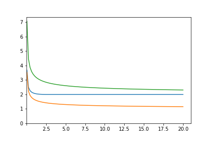
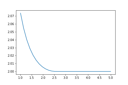
then there is such that for any fixed , with probability going to one. We will revisit this statement in context of the Erdős–Renyi graphs (see Corollary C below and Figure 2).
Futher, let us discuss the result at a more conceptual level. For a fixed , large enough and under the assumption , the –th largest eigenvalue is of order
A very similar formula has appeared multiple times in a different context — in the study of perturbed random matrices. The spectrum of random matrices perturbed by fixed matrices of a given structure has been subject of very active research. More specifically, consider the spectrum of , where is an Wigner matrix and is a fixed deterministic symmetric perturbation. When is of a finite (or relatively small) rank, the limiting spectral distribution of is not affected by the perturbation (remains semi-circular) due to the interlacing property of the eigenvalues. However, the perturbation can affect largest eigenvalues forcing some of them to get asymptotically detached from the rest of the spectrum. This phenomenon was first considered in [23] where the authors, motivated by estimating the largest eigenvalue of the adjacency matrix of an Erdős–Renyi graph, studied rank one deformations of a Wigner matrix. Later on, considerable interest in deformed random matrices was also connected with the work [4], where the famous BBP phase transition phenomenon was put forward. A large number of articles was devoted to investigating the phase transition in a variety of models as well as to studying fluctuations of the largest eigenvalues detached or not detached from the bulk [4, 12, 8, 9, 5, 14, 15, 16, 17, 22, 29, 30, 36, 39, 41, 42, 45, 48]. We refer, among others, to survey [40] for a review of the subject.
Theorem (BBP Phase Transition, see [40, Theorem 2.1]).
For each , let be an Wigner matrix whose entries on and above the main diagonal are independent copies of , where is centered variable of unit variance. Suppose further that has a finite fourth moment. Fix and , and for each , let be an deterministic symmetric matrix of rank with non-zero eigenvalues . Then for any ,
-
•
If , then ;
-
•
If , then ,
where denote the eigenvalues of .
Note that if in the above theorem was replaced with then the theorem would describe exactly the same asymptotic behavior as revealed in Theorem A. We can give the following non-rigorous justification for this similarity. Let us reconsider the matrix from Theorem A, and note that due to concentration inequalities, most of the rows have their norms squared concentrated around . Only a small fraction of these rows can have their norm far from . For simplicity, suppose that only one row of (say, the first one after an appropriate permutation) has the Euclidean norm significantly larger than . Then we may decompose our matrix as
where is obtained from by a regularization procedure of reducing the entries of the first row and column (the ones with the largest norms) in such a way that the Euclidean norm of the transformed row and column is equal , and is the remainder: the symmetric zero diagonal matrix whose first row/column’s Euclidean norm is equal to , and the matrix entries not in the first row or column of are zeros (here, we use “” instead of the equality sign to emphasize that our model describes the actual distribution of only approximately). In a sense, we treat the extra mass in the rows and columns of of large Euclidean norms as a deformation of the regularized matrix . We take this extra mass from the first row and column of and transfer it to the matrix which is perceived as a perturbation of . Clearly, is of rank with eigenvalues . On the other hand, by our assumption, all rows of have their norms concentrated around which could suggest that the spectrum of has no outliers. Now, Theorem A states that if , then has all its eigenvalues asymptotically bounded by ; whereas, if , then has an outlier and its value is given by . This parallels the BBP phase transition phenomenon. Let us emphasize once more that the above discussion is meant only to suggest similarities between the two models and is not developed rigirously. It seems interesting to understand if such a connection could be elaborated. We remark that there has been several works recently concerned with regularizations of random graphs/matrices i.e procedures designed to reduce the norm of random matrices by changing a few of its entries (see [21, 33, 44, 43]).
Another consequence of Theorem A is that the operator norm of the matrix has the same order of magnitude as . As previously stated, one has deterministically , and Theorem A implies that the reverse inequality is true up to a universal constant. Indeed, an analysis of the parameter shows that for any ,
with probability going to with . To view this, note that when , we have while otherwise . Moreover, in view of standard concentration inequalities, for any one has with probability going to one with . Therefore, Theorem A implies that for any , we have
| (1) |
with probability going to one with (see Corolllary C and Figure 1 for the case of the Erdős–Renyi graphs). This phenomenon was first observed by Seginer [47] who showed that for matrices with i.i.d entries, the operator norm is comparable, up to a constant, to the maximum Euclidean norm of its rows/columns. We note that Seginer’s result applies to a much wider class of distributions of the entries (as long as they are i.i.d) and while it is stated in [47] for expectations and for non-symmetric matrices, it is not difficult to obtain its extension to tail estimates for norms of symmetric matrices. Theorem A recovers Seginer’s observation in the setting of uniformly bounded entries and gives asymptotically optimal relation between the spectral norm and the maximum Euclidean norm of the rows. While one might be tempted to think that this comparison is valid for any random matrix with independent entries of different variances, Seginer [47] provided an example showing that it is not the case even for the class of inhomogeneous matrices with subgaussian entries. Nevertheless, it was shown in [32] that for inhomogeneous Gaussian matrices with independent Gaussian entries having arbitrary variances, the spectral norm is equivalent, up to constant multiples, to the maximum Euclidean norm of rows. We refer to [32] for further discussion and references concerning this phenomenon.
Theorem A deals with sparse matrices with centered entries and does not directly provide information on the magnitude of the largest eigenvalues in the non-centered setting. Assume is an symmetric matrix whose entries on and above the main diagonal are i.i.d copies of , where is a Bernoulli with probability of success and is a uniformly bounded real random variable of unit second moment (not necessarily centered) independent of . Naturally, one could recenter the matrix and consider the matrix in order to estimate . However, the centered matrix is no longer sparse and Theorem A cannot be applied. Moreover, standard symmetrization technique replacing with a difference of two independent copies of , would result in extra multiplicative constants. Indeed, one can write
where the matrix has entries of the form , with being independent copies of . This matrix is sparse and has centered entries so that Theorem A can be applied. However, the rows of have on average by larger Euclidean norms than rows of , resulting in an extra constant factor in the upper bound for obtained by this procedure. In order to capture the true asymptotic behavior of , we develop a special procedure relating the spectrum of the non-centered matrix to a specially chosen centered model. This reduction will be discussed in more detail in the next section. Let us state the second main result of this paper.
Theorem B.
Let be a uniformly bounded real random variable with . For each , let be an symmetric random matrix with i.i.d. entries above and on the main diagonal, with each entry equidistributed with the product , where is (Bernoulli) random variable independent of , with probability of success equal to . Assume further that with and . Then, defining as in Theorem A, i.e
for each fixed , the sequence converges to one in probability, where denotes the -th largest (by the absolute value) eigenvalue of .
Theorem B is obtained as a combination of Theorems 12.4 and 13.1 of the paper. The main application of Theorem B concerns the random Erdős–Renyi graphs , by taking to be constant . In [31], it is shown that the largest eigenvalue of almost surely satisfies
where tends to as tends to infinity, and is the degree of the -th vertex of . Of particular interest is the second eigenvalue as the difference may be viewed as a measure of the graph expansion properties. As stated previously, when , it is known that [23, 50, 7, 32]. With further constraints on , more precise information, including fluctuation intervals and limiting distribution of the extreme eigenvalues is available in the literature [19, 20, 34, 26, 27]. In contrast, when , it is shown in [6] that concentrates around the square root of the maximum degree in the graph (in the same paper, the authors study the -th largest eigenvalue, for arbitrary and ).
In the window , no asymptotically sharp results for were previously available. Moreover, it was not even known if there is a sparsity threshold (a multiplicative factor of ) where the phase transition between existence and absence of non-trivial outliers in the spertrum can be observed.
It follows from Theorem B that converges to in probability, where
The distribution of the maximum degree of the Erdős–Renyi graph is very well understood (see, for example, [11, Theorem 3.1]). This leads to an explicit formula for and thus an asymptotic formula for . The phase transition for the Erdős–Renyi graphs is considered in the following statement.
Corollary C (Outliers in the spectrum of the Erdős–Renyi graphs).
For each , let be the Erdős–Renyi random graph on vertices, with parameter . Assume that and . Let be the -th largest by absolute value eigenvalue of the adjacency matrix of . Then, denoting
for any the ratio converges to one in probability. In particular,
-
•
(No non-trivial outliers) If then for any , converges to in probability.
-
•
(Outliers) If then there is such that for any , we have
.
Here, denotes the main branch of the Lambert function defined by .
Shortly after this manuscript was posted on arXiv, related results appeared in the work [1]. In particular, the phase transition above happening at for the appearing of outliers in the spectrum of the Erdős–Renyi graphs was also captured in [1] and the results of [1] extend as well to the Wigner matrix model studied in this paper. The authors of [1] apply a completely different technique which cleverly exploits a tridiagonal representation of a hermitian matrix and a relation with the spectrum of the associated non-backtracking matrix. We refer to [1] for more details.
Acknowledgements
A part of this work was done while the second named author was visiting Georgia Tech in July 2018. He would like to thank the institution for the great working conditions. P.Y was supported by grant ANR-16-CE40-0024-01.
2. Overview of the proof
This section is intended to give a fairly detailed overview of the proofs of our main results, giving an emphasis to those parts of the argument which, in our opinion, may turn out useful in future works on the subject. As a starting point, we consider a simplified model that shows how (and why) the quantity defined in the main theorems, appears in the proof.
As it was mentioned in the introduction, it seems instructive to think of our model as of a standard (dense) Wigner matrix being perturbed by a small number of rows/columns of relatively large norms. These rows and columns distort the matrix spectrum and (if the magnitude of the norms exceeds a certain threshold) shift the largest eigenvalue to a non-classical location.
We will consider a simpler deterministic model as an illustration. Assume that the entries of our symmetric matrix take values and that the locations of non-zero elements are fixed (non-random), and that is the corresponding simple deterministic graph which does not contain any cycles. Assume further that the support length (i.e. the vertex degree) of every row/column, except for the first one, is at most , while the support of the first row/first column has length . We will estimate from above the norm of using the trace method. Fix . A standard formula gives
where the summation is taken over all closed paths of length on . For each vertex of the graph , and its neigborhood , we fix a bijective mapping from into the integer interval — a “local indexation” of neighbors of .
First, we consider the paths starting at vertex (of degree ). Each such path corresponds to a diagram on i.e. a mapping with and, for every , whenever is farther from vertex than , and otherwise. Note that the diagram is a Dyck path i.e. it is non-negative everywhere and is equal to zero at . To each moment of time with we can put in correspondence the local index . Then the data structure consisting of the diagram and the indices corresponding to times with , will uniquely identify the path, i.e. in order to estimate the number of paths it is sufficient to estimate the number of such data structures.
Note that whenever and , the corresponding index can only take values in , while in the case the index takes values in . For each , let be the total number of the Dyck paths of length with returns to zero (counting the point ). By a standard formula, . Thus, the total number of the data structures can be estimated by
(see Lemma 7.6 of this paper for a proof of the last relation).
We omit computations related to the setting when the starting vertex of a path is not ; the upper bound is essentially the same as above. Overall, assuming an appropriate growth condition for (in particular, ), we can show that
Taking into account that , the last expression in the brackets perfectly agrees with the definition of in the theorems from the introduction.
Proving that the above model accurately describes the situation in case of sparse Wigner matrices is the main technical problem within the proof. More specifically, we need to show that the norm of a typical realization of a sparse Wigner matrix with uniformly bounded entries is essentially determined by local tree-like structures similar to the one in the above example. In order to implement this strategy, we need to resolve a number of issues; among them:
-
•
Show that the contribution of paths with cycles is not much larger than the contribution of paths on trees.
-
•
Deal with the fact that there are multiple vertices of large degrees within the graph, and rather than taking two distinct values the degrees are “continuously” distributed within some integer interval.
-
•
Develop a procedure to condition on a “good” realization of the matrix and the underlying graph . Clearly, in the sparsity regime we study, taking the unconditional expectation of would result in highly suboptimal bound on the norm. While taking a conditional expectation given a “good” realization of the graph and of absolute values of the matrix entries may seem a reasonable strategy when the entries are symmetrically distributed, in the case of non-symmetric distributions a different approach has to be used.
-
•
Transfer the results obtained for centered matrices to the non-centered setting, in particular, the adjacency matrices of the Erdős–Renyi graphs. Since the centered adjacency matrices are no longer sparse, this problem requires a special symmetrization procedure.
-
•
Show that the upper bound obtained using this strategy is optimal i.e. prove a matching lower bound.
As a common starting point, given an symmetric matrix , we write
where the sum is taken over all closed paths of length on the complete graph , the product — over all edges in (counting multiplicities), and where is the matrix entry corresponding to the edge . While an averaging argument (taking the expectation of the expressions on the left and right of the above relation) is a usual step in classical applications of the trace method, in this paper we rely on computing the expectations only when considering paths with many edges of multiplicity one, whereas for other paths we estimate the products for every realization of the matrix within some special event of probability close to one.
Data structure. Classical applications of the trace method often involve defining an auxiliary structure associated with a path, which simplifies counting; for example, diagrams and auxiliary sets marking cyclic elements within the path. In our proof, the data structure associated with a path plays a fundamental role, and, in addition to “usual” information (times of discovering new vertices/edges, traveling directions along a previously discovered edge) also contains data about the magnitude of the Euclidean norm and the distribution of mass across the rows/columns corresponding to the graph vertices.
At an abstract level, our approach can be described as follows: we define an injective mapping from the set of paths into a “data space” , and for each element we define a weight in such a way that for all paths. Then, in view of the injectivity,
This way, analysis of the paths can be completely replaced by counting on the data space. A crucial part of this approach is to define the mapping and the data space in such a way that, on the one hand, is sufficiently “rich” and both and are simply structured so that injectivity can be easily established and the sum on the right hand side — (relatively) easily computed; on the other hand, is not too large so that the sum can be efficiently controlled from above. A formal definition of our mapping and the proof of injectivity is given in Section 4; some structural properties of the data space are discussed in Section 5. A satisfactory definition of the weight presents an issue on its own. As we attempt to make counting over the data structures simpler than counting over the paths, we inevitably lose information about the matrix when transfering the problem to the space ; in particular, we do not have in possession the precise information about the value of the product of the matrix entries corresponding to a given data structure. In order to deal with this issue, we introduce vector majorizers.
Vector majorizers. A majorizer of a vector in is any vector such that coordinate-wise, i.e. for all , where denotes the non-increasing rearrangement of the vector of absolute values of components of . The crucial observation, which we make in a rather general deterministic setting in Section 3.2 and in the more specific probabilistic setting in Section 9.1, is that there exists a small collection of majorizers such that for any typical realization of our matrix , every row can be majorized by a vector from this collection having only slightly larger norm. Now, in order to implement the weight function on our data space , it is sufficient to record in each structure which majorizers from have to be used, and then define by analogy with the weight of a path, replacing entries with corresponding components of majorizers.
Let us provide a simple example to illustrate the idea. Assume that , and that contains two vectors — and . Assume that a typical realization of our matrix is
| 0 | 1 | -0.8 | 0 |
| 1 | 0 | 0.6 | 0.5 |
| -0.8 | 0.6 | 0 | 0.3 |
| 0 | 0.5 | 0.3 | 0 |
Then we can assign to rows and the majorizer , and to rows and — majorizer . Consider a path of length . Obviously, the absolute value of the path weight is . We can interpret this product as “the second largest component of first row squared times the second largest component of the second row squared”. Now, replace the rows with corresponding majorizers. We get “the second largest component of majorizer squared times the second largest component of majorizer squared”, i.e. . This is the weight of the data structure .
Let us note that in the actual proof, it will be more convenient for us to define majorizers for vectors of squares of the matrix entries, i.e. vectors of the form ; otherwise, our approach is very similar to the above example. Since the number of majorizers is much smaller than the space of possible realizations of the matrix rows, adding the information about the majorizers does not increase the data space by too much, and a satisfactory upper bound for is possible. In fact, standard concentration inequalities imply that with very large probability a vast majority of the matrix rows can be efficiently majorized by a single vector which we call a standard majorizer. For those rows, no additional information should be added to the data structure which further controls the complexity of the space .
Paths with many edges of multiplicity one. In classical applications of the trace method, paths having edges of multiplicity one do not participate in the counting process since the expectation of the corresponding path weight is zero. As we already mentioned above, in our setting taking the unconditional expectation of the trace cannot give a satisfactory upper bound whereas conditioning on a “good” event (say, matrix realizations with predefined statistics of norms of their rows and columns) produces complex dependencies within the matrix, and computation of the conditional expectation becomes challenging. For paths with relatively few edges of multiplicity one, instead of the averaging, we compute an upper bound for the sum of path weights valid everywhere inside the “good” event, by bounding (the absolute value of) every path weight by the data structure weight, followed by some computations which rely on the structure of the data space (see discussion above). However, this approach is not applicable for paths having many edges of multiplicity one. For a typical realization of our matrix, the path weights of such paths are split into approximately equal parts according to their sign, and multiple cancellations occur. Bounding each path weight individually by its absolute value destroys these cancellations and cannot produce a satisfactory estimate. The approach we take is to track these cancellations while conditioning on a “good” realization of the matrix, even though this conditioning produces dependencies across the matrix. Our method provides satisfactory estimates only for paths having relatively many multiplicity one edges, and thus complements the argument based on the data structures. The structure of the event we are conditioning on plays a crucial role. The formal description of the method is given in Section 10. Here, we would like to give a geometric viewpoint to it. Let be our symmetric random matrix, and let be the corresponding random graph on (whose edges mark non-zero entries of ). Assume that we need to compute the conditional expectation of a product given the event
where is an appropriately chosen parameter. Geometrically, the event defines a bounded set within the linear space of symmetric matrices , and the conditional expectation of can be viewed as integration of over with respect to an appropriate measure. It turns out that neighborhoods of points within located far from the boundary , contain approximately equal mass of positive and negative realizations of , and a cancellation within the integral can be verified. More precisely, we can show that if the number of surfaces , which are close to our chosen point, is not very large then necessarily a neighborhood of this point is “well balanced” in terms of the values of . Thus, the parts of in which cancellation does not happen are located close to the “corners” of , and their measure is very small if the number of multiplicity one edges in is large. Therefore, the conditional expectation of given is very close to zero.
Non-centered matrices. Let us discuss here how to get an asymptotically sharp upper estimate for () for a sequence of non-centered matrices , with the help of Theorem A for sparse centered matrices. As it was already mentioned in the introduction, standard centralization procedures — replacing with or with the difference of two independent copies of — do not allow to reduce the problem of bounding the eigenvalues of a non-centered sparse matrix to the setting of Theorem A. Indeed, in the first case we would obtain a non-sparse random matrix whereas the second approach indroduces a suboptimal constant factor in the final estimate. To deal with this issue, we carry out a different symmetrization procedure designed specially for sparse matrices. To avoid technical details in this overview, we describe a model different at certain points from the one we actually use but easier to discuss informally.
Assume that is a sparse Bernoulli matrix (i.e. the adjacency matrix of the Erdős–Renyi graph; we can assume for simplicity that loops are allowed) and let be the success probability of each entry. Fix a small constant and consider another Bernoulli random matrix with the entries having probability of success . Then the difference is a centered (and still sparse) random matrix, and we could apply Theorem A to get an upper bound on its largest eigenvalue. Note that the sparsity parameter of the matrix is , whereas the variance of each entry is . Therefore, to apply Theorem A we should rescale the matrix by the factor (approximately) . We get that for large enough , with large probability
Our next observation is that the maximal norm of the rows of is typically much smaller than the maximal norm of the rows of . As an informal justification, we can point to the trivial relation , . This allows us to replace with in the last display formula, so that, after cancelling , we obtain
As the last step, we observe that , where is a relatively small perturbation of the matrix , and cannot significantly decrease the spectral norm. The way it is actually done in our proof is to consider a random unit vector measurable with respect to and such that everywhere on the probability space. Then, using our assumption that is small and that and are independent, it is possible to show that is small with probability tending to one, implying that
Combining this relation with the previous formula, and letting , we obtain an asymptotically sharp upper bound for .
Lower bound for the –th largest eigenvalue. As the last element of the proof, we discuss the lower bound for the largest eigenvalues. Unlike the upper bound, this part of the argument does not use the trace representation, and instead is based on a mixture of combinatorial arguments (which give us necessary structural information on the underlying graph) and “geometric” methods which use an explicit construction of a random vector capturing the values of the leading eigenvalues. For the sake of simplicity, we will only discuss the bound for the operator norm; an estimate of for is obtained by decomposing the matrix into blocks and carrying out the argument sketched below on each of the blocks.
We recall that the basic test case in the study of the upper bound is a tree of finite (but large) depth rooted at the vertex corresponding to the row/column with the largest Euclidean norm. In a sense, the whole proof of the upper bound can be viewed as a justification of the fact that this test case presents a significant contribution into the sum-of-paths representation of the trace. For the lower bound, we take the same tree in the underlying random graph but this time we construct a special random vector (modelled in accordance with the tree structure) such that is close to the spectral norm of .
Let be a matrix with the entries taking values in , and let be the graph on with the edge set corresponding to non-zero entries of . We will further assume that the vertex of having the largest degree is , and that the –neighborhood of in (for a large constant ) is a tree whose nodes, except for the root and the leaves, have a degree . Our assumption that the neighborhood is a tree, is reasonable in view of the sparsity of our model (we avoid going into technical details here). For any integer , we let be the set of all vertices of the tree having depth (so that, in particular, ). We then define our vector as
where for each , we set
, , are some parameters and is the canonical basis in . The vectors have disjoint supports, and thus can be viewed as a weighted combination of tree nodes of odd depth; with the weight shared by all nodes (basis vectors) of depth . The latter condition is reasonable as the nodes of the tree having the same depth are indistinguishable when unlabelled. The condition that we take only even values of is not crucial; at the same time any given matrix row is supported on vertices which either all have odd depth or all have even depth, and this produces a recursive relation between and in the computations making the separation of odd and even tree layers somewhat natural.
The formula for the vector was obtained by trial and error although the above remarks suggest that the choice of such structure is quite natural. The values of the parameters which produce maximal (or close to maximal) value of can be easily deduced; in fact, we take as a geometric series determined by and the degree of vertex (we refer to the proof of Lemma 13.6 for details).
3. Preliminaries
Given two integers , we denote by the corresponding integer interval. For the interval on the real line with the same boundary points, we will use notation .
Let be an undirected (simple) graph. Given vertices and in , the edge connecting and is denoted by . A path of length on is a sequence of vertices of where each pair of successive vertices forms an edge in . We allow the vertices in the path to repeat. A path is closed if the first and last vertex of the sequence coincide. It will be convenient for us to view a path on the graph as a mapping from an integer interval to the set of vertices . If is a path on then are vertices travelled by . For any , by we denote the subpath .
For any connected graph there is a natural metric on its set of vertices induced by the graph distance i.e. for every , is the length of the shortest path in starting at and ending in . For any , the -neighborhood of a vertex is the subgraph of obtained by removing vertices with distance more than to . The diameter of is the largest distance between any pair of its vertices. Further, a subset is –separated if for any two distinct elements of . We say that is a maximal –separated subset of if it is –separated and there is no vertex whose distance to is strictly greater than . Everywhere in the text below, the terms “distance”, “diameter”, “-neighborhood” and “-separated set” are used in the above sense.
Given an edge of , we denote by the set of two vertices incident to i.e. if then . Further, for any we define . Conversely, given a subset , by we denote the collection of all edges of which are incident to some vertex in . We say that is a cycle edge of if it belongs to a cycle within ; otherwise we say that is a non-cycle edge. We say that a graph is -tangle free if every neighborhood of radius in has at most one cycle.
The next lemma provides a standard upper bound on the number of -separated points in a connected graph.
Lemma 3.1.
Let be a connected graph containing vertices which are -separated. Then .
It is a standard fact that any connected graph admits a subgraph with the same vertex set and without cycles (a spanning tree). We will need a relative of that property which tells us that we can delete half of cycle edges from a certain prescribed collection without destroying connectivity.
Lemma 3.2.
Let be a connected graph and be a connected subgraph of . Further, let be a collection of cycle edges of not contained in but incident to . Then there exists of cardinality at least such that the graph obtained from by removing edges from is still connected.
Proof.
Let be a subset of of maximal cardinality such that removing the edges in keeps the graph connected, and assume that . For every edge , let be the endpoint of not contained in (note that such vertex exists by the connectivity of and the maximal property of ). Take any edge . We will show that there exists a path on starting at , ending at a vertex in and not passing through edges in .
Indeed, if then there is nothing to show. Otherwise, since is a cycle edge, there is a cycle in containing . Let be the trail on starting at , ending at , and not passing through . Denote by the first time when (such time always exists since the path ends in ). Observe that if belonged to then we would obtain a path on from to not passing through , which contradicts the maximality of (since the removal of would keep the graph connected). Hence, , and cannot contain any edges from since otherwise one of its vertices would belong to . It remains to set to obtain a path starting at , ending at a vertex in and not passing through edges in .
Since , we have and by the pigeonhole principle, there are edges such that the corresponding paths; and , end at the same vertex . Concatenating these two paths, get that and are connected through a path on the edges in . Therefore, one of the edges or could be removed without destroying connectivity of the graph. Since both of these edges do not belong to , this contradicts the maximality of and we deduce that . ∎
As a consequence of the last lemma, we can bound from above the number of cycle edges of an -tangle free graph which are incident to a connected subgraph of small size.
Lemma 3.3.
Let be a connected -tangle free graph, be a connected subgraph of with , and be the collection of all cycle edges of incident to but not contained in . Then .
Proof.
Let be the set obtained from Lemma 3.2 and let be the (connected) subgraph of with the same vertex set and with the edge set . Let be a maximal –separated net in and note that, by Lemma 3.1, we have . For each vertex , let be such that .
Assume first that . Then, by the pigeonhole principle, there are at least couples of vertices with , and . This implies that and can be connected by a path in of length at most , and similarly for and . At the same time, and can be connected by a path on , and similarly for and . Therefore, there are at least two distinct cycles in of length at most , and with distance between the two cycles at most . Hence, there is a vertex in such that its -neighborhood contains at least cycles, which contradicts the -tangle free property of by our restriction on .
Thus, we deduce that . Further, for any , there are at most two edges in incident to it, as otherwise we would get at least two cycles in of length at most in the neighborhood of contradicting the -tangle free property of . Finally, observe that there is at most one edge in with both end points in , as otherwise we would get cycles of lengths at most at distance at most from one another, leading to a contradiction as before.
Hence, we get . Combining this with the bound from Lemma 3.2 and the one on the cardinality of , we complete the proof. ∎
3.1. Edge and vertex discovery, and statistics of special vertex types
Let be an undirected graph. As we mentioned above, it will be convenient to see a path on of length as a function where for every , indicates the vertex reached by the path at the step (“time”) . For each path on , we denote by the undirected subgraph of obtained by deleting the edges and vertices not visited by .
Let be the set of times such that is a cycle edge of travelled either once or at least three times by . Now, for any cycle edge in , the discovery time of is the smallest such that
Note that the discovery time for a cycle edge of the graph may be different from the first time the edge is traveled by the path.
In this subsection, we discuss three types of special vertices of the graph : cycle meeting points, splitting points and cycle completion points. The main purpose is to show that under the assumption that is -tangle free (for a large enough ), the total number of the special vertices is very small.
Let be some path on (we change notation here as may serve both as the path or as its sub-path). For every , we define the direction of uncovering of in as the direction in which it first appeared in the i.e.
The time of uncovering for is the smallest such that is an edge of . We once again would like to turn the Reader’s attention to the distinction between times of discovery and uncovering of a cycle edge in the graph.
Let be a vertex of .
-
•
is cycle meeting point of if there are at least three distinct vertices of such that , and are cycle edges of .
-
•
is a splitting point of if there exist vertices such that , are cycle edges in and and .
-
•
is a cycle completion point if there is time such that and the number of cycles in is strictly less than the number of cycles in .
All vertices of which belong to one of the above types, will go under the name special cycle vertices of . Note that a given vertex can be simultaneously of more than one of the above types. Next, we define the concept of discovery times for the special cycle vertices. The discovery time of a special cycle vertex of is the smallest such that is a special cycle vertex of . Notice that the discovery time of a special cycle vertex is not equal to the first time the path visits this vertex.
As a simple corollary of Lemma 3.3, we get the following statement which bounds the number of cycle edges incident to a cycle meeting point.
Corollary 3.4.
Assume that is -tangle free with , and let be a cycle meeting point in . Then the total number of cycle edges of incident to does not exceed .
In the next lemma, we bound the total number of the cycle meeting points.
Lemma 3.5.
Assume that the graph is -tangle free, with . Then the total number of cycle meeting points in is at most for some universal constant .
Proof.
Let be the number of cycle meeting points in . We will assume that (otherwise, there is nothing to prove). Denote by a maximal -separated net in and note that by Lemma 3.1, we have . Clearly, there exists a vertex such that its -neighborhood contains at least cycle meeting points.
Let be a spanning tree for , and denote by a subtree of obtained by successively removing edges incident to degree one vertices which are not cycle meeting points of (and then throwing away the obtained isolated vertices). Note that this operation will necessarily keep all cycle meeting points which fall into , inside as any two such vertices are connected by a path within , whose edges cannot be removed. In particular, is non-empty. Note also that all leaves of are by construction the cycle meeting points of .
Let be the set of all cycle edges of which are incident to vertices in but not contained in . Note that, by the definition of a cycle meeting point, for any leaf of , there are at least edges from incident to it. Further, for any cycle meeting point which is a node of degree in , there is at least one edge from incident to it. Finally, it is easy to check that the number of nodes of degree at least in any tree is less than the number of its leaves. Since any edge in is incident to at most cycle meeting points in , the above observations imply that
Applying Lemma 3.3 with (note that ), we get that
whence for some appropriate constant . ∎
In order to bound the number of splitting and cycle completion points, it will be convenient to introduce a notion of a cycle interval. By a cycle interval in we understand an (unordered) collection of distinct cycle edges in of the form , where none of the vertices are cycle meeting points of and, if , then and are cycle meeting points of . Note that with this definition, every cycle edge of belongs to a unique cycle interval, and no two distinct cycle intervals share more than common vertices. Furthermore, any cycle interval belongs to one of the following two types:
-
•
Either is a full cycle of which has at most one common vertex with other cycles of ,
-
•
Or is a collection of consecutive edges of some cycle in which is bounded from both sides by two distinct cycle meeting points.
In the next lemma, we give an upper bound on the number of cycle intervals.
Lemma 3.6.
Assume that the graph is -tangle free, with . Then the number of cycle intervals in is at most for some universal constant .
Proof.
The definition of a cycle interval implies that each interval in is either a full cycle of or has cycle meeting points as its boundary vertices. In view of Lemma 3.5 and Corollary 3.4, the number of intervals of the second type is bounded above by for some constant . To count the number of intervals in which are full cycles, note that since the graph is -tangle free, the number of cycles of of length at most is at most . Indeed, this can be verified by constructing an -separated set in consisting of “representative” vertices which belong to distincs short cycles, and then applying Lemma 3.1. Finally, it remains to note that the number of disjoint cycles of length greater than is at most . ∎
Lemma 3.7.
Let be a cycle interval in . Then, among the vertices , there is at most one splitting point.
Moreover, if is -tangle free, then the total number of splitting points in is at most , for some universal constant .
Proof.
Assume that the cycle interval contains distinct splitting points in its interior, say, for some . Assume further that the point is visited for the first time by earlier than . The vertex cannot be reached for the first time by through any of the edges or since this would violate their uncovering directions. But then must be accessed through another edge which necessarily would become a cycle edge of . But then is a cycle meeting point – contradiction. Thus, each cycle interval contains at most one splitting point in its interior.
To prove the second part of the lemma, note that the number of splitting points is at most three times the number of cycle intervals in (if we count , as possible splitting points in ), and Lemma 3.6 implies the estimate. ∎
Lemma 3.8.
Let be -tangle free. Then the total number of cycle completion points of is bounded above by for some universal constant .
Proof.
Note that each cycle interval may contain at most cycle completion point in its interior. The result follows by applying Lemma 3.6. ∎
3.2. Majorizers
Given a vector in , let be the non-increasing rearrangement of the absolute values of coordinates of . Further, given a non-increasing vector , we say that is a majorizer for , and write , if for all .
We will consider a collection of majorizers for a special class of vectors. Given and , define the set of all –dimensional vectors , such that , , and has at most non-zero coordinates. We have the following lemma:
Lemma 3.9.
For , and satisfying and , there exists a subset of cardinality at most such that for every there exists which is a majorizer for , and, moreover, . Here, is a universal constant.
Proof.
For any vector , we write
where has at most non-zero coordinates all of which are smaller than while has all its non-zero coordinates lying between and . Note that the rearranged vector having non-zero coordinates all of which are equal to is a majorizer for for any . Moreover . Therefore, our task is to construct a majorizer for any given such that , then take which is a majorizer of satisfying .
Having in mind the above reduction procedure, we may therefore consider the set of all –dimensional vectors , such that , , has at most non-zero coordinates, and each non-zero coordinate is at least . We now construct a majorizer for any given vector and verify that it satisfies the required properties. Define ,
where is a universal constant which will be determined later. Further, for every we let
and, finally, define the –dimensional vector by
It is not difficult to see that , just by our construction. Next, we estimate the –norm of . Observe that the –dimensional vector satisfies (this can be easily checked, say, by embedding into ). Further, by our construction, assuming that the constant is sufficiently small (and is sufficiently large), we have
implying , so that
Hence, the vector is a majorizer for . This gives
Let be the set of all vectors satisfying the following conditions:
-
•
;
-
•
;
-
•
;
-
•
is constant on and on , .
It is immediate that the vector constructed above belongs to . Thus, to finish the proof, it remains to estimate the cardinality of . Observe that coordinates of any vector from may take at most different values, and for any such that , we necessarily have that is zero on (as otherwise the assumption on its –norm will be violated). Thus, there are at most “non-trivial” levels of , whence
for an appropriate constant . The result follows. ∎
4. Mapping to a data structure
Given an symmetric matrix with zero diagonal, we denote by the graph with the edge set . With some abuse of terminology, we will say that a vertex of is majorized by a vector if the non-increasing rearrangement of the sequence is majorized (coordinate-wise) by . Given a vector , we say that a vertex of the graph is –heavy if it is not majorized by .
Let be a large natural number, and , , satisfying
| (2) |
Define
| (3) |
as the set of all symmetric matrices with zero diagonal satisfying the following conditions:
-
•
For any , .
-
•
is -tangle free.
-
•
Each non zero entry of satisfies .
-
•
All non-zero entries of are distinct (up to the symmetry constraint).
-
•
For any , .
-
•
For any vertex , the number of its –heavy neighbors is at most .
Following the previous section, define the discrete set
where is taken from Lemma 3.9. Note that, by the lemma and since , we have
| (4) |
for a universal constant , and for any vector there is with and .
Define a mapping which will assign to every element of a majorizer from . We will call the standard classifier.
Let , and denote by its associate graph . We are interested in estimating the quantity
| (5) |
where the sum is over all closed paths of length on , the complete graph on vertices. Note that any having an edge not in do not contribute to the above sum, and we are therefore left with paths on . To this aim, we will associate to each path a data structure which would help us encode the path and its contribution to the above quantity. Everywhere below, is a path on . We start by associating a diagram to this path, where by a diagram on an integer interval we understand a function such that for all . The graph of consists of a sequence of “diagonal up arrows” and “diagonal down arrows” connecting the neighboring points and (“up arrow” if or “down arrow” if ). In the sequel, we will write (resp. ) to indicate a diagonal up (resp. down) arrow between the points and .
With each closed path on of length , we associate a diagram which can be iteratively constructed as follows. First we set and for every ,
-
•
If was not traveled before time then we set ;
-
•
If is a non-cycle edge of which was traveled before time , and the first time it was traveled in direction , then we set ;
-
•
If is a non-cycle edge of which was traveled before time , and the first time it was traveled in direction , then we set ;
-
•
If is a cycle edge of which was traveled before time (in any direction) then we set ;
Note that the value of at is not necessarily zero: in general, the number of up-arrows and down-arrows do not agree. However, we have
Lemma 4.1.
Let be a closed path on of length . Then for every non-cycle edge of , the number of up arrows in corresponding to is equal to the number of down arrows for .
Proof.
Let be a non-cycle edge of . Since is closed, this condition implies, in particular, that is traveled an even number of times, with each of the two possible directions traveled the same number of times. Then the algorithm of constructing implies the desired conclusion for . ∎
The diagram above will give us partial information on whether we are discovering a new edge, or re-traversing it, as well as it’s uncovering direction. To further encode where the path is heading at each step, we will be introducing local indexation of vertices. We will use three types of indexation.
Given a vertex and its neighbor in , the simple local index of with respect to is the position of in the sequence of all neighbors of ordered according to the magnitude of ; formally
Further, for every vertex , define as the set of all –heavy neighbors of (as defined at the beginning of the section). Then the heavy-vertex local index of is the position of in the sequence of elements of arranged in the order determined by the magnitude of :
Unlike the first two, the third type of local indexation depends on . Let and let
| (6) |
The cycle local index of a vertex is defined by analogy with the above types of indexation and utilizes the same ordering:
Note that the cycle local index of a vertex depends on time and can vary for different . We record the following simple lemma (which is a consequence of the estimates from Section 3.1) for future reference:
Lemma 4.2.
Assuming that (in particular, is -tangle free for some ) we have for any closed path on of length and any time :
where is a universal constant.
For each closed path on , we define a data structure consisting of
-
•
The diagram ;
-
•
The initial vertex ;
-
•
Sets of times and ;
-
•
A weight function ;
-
•
A vector-valued mapping .
The data structure is rather complex, and before giving a formal definition of its components let us briefly describe their purpose. The diagram gives partial information on times when a new edge is discovered as well as direction in which an edge is traveled at a given time. The set will be used to store information about special cycle vertices associated with the path. Further, will encode information about the cycle edges of having multiplicity either one or at least three: there are several (technical) reasons for treating the cycle edges of multiplicity two differently. The set stores data about –heavy vertices; roughly speaking, about the rows and columns of which have a big support, or a big –norm, or an “unusual” profile. The weight function will store an index of a currently traveled edge. The type of indexation used will depend, in particular, on the type of the vertex/edge.
Now, we turn to the formal description. Construction of the diagram was discussed above. The initial vertex is simply the vertex in .
Definition of . We set
Definition of . For each , we add to the set if one of the two conditions is satisfied:
-
•
If is a special cycle vertex of with discovery time at most and there is down arrow from to in the diagram , or
-
•
is a special cycle vertex of with discovery time at most and there is an up arrow from to in the diagram.
Definition of . For any , we add to the collection if the vertex is –heavy.
Definition of the weight function. The weight function is constructed as follows:
-
•
If “ and is a cycle edge of with discovery time at most ”
or
“ is a special cycle vertex of with discovery time at most ”,
then is equal to .
-
•
Otherwise, if and is either a non-cycle edge or a cycle edge of with discovery time at least , then is equal to .
-
•
Otherwise, if and there is an up arrow from to , then is equal to , where the heavy-vertex local indexation is taken in .
-
•
Otherwise, if there is an up arrow (resp. down arrow) from to , then (resp. ), where the simple local indexation is taken in .
Note that the weight function is negative when the cycle indexation is used. The purpose of this convention is to make sure that we can see that the local cycle indexation is applied simply by looking at the value of , regardless of the structure of . This will be important below when discussing injectivity of our mapping.
It will be convenient to define
Note that with this definition
i.e. we interpret the initial time, if the starting vertex is –heavy, as an “up-time”. We will use similar notations , for subsets of , although in that case the definition is simpler since the zero time can never be included in :
We define by analogy the sets .
Definition of . First, define an auxiliary set
| (7) |
For a given , let be the non-increasing rearrangement of the vector . Then we take as the value of the standard classifier (defined at the beginning of this section). Thus, the mapping will instruct us which majorizer we should take for a given heavy vertex. The fact that is not defined on the entire set does not lead to a loss of information because of our choice of the definition for ; in fact, given values of on , it is possible to deduce the values of for all heavy vertices (see Proposition 5.4).
The reason why the mapping is defined on rather than on the entire set is that the latter would significantly increase the complexity of our data space, making it “too large” to allow a satisfactory upper estimate for sums of the data weights (we also refer to discussion in Section 2). Specifically, the set may have cardinality comparable to meaning that there are distinct mappings from admissible realizations of into the net of majorizers . The data space defined in this manner would have cardinality much larger than , which is unacceptable. On the contrary, such a problem does not exist for the set (which may also have cardinality of order ) since the increased complexity of large is overcompensated by the decreased complexity of the weight function (which has a much smaller range on points from , compared to “regular” vertices). Finally, it can (and will) be shown that the cardinality of the set can be bounded in terms of , , , allowing an efficient control of the size of the data space.
The data structure associated to a path will be written as , or, in the “reduced” form, (we remark here that will be used to count weights of paths, and is not employed for the rest of this section).
The data structures will be used to estimate the number of distinct paths on the graph as well as their contribution to (5). To set up the relation between paths and data structures, we will prove that the mapping is injective. For brevity, for the rest of the section we omit the subscript “” for elements of the structure. We start with an auxiliary lemma.
Lemma 4.3.
Let and be two paths mapped to the same structure , and let . Assume additionally that . Then
with the sets defined by (6).
Proof.
Since , any cycle edge of with discovery time at most is also a cycle edge of with the same discovery time. Similarly, every special cycle vertex of with discovery time at most must be a special cycle vertex of with the same discovery time. The result follows. ∎
Proposition 4.4.
The mapping constructed above is injective.
Proof.
Denote by the mapping of paths to data structures. Let be a data structure in the range of and suppose there are two paths and such that . Our goal is to show that for any , we have . We will prove the assertion by induction.
Clearly . Now, let and suppose that for any . We will verify that , by considering several cases which mirror the definition of the weight function . First of all, we need to make sure that the four cases in the definition of are matched for both paths. For a path , we say that
-
•
Condition (A) holds if either “ and is a cycle edge of with discovery time at most ” or “ is a special cycle vertex in with discovery time at most ”;
-
•
Condition (B) holds if (A) does not hold and and is either a non-cycle edge or a cycle edge of with discovery time at least ;
-
•
Condition (C) holds if (A)–(B) do not hold and and there is an up arrow from to in ;
-
•
Condition (D) holds if (A)–(B)–(C) do not hold.
We then have that condition (A) (respectively, B, C or D) holds for if and only if the same condition holds for . Indeed, by our convention, (A) holds if and only if the value of the weight function at time is negative, and (B) holds if and only if the weight function is zero; similarly, the conditions (C) and (D) are “path–independent” i.e. are determined completely by the data structure. Having this in mind, we now consider in detail each of the four conditions.
-
(A)
By the definition of , in this case . In view of Lemma 4.3, we have , and so matching cycle local indices imply that the corresponding vertices coincide: .
-
(B)
In this case, is equal to . Note that the definition of the set implies that there is a down arrow from to in the diagram , whence the edge is traveled before the time , and for some . Similarly, for some . However, there exists at most one vertex such that and is a non-cycle edge in , and similarly for . Since , we get , that is, .
-
(C)
Here, . Since the heavy vertex local indexation is independent of a path, this immediately implies .
-
(D)
If there is an up arrow from to in the diagram, then the path-independent simple local indexation is used, so necessarily . Finally, assume that there is a down arrow from to , and . It follows from the definition of that cannot be a special cycle vertex in (and in ) with discovery time or less. Further, it is clear that the edge exists in the graph , and similarly for . Let us assume that , and show that this leads to contradiction. To emphasize that the paths coincide up to time , we will use notation for , and instead of or whenever . We have three subcases.
-
(i)
Assume that is a cycle edge of with a discovery time at most , and that, similarly, is a cycle edge of with a discovery time at most . Note that if and then is a splitting point of , which is impossible. Similarly, if and then is a cycle completion point in , again leading to contradiction. Thus, we can assume that and . Let be the time such that the edge is uncovered by at ; and define time for the edge by analogy. We must have since otherwise would necessarily be a cycle completion point in . It is also clear that . Let be the smallest time such that . Now, if we assume that the edge is distinct from both and then becomes a cycle meeting point in , which is impossible. Hence, must be equal to one of the two edges. But then this (cycle) edge would be traveled by corresponding path at least three times: (resp., for ), and , contradicting the condition (because we are not in situation A). Thus, we showed that the situation when both and are cycle edges of (resp., ) with discovery times at most , is impossible.
-
(ii)
Assume that is either a non-cycle edge of or a cycle edge with a discovery time at least , and that the same holds for . We cannot have simultaneously and since this would imply that at least one of the edges is a cycle edge in . Hence, we can assume that . But then traveling from to should correspond to an up-arrow in the diagram, and we arrive at contradiction.
-
(iii)
In the last scenario, we assume that is either a non-cycle edge of or a cycle edge with a discovery time at least , but is a cycle edge of with discovery time at most . Clearly, we must have as otherwise we would get an up-arrow in the diagram (we also recall that the edge must be uncovered by the time ). Since is not a cycle edge of , then necessarily the uncovering of must happen after the uncovering of . Now since is not a cycle completion point, we must have . Since (otherwise, we would have been in situation A), then is only traversed twice by the time : at the moment of its uncovering and on the time interval . Since there is a path connecting to after the uncovering of then necessarily is a cycle completion point of , leading to contradiction.
-
(i)
∎
5. Properties of the data structure associated with a path
As in the second part of the previous section, in this section we omit the subscript “” for elements of the data structure corresponding to a path . In this part of the paper, we will establish some properties of the data structure defined in the previous section by identifying constraints on the sets and . First, the number of elements of corresponding to up arrows in the diagram cannot be much smaller than the number of elements in corresponding to down arrows:
Proposition 5.1.
Let be a closed path on an -tangle free graph (), and let and be the associated sets and diagram from the data structure. Then for some universal constant .
Proof.
Recall that a time is added to only if is a special cycle vertex of with discovery time at most . Denote by the set of all cycle meeting points, splitting points and cycle completion points in . Then, by combining Lemmas 3.5, 3.7 and 3.8, we get that the cardinality of is bounded above by for some universal constant . Let be the set of all distinct cycle edges of such that there is with . By Corollary 3.4, there are at most cycle edges incident to a given point in , whence the total number of distinct edges in is at most . For any such edge , we have
since automatically implies that is a cycle edge of multiplicity and only it’s second appearance is recorded with a down arrow. Therefore, we deduce that
Next, for any vertex , let to be the set of all times such that and is a non-cycle edge of . Note that the set of non-cycle edges of incident to must be traveled in alternating directions (towards , then from , etc.). Then necessarily
Therefore, we get
Combining the above estimates, we get the result.
∎
In the next proposition, we show that within time intervals not containing any elements of and such that the corresponding part of the diagram attains its minima at the interval endpoints, these endpoints correspond to the same vertex of the graph.
Proposition 5.2.
Let , be as before, and let be the corresponding set from the data structure for . Let and assume that, first, ; second, ; third, for all . Then . In particular, either both belong to or .
Proof.
We will show that ; then the second assertion of the proposition will follow automatically. In turn, to verify this property, it is sufficient to show that whenever are such that and and then necessarily . Indeed, an inductive argument based on the latter property will lead to the result.
Assume the opposite i.e. and denote , and . Since , then the edge appears previously in the path. Let be the time the edge was uncovered. We will consider several cases:
-
(a)
Suppose . We have either or . Since then the edge wasn’t uncovered before the time . Therefore, is connected to through a path in which doesn’t contain the edge . Hence, a new cycle is formed at time , making a cycle completion point. But then, by the definition of , the time must belong to which contradicts the hypothesis .
-
(b)
Suppose and that . Therefore and , and is necessarily a cycle edge (of multiplicity ) in . Let be the first time when a cycle containing the edge is completed. Clearly, (for , would become a cycle completion point, and we would get ). Denote by a cycle in containing the edge and completed at time , and let , be the vertices on the cycle which are neighbors of . Note that traveling and within time interval is prohibited because in that case we would produce a point in . On the other hand, denoting by the first time in when , the edge must necessarily be a cycle edge which belongs to as otherwise would turn into a cycle meeting point with discovery time at most , implying . These observations, combined together, imply that there is time such that two conditions hold simultaneously: first, is a cycle meeting point with discovery time at most ; second, the edge belongs to . But then — a contradiction.
-
(c)
Suppose and that . Since , , and , then is connected to in through the path without traversing the edge . Since , then necessarily is a cycle completion point, leading again to a contradiction.
∎
In the second part of the section, we connect properties of the diagram with some structural properties of the sets , and .
Proposition 5.3.
Let and be as before; let , , and be the corresponding elements of the data structure associated with , and let
Then
Proof.
We start the proof by considering an arbitrary heavy vertex visited by the path, and will estimate some associated quantities.
Take any –heavy vertex , and define . Further, let () be all the times when is visited by . Define a function on the collection , , by setting
Clearly, and for all . Finally, define
Obviously, . Further, assume that is such that both and . Consider several cases:
-
•
The edge is either a non-cycle edge or a cycle edge with discovery time at least . Then necessarily , and one of the two times the edge is traveled within the time interval , it must correspond to an up-arrow in the diagram, leading to contradiction.
-
•
The edge is a cycle edge with discovery time at most , and . Since , the cycle edge is traveled at least three times by the time , so that .
-
•
The edge is a cycle edge with discovery time at most , and . Then both are cycle edges with discovery times at most , and, since and , we have either or .
To summarize, whenever and , we must have either or . At the same time, it is not difficult to see that whenever for some , we must have . Together with the simple properties of the function mentioned above, this yields
implying that
The inclusion then gives
Finally, whenever , we necessarily have , whence the above relation can be strengthened to
It remains to apply the estimate for all –heavy vertices to get the result. ∎
To end this section, we record some properties on the set defined in (4) and used in the definition of .
Proposition 5.4.
Let , be as before, and let be the corresponding elements from the data structure for . Then we have
-
(i)
.
-
(ii)
For any , we have .
-
(iii)
For any , we have where .
Proof.
-
(i)
Let be defined as in Proposition 5.3, and let us define an injective map as follows: Take any , and let (note that is well defined). If , then, in view of the definition of , , and we can set ; otherwise, we set . Clearly is injective since for any , and we are left to check that the range of is a subset of .
Let . If , then clearly . Now, if , then since we have . Using Proposition 5.2 together with the definition of and the condition , we get that necessarily and meaning that . This proves our assertion about .
Finally, since is well defined and injective, we deduce that . It remains to apply Proposition 5.3.
-
(ii)
Let and suppose that . In particular, . Then necessarily and , whence . By our hypothesis, , so we can repeat the argument. Continuing the same reasoning, we deduce that for any with , we have
Proposition 5.2 implies that for any with . This means that the discovery of the vertex was recorded with a down arrow, which contradicts our construction of the diagram .
-
(iii)
The proof follows by applying the above procedure between and .
∎
6. Summing over the weight functions
Let be as defined after formula (3) (with the parameters satisfying (2)) and let be the associated simple graph on . Let and let be a closed path on of length . We define the weight of the path as
| (8) |
Our goal is to estimate from above the quantity
where the sum is taken over all closed paths of length on . Recall that a part of our strategy is to replace the above sum with summation of data structure weights over the data space (see Section 2). At this stage, we are ready to define precisely the weight of a data structure. It is given as the right hand side of the relation in the lemma below:
Lemma 6.1.
Proof.
We will prove the bound by considering every edge individually. First, if (i.e. is a cycle edge of multiplicity not equal to two) then we trivially bound by .
Next, let be an edge in which is not in , so that travels along an even number of times, say, . Then, by Lemma 4.1, we have
| (9) |
When , we will bound the quantity above by replacing with .
Further, for any such that and , we have . Indeed, if , then and there is nothing to prove. Otherwise, if , then by Proposition 5.4 we have . Therefore, in any case, the non-increasing rearrangement of the vector is majorized by the vector , by the definition of . Hence, taking into account the definition of the weight function , we get .
Finally, in the remaining case , , , we use that is not –heavy and thus dominates the rearrangement of the vector .
In view of formula (9), this implies the statement of the lemma. ∎
As the next (crucial) step, we will compute the contribution of paths sharing the same data structure up to the realization of the weight function (in a sense, we integrate over the weight function).
Proposition 6.2.
Proof.
Denote by the set of all times with and . Further, let be the collection of all times such that , , and ; and let be the set of all with , , and . For each , denote by the weight function for . By Lemma 6.1, for any path we have
For each , let be the sequence . The mapping on P is not injective in general. Let be the maximal cardinality of the preimage of a sequence under this mapping, i.e. let . Then it is not difficult to verify that
where the summation is taken over all admissible sequences (i.e. subsequences of weight functions of some paths in P). Taking the summation inside the product, we get
where the last relation follows from the definition of and .
Thus, in order to prove the result it remains to estimate . Fix any sequence indexed over . Since the mapping of paths to data structures is injective, it is enough to obtain an upper bound on the cardinality of the set . Since is -tangle free, then using the definition of a weight function, we get that for any , there are at most admissible realizations of , so the total number of admissible realizations of , , is at most (we recall that, for , the weight function at is equal to the negative of the local cycle index of the vertex , which can be bounded using Lemma 4.2). Further, for every there can be at most realizations of , since each row in has at most non-zero entries, and here we count for the possibility of taking a negative value if the local cycle indexation is used. Further, since for any , the number of its –heavy neighbors is at most , then there are at most possible realizations of the sequence , , where we count for the possibility of the weight function taking negative values if the local cycle indexation is used, and apply Lemma 4.2. Next, since for any we either use the local cycle indexation or assign weight (see the definition of the weight function), then, in view of Lemma 4.2, there are at most realizations of . Therefore, the total number of admissible realizations of is at most . Finally, note that for all with we have . Therefore,
and
Using the definition of , we get the result. ∎
Crucially, the above proposition allows to estimate the sum of paths’ weights over all admissible paths via the sum over admissible data structures; specifically, we can write
where the structures must satisfy the relations established in Section 5. Roughly, this is the strategy we are going to take, so that the estimation could be reduced to combinatorial computations of which a major part is done in the next section and Section 8. However, the summation over paths having many edges of multiplicity one requires another approach and will be carried out later in Section 10.
7. Summing over the admissible diagrams
In Proposition 6.2, we estimated the sum of path weights over paths sharing the same (part of) data structure of the form . The goal of this section is to further sum the path weights obtained in Proposition 6.2 over all possible realizations of diagrams of a special type. To this aim, we will split a diagram into a sequence of sub-diagrams defined in accordance with the structure of the sets , and , and count the number of possible sub-diagrams separately. The domains of the sub-diagrams will be integer intervals, with the constraint of not containing any of the points for , nor any points for which there is an up arrow from to in the sub-diagram. One can keep in mind that these sub-diagrams comprise traveling on tree subgraphs and on cycle edges of multiplicity since we omit all the times in corresponding to travelling on other cycle edges. The splitting will be made precise later in this section. As a first step, we restrict our attention to counting the number of possible choices for each sub-diagram viewed as a new diagram with additional properties. Let us start by defining the class of diagrams.
Let , . We define as the collection of all couples where the function and the subset satisfy the following properties:
-
(1)
is a diagram starting at i.e. and for any .
-
(2)
We have and .
-
(3)
For any such that and for all , we have either or .
-
(4)
For any , there is a down arrow from to in .
The set will be taken to be a subset of the set of the data structure. Let us note that the above properties “match” properties of the data structure established previously. The fourth property above only asserts that there are no up arrows in the diagram leading to points in while the second property implies that the number of up arrows from points in is . The third property above will be automatically implied by Proposition 5.2. Let us record the following simple consequences of the above definition.
Claim 7.1.
If the set is non-empty then necessarily .
Claim 7.2.
Let . Then, whenever belong to and , we have for any .
Proof.
Claim 7.3.
Let and let be the elements of arranged in increasing order. Then , and, moreover, for any and we have .
Proof.
Claim 7.4.
Let and . If are two points in with and , then necessarily and for all .
Proof.
Assume the opposite. Then either there exists a point with and for all , or there exists a point with and for all . By property (3), this would imply the existence of a point in contradicting the hypothesis. ∎
Before proceeding with bounding the cardinality of , we need the following auxiliary lemma.
Lemma 7.5.
Let and let be the set consisting of all sequences of non-empty Dyck paths , where each is a Dyck path with no returns to zero, except for the right end point, and the total length of domains of the Dyck paths is equal to . Then
Proof.
We will define a mapping from to the set of diagrams on , where is obtained simply by concatenating . Observe that is injective as the Dyck paths are non-zero in the interior of their respective domains; hence, every sequence can be reconstructed from the diagram by splitting it into separate Dyck paths at the points where the diagram takes value zero.
Further, the total number of diagrams in the range of is the number of Dyck paths on having returns to zero, which is given by
∎
The following short calculation will be used later in the section.
Lemma 7.6.
Let . Then for any , we have
Proof.
We start by setting and defining
where the second equality follows by a change of variables. To estimate , we will establish a recursive formula. To this aim, we calculate
Therefore, we deduce that
Since , we deduce that
Replacing by its definition, we finish the proof. ∎
We are now ready to estimate the cardinality of .
Proposition 7.7.
Let , . Then we have
where is a universal constant and is given by
Proof.
The first assertion follows since there are ways to form a diagram on and choices for the set . Therefore, we always have
When , we can replace by at the expense of changing the constant to deduce the first estimate of the lemma. In the remainder, we suppose .
Fix for a moment an element , and let be the ordered elements of . Additionally, we set and . We define a collection of integer-valued functions as follows. Take and let be a mapping from to with , i.e. we take the part of the diagram lying between and and shift it so that it starts at . Note that with this construction, the total length of the ’s, , is equal to . In view of Claim 7.4, whenever , , the function is non-negative and equal zero only at the endpoints of its domain, thus is a Dyck path of positive length with no returns to zero except for the right-end point.
Now, we define a mapping from to the sequences of the form where for each , the sequence is constructed as above. To prove that is injective, observe that can be uniquely reconstructed from the sequence by simply concatenating the diagrams, and that can be uniquely reconstructed by taking the end points of , .
The injectivity of implies that is equal to the total number of sequences in the range of . It follows from a previous observation that in this sequence, there are at least non-empty Dyck paths with no returns to zero except for the right-end points.
Fix a subset and suppose that is a non-empty Dyck path with no returns to zero (except for the right-end point) for every , and the total length of the ’s, , is equal to with . Then, by Lemma 7.5, the number of admissible of total length is at most
| (10) |
Further, the number of admissible of total length is at most
Indeed, the above binomial coefficient corresponds to splitting an integer interval of length into sub-intervals and bounds the total number of choices of given their domains of total length .
Combining these estimates and using that there are at least non-empty Dyck paths with no returns to zero, we get
Now using that , that (10) is decreasing in , and interchanging the sums, we get
where we trivially bounded the number of choices of the set (or ) of a given admissible cardinality by , for an appropriate constant . It remains to bound similarly the last binomial coefficient to finish the proof. ∎
The last proposition will serve as a tool for counting number of diagrams within a given family of data structures, by splitting them into sub-diagrams belonging to some . To this aim, let us first introduce the class of diagrams which will be of interest to us. Let , , and assume we are given sets , , and each of the first two sets is partitioned into two subsets: , . So far, we do not assign to the sets the same meaning as when we defined a data structure corresponding to a path; here, these are just some abstract sets. In what follows, these sets (and the numbers ) are assumed to be fixed. The sets define a minimal (i.e. of smallest possible cardinality) partition of into integer subintervals where each subinterval satisfies
In what follows, we will view the number and the collection as functions of .
For parameters , let be the collection of all couples where the function and the subset satisfy the following properties:
-
(1)
is a diagram starting at i.e. and for any .
-
(2)
For any (resp. ), we have (resp. ).
-
(3)
We have and .
-
(4)
We require that for each , belong (up to an appropriate shifting of the coordinate system) to the set defined at the beginning of the section with and
so that .
Let us first note that from the definition of the splitting above, we have . Formally, the collection shifted sub-diagrams , , does not contain full information about the entire diagram because of the “gaps” between and , . However, since (in view of minimality of the partition), the differences can be reconstructed by checking if or . This simple observation will be very important since it implies that the cardinality of the set can be bounded by estimating the number of admissible sequences of the sub-diagrams. In turn, we will make use of Proposition 7.7 where the number of possible sub-diagrams on any given interval is bounded.
Proposition 7.8.
Let , . Then for any real number , we have
where is a universal constant.
Proof.
Let . Clearly, we have
where , and the integer sequences and satisfy , , and (see Claim 7.1) for any .
Fix any two admissible sequences and . Using Proposition 7.7, we get
| (11) |
To bound the product of the second terms, let be the set of all indices such that
Then
where we have used that and . On the other hand, when , we have
which together with the bound imply
where we have used that . Putting together the above estimates and (11), and using that , we get
for some universal constant . Next, note that the number of admissible choices of the sequences can be estimated by
Bounding the above binomial coefficient, we get
for some universal constant . Further, a short calculation shows that
for some appropriate constant . Putting together the above estimates, and using that , we can write
for some appropriate constant , where the sequences must satisfy , . Interchanging the sum and the product, we get
Hence,
where we have interchanged the sums over and from the definition of in the first inequality, and made a change of variables in the second. Using Lemma 7.6 and the estimate , we get
for some appropriate constant . Finally, since , a short calculation implies that
Using that , and the Arithmetic-Geometric mean inequality with and , we finish the proof. ∎
We now have everything in place in order to “integrate” the estimate of Proposition 6.2 over admissible choices of diagrams and of the mappings . Below is the main result of this section.
Proposition 7.9.
Let parameters , and satisfy relations (2), with , and let . Fix a vertex , subsets , partitions and of and respectively. Denote by the collection of all paths of length on whose corresponding data structures satisfy , , , , , , and the other elements of the data structure — , , — take any admissible values (i.e. compatible with the fixed part of the data structure). Then
where is a universal constant and .
Proof.
Let us first fix a diagram and a set compatible with the known part of the data structure, and consider the collection of all closed paths of length on with corresponding data structures of the form , with arbitrary weight functions and mappings . Note that by Proposition 5.4 and the definition of the mapping , the number of possible choices for is bounded above by
Therefore, applying Proposition 6.2, we get
The sets define a minimal partition of into integer subintervals where each satisfies
Note that for any , the part of the diagram restricted to satisfies
-
•
Whenever belong to and for all , we have either or . This property follows from the condition and Proposition 5.2.
-
•
For any , we have .
Denote and . Therefore, applying the definition of and the above observations, we get that the pair belongs to the collection . Moreover, it follows from Proposition 5.3 that .
Thus, any pair compatible with the fixed part of the data structure, belongs to , where is defined in Proposition 7.8. Further,
where we have used that the total number of up-arrows in the diagram is (see Lemma 4.1). Therefore, using the above, we can write
Applying Proposition 7.8 with , we get
for some appropriate constant . The proof is finished after rearranging the terms in the above expression. ∎
8. Contribution of paths with few multiplicity one edges
In the previous two sections, we bounded the sum of path weights over all paths sharing the same starting vertex and sets , , , , . In other words, we have integrated the expression in (8) over all admissible choices of the weight function , the diagram, the set and the mapping . We now count the contribution of the remaining quantities forming the data structure. We will be able to do so in terms of the number of multiplicity one edges.
Given a complete graph on vertices and a closed path on of length , let be the cardinality of a largest subset of edges of such that each edge from is travelled by exactly once, and no two edges from are incident. We have the following observation.
Claim 8.1.
Let be a path of length on an -tangle graph (with ) and denote
Then
Proof.
Let be a subset of edges of of cardinality such that each edge from is travelled by exactly once, and no two edges from are incident. Note that any cycle edge in travelled once by is either in or incident to , otherwise it would contradict the definition of . Since is -tangle free, then by Corollary 3.4 any edge in has at most cycle edges incident to it. The claim follows. ∎
The above claim provides information on the cardinality of in terms of the parameter . We record this in the next statement.
Claim 8.2.
Let be a path of length on an -tangle graph () and let and be the corresponding elements from the data structure for . Then
Proof.
Let be defined as in the above claim. Clearly, we have
Now note that for any , is a cycle edge of multiplicity at least . Since for such an edge, we associated one up arrow and at least down arrows, then we deduce that
Putting together the above estimates and using the previous claim, we finish the proof. ∎
Proposition 8.3.
Let be large natural numbers, and let parameters , and satisfy (2). Suppose further that and
| (12) |
and denote . Then for any , we have
where the sum is over closed paths of length on , and is a universal constant.
Proof.
Let be the collection of –tuples of the form , where are subsets of , is a subset of ; the sets are disjoint (and similarly for ) and, additionally,
for a large universal constant . Note that by Claim 8.2 and Proposition 5.1 applied with , contains all admissible realizations of for paths with . Therefore, it follows from Proposition 7.9 applied with that
where a universal constant. Since , we get
Now using that , and , we get from the above that
Regrouping the terms and using that , we deduce
Now note that given any non-negative number , there are less than possible realizations of the –tuple so that . Therefore, we obtain
for some universal constant . Using (12), a short calculation finishes the proof. ∎
The above proposition provides a satisfactory bound for paths with sufficiently small . We record the following corollary which follows by an easy calculation using the estimate (4) on .
Corollary 8.4.
There exist two universal constants and such that the following holds. Let be a large natural number, and let , and satisfy (2). Suppose that
where . Then for any , we have
where the sum is over closed paths of length on .
9. Auxiliary probabilistic constructions
Unlike the first part of the paper where everything was carried in a deterministic setting, the remainder of the paper will heavily rely on probabilistic facts. We gather in this section some of the tools we will be using.
The following is the well known Bernstein inequality (see [13]).
Lemma 9.1 (Bernstein’s inequality).
Let be i.i.d. mean zero random variables, and assume that a.e for some . Then for any we have
where is a universal constant.
The next theorem follows from Talagrand’s concentration inequality for product measures (see [49]).
Theorem 9.2 (for example, [35, Corollary 4.10]).
Let be i.i.d. random variables with a.e. Then for any convex –Lipschitz function we have
where is a universal constant.
We will need the following estimate on the probability that the Erdős–Renyi random graph is tangle free.
Lemma 9.3 (for example, [38, Lemma 6.2]).
Let be the Erdős–Renyi random graph on vertices, with no loops, and with parameter . Then for any , we have
where is a universal constant.
9.1. Construction of majorizers
In the previous sections, we used vector majorizers in a rather abstract form, without discussing whether the majorizers can be efficiently constructed in our random setting. This subsection gives a probabilistic viewpoint to the notion.
We start with a general probabilistic construction. Let be a non-negative variable with unit expectation and an absolutely continuous distribution, uniformly bounded above by a number , and let , . For each , let be the quantile of of order , that is the unique number satisfying . Now, define an -dimensional vector by setting
Lemma 9.4.
With the above definition, we have
Proof.
First note that
Hence, we get
and finish the proof of the upper bound.
Similarly, using that is bounded by , we can write
and get the lower bound.
∎
Lemma 9.5.
Let two integers, and . Further, let be a random vector in , such that , , are jointly independent; are equidistributed with , and are random variables with probability of success . Define , and let be the non-increasing rearrangement of . Then with probability at least we have coordinate-wise. Here, is a universal constant.
Proof.
Without loss of generality, suppose that is bounded from below by a large universal constant. First, we recall the following consequence of Chernoff’s inequality. Let and let be a random vector with i.i.d coordinates equidistributed with . Then for any with we have
We will apply this relation to the vector conditioned on an upper bound for the sum . Namely, define the event
Then from the above we get that, conditioned on , we have for and any and ,
Taking and using the definition of , we obtain
for some universal constant . It remains to note that, by the Bernstein inequality, the probability of can be bounded from below by . The result follows. ∎
We are now ready to define majorizers for our random variables of interest. Fix parameters and and . Let be a Bernoulli random variable with probability of success and let be a random variable independent of , with an absolutely continuous distribution, of zero mean, unit variance and with . Denote . In what follows, we call
| (13) |
the standard majorizer (with respect to ) and we will suppress parameters whenever they are clear from the context. Note that by Lemma 9.4, we have
| (14) |
Let be an symmetric random matrix with zero diagonal and i.i.d. entries (up to the symmetry constraint). Assume that each off-diagonal entry of has the form , where is random variable with probability of success , and is equidistributed with .
Fix for a moment any realization of . We denote by the graph with the edge set . With some abuse of terminology, we will say that a vertex of is majorized by a vector if the non-increasing rearrangement of the sequence is majorized (coordinate-wise) by . We say that a vertex of the graph is heavy if it is not majorized by . Note that, in particular, every non-heavy vertex has at most neighbors in , where .
In the next lemma, we show that with a large probability any given vertex has a relatively small number of heavy neighbors in .
Lemma 9.6.
Assume that . Then for any integer we have
with probability at least .
Proof.
Fix for a moment any distinct indices . We will estimate probability of the event
For every , let be the non-increasing rearrangement of the sequence . It is then not difficult to see that a necessary condition for to be heavy is
This latter condition allows to estimate the probability of via a decoupling: we get
where at the second step we applied Lemma 9.5.
It remains to take the union bound over all possible choices of indices : we have from the above
The result follows. ∎
We summarize the results above in the next proposiiton.
Proposition 9.7 (Majorizers).
Let . Assume that and , and that the random matrix and the graph are as above. Define the event
Then we have . Here, are universal constants.
10. Contribution of paths with a large number of multiplicity one edges
The goal of this section is to provide a bound on the sum of paths weights over all paths having a large number of multiplicity one edges. More precisely, let be an random symmetric matrix with zero diagonal and with i.i.d entries above the diagonal of the form , where are i.i.d Bernoulli random variables with probability of success , and are i.i.d random variables (independent from ) of mean zero, variance one, and uniformly bounded above by . Let
| (15) |
and
| (16) |
Note that
| (17) |
Define two events
| (18) |
and
| (19) |
where is the random graph on with the adjacency matrix . Our goal in this section is to bound the quantity
| (20) |
where the summation is taken over all closed paths on of length with . Recall that is the cardinality of a largest subset of edges of such that each edge from is travelled by exactly once, and no two edges from are incident.
In the classical applications of the moment method for random matrices, one takes advantage of the fact that the entries are independent and centered in order to eliminate all paths having edges of multiplicity one. In our case, multiplying by the indicator produces complex dependencies; and the quantity may be not centered. Nevertheless, in some sense the event only affects the distribution of entries when one of the rows or is heavy i.e. its squared Euclidean norm is close to . Informally, when the Euclidean norm of rows and is significantly below , any choice of value for the -th entry will keep the matrix realization in the event . This idea is made precise in the next lemma.
Lemma 10.1.
Let be an random symmetric matrix with zero diagonal whose non-diagonal entries are independent (up to the symmetry constraint) centered random variables uniformly bounded by (the entries do not need to be identically distributed). Let and let be the event
where stands for the -th row of . Assume that . Let be a set of unordered couples such that for any we have . Denote by the event
Then for any multiset of unordered couples such that and all elements of in have multiplicity one,
Proof.
Let us enumerate the elements of as . For any , denote
Obviously,
Since , everywhere on we have . Thus, if we denote by the event
then everywhere on the probability space. The crucial observation is that depends only on the variables , implying that the product is independent from . Thus, we can write
We deduce that
Next, we write
Similarly to the above, everywhere on the probability space, where . Since is independent from , by repeating the above argument we get
It remains to re-run this procedure and note that to finish the proof. ∎
The next lemma will allow us to estimate the probability of the event appearing in Lemma 10.1.
Lemma 10.2.
Let be an random symmetric matrix with zero diagonal whose entries above the diagonal are independent centered random variables uniformly bounded (in absolute value) by . Let be such that for any
where stands for the -th row of . Let be a set of unordered couples such that for any we have . Then, we have
Proof.
Denote by the event
Let us enumerate elements of as . For any and any , we denote by the vector obtained from by removing the coordinates indexed by with . With these notations, and using that the entries are uniformly bounded by , we can write
It follows from the independence of the entries of that the events indexed by in the above intersection are independent. Therefore, we deduce
where in the last step we used the union bound together with the hypothesis of the lemma. ∎
We are now ready to provide an upper bound for the quantity in (20). Recall that we restricted our attention to paths with as the complementary regime was treated previously in Section 8 for a class of deterministic matrices. The main statement of this section is the following.
Proposition 10.3.
Let , let be a large integer, let be an random symmetric matrix with zero diagonal and with i.i.d entries above the diagonal, with the –th entry of the form , where are i.i.d Bernoulli random variables with probability of success , and are i.i.d random variables (independent from ) of mean zero, variance at most one, and uniformly bounded above by . Let and be defined by (15) and (16), respectively, and events and — by (18) and (19), respectively, with being the random graph on with the adjacency matrix . Then for any positive integer satisfying
we have
where the summation is taken over all closed paths on of length with .
We note that “” on the right hand side of the estimate can be replaced, without affecting the rest of the argument, with anything “small enough”, of order .
Proof.
We start by writing
and aim first at bounding for a fixed path on with . Fix a realization of so that holds, and let be the random matrix obtained as the Hadamard product of the adjacency matrix of and the matrix . Note that if the path is not contained in then the expectation is zero. Below, we assume that all edges traversed by are contained in . Denoting by the -th row of and setting
we can write
where denotes the multiset of edges traversed by . Applying Lemma 10.1 and using that the ’s are bounded by , we get
where is some fixed subset of edges of of size
such that each edge from is travelled by exactly once, no two edges from are incident, and
Note that such exists since . The choice of ensures that , so we can write for any
where we used that (see (17)) for the first inequality, and Hoeffding’s inequality in the last step. Applying Lemma 10.2 and using the previous relation, we get
whence
Since there are at most distinct closed paths of length on , we get
Since , we deduce that
It remains to use the condition on to finish the proof. ∎
11. Upper bound for the operator norm
We now have everything in place in order to complete the proof of the upper bound in Theorem A. We will start by showing that “small perturbations” of the quantity : replacing the maximum with its expectation or adding/removing the matrix diagonal — have no effect on the final (asymptotic) result. We make this precise in the next simple lemma.
Lemma 11.1.
Let . For each , let be symmetric random matrix with i.i.d. entries above and on the main diagonal, with each entry equidistributed with the product , where is a real random variable with and a.e., and is (Bernoulli) random variable independent of , with probability of success equal to . For each , set and . Assume further that with and denote
and
Then the sequences , , , converge to one in probability.
Proof.
We start by noticing that
where we have used that the absolute values of the entries are uniformly bounded by . Therefore, for any fixed , we have
Using that together with Bernstein’s inequality (Lemma 9.1), we deduce the first assertion of the lemma.
Further, since
since the function is coordinate-wise increasing, and for all , we have
Since , we deduce that and converge to one in probability. Therefore, if we show that converges to one in probability, the statement will be proved.
If we define , then, is increasing on and for any . Using this and noticing that and , we can write for any
Now using that
we deduce that
Finally, note that is a convex -Lipschitz function of i.i.d random variables uniformly bounded by . Therefore, by Talagrand’s inequality (see Theorem 9.2), we have for some appropriate constant . Using that and that , we get that for large enough
It remains to apply Talagrand’s inequality again to finish the proof. ∎
While in the regime we have thanks to concentration, the situation is completely different in the sparse regime . The lack of strong concentration implies existence of a row with squared Euclidean norm significantly above the average . This, in turn, implies that is significanly larger than . We will formally verify this fact in the next lemma.
Lemma 11.2.
Let be a real uniformly bounded random variable with , and for each , let be an symmetric random matrix with zero diagonal and i.i.d. entries above the diagonal equidistributed with the product , where is a Bernoulli random variable independent from and with probability of success . Assume further that and that . Then
Proof.
We will assume that everywhere on the probability space. Let . Our goal is to show that
We write as the Hadamard product of two independent symmetric random matrices and where are equidistributed with and equidistributed with . Denote
where refers to the degree of vertex in the random graph with the adjacency matrix . Since , then it follows from Theorem 9.2 that Moreover, Theorem 9.2 also implies that , where is a constant depending only on . Using that has unit second moment together with Jensen’s inequality, we can write
If is large enough, we have , and the above implies that
Since , our remaining task is to show that . Estimates on the maximum degree of an Erdős–Renyi graph are available in the literature. We will use the following estimate [11, Theorem 3.1] asserting that if is an integer satisfying
then we have
It remains to check that we could apply the above fact with . Using that , an easy calculation finishes the proof. ∎
The following lemma shows that the quantity is stable if we eliminate a fraction of the rows. This will help us affirm that for a fixed , the largest rows are of the same order.
Lemma 11.3.
Let be a uniformly bounded random variable with . For each , let be an random symmetric matrix with independent (up to the symmetry constraint) entries equidistributed with , where is Bernoulli () random variable independent from , with probability of success and assume that . Then for any and any , we have
where may only depend on the distribution of . In particular, for any fixed integer , we have
where we denoted by the -th largest element in the sequence .
Proof.
We will assume that for some number , and that is bounded from below by a large constant. Let and . Since is a –Lipschitz function of the entries of , Theorem 9.2 implies that
where is a constant depending only on . Therefore, since is large enough, we deduce that . This, together with Theorem 9.2, implies
for some appropriate constant . Therefore, we can write
Now, define random variables
and note that these variables have the same distribution. Clearly, we can choose indices such that equals the maximum of over those indices. Therefore, applying the union bound, we get
Using once again Theorem 9.2 and putting together the previous estimates with the fact that is large enough, we finish the proof of the first part.
To prove the last claim, consider the sets for any and . Note that, by the above, we have
Therefore, we deduce that
It remains to note that we always have to finish the proof. ∎
In the previous sections, we restricted our attention to the regime when for some . The reason is that when the matrix is very sparse (), one can use available results [6] where an upper bound is provided for the norm of the centered adjacency matrix of an Erdős–Renyi graph. Since our model is slightly different, we indicate the necessary changes to similarly obtain an adequate bound. We summarize this in the next proposition.
Proposition 11.4.
Let be a real centered uniformly bounded random variable of unit variance. For each , let be an symmetric random matrix with i.i.d. entries (up to the symmetry constraint), with each entry equidistributed with the product , where is (Bernoulli) random variable independent of , with probability of success equal to . Assume further that and with . Then for any fixed integer , we have
where denotes the -th largest (in absolute value) eigenvalue of .
Proof.
We will assume that for some . By Lemmas 11.1 and 11.2, we may (and will) suppose that has zero diagonal. We write as the Hadamard product of two independent symmetric random matrices (with zero diagonals) and where are equidistributed with and equidistributed with (for ). Let us denote .
Fix an integer . By Weyl’s perturbation inequality, we have
where we have used that is the zero diagonal matrix having all its non zero entries equal to . It is known that , where is a constant depending only on (see for example [51, Corollary 4.4.8]). Using this together with Lemma 11.2, we deduce that in order to obtain the statement of the proposition, it is sufficient to prove that
We follow the strategy of the proof of [6, Theorem 1.2] (see page 15 there). Let be fixed, and set with
We denote by the graph with adjacency matrix and note that the largest degree in is with probability going to one with (see [6, Corollary 1.13]). Define as the subgraph of with the vertex set obtained by keeping edges whenever and , where
and
Combining Lemma 11.3, Talagrand’s inequality and that , and using that , we deduce that for any fixed , the random index of the row with the -th largest Euclidean norm in belongs to with probability going to one with . It follows from [6, Lemma 2.5] that with probability going to with , we have for any
for some constant . Therefore, with probability going to with , we have that for any
where we denoted the adjacency matrix of . In view of the above, with probability going to one with , we have
| (21) |
where we denoted by (resp. ) the -th largest element in the sequence (resp. ). Note that by construction, is formed (up to a permutation) by disjoint block diagonal matrices where each block diagonal matrix has only its first row and column non-zero. Each such submatrix has two opposite non-zero eigenvalues, whose absolute value is equal to the Euclidean norm of its non-zero row. Using this, (21) and Lemma 11.3, we deduce that
In view of the Weyl perturbation inequality, the remaining task is to show that for any
| (22) |
where we denoted . To this aim, as in [6], we will make use of the results in [33]. First, we note that by [6, Proposition 1.11], for all large the cardinality of is at most with probability going to one. Moreover, with probability going to one with , all vertices in the graph generated by have degrees bounded by . If our matrix was a matrix of all ones then, applying directly [33, Theorem 2.1] like it is stated in [33], we would get
We need a weighted version of this result in our setting to obtain a similar bound for . The proof of [33, Theorem 2.1] relies on a special decomposition of the Erdős–Renyi graphs (see [33, Theorem 2.6]) which can be modified as to serve our needs. Namely, the first conclusion of [33, Theorem 2.6] stating that the adjacency matrix of the Erdős–Renyi graph concentrates well, can be replaced by its weighted version i.e. following their notations. Indeed, to view this, it can be checked that the same decomposition procedure can be carried over the graph and one only needs to update [33, Lemma 3.3] as to allow a weighted version of it. This, in turn, can be easily checked by carrying almost the same proof, and modifying the variables appearing in formula (3.3) in [33] by introducing in the corresponding sum. The rest of that proof follows the same lines by using Bernstein’s inequality which produces the same bounds up to a constant depending only on .
In view of this, one gets
where is a constant depending only on . Now using [6, Corollary 1.13], we can replace by in the above expression to obtain
for an appropriate constant depending only on . Using Talagrand’s inequality (Theorem 9.2) similarly to what is done with the events and in the previous lemma, we deduce that
for an appropriate constant depending only on . It remains to use Lemma 11.2 and choose appropriately to deduce (22) and finish the proof. ∎
We are now ready to state and prove an upper bound on the operator norm. The main statement of this section is the following.
Theorem 11.5.
Let be a real centered uniformly bounded random variable of unit variance. For each , let be symmetric random matrix with i.i.d. entries above and on the main diagonal, with each entry equidistributed with the product , where is (Bernoulli) random variable independent of , with probability of success equal to . Assume further that with and denote
Then for any we have
Proof.
Let us first note that when , then standard concentration estimates show that converges to one in probability as goes to infinity. On the other hand, known results (see [28, 7, 32]) imply that in this regime
In view of the above remarks, we can (and will) assume that , where (note that we could use a much stronger assumption for all , but prefer to work under weaker conditions, which show that our argument developed in the previous sections, covers a wider range of parameters). Assume that for some everywhere on the probability space.
An approximation argument shows that for every there is a random variable with an absolutely continuous distribution, of zero mean and unit variance and bounded by the absolute value by with the following property: first, denoting by the random symmetric matrix with i.i.d. random variables above and on the main diagonal equidistributed with , where is independent from , we have that converges to one in probability; second, the ratio
converges to one in probability. Thus, in our proof we can “replace” the matrices with and quantities – with .
Let , and let be large enough. Assume that . Let us denote , and
In view of Lemma 11.1, it is sufficient to prove that
We will define parameters and the same way as in (15) and (16), respectively:
where are entries of , and
Let us note that . Moreover let be defined as in (13) and note that by (14) we have
and define events
and
where is the random graph on with the adjacency matrix . Finally let
We start by writing
We will use Markov’s inequality in order to estimate the first term above. We have for any :
where are the entries of . Now using that and expressing the trace of the -th power in terms of the entries if the matrix, we deduce that
where the summation is taken over all closed paths on of length . Further, we write
Since , then choosing large enough, we get, in view of Proposition 10.3,
for any . On the other hand, since , we can apply Proposition 9.7 to get whence
where we used a trivial bound on the path weights. In view of our assumption on ,
Note that almost everywhere on the event the matrix belongs to the set defined in (3) (in particular, we use here that the distribution of is absolutely continuous); moreover, the parameters and satisfy (2). Since on this event we also have
then we can apply Corollary 8.4 to get
where we denoted . Now using that is increasing coordinate-wise and that by (14), we deduce that
and thus
In view of the conditions on , the above probability tends to zero.
12. Non-centered matrices
In this section, we prove a non-symmetric version of Theorem 11.5 from the previous section, which would provide upper bounds for the second largest, by absolute value, eigenvalue of a random symmetric matrix with non-centered entries. In particular, this will allow us to identify the necessary and sufficient conditions for the presence of non-trivial outliers in the spectrum of adjacency matrices of the Erdős–Renyi graphs. The reduction of the main statement of this section (Theorem 12.4 below) to Theorem 11.5 is done by means of a special coupling between sequences of symmetric centered and non-centered random matrices, combined with Talagrand’s inequality for product measures.
Given a non-centered (sparse) symmetric random matrix with i.i.d. entries and denoting by the second largest (by absolute value) eigenvalue of , we clearly have
where is a symmetric centered random matrix. However, in our context this trivial symmetrization is of no use: unlike the original matrix , the matrix is non-sparse, and a direct application of Theorem 11.5 is not possible. On the other hand, results existing in the literature (such as [7]) do not give sufficiently strong estimates for since the entries of the matrix are very spiky. The basic idea which we employ to obtain the required result is to “replace” the matrix with a sparse centered matrix of the form , where “” denotes entry-wise matrix product and is an appropriately rescaled symmetric matrix with i.i.d. Bernoulli () entries such that (in fact, our definition will be slightly different, although quite close to this one). In this case, the problem lies in finding a relation between the new centered matrix and .
The main technical statement of the section is Proposition 12.3 defining the coupling. For better readability, we extract a part of its proof into the two following lemmas.
Lemma 12.1.
Let with . Let be a random variable of unit second moment, and let and be Bernoulli () random variables with probabilities of success and , respectively, such that are jointly independent. Define
and set . Then
-
(a)
is of zero mean and unit variance;
-
(b)
is Bernoulli with probability of success ;
-
(c)
Let be a pair of symmetric random matrices such that the collection of the pairs of entries from are i.i.d and equidistributed with . Then
where .
Proof.
The first two assertions can be easily verified. Next, we consider property (c) of the lemma. Let and be as stated above and denote by the variables associated with the couple . Define an auxiliary random matrix
Then, using the convexity of , we get
where . Observe that
whence
Further, since , then we have
| (23) |
On the other hand,
whence by Jensen’s inequality
Combining this with relation (23), we obtain
Thus,
The result follows. ∎
Lemma 12.2.
Let the variable and the matrices be as in the last lemma, and assume additionally that is uniformly bounded and that . Further, let be a unit random eigenvector of measurable with respect to , corresponding to the largest (by absolute value) eigenvalue of . Then
where denotes the uniform upper bound for and is a universal constant.
Proof.
Let variables be as in the last lemma. Conditioned on and on , we can calculate
where we used that is independent from . We also deduce that
Observe that on the event we have
Hence, the conditional expectation of given and , is
| (24) |
and the conditional second moment of is
| (25) |
Let the entries of be represented in the form , where each pair is equidistributed with . Condition on any realization of , fix an index , and let be the collection of all indices such that . Then, denoting the entries of by , we get for all . The square of the scalar product of and the -th row of can be written as
On the other hand, in view of (24)–(25) the conditional second moment of the scalar product of with the -th row of can be computed as
where, for brevity, we write for conditional expectation given a realization of . Thus,
Factorizing the first difference and using that for the second one, we get
where denotes the uniform upper bound for .
Set , and note that by the symmetry of , every index can belong to at most of the sets ’s. Using this and taking the sum over all in the above relation, we get
Removing the conditioning on a realization of , we obtain from the last relation
for a universal constant , where we have applied Bernstein’s inequality to estimate the moments of . ∎
Proposition 12.3.
Let be a uniformly bounded real random variable with and unit second moment, and let be a sequence of positive real numbers in such that and
Further, for each , let be an symmetric random matrix with i.i.d. entries (up to the symmetry constraint) equidistributed with , where is a Bernoulli () random variable with probability of success , independent from . Then for any , there is , a uniformly bounded centered random variable of unit variance and a coupling of sequences of random matrices with the following properties:
-
•
For every , is an symmetric random matrix with independent entries;
-
•
All entries of are equidistributed with , where is a Bernoulli random variable independent from , with ;
-
•
for all ;
-
•
We have
Proof.
Fix any , and set to be the largest number in satisfying the conditions
We can choose large enough so that for all . Fix for a moment any . As the first step of the proof, we define the random variables , , , : we assume that are jointly independent, where and are Bernoulli with probabilities of success and , respectively, and set
where .
Now we can define the required coupling: for the given , let be an symmetric random matrix such that pairs of respective entries of and , , are i.i.d. and equidistributed with the pair . Then Lemma 12.1, the above definitions, and the choice of , imply that matrices , , satisfy the first three assertions of the proposition. Thus, it remains to verify the fourth assertion.
For each , let be a unit random eigenvector of measurable with respect to , corresponding to the largest (by absolute value) eigenvalue of . Applying Lemma 12.2, we get
for a universal constant , where is the uniform upper bound for . Hence, in view of the condition , and since , we get that for every ,
It remains to apply Talagrand’s concentration inequality (Theorem 9.2) to :
This, together with the previous assertion, gives
Finally, choose so that for all large (such exists in view of the choice of ). The result follows. ∎
Using the coupling provided by the previous proposition, we can now prove the main statement of this section.
Theorem 12.4.
Let be a uniformly bounded real random variable with unit second moment. For each , let be an symmetric random matrix with i.i.d. entries (up to the symmetry constraint), with each entry equidistributed with the product , where is (Bernoulli) random variable independent of , with a probability of success equal to . Assume further that with . For each , define the random quantities
Then for any we have
Proof.
Without loss of generality, we can assume that : indeed, when , standard concentration inequalities imply that the sequence
converges to one in probability, so the assertion of the theorem is equivalent to
Below, we work under the assumption . Take any , and let , be the random variables and be the coupling of sequences of random matrices from Proposition 12.3. For each , denote , so that . Hence, applying Theorem 11.5 to , we get
where and
Combined with Proposition 12.3, this gives
To prove the statement, it remains to compare the quantities and for tending to infinity. According to Proposition 12.3,
for all . Together with Talagrand’s concentration inequality (Theorem 9.2) and the assumption , this implies
Noting that the function is coordinate-wise increasing, we get with probability tending to one with that
This implies that
and the result follows. ∎
13. Lower bound for largest eigenvalues
The main result of this section provides a lower bound on the largest eigenvalues of a sparse random symmetric matrix, which asymptotically matches the upper bounds given in Theorems 11.5 and 12.4, thus completing the proofs of Theorems A and B from the introduction. Our approach to finding lower bounds on the –largest eigenvalue is completely different from the combinatorial methods from the first part of the paper, and is based on explicitly constructing an “approximate eigenspace” corresponding to the first few largest eigenvalues (or singular values) of the matrix.
Theorem 13.1.
Let be a uniformly bounded random variable with unit second moment. Further, let be a sequence of random matrices, where for each , is symmetric, with i.i.d. entries above the main diagonal (and zeros on the diagonal), each entry equidistributed with , where is a Bernoulli () random variable with probability of success . Assume further that , and for all large enough . Set
Then for any , denoting by the -th largest (by absolute value) eigenvalue of , we have
Remark 13.2.
In view of Lemma 11.1, the theorem remains true if the condition that matrices have zero diagonal is replaced with the condition that the diagonal entries are independent and equidistributed with the off-diagonal.
Remark 13.3.
The case of relatively denser matrices, with and , is known and immediately follows from standard Bernstein–type concentration inequalities for and the property that the spectrum of appropriately normalized matrices converges to the semi-circle distribution. Indeed, it is not difficult to check that in this setting converges to one in probability, i.e. the theorem amounts to checking that is asymptotically outside of the support of the semi-circle distribution. Although only the “global” limiting law is required here, let us remark that a local semi-circle law for sparse symmetric matrices was recently established in [20, 26].
To prove the theorem, we consider several preparatory lemmas. The next lemma encapsulates some simple structural properties of sparse Erdős–Renyi graphs, and its proof is given mostly for completeness. The only element which makes the lemma different from absolutely standard observations is the assumption that some edges of the graph are “frozen” (non-random). This assumption will be important later in a decoupling trick which we apply in the proof of the theorem.
Lemma 13.4.
For any positive integers and a real number there is with the following property. Let , , and let be an symmetric random matrix such that the entries
are fixed (non-random), with for every , for every ; and the remaining off-diagonal entries are i.i.d (up to the symmetry constraint) Bernoulli random variables with probability of success satisfying . Further, let be the simple random graph on with adjacency matrix . Then
and
| –neighborhood of every vertex in is a tree, where | ||||
| (26) | every leaf has depth , and | |||
| the degrees of all vertices of the trees, except for the roots | ||||
Proof.
The only point that needs some attention is that the edges connecting with are “frozen”. Hence, our argument will involve, as an additional step, separate treatment of those edges and the rest of the graph.
To prove the first assertion of the lemma, let us fix . Clearly,
Further, since for any , we have , then no two entries , are simultaneously equal to one. Thus, we have
For any ,
Summing these probabilities over all and using that , we get
Now a union bound over all choices of implies that
where we used that and assumed that is sufficiently large.
To prove the second part of the lemma, let us denote by the event appearing in (26). For every , we denote by the event that — the –neighborhood of in — is a tree, where every leaf has depth , and the degrees of all vertices of the tree, except for the root and leaves, are in the range . With these notations, we have .
Let us fix , and denote by the event that is a tree, by the event that every degree one vertex in , except for the root , is at distance from , and by the event that the degrees of all vertices in except for and those at distance , are in the range . Clearly, we have . We will show that each of these events has probability close to one. Observe that
Fix any admissible parameters . Then the total number of choices of vertices of the subgraph can be roughly estimated from above by and the probability that there exist edges among the chosen vertices — by . Hence,
where we have used that and is sufficiently large.
To estimate , let us denote by the event that any two vertices of from are at distance at least from each other. Observe that, for , (hence ), while for we can write
where the last inequality follows assuming is sufficiently large, since .
Finally, we have for :
for some constant , where we have used Lemma 9.1 to get the last inequality, and the two terms correspond to the cases and in the path representation. It remains to note that this quantity can be bounded by using that and is sufficiently large.
Putting these estimates together, we deduce that for any
as long as is large enough so that . It remains to apply a union bound over all to finish the proof. ∎
The next lemma provides a simple decoupling argument for the quantity , where is a symmetric random matrix with independent entries. While the symmetry constraint induces dependencies between the matrix rows, it can be shown that, under some assumptions on the distribution of the entries, the maximum of the row-norms is close to the maximum taken in a rectangular submatrix of entirely contained above the main diagonal, so that its entries are jointly independent.
Lemma 13.5.
Let be a uniformly bounded random variable. Then for any there are and depending only on the distribution of , on and , with the following property. Let , and let be an random symmetric matrix with independent (up to the symmetry constraint) entries equidistributed with , where is Bernoulli () random variable independent from , with probability of success (the diagonal entries of may be either all zeros or be random variables jointly independent and equidistributed with the off-diagonal entries of ). Denote
Then
Proof.
Without loss of generality, we suppose that . We will also assume that the diagonal entries of the matrix are equidistributed with the off-diagonal (the case of zero diagonal can be treated with the same method as below, up to minor adjustments). Let be a uniform upper bound for . Let and
We will first show that and are of the same order with a large probability. To this aim, we will estimate the contribution of . We can write
| (27) |
for some constant depending only on the distribution of , where at the last step we applied Bernstein’s inequality (Lemma 9.1) to . Now, by the union bound,
where in the second inequality we have used that by the choice of . Note that the random variables are independent, centered, of variance at most and bounded by . Then an application of Bennett’s inequality (see, for example, [13, Theorem 2.9]) implies that for any
by the choice of . We deduce that
Now note that if then
Therefore, it follows that
It remains to apply Lemma 11.3 and use that is large enough to finish the proof. ∎
The next lemma encapsulates the main construction step of the proof. In its essense, it gives a procedure for finding a random vector which, for a special random matrix with a “tree–structure” of non-zero elements, provides a good approximation of the matrix norm: with a large probability. In turn, the ratio is then related to a quantity depending on the Euclidean norms of rows of , which will be ultimately connected with the value of in the main theorem.
Lemma 13.6.
For any and there is odd integer , numbers and depending only on and with the following property. Let be a random variable such that and a.e. Let be a rooted tree with a vertex set and a root , and assume that every leaf of has depth . Further, assume that the degree of every vertex except for the root and leaves, is at least and at most , where satisfy the relations . Let be an random symmetric matrix where , , , are independent (up to the symmetry constraint) copies of , whenever , and are fixed numbers in for (so that the -th row and column of are non-random). Assume further that . Then
Proof.
Without loss of generality, we can assume that is bounded above by a small universal constant. Fix the quantities and (we will discuss below how they should be chosen). Let the tree and the matrix , as well as the numbers , be as in the above statement.
Given any vertex of depth , let be the (unique) path on starting at the root of the tree and ending at . Further, for any integer , denote by the set of all vertices of having depth (so that, in particular, ). Since every leaf of has depth , then we necessarily have
for any . Therefore, we have
The conditions on the degrees of the vertices of imply
| (28) |
Let , (where are all even integers), be non-negative parameters whose values will be chosen later. We define a random vector in as
where for each we set
where is the -th element of the canonical basis. We note that the above product is empty when , so that . In words, is an -dimensional vector whose coordinates are zero if is not a child of , and equal to (up to ) the product of the weights of edges of the unique path leading to when is a child of . Note that with this definition, we have the vectors () have disjoint supports. Further, by trivially bounding absolute values of all matrix entries by and taking into account the definition of and (28), we get a deterministic two-sided inequality
Our proof shall proceed by bounding from below the expectation of , and bounding from above , followed by application of standard concentration inequalities.
For every and , we have
where the second line of the formula appears by noting that , and for any vertex which is a child of . Taking the expectation, we get
Further, for the tree root we have the deterministic identity
Thus, using (28) and the above relations, we obtain
On the other hand, again in view of (28),
Now, we recursively define , . Note that this formula gives
Plugging in the values into the above estimate of , we get
where . On the other hand, using the same procedure for and that , we get
where . Taking the ratio and using that , we obtain
Choosing sufficiently large (depending on ), we have and . Since then this implies that . Replacing these in the above relation, we get
Now, note that for every sufficiently large and sufficiently small (depending on ), we get
Further, using the definition of , it is not difficult to check that
where we used the assumption on and that is sufficiently small in terms of . Thus, setting , we get
Denoting by the event that , we obtain from the above
Applying the two-sided deterministic inequality for from the beginning of the proof and using that , we get that
everywhere on the probability space. Hence,
Further, applying Talagrand’s concentration inequality (Theorem 9.2) to , we get that is a subgaussian variable. Using this, and applying Talagrand’s inequality again to bound , we can write
as long as is chosen sufficiently large. Since , we get from the above that
implying that
It remains to apply Talagrand’s inequality to in a similar manner to above to get the result. ∎
Proof of Theorem 13.1.
In the case , Lemma 11.2 implies that
On the other hand, Lemma 11.3 together with a simple observation that, under the sparsity assumption, with high probability supports of any two rows of the matrix intersect on at most a constant number of coordinates, implies that for any fixed and any , converges to with . Then the theorem follows.
In the remaining, we assume that for some and all large . Let be fixed. For any , denote the entries of by . We will use the representation , where is a copy of , and is an independent Bernoulli random variable with probability of success .
It is not difficult to check that it is sufficient to prove the statement for having an absolutely continuous distribution (for example, the reduction can be performed by convolving the original distribution of with a uniform distribution on for a small ; note that in this case the maximum Euclidean norm of the rows of the original and perturbed matrix are close with high probability).
Define the event
and note that in view of our assumptions on the ’s, a direct application of Bernstein inequality (Lemma 9.1) implies for all sufficiently large .
Let be taken from Lemma 13.5, for . Then, according to Lemma 13.5 and our condition on , setting
for every sufficiently large we get
| (29) |
Fix for a moment any . Let be a median of i.e. a number such that and set
Now, take any –subset of , and define the event
By independence, the probability of is bounded above by . Further, the above estimate of the probability of , together with the observation , yields
On the other hand, we can similarly write
Putting the above estimates together, we deduce that assuming that is sufficiently large.
Let be the random graph whose adjacency matrix is given by the matrix . We set and . Define two more events
and
| –neighborhood of every vertex in is a tree, and | |||
| the degrees of all vertices of the trees, except for the roots | |||
Then from the above definition of (and the lower bound for the probability) and from Lemma 13.4 we obtain that for all sufficiently large ,
| (30) |
similarly,
| (31) |
Observe that the intersection is measurable with respect to the algebra generated by entries and by matrix .
Condition for a moment on any realization of and of which belongs to the intersection . For each , let denote the tree of depth (in ) rooted in . Further, for each denote by the adjacency matrix of (where we treat every number which is not a node/leaf of as an isolated vertex), and by the entry-wise product of with . Since, by our assumption (see definition of ), the trees do not have common vertices, the sum is a permutation of a block diagonal matrix with blocks having spectral norms , . Hence, , and, moreover, since is a compression of , the Cauchy interlacing theorem implies that . On the other hand, applying Lemma 13.6 and taking into account our choice of parameters, we obtain that, as long as is sufficiently large,
where and “” is meant to emphasize that we are conditioning on an appropriate realization of and . By our definition of , we have , , assuming the conditioning. Hence, using also the choice of , we get
Thus, setting we get
Define the event . Then, by the above, for all with . However,
whence
| (32) |
Further, we note that, essentially repeating the argument we used to estimate from below, we get that
while the definition of implies and . These relations together give
for some strictly positive function of . Applying this estimate with (32) and the lower bound for , we obtain
Thus, for sufficiently small and assuming that is large, we have . Note that is a –Lipschitz function of the matrix , so that Talagrand concentration inequality (Theorem 9.2) gives for such and all large enough ,
Indeed, in the above we applied the geometric form of the concentration of measure phenomenon as if , then necessarily is at distance (with respect to the Frobenius norm) at least from .
As a final step of the proof, we replace in the last relation with
Observe that, in view of (29) and Talagrand’s concentration inequality applied to , we have
and
Hence, we get
It remains to note that on event we have , whence for all large
just using that the spectral distribution of , rescaled by , converges to the semi-circle law. Combining the last two relations, we get that for all and all sufficiently large ,
The result follows. ∎
14. Outliers in the spectrum of the Erdős–Renyi graphs
In this section, we prove Corollary C which is simply an application of the main theorems of this paper to the adjacency matrices of the Erdős–Renyi graphs. The next proposition follows from [11, Theorem 3.1], we record it for ease of future references.
Proposition 14.1.
Let be the undirected Erdős–Renyi graph with the edge probability equal to . Suppose further that and with . Then
where denotes the main branch of the Lambert function.
Proof.
Denote . For any , denote . In [11, Theorem 3.1], it is stated that if is a positive integer sequence with
then . On the other hand, if
then . Let . To get that , it is sufficient to verify that . Notice that by our assumptions and that with . Therefore, using Stirling’s approximation and the estimating the rate of change of near , we get
Thus, using that , we obtain
To evaluate the last limit, note that since , then and we get
Since we deduce that the above limit is zero.
To prove the lower bound, we first note that if , then by standard concentration inequalities, we have
Moreover, in this case, we also have with .
Therefore, we may suppose that for all . It follows that there exists such that for all sufficiently large , we have . Let . To show that , we will verify that . As before, applying Stirling’s approximation formula, we get
where in the last inequality we used that , and that . Now, in view of the inequality , we get
By the choice of and , we have which implies that the above limit is infinite and finishes the proof. ∎
Proof of Corollary C.
The first part of the corollary follows immediately by combining the above Proposition 14.1 with Theorem B. Hence, it only remains to explicitly compute the point of the phase transition.
Suppose that . For any , we have for all sufficiently large . If follows from Proposition 14.1 that with probability going to one with , we have
Noting that and using an approximation of , we deduce that with probability going to one with , we have
for some universal constant . Applying Theorem B, we get the first part of Corollary C.
Assume now that . This implies that there is such that for all sufficiently large we have . It follows from Proposition 14.1 that for any , we have
with probability going to one with . As before, this implies that for any , with probability going to one with we have
where is a universal constant. Therefore, for any , with probability going to one with we have
An application of Theorem 13.1 gives the result. ∎
Remark 14.2.
We note that the phase transition point can be computed without using Proposition 14.1 and relying on completely standard estimates. We provide an argument below.
We let be the adjacency matrix of and assume that and with . First, we consider the case when . Take any and note that by our assumption, we have for all sufficiently large . Applying Bennett’s inequality (see, for example, [13, Theorem 2.9]), we get
where is defined by . Now, it is easy to check that
for any . This, together with the condition on , implies that
Thus, for all we have
implying that
converges in probability to when tends to infinity. Applying Theorem B, we get the case of “no non-trivial outliers”.
Next, assume that . This implies that there is such that for all sufficiently large we have . Let . Denoting the entries of by , standard estimates on the tail of the binomial distribution (see for instance [2, Lemma 4.7.2]) imply
where . Now it is easy to check that
where we have used that is small enough for large . Using this together with the condition on , we deduce that
for an appropriate universal constant .
References
- [1] J. Alt, R. Ducatez and A. Knowles, Extremal eigenvalues of critical Erdős–Rényi graphs, arXiv:1905.03243
- [2] R. Ash, Information theory, Dover Publications, Inc., New York (1990).
- [3] Z. D. Bai, Y. Q. Yin, Limiting behavior of the norm of products of random matrices and two problems of Geman–Hwang, Probab. Theory Related Fields (1986) 73, 555–569.
- [4] J. Baik, G. Ben Arous, S. Péché, Phase transition of the largest eigenvalue for nonnull complex sample covariance matrices, Ann. Probab. 33 (2005), no. 5, 1643–1697.
- [5] J. Baik, J. Silverstein, Eigenvalues of large sample covariance matrices of spiked population models, J. Multivariate Anal. 97 (2006), no. 6, 1382–1408.
- [6] F. Benaych-Georges, C. Bordenave, A. Knowles, Largest eigenvalues of sparse inhomogeneous Erdős–Renyi graphs, Ann. Probab., to appear, arXiv:1704.02953
- [7] F. Benaych-Georges, C. Bordenave, A. Knowles, Spectral radii of sparse random matrices, arXiv:1704.02945
- [8] F. Benaych-Georges, A. Guionnet, M. Maida, Fluctuations of the extreme eigenvalues of finite rank deformations of random matrices, Electron. J. Probab. 16 (2011), no. 60, 1621–1662.
- [9] F. Benaych-Georges, R. Rao, The eigenvalues and eigenvectors of finite, low rank perturbations of large random matrices. Adv. Math. 227 (2011), no. 1, 494–521.
- [10] F. Benaych-Georges, J. Rochet, Outliers in the Single Ring Theorem, Probab. Theory Relat. Fields (2016) 165:313–363.
- [11] B. Bollobàs, Random graphs, 2nd ed. Cambridge Stud. Adv. Math. vol. 73 (Cambridge University Press, Cambridge, 2001).
- [12] C. Bordenave, M. Capitaine, Outlier Eigenvalues for Deformed I.I.D. Random Matrices, Comm. Pure Appl. Math. 69 (2016), no. 11, 2131–2194.
- [13] S. Boucheron, G. Lugosi and P. Massart, Concentration inequalities, Oxford University Press, Oxford, 2013. MR3185193
- [14] M. Capitaine, Exact separation phenomenon for the eigenvalues of large information-plus-noise type matrices, and an application to spiked models, Indiana Univ. Math. J. 63 (2014), no. 6, 1875–1910.
- [15] M. Capitaine, C. Donati-Martin, D. Féral, The largest eigenvalues of finite rank deformation of large Wigner matrices: convergence and non universality of the fluctuations, Ann. Probab. 37 (2009), no. 1, 1–47.
- [16] M. Capitaine, C. Donati-Martin, D. Féral, Central limit theorems for eigenvalues of deformations of Wigner matrices, Ann. Inst. H. Poincaré Probab. Statist., 48 (2012), no. 1, 107–133.
- [17] M. Capitaine, C. Donati-Martin, D. Féral, M. Février, Free convolution with a semicircular distribution and eigenvalues of spiked deformations of Wigner matrices, Electron. J. Probab. 16 (2011), no. 64, 1750–1792.
- [18] E. Deutsch, Dyck path enumeration, Discrete Mathematics 204(1999):167–202.
- [19] L. Erdős, A. Knowles, H.-T. Yau, J. Yin, Spectral statistics of Erdős-Rényi Graphs II: Eigenvalue spacing and the extreme eigenvalues, Comm. Math. Phys., 314(3):587–640, 2012.
- [20] L. Erdős, A. Knowles, H.-T. Yau, J. Yin, Spectral statistics of Erdős-Rényi graphs I: Local semicircle law, Ann. Probab. 41 (2013), no. 3B, 2279–2375. MR3098073
- [21] U. Feige, E. Ofek, Spectral techniques applied to sparse random graphs, Random Structures and Algorithms, 27(2):251–275, 2005.
- [22] D. Féral, S. Péché, The largest eigenvalue of rank one deformation of large Wigner matrices, Comm. Math. Phys. 272 (2007), 185–228.
- [23] Z. Fıuredi and J. Komlòs, The eigenvalues of random symmetric matrices, Combinatorica, 1(3):233–241, 1981.
- [24] S. Geman, The spectral radius of large random matrices, Ann. Probab. 14 (1986), 1318–1328.
- [25] S. Geman, C.-R. Hwang, A chaos hypothesis for some large systems of random equations, Z. Wahrsch. Verw. Gebiete 60 (1982), 291–314.
- [26] Y. He, A. Knowles, M. Marcozzi, Local law and complete eigenvector delocalization for supercritical Erdős–Renyi graphs, Ann. Probab., to appear. arXiv:1808.09437
- [27] J. Huang, B. Landon, and H.-T. Yau, Transition from Tracy-Widom to Gaussian fluctuations of extremal eigenvalues of sparse Erdős–Rényi graphs, Preprint arXiv: 1712.03936 (2017).
- [28] A. Khorunzhy, Sparse random matrices: spectral edge and statistics of rooted trees, Adv. in Appl. Probab. 33 (2001), no. 1, 124–140. MR1825319
- [29] A. Knowles, J. Yin, The isotropic semicircle law and deformation of Wigner matrices, Comm. Pure Appl. Math. 66 (2013), 1663–1750.
- [30] A. Knowles, J. Yin, The outliers of a deformed Wigner matrix, Ann. Prob. 42 (2014), 1980–2031.
- [31] M. Krivelevich, B. Sudakov, The largest eigenvalue of sparse random graphs, Combin Probab Comput,12:61–72, 2003.
- [32] R. Latała, R. van Handel, P. Youssef, The dimension-free structure of nonhomogeneous random matrices, Invent. Math. 214, 1031–1080 (2018).
- [33] C. Le, E. Levina, R. Vershynin, Concentration and regularization of random graphs, Random Structures and Algorithms, 51(3):538–561, 2017.
- [34] J. O. Lee, K. Schnelli, Local law and Tracy-Widom limit for sparse random matrices, Probab. Theory Relat. Fields 171(1), 543–616 (2018).
- [35] M. Ledoux, The concentration of measure phenomenon, Mathematical Surveys and Monographs, 89, American Mathematical Society, Providence, RI, 2001. MR1849347
- [36] S. O’Rourke, P. Matchett Wood, Spectra of nearly Hermitian random matrices, Ann. Inst. H. Poincaré Probab. Stat. 53 (2017), no. 3, 1241–1279.
- [37] S. O’Rourke, D. Renfrew, Low rank perturbations of large elliptic random matrices, Electronic Journal of Probability Vol. 19, No. 43, 1–65 (2014).
- [38] E. Mossel, J. Neeman, A. Sly, A Proof of the Block Model Threshold Conjecture, Combinatorica (2018), Vol 38, no. 3, 665–708.
- [39] S. Péché, The largest eigenvalue of small rank perturbations of Hermitian random matrices, Probab. Theory Related Fields 134 (2006), no. 1, 127–173.
- [40] S. Péché, Deformed ensembles of random matrices, Proceedings of the ICM-Seoul 2014, Vol. III, 1159–1174.
- [41] A. Pizzo, D. Renfrew, A. Soshnikov, On finite rank deformations of Wigner matrices, Ann. Inst. Henri Poincar Probab. Stat. 49 (2013), no. 1, 64–94.
- [42] A. B. Rajagopalan, Outlier eigenvalue fluctuations of perturbed iid matrices, Proquest, Ann Arbor, MI, 2015.
- [43] L. Rebrova, Constructive regularization of the random matrix norm, preprint, available at arXiv:1809.03926.
- [44] L. Rebrova, R. Vershynin, Norms of random matrices: local and global problems, Adv. Math. (2018), no. 324, pp 40–83.
- [45] D. Renfrew, A. Soshnikov, On finite rank deformations of Wigner matrices II. Delocalized perturbations, Random Matrices Theory Appl. 02 (2013) 1250015.
- [46] J. Rochet, Complex outliers of Hermitian random matrices. J. Theoret. Probab. 30 (2017), no. 4, 1624–1654.
- [47] Y. Seginer, The expected norm of random matrices, Combin. Probab. Comput., 9(2):149–166, 2000.
- [48] T. Tao, Outliers in the spectrum of iid matrices with bounded rank perturbations, Probab. Theory Related Fields 155 (2013), 231–263.
- [49] M. Talagrand, Concentration of measure and isoperimetric inequalities in product spaces, Inst. Hautes Études Sci. Publ. Math. No. 81 (1995), 73–205. MR1361756
- [50] V. Vu, Spectral norm of random matrices, Combinatorica, 27(6):721–736, 2007.
- [51] R. Vershynin, High-dimensional probability: An introduction with applications in data science, Cambridge University Press (2018).
- [52] E. Wigner, On the distribution of the roots of certain symmetric matrices, Ann. of Math. 67 (1958), no. 2, 325–327.
Konstantin Tikhomirov,
School of Mathematics, GeorgiaTech,
E-mail: ktikhomirov6@gatech.edu
Pierre Youssef,
Laboratoire de Probabilités, Statistique et Modélisation,
Université Paris Diderot,
E-mail: youssef@lpsm.paris