A flat trend of star-formation rate with X-ray luminosity of galaxies hosting AGN in the SCUBA-2 Cosmology Legacy Survey

Abstract

Feedback processes from active galactic nuclei (AGN) are thought to play a crucial role in regulating star formation in massive galaxies. Previous studies using Herschel have resulted in conflicting conclusions as to whether star formation is quenched, enhanced, or not affected by AGN feedback. We use new deep 850 $\upmu$m observations from the SCUBA-2 Cosmology Legacy survey (S2CLS) to investigate star formation in a sample of X-ray selected AGN, probing galaxies up to $L_{0.5-7~{}\rm keV}=10^{46}$ erg  s^-1. Here we present the results of our analysis on a sample of 1957 galaxies at $1<z<3$, using both S2CLS and ancilliary data at seven additional wavelengths (24–500 $\upmu$m) from Herschel and Spitzer. We perform a stacking analysis, binning our sample by redshift and X-ray luminosity. By fitting analytical spectral energy distributions (SEDs) to decompose contributions from cold and warm dust, we estimate star-formation rates for each ‘average’ source. We find that the average AGN in our sample resides in a star-forming host galaxy, with SFRs ranging from 80–600 $M_{\odot}$ year^-1. Within each redshift bin, we see no trend of SFR with X-ray luminosity, instead finding a flat distribution of SFR across $\sim$3 orders of magnitude of AGN luminosity. By studying instantaneous X-ray luminosities and SFRs, we find no evidence that AGN activity affects star formation in host galaxies.

1 Introduction

Attempts to understand the black hole – galaxy connection have been driven by several key pieces of observational evidence. Close correlations are observed in the local Universe between supermassive black hole (SMBH) mass ($M_{\bullet}$) and various properties of the host galaxy bulge, for example: proportionality of $M_{\bullet}$ – $L_{\mathrm{bulge}}$ (Marconi & Hunt, 2003); $M_{\bullet}$ – $M_{\mathrm{bulge}}$ (Magorrian et al., 1998); and $M_{\bullet}$ – $\sigma$, the stellar velocity dispersion of stars in galactic bulges (Ferrarese & Merritt, 2000; Gebhardt et al., 2000; Häring & Rix, 2004). The existence of these relations forms the basis of an argument for some co-evolutionary process regulating the growth of black holes and their host galaxies: both processes are fueled by an abundance of gas, and this SMBH – bulge relationship, over spatial scales far exceeding the SMBH’s gravitational sphere of influence, suggests a symbiotic evolutionary history. The history of SFR density in the universe also corresponds to that of SMBH accretion rate density (Boyle & Terlevich, 1998; Franceschini et al., 1999; Aird et al., 2010): both processes peak at $z\sim 2$. This observation also supports the hypothesis of a connection between SMBH and its host.

The mechanism that is most frequently invoked for such a co-evolutionary scenario is an AGN feedback process, which creates a self-regulating system by inhibiting star formation in the host galaxy. Feedback mechanisms, such as outflowing winds and jets, exist and have been observed (see review by Fabian, 2012), but conclusive signatures of the impact of feedback on the host galaxy are an ongoing observational challenge.

Cosmological simulations rely on AGN feedback to quench star formation in the most massive galaxies: the bright end of the observed galaxy luminosity function does not match the dark matter halo mass function predicted by $\Lambda$CDM models without invoking AGN feedback (e.g. Hopkins et al., 2006; Silk & Mamon, 2012). Identifying an observational signature of the impact of feedback processes is an important step towards understanding the significance of AGN in galaxy evolution.

These arguments motivate the large number of studies of star-formation rates in galaxies hosting AGN. Page et al. (2012) investigate the 250 $\upmu$m properties of a sample of X-ray selected AGN over the redshift range $1<z<3$. They found that the brightest X-ray sources in the sample were undetected in the submillimetre at the $3\sigma$ level, interpreting this as evidence of of star formation being suppressed by the most powerful AGN. This result prompted a number of responses. Barger et al. (2015) instead examine individual source properties of X-ray selected AGN from Chandra surveys using 850 $\upmu$m data from SCUBA-2 (Holland et al., 2013). They find that the mean submillimetre flux density increases with X-ray luminosity to ‘intermediate’ $L_{\mathrm{X}}=10^{43}-10^{43.5}$ erg  s^-1 and then decreases towards higher luminosities. Using additional Spitzer and Herschel data they perform individual source SED fitting, finding that FIR luminosities are lower in the highest X-ray luminous sources. This is consistent with the first result, and is also interpreted as the suppression of SF in the most X-ray luminous sources.

However, the majority of studies find no such signature of SF quenching. Harrison et al. (2012) perform a stacking analysis of 250 $\upmu$m Herschel data, using a larger sample than Page et al. (2012). They find that while they are able to reproduce Page et al.’s results in the CDFN field, the larger sample shows a constant SFR across the whole X-ray luminosity range, consistent with typical star-forming galaxies at the same redshift. Stanley et al. (2015) perform an SED fitting analysis similar to Barger et al. (2015) incorporating Spitzer and Herschel data and also find SFRs consistent with the star-forming main sequence of galaxies which do not host AGN. Several other studies using Herschel data in different fields or redshift ranges (Hatziminaoglou et al., 2010; Shao et al., 2010; Suh et al., 2017) find similar results, as well as a number of studies on optical AGN which find little evidence of AGN-driven quenching (Kaviraj et al., 2015; Sarzi et al., 2016).

A third group of results find increased SF in the most luminous X-ray sources. Lutz et al. (2010) examine the mean stacked 870 $\upmu$m LABOCA fluxes of an X-ray selected sample in the CDFS, dividing their sample into five luminosity bins. They find a significant increase in stacked submm flux above $L_{2-10~{}\rm keV}=10^{44}$ erg  s^-1. Similar results are also reported by Rosario et al. (2012); Rovilos et al. (2012) and Banerji et al. (2015).

Various explanations have been suggested for the disagreement between these studies. Harrison et al. (2012) suggest that low number statistics and field-to-field variance mean that the results of studies of small (i.e. single field) samples are not reliable. Another possibility is that variability in SMBH accretion on much shorter time-scales than that of SF results in instantaneous AGN X-ray luminosities that are not representative of the average black hole accretion rate (BHAR) (e.g. Hickox et al., 2014). Several studies investigate the average X-ray properties of submm detected galaxies (Mullaney et al., 2012; Chen et al., 2013), finding a positive correlation between SMBH growth and star formation.

Studies investigating the relationship between star formation and AGN activity typically use Herschel data (longest wavelength 500 $\upmu$m) to estimate SFRs. More recently, a few studies have used 850 $\upmu$m data from SCUBA-2 (Banerji et al., 2015; Barger et al., 2015) which offers a number of advantages. The SCUBA-2 beam is smaller than Herschel at its longest wavelengths, resulting in significantly lower confusion noise. 850 $\upmu$m emission corresponds to rest-frame 212 $\upmu$m emission at z$=3$, so the expected contribution from the AGN torus emission is lower than at 500 $\upmu$m (rest frame 125 $\upmu$m at $z=3$). Additionally, over the redshift range of interest in this work ($1<z<3$), the negative K-correction (Blain & Longair, 1993) means that the 850 $\upmu$m flux does not diminish with increasing distance for a fixed luminosity, since it is sampling the tail of the dust spectrum. Therefore the flux increases with the decreasing rest-frame wavelength that the observed-frame 850 $\upmu$m flux traces with increasing redshift. For these reasons, we can more accurately estimate SF at 850 $\upmu$m, and use 850 $\upmu$m flux alone as a probe of SFR.

These more recent studies incorporating 850 $\upmu$m data have so far only investigated small samples in limited fields. Here we present the results of a much larger study at 850 $\upmu$m than has previously been attempted (sample size a factor $\sim 3$ larger than previous work, e.g. Banerji et al., 2015), investigating both individual submm detection rates and median stacked ‘average’ sources, over a broader redshift and X-ray luminosity range than equivalent studies using Herschel data. In section 2, we describe the X-ray, submillimetre and multi-wavelength samples used in this study. Section 3 presents the detection rates of submillimetre sources, the median stacking procedure adopted for both submillimetre and multi-wavelength data and the analytical SED fitting method used to decompose the FIR spectrum and calculate SFRs. We present the resulting SFRs and investigate the trend with X-ray luminosity. Here we also compare our SFRs with those of a simulated sample of galaxies from the Horizon-AGN simulation (Dubois et al., 2014). In section 4, we summarize our results.

Throughout this paper we assume a flat cosmology with $H_{0}=69.3$ km s^-1 Mpc^-1 and $\Omega_{M}=0.287$.

2 Data

This study combines submillimetre data from the SCUBA-2 Cosmology Legacy Survey (S2CLS, Geach et al., 2017) with additional FIR data from Herschel SPIRE (Griffin et al., 2010) and PACS (Poglitsch et al., 2010), and Spitzer MIPS (Rieke et al., 2004), to investigate star formation in galaxies hosting AGN. The sample is selected using Chandra X-ray surveys; this selection is discussed in section 2.1.

For the initial part of the study, we examine the submillimetre properties of X-ray selected sources in five of the S2CLS survey fields (Akari-NEP, GOODS-N, EGS, COSMOS and UDS), and additionally the Extended Chandra Deep Field South (ECDFS) from the LABOCA survey at 870 $\upmu$m (Weiss et al., 2009). The Chandra Deep Field South survey is the deepest X-ray survey to date, and so including this field in our sample increases our parameter space to probe the faintest X-ray sources. As the S2CLS does not cover the ECDFS, the LABOCA observations provide the highest quality submillimetre survey data in this field. This sample of six survey fields will be referred to as the preliminary sample.

The latter part of the study includes additional Herschel and Spitzer data to investigate the FIR spectrum of sources in the sample across 8 wavelengths between 24 and 850 $\upmu$m. We restrict the sample to the COSMOS, GOODS-N and Extended Groth Strip survey fields as these fields have coverage at all 8 wavelengths, however there is the possibility to extend this work in future to include other survey fields which have more limited coverage. This sample contains 1397 sources, and will be referred to as the multi-wavelength sample throughout the paper.

2.1 X-ray data

We identify AGN by their X-ray luminosities, as they are the only compact extragalactic X-ray sources above $L_{2-10~{}\rm keV}\sim 10^{42}\text{ erg\> s}^{-1}$. In the local universe, AGN can be identified by their optical spectra, based on the strength of emission lines (e.g. Osmer & Hewett, 1991). However, this excludes the large fraction of AGN which are optically obscured. Objects with radio jets are easily selected by radio surveys, but these constitute only a small fraction of the AGN population.

Soft X-ray emission is absorbed by cold gas, and sources with column densities $N_{\mathrm{H}}>10^{24}$ cm^-2 (‘Compton-thick’ sources) are obscured in the detectable X-ray regime (Risaliti & Elvis, 2004). Thus X-ray selection may exclude the most heavily obscured sources. Selecting AGN based on their MIR colours (e.g. Stern et al., 2012) is not biased against obscured galaxies, but colour cuts suffer from contamination by star-forming galaxies, and MIR selected samples of AGN are often incomplete at low luminosity (Donley et al., 2012). X-ray selection remains the method of AGN identification which is most complete and suffers the least contamination. However we note that, by their nature, Compton-thick sources are excluded using this method of identification.

We use the most recent Chandra surveys of the six fields of the preliminary sample, as detailed in Table 1. These Chandra surveys probe deeper (up to 7 Ms / 2 Ms exposures, down to sensitivities of $1.9\times 10^{-17}$ / $1.2\times 10^{-17}$ erg  cm^-2 s^-1 for the deepest surveys in the preliminary and multi-wavelength samples respectively) than X-ray surveys used in previous work (e.g. $9.3\times 10^{-15}$ erg  cm^-2 s^-1, from Banerji et al., 2015). By combining both small area, deep surveys and wide shallow surveys, we obtain a well-distributed sample of X-ray luminosities across the redshift range of interest.

Table 1: Properties of the S2CLS fields and X-ray catalogues used to create the sample. Columns list the name of the survey field, the area coverage of the S2CLS data, the 1$\sigma$ 850 $\upmu$m depth Geach et al. (2017), the area coverage of the X-ray data, the exposure time of the X-ray data, the sensitivity of the X-ray data, the number of X-ray detected sources across the whole catalogue, the number of X-ray detected sources within the X-ray luminosity and redshift ranges of interest (see 2.2). Note that the deep CDFS X-ray survey lies within the sky area of the shallower E-CDFS field, and thus we combine these catalogues; numbers quoted are those in the combined CDFS/E-CDFS field. Submillimetre data for this CDFS/E-CDFS field are from the LABOCA survey at 870 $\upmu$m. Catalogue references are given below the table, including those for spectroscopic redshifts.

Field	850 $\upmu$m area	1$\sigma$ 850 $\upmu$m depth	X-ray area	X-ray exposure	X-ray sensitivity	No. sources 1	No. sources
	(deg2)	(mJy beam-1 )	(deg2)	(ks)	(erg  cm-2s-1)		in $L_{\mathrm{X}}$, $z$
Akari-NEP	0.6	1.2	0.34	300	$1\times 10^{-15}$	26	6
COSMOS	2.22	1.6	2.2	160	$2\times 10^{-16}$	2287	1118
GOODS-N	0.07	1.1	0.13	2000	$1.2\times 10^{-17}$	396	74
EGS	0.32	1.2	0.29	800	$3.3\times 10^{-17}$	630	205
CDFS	-	-	0.13	7000	$1.9\times 10^{-17}$	-	-
E-CDFS	0.25	1.6	0.3	228	$1.9\times 10^{-16}$	867	220
UDS	0.96	0.9	1.3	100	$3.0\times 10^{-15}$	586	334

• Akari-NEP catalogues from Krumpe et al. (2015), Shim et al. (2013); COSMOS from Civano et al. (2016), Marchesi et al. (2016); GOODS-N from Xue et al. (2016); EGS from Nandra et al. (2015); CDFS from Luo et al. (2016); E-CDFS from Virani et al. (2006), Silverman et al. (2010), Treister et al. (2009); UDS from Ueda et al. (2008), Akiyama et al. (2015)

2.2 X-ray luminosities

Deep optical surveys of these fields result in a large number of sources with accurate spectroscopic redshifts, so we can reject sources with only photometric redshifts and obtain a more reliable sample than used in previous work (e.g. Stanley et al., 2015; Suh et al., 2017). For the COSMOS, GOODS-N, EGS and UDS fields, we use spectroscopic redshifts from the catalogs of Marchesi et al. (2016); Xue et al. (2016); Nandra et al. (2015); Akiyama et al. (2015) who match the X-ray sources to optical positions. For Akari-NEP and CDFS there are no matched catalogs, so we match to the available spectroscopic catalogs for these fields (Shim et al., 2013; Luo et al., 2016) using a matching radius of 1.5 arcsec, three times the Chandra FWHM of 0.5 arcsec.

To calculate observed frame fluxes, we use the PIMMS tool (Mukai, 1993). Full band 0.5 – 7 keV source count rates are used to calculate the 0.5 – 7 keV observed frame fluxes, using a power-law model assuming a photon index of $\Gamma$ = 1.8. Galactic hydrogen column densities come from the SWIFT NHtot tool (Willingale et al., 2013). Rest frame X-ray luminosities are then calculated, following the equation:

$$L_{0.5-7~{}\rm keV}=4\pi D^{2}_{\mathrm{L}}F_{0.5-7~{}\rm keV}(1+z)^{\Gamma-2}\$$ (1)

where $D_{\mathrm{L}}$ is the luminosity distance, and $\Gamma$ is the photon index of 1.8. X-ray luminosities in the range 0.5 – 7 keV will hereafter be referred to as $L_{\mathrm{X}}$.

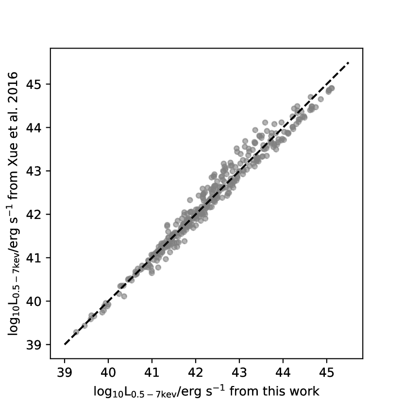
This method does not take into account the intrinsic absorption in obscured sources; however, across the whole sample the X-ray data are not of sufficient quality to allow an in-depth spectral analysis, nor would this significantly affect the luminosities calculated. To demonstrate this, we investigate derived X-ray luminosities for sources in the CDFN field, in which the deep 2 Ms survey data allow a more complete analysis. We compare our PIMMS derived X-ray luminosities in this field with those of Xue et al. (2016), who calculate X-ray luminosities using the hard- and soft-band count ratios to correct for intrinsic absorption (Fig. 1). Our simpler method produces $L_{\mathrm{X}}$ values close to one-to-one with the Xue et al. (2016) values, with an RMS of 0.18 dex. In subsequent analysis, we divide our sample into bins of $\sim 0.8$ dex in log $L_{\mathrm{X}}$, so this level of deviation in our calculated $L_{\mathrm{X}}$ values will have little impact on our results. As such this simple method is sufficiently accurate for this work, and allows for consistency across all survey fields in this study.

Figure 1: CDFN log $L_{\mathrm{X}}$ values derived in this work, compared with values from Xue et al. (2016) which are corrected for intrinsic absorption. The grey dashed line shows 1:1.

Figure 2: Distribution of sources in redshift and X-ray luminosity. The dashed lines show the ranges of redshift and $L_{\mathrm{X}}$ within which the sample is selected. Round points show sources included in the multi-wavelength sample; crosses are sources that are only in the preliminary sample.

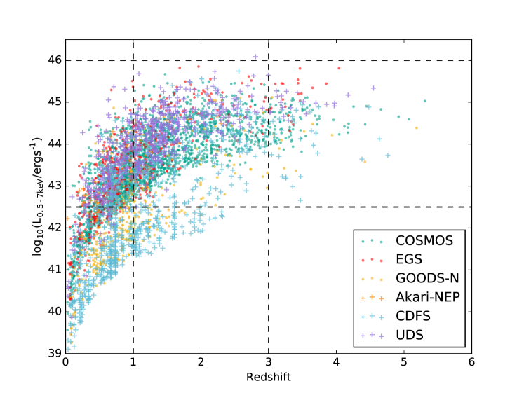
We select sources with a luminosity range of 42.5 < log ($L_{\mathrm{X}}$/erg  s^-1 ) < 46, the lower limit chosen to exclude starburst galaxies. We choose a redshift range $1<z<3$ to probe the epoch of the peak of SFR density and BH accretion rate density in the universe. The distribution of sources in $z$ and $L_{\mathrm{X}}$ space is shown in Fig. 2. The full sample of all six fields contains 1957 X-ray sources within these redshift and X-ray luminosity ranges.

2.3 S2CLS

The SCUBA-2 Cosmology Legacy Survey is a large area ($\sim$5 deg²), deep 850 $\upmu$m survey of several well-studied extragalactic fields. There are several benefits to using S2CLS to investigate star formation at high redshift rather than previous FIR surveys such as Herschel. Tracing star formation at long wavelengths (e.g. 850 $\upmu$m with SCUBA-2, compared to 500 $\upmu$m, the longest Herschel SPIRE wavelength) probes the tail end of the spectrum of cold dust associated with ongoing star formation, and is less likely to suffer from contamination from AGN-heated dust than shorter wavelengths even at high redshifts. At $z=3$, observed 850 $\upmu$m corresponds to rest-frame 212 $\upmu$m, while 500 $\upmu$m corresponds to rest-frame 125 $\upmu$m emission in which part of the spectrum an AGN contribution may be significant (Symeonidis et al., 2016).

SCUBA-2 also affords improved resolution at long wavelength, with a beam FWHM of 14.8 arcsec, compared to the Herschel SPIRE beam FWHM of 36.4 arcsec at 500 $\upmu$m (Griffin et al., 2010).

Additionally, over the redshift range used in this study ($1<z<3$), the negative K-correction (Blain & Longair, 1993) results in 850 $\upmu$m flux that does not diminish with redshift for a given luminosity. Thus a simple comparison of fluxes may be made as a preliminary analysis (see section 3.3).

2.4 LABOCA data

We also use submm data from the LABOCA survey of the ECDFS at 870 $\upmu$m (Weiss et al., 2009), as the CDFS X-ray survey is the deepest available X-ray survey data, with an exposure time of 7 Ms. While the LABOCA data are of lower resolution, with a beam width of 19.2 arcsec, the are the highest quality submm data available for the CDFS, and including this field in our sample allows us to probe the low X-ray luminosity, high $z$ parameter space that would otherwise be excluded. The LABOCA ECDFS catalogue contains 126 submm detected sources at $>3.7\sigma$.

2.5 FIR data

To investigate the FIR spectrum of our sources, we take advantage of the wealth of Herschel and Spitzer data available.

Herschel-SPIRE maps at 500, 350 and 250 $\upmu$m come from the HerMES survey (Oliver et al., 2012). SPIRE maps are in units of Jy/beam, and so fluxes are extracted from the central pixel of stacked images (see section 3.3 for further details on the stacking procedure).

We use combined Herschel-PACS data from the PEP Lutz et al. (2011) and GOODS-Herschel Elbaz et al. (2011) programs, as described in Magnelli et al. (2013). To extract 100 and 160 $\upmu$m fluxes from the PACS maps, we perform aperture photometry following the guidelines in the PEP DR1 readme; for the 100 $\upmu$m and 160 $\upmu$m maps, we use aperture radii of 7.2 and 12 arcsec, respectively.

We also use Spitzer-MIPS (Rieke et al., 2004) maps at 24 and 70 $\upmu$m from the S-COSMOS (Sanders et al., 2007) and FIDEL (Dickinson et al., 2006) surveys. 24 $\upmu$m data for the GOODS-N field are from the GOODS survey (Dickinson et al., 2003). Again we perform aperture photometry on the MIPS maps. By comparing extracted fluxes with those of catalog sources in these maps, we determine the most accurate aperture radii, and use radii of 3.5 and 16 arcsec at 24 and 70 $\upmu$m respectively.

For each of the 8 FIR and submillimetre wavelengths, we verify that there is no significant systematic positional offset ( $\leq 1$ pixel) by performing a median stack at all X-ray source positions and examining the centroids of the resulting images.

3 Results and discussion

3.1 Detection rates of submillimetre sources

We first explore the fraction of sources that are detected in the S2CLS catalogues. The catalogues use a detection threshold of 3.5$\sigma$ (Geach et al., 2017). As the S2CLS survey fields are of slightly different depths, we impose a lower threshold on noise of 1.2 mJy beam^-1, the average 1$\sigma$ depth of S2CLS, across each field to exclude sources that are detected below this noise level in the deepest fields. To match sources from the submillimetre catalogues to the X-ray positions, we use a matching radius of 4$\sigma_{\mathrm{pos}}$, where $\sigma_{\mathrm{pos}}$ is the positional uncertainty given by the equation:

$$\sigma_{\mathrm{pos}}=\frac{0.6\times\mathrm{FWHM}}{\mathrm{SNR}}$$ (3)

(Ivison et al., 2007).

This results in a mean matching radius of $\sim 7$ arcsec. The Chandra positions are accurate to $\approx 0.5$ arcsec, so we neglect any X-ray positional uncertainty as it is an order of magnitude smaller than the submillimetre positional accuracy. In the case that multiple sources are within the matching radius, we take the closest match. We test the spurious detection rate by matching the S2CLS catalogue positions with a randomly generated set of coordinates of the same size as the source list, repeating this procedure 1,000 times. This results in a spurious matching fraction of 1 per cent. We also include the ECDFS field using the LABOCA catalogues (see section 2.4).

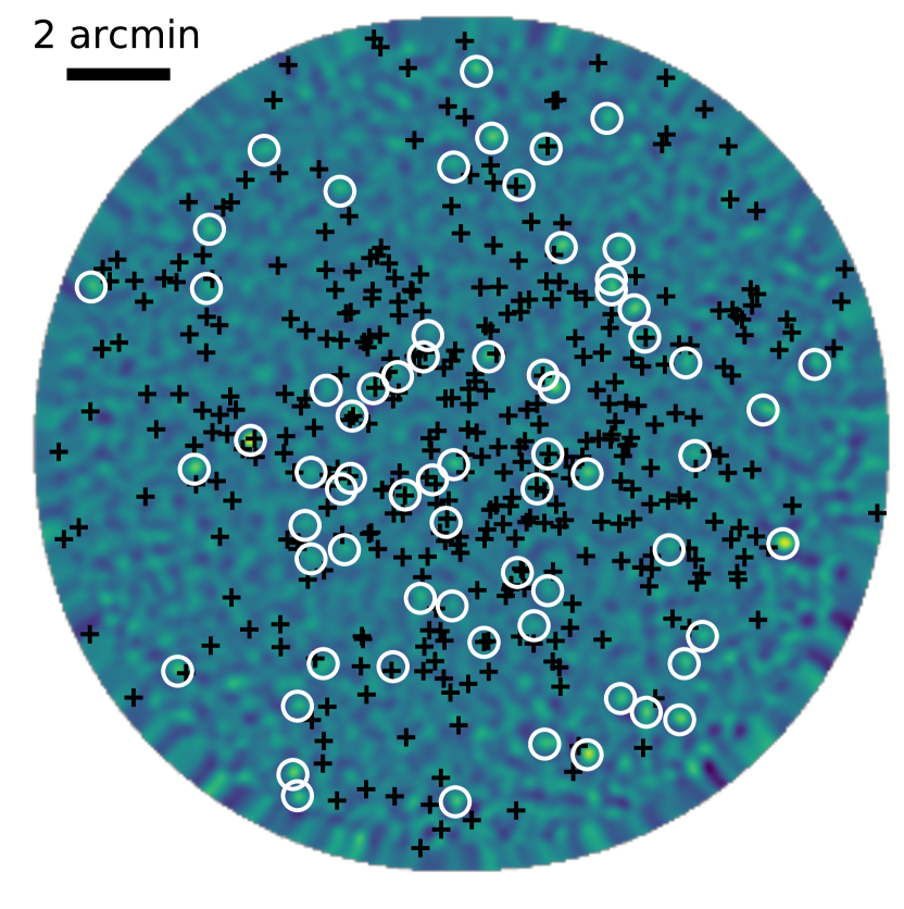
Using this matching criterion, we find that 39 sources are detected at 850 $\upmu$m, 2 per cent of the whole sample. Fig. 3 shows an example S2CLS field (GOODS-N), with submillimetre detections marked with white circles, and X-ray detections marked with black crosses.

Figure 3: The S2CLS map of the GOODS-N field. Submillimetre detections from the S2CLS catalogue (>3.5 $\sigma$) are marked with white circles, and X-ray detections are marked with black crosses. Where there are two X-ray sources within the matching radius of an S2CLS source, the nearest match is assumed to be the correct counterpart. The majority of X-ray sources are not detected at 850 $\upmu$m at the 3.5 $\sigma$ level.

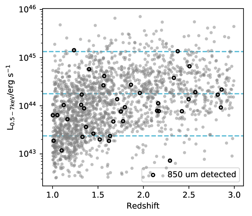
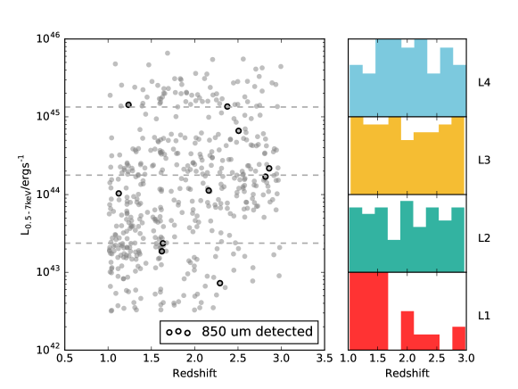
We split the sample into four $L_{\mathrm{X}}$ bins, spaced equally in the log $L_{\mathrm{X}}$ range of the sample, and investigate whether the detection fraction varies with X-ray luminosity. Fig. 4 shows the positions of the submillimetre detected sources in redshift and $L_{\mathrm{X}}$ space. We construct a contingency table of the numbers of detections and non-detections in each $L_{\mathrm{X}}$ bin, shown in Table 2. In contrast to Page et al. (2012), we find similar detection fractions across all X-ray luminosities; the highest luminosity bin has the highest detection fraction (2.53 per cent) but also contains the smallest number of sources. We perform a $\chi^{2}$ test of independence on the contingency table, to investigate whether the difference in detection fractions is significant betweeen the luminosity bins. Assuming that there is no trend with $L_{\mathrm{X}}$, this results in a $p$-value of 0.43, thus we cannot reject the null hypothesis that the detection fraction is independent of $L_{\mathrm{X}}$. Moreover, a $\chi^{2}$ test for trend across the $L_{\mathrm{X}}$ bins results in a $p$-value of 0.83, thus we cannot reject the null hypothesis that there is no trend in the number of detections with $L_{\mathrm{X}}$.

While the detection fraction at 850 $\upmu$m is very low (2 per cent), it is double the spurious detection rate, implying that we do see some real submillimetre sources associated with X-ray positions. However, it is worth noting that this kind of source-by-source analysis is severely limited by the quality of the data, and alone cannot be used to draw a conclusion that is statistically robust. This motivates the use of a stacking analysis (see section 3.2), which, although coarser, is a useful method given the challenge that these data pose for individual source statistics.

Figure 4: Sources detected (black open circles) or undetected (grey circles) at 850 $\upmu$m across all fields, in z/$L_{\mathrm{X}}$ space. The boundaries marking each of the four $L_{\mathrm{X}}$ bins are marked by dashed lines.

Table 2: Number of X-ray sources, and those with submillimetre detections, in each $L_{\mathrm{X}}$ bin. Column 1 shows the range in $L_{\mathrm{X}}$ of each bin, column 2 shows the number of sources, column 3 shows the number of 850 $\upmu$m detections, column 4 shows the detection fraction as a percentage, and column 5 shows the median redshift in each bin.

log $L_{\mathrm{X}}$(erg  s-1)	no. sources	850 $\upmu$m?	%	$z_{\mathrm{m}}$
42.5 – 43.4	321	7	2.18	1.19
43.4 – 44.3	865	21	2.43	1.45
44.3 – 45.1	692	9	1.30	1.80
45.1 – 46	79	2	2.53	2.05

3.1.1 Redshift dependence

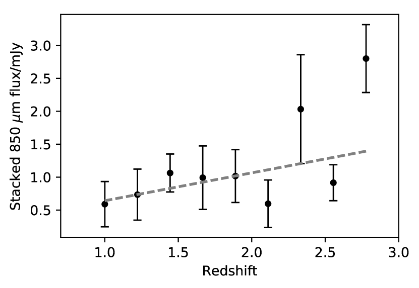
In this analysis, we have not taken into account any selection effects due to the redshift distribution of sources; the highest luminosity bin has a higher median redshift ($z=2.05$) than the lowest bin ($z=1.19$), see Table 2. Any relationship therefore between redshift and 850 $\upmu$m flux is neglected. However, a correlation is to be expected given the increasing number density of submillimetre sources from $1<z<3$ (e.g. Chapman et al., 2005), and the redshift evolution of SFR (e.g. Blain et al., 1999). In Fig. 5 we show the stacked submillimetre flux binned by redshift, and indeed there is a positive correlation between submillimetre flux and redshift. The Pearson coefficient for these data is 0.67; a weighted least squares fit gives a slope of 0.42.

Figure 5: Stacked 850 $\upmu$m flux with redshift. The dashed line shows a weighted least squares fit to the data points, which gives a slope of 0.42; errorbars show 1-$\sigma$ uncertainties on the stacked fluxes.

To account for this, we perform the same analysis on a matched sample that is evenly distributed in redshift space across each of the $L_{\mathrm{X}}$ bins. The distribution of redshifts in each bin of the matched sample is shown in the right panel of Fig. 6. With the exception of the lowest luminosity bin, which simply does not have enough high redshift sources to create a significant evenly distributed sample, the distributions are matched in their redshift distributions. A two sample Kolmogarov-Smirnov test, testing each bin against the 3rd luminosity bin, as an example, shows that we cannot reject the null hypothesis that each sample is drawn from the same distribution. The left panel of Fig. 6 shows the results of matching detections in this evenly distributed sample. Again, we find a higher detection fraction ($\sim$ 2.8 per cent) in the highest luminosity bin; again this bin has the smallest sample size. As in section 3.1,we perform the same $\chi^{2}$ test for independence on the detection fractions across the four bins. Assuming no trend with $L_{\mathrm{X}}$, we obtain a $p$-value of 0.89. Testing for a trend with $L_{\mathrm{X}}$, we obtain a $p$-value of 0.99. Neither allow use to reject the null hypothesis that the detection fraction is independent of $L_{\mathrm{X}}$. Accounting for the redshift distribution of the sources, we find no significant difference in detection rates across the $L_{\mathrm{X}}$ bins (see Table 3).

Figure 6: Left: Sources detected or undetected in submm in z/$L_{\mathrm{X}}$ space for the redshift matched sample. The boundaries marking each of the four $L_{\mathrm{X}}$ bins are marked by grey dashed lines; bin widths are defined by splitting the sample range evenly in log space. Right: Distributions in redshift in each of the 4 $L_{\mathrm{X}}$ bins.

Table 3: Number of X-ray sources, and those with submillimetre detections, in each $L_{\mathrm{X}}$ bin, for the redshift matched sample. Column labelling follows that of Table 2.

log $L_{\mathrm{X}},z$(erg  s-1)	no. sources	850 $\upmu$m?	%	$z_{\mathrm{m}}$
42.5 – 43.4	116	3	2.59	1.52
43.4 – 44.3	169	3	1.78	2.00
44.3 – 45.1	131	7	2.59	1.99
45.1 – 46	71	5	2.82	2.05

3.2 850 $\upmu$m stacked fluxes

As the majority of sources are undetected at submm wavelengths, we divide the sample into bins of X-ray luminosity and stack fluxes in each bin to measure an average flux density.

We begin by investigating the 850 $\upmu$m fluxes. Sources are divided into four bins of X-ray luminosity. For comparison with the latter part of the study, we use the same $L_{\mathrm{X}}$ limits to define bins as in section 3.3, resulting in similar numbers of sources in each bin (see Table 4). We stack at every X-ray position, whether or not the source is detected at 850 $\upmu$m. 100 $\times$ 100 arcsec images are cut around each X-ray position. We begin by calculating both a linear mean and median stack, by calculating the mean/median pixel values. An ‘average’ image is therefore created, for each bin in $L_{\mathrm{X}}$. Examples of median stacked images in each bin are shown in Fig. 7.

Figure 7: Median stacked images for each $L_{\mathrm{X}}$ bin (see Table 4). Each image is 100 $\times$ 100 arcsec.

Table 4: Stacked 850 $\upmu$m flux in each of four $L_{\mathrm{X}}$ bins. Column 1 shows the name of the bin, column 2 the range of X-ray luminosities, column 3 shows the number of sources in each bin and column 4 shows the 850 $\upmu$m median stacked flux in mJy.

$L_{\mathrm{X}}$ bin	$L_{\mathrm{X}}$ range ($10^{43}$ erg  s-1 )	no. sources	median flux (mJy)	mean flux (mJy)
L1	0.351 – 3.48	359	$0.30_{-0.12}^{+0.22}$	$0.45_{-0.04}^{+0.11}$
L2	3.48 – 9.55	389	$0.53_{-0.30}^{+0.24}$	$0.63_{-0.04}^{+0.11}$
L3	9.55 – 26.6	414	$0.50_{-0.19}^{+0.23}$	$0.67_{-0.04}^{+0.11}$
L4	26.6 – 710.	474	$0.48_{-0.15}^{+0.22}$	$0.61_{-0.03}^{+0.09}$

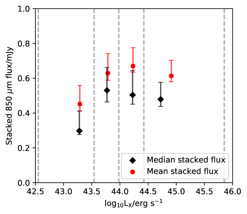
Fig. 8 shows the mean and median stacked fluxes read from the central pixel of each of these images. Uncertainties on these fluxes are calculated via a bootstrap analysis. For each bin, we create a new stack by drawing the same number of images as in the bin randomly and with replacement from the original stack. We then calculate the mean and median stacked fluxes in these new stacks. Repeating this 10,000 times, a distribution of the means/medians is produced, from which we take the 36th and 84th percentiles as the 68 per cent confidence interval, taking this to be equivalent to the 1$\sigma$ uncertainty.

The mean stacked fluxes are strongly biased to higher stacked fluxes by the few very bright submillimetre sources in each stack (e.g. Barger et al., 2015). The median stacks are therefore a more accurate estimator of the average properties of sources binned by $L_{\mathrm{X}}$, robust to bright outliers, and thus we choose to use the median stacks throughout the rest of this work. However, both the mean and median stacked fluxes show the same trend across the $L_{\mathrm{X}}$ bins, and so this choice does not affect the conclusion that we draw from our results. We do not observe a decrease in flux with increasing $L_{\mathrm{X}}$. Instead, the stacked fluxes are consistent with a flat trend within the 68 per cent confidence intervals shown in the highest three bins. Assuming that $L_{\mathrm{X}}$ accurately traces AGN activity, and that 850 $\upmu$m flux is a good tracer of star formation, this result may be interpreted as no evidence that AGN activity suppresses star formation in the galaxies in our sample.

Figure 8: Mean (red circles) and median (black diamonds) stacked 850 $\upmu$m flux with $L_{\mathrm{X}}$. Points are plotted at the mean/median $L_{\mathrm{X}}$ of each bin respectively. Grey dashed lines show the $L_{\mathrm{X}}$ limits of each bin. Error bars show the 1$\sigma$ uncertainties calculated with a bootstrapping analysis.

However, this stacked 850 $\upmu$m flux approach is a simplistic one, and neglects some potentially important factors, namely:

1) We assume that 850 $\upmu$m flux traces star formation alone, and do not account for any contribution to the flux from the AGN torus. While this may be a valid assumption at low $z$, at the high $z$ end of our sample ($z=3$) observed 850 $\upmu$m emission corresponds to 212 $\upmu$m rest-frame emission, which may be affected by a contribution to the flux from the AGN torus (e.g. Symeonidis et al., 2016).

2) The mean redshift of sources in each of the bins changes, with the highest $L_{\mathrm{X}}$ bin containing the most high redshift sources. As such, the part of the SED being sampled at 850 $\upmu$m changes, and this is not taken into account in such a stacking analysis.

To determine a more accurate measure of star-formation rate, we require a method which separates the contributions to the FIR and submm spectrum from the cold dust associated with ongoing star formation, and that from the AGN torus.

3.3 Multi-wavelength stacked fluxes

In order to investigate the FIR/submm spectra of sources in the multi-wavelength sample, we median stack at each of the 8 wavelengths to create average sources to which we can fit SEDs (section 3.4). The sample is first divided into four redshift bins, so that the stacked fluxes can be used for SED fitting without the K-correction becoming significant within each bin; the maximum width of redshift bin is from $2.05<z<3$, which for observed 850 $\upmu$m fluxes corresponds to a range in rest-frame wavelengths of 65 $\upmu$m. These redshift bins are then further subdivided by $L_{\mathrm{X}}$ into four evenly populated bins. This results in 16 bins, each containing $\sim$90 sources (see Table 5).

Table 5: Median properties of each of the 16 bins in redshift and X-ray luminosity. Column 1 shows the redshift range of each bin, column 2 shows the number of sources, column 3 the median redshift, column 4 the median X-ray luminosity in erg  s^-1, and column 5 the calculated SFR in solar masses per year, as described in section 3.5.

z-range	No.	$z_{m}$	$L_{\mathrm{X}}$	SFR
	sources		($10^{43}$ erg  s-1 )	($M_{\odot}$ yr-1)
1 – 1.24	93	1.10	$1.12$	$85_{-5}^{+8}$
	92	1.10	$2.55$	$77_{-12}^{+5}$
	92	1.14	$5.95$	$79_{-5}^{+9}$
	93	1.09	$20.7$	$100_{-14}^{+7}$
1.24 – 1.53	89	1.32	$1.87$	$144_{-25}^{+18}$
	88	1.38	$3.84$	$122_{-22}^{+24}$
	88	1.33	$10.5$	$167_{-28}^{+11}$
	89	1.40	$31.7$	$137_{-12}^{+31}$
1.53 – 2.05	87	1.76	$3.70$	$155_{-23}^{+18}$
	86	1.76	$7.37$	$299_{-43}^{+18}$
	86	1.80	$19.3$	$351_{-64}^{+29}$
	87	1.88	$50.4$	$366_{-37}^{+49}$
2.05 – 3	87	2.47	$7.46$	$592_{-50}^{+95}$
	86	2.53	$15.6$	$600_{-62}^{+141}$
	86	2.39	$30.0$	$453_{-157}^{+71}$
	87	2.45	$110$	$588_{-54}^{+114}$

Following the method outlined in section 3.2, we create median stacked images for each wavelength in each bin, then measure fluxes from these images. For the S2CLS and SPIRE images, the flux is measured at the central pixel of the stacked image. For the MIPS and PACS images, we perform aperture photometry on the stacked images, as described in section 2.5.

At SPIRE wavelengths, there will be a significant contribution to the flux from confusion noise, which may bias our results. We perform a bootstrapping method to estimate the confusion noise in each bin at each wavelength to characterise the noise and to account for this bias. To do so, we bootstrap over stacks at random positions in the survey images. In each bin, we draw an equal number of random positions as the number of sources in the bin, and repeat this random stack 10,000 times. We measure the stacked flux from these random stacks, and use the resulting distribution to characterise the noise. We find that the random stacks are not centered around zero, but rather are offset by some positive flux. This is likely due to blending of faint sources, and as such some positive flux density accumulates in the stacked image. This procedure is performed for each bin at each wavelength. We measure the offsets for each, and subtract them from the measured stacked fluxes, following the procedure of Stanley et al. (2017).

A similar bootstrap procedure is performed to estimate the 1$\sigma$ error on the stacked median fluxes. Again, as each bin contains a different number of sources, we perform this procedure on each bin in each wavelength separately. An equal number of sources as the number of sources in each bin are drawn randomly with replacement from the sample, then the median stacked image is created and the flux measured. We do this 10,000 times to create a distribution of median fluxes, from which we take the 68 per cent confidence interval as a 1$\sigma$ error estimate. The resulting distributions are smooth and gaussian-like for those wavelengths for which we perform aperture photometry (160, 100, 70 and 24 $\upmu$m), but for the wavelengths in which we simply measure the central pixel flux, the possible values for the medians are discrete rather than continuous and as a result the distribution is not smooth. To account for this, we perform a smoothed bootstrap on these four wavelength samples (850, 500, 350 and 250 $\upmu$m), in which we add a small amount of random noise ($\sigma=0.1$) to each measured median stacked flux. This smoothed bootstrap distribution is then smooth and gaussian-like, and representative of the spread of the sample. From this we measure the 68 per cent confidence interval as the 1$\sigma$ error.

Figure 9: Example stacked images in each wavelength. The black bar on each image indicates 25 arcsec scale.

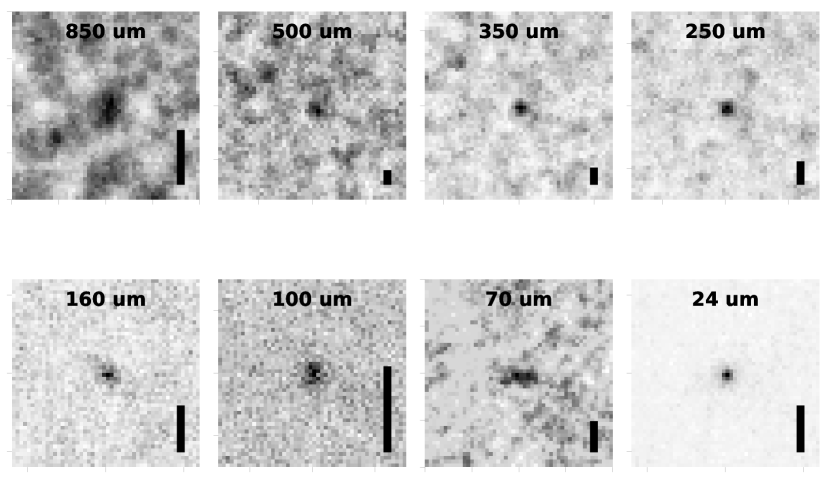
This process results in measured median stacked fluxes for each of the 8 wavelengths, binned by $L_{\mathrm{X}}$ and redshift, creating 16 ‘average’ sources spanning the ranges of $z$ and $L_{\mathrm{X}}$ of interest.

3.4 SED fitting

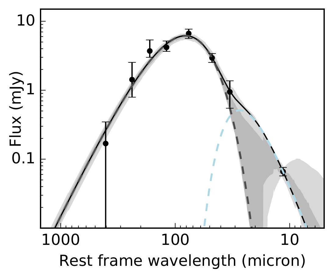
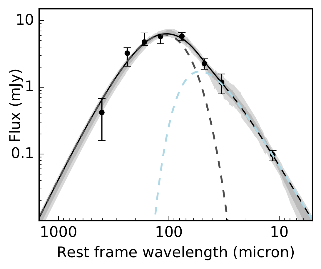
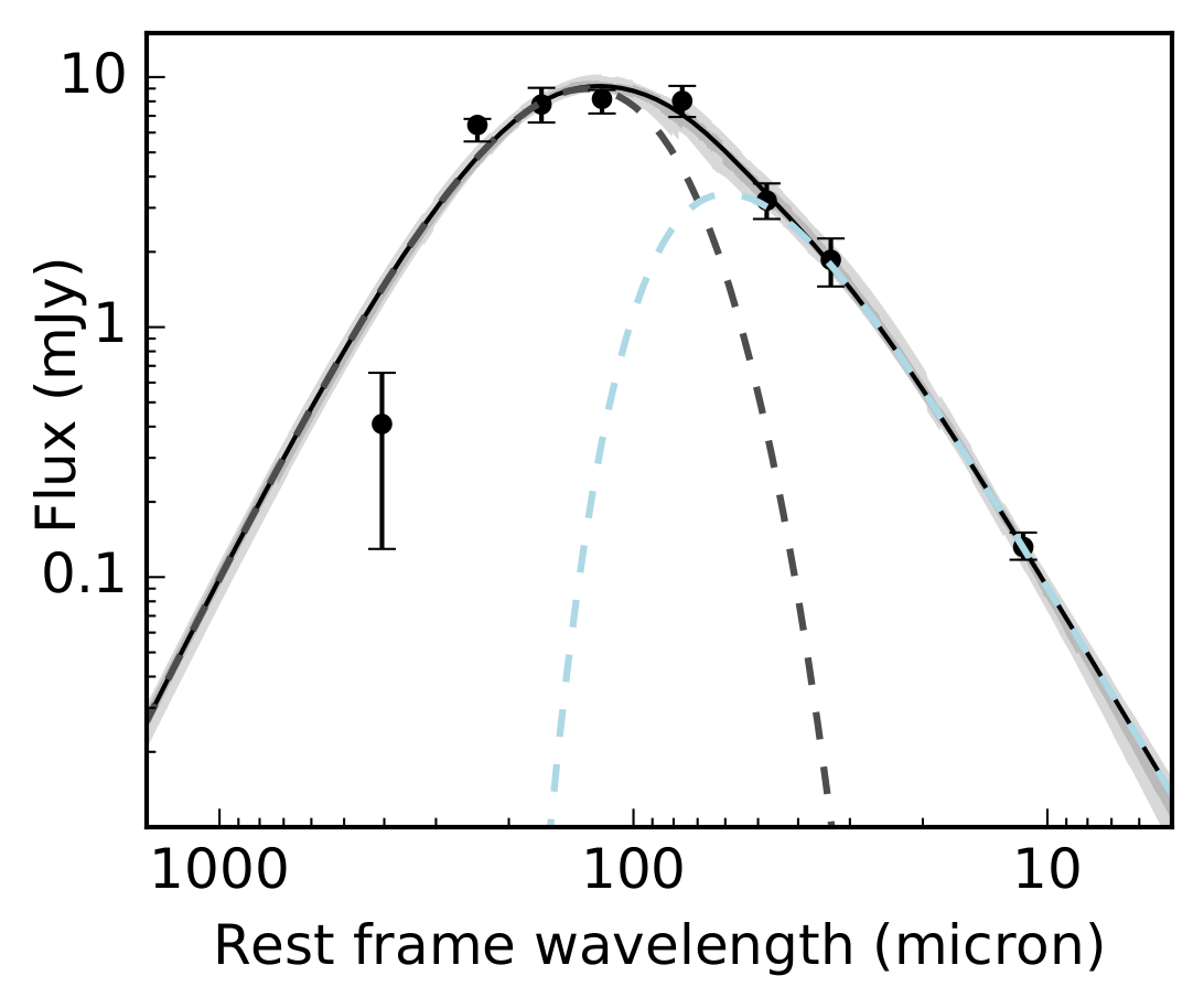
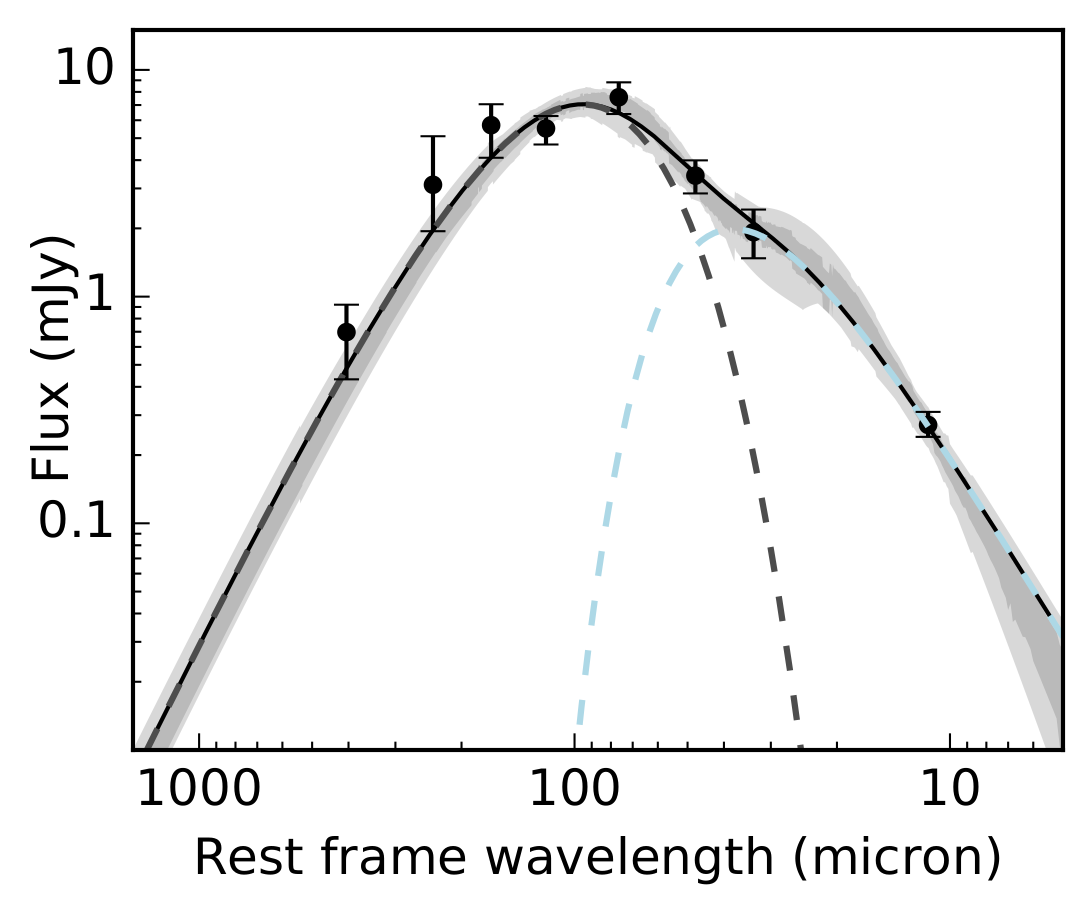
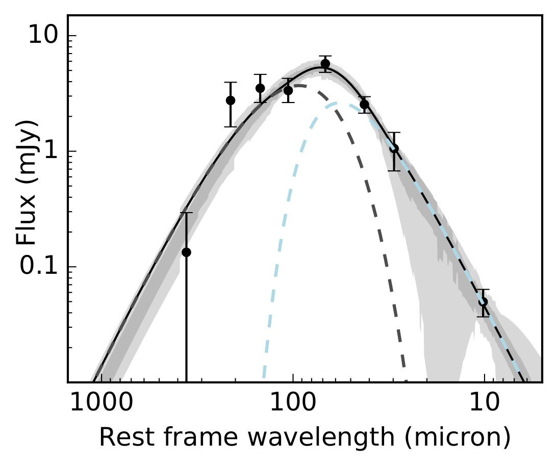
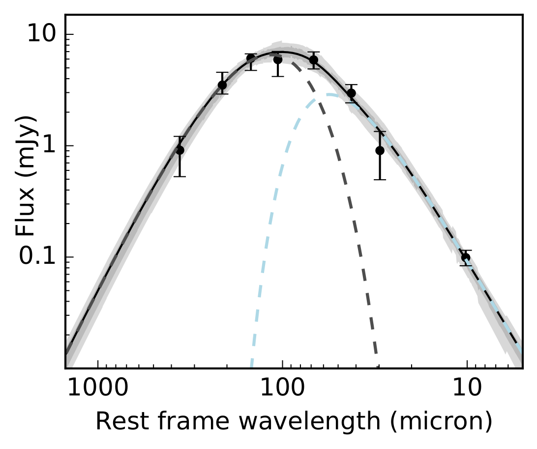
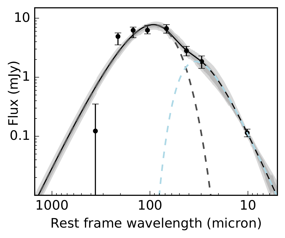
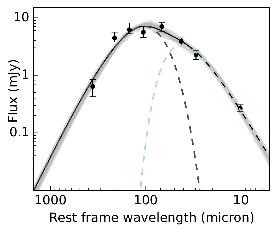
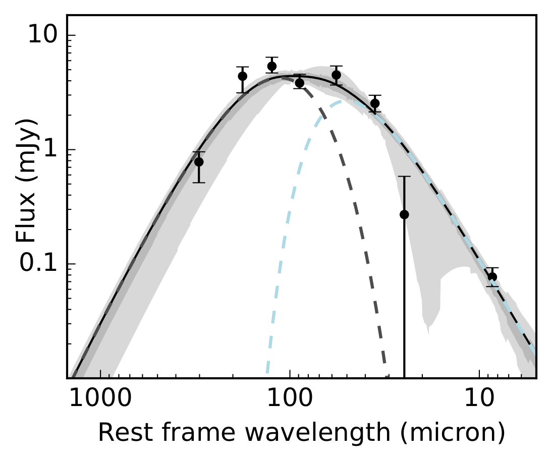
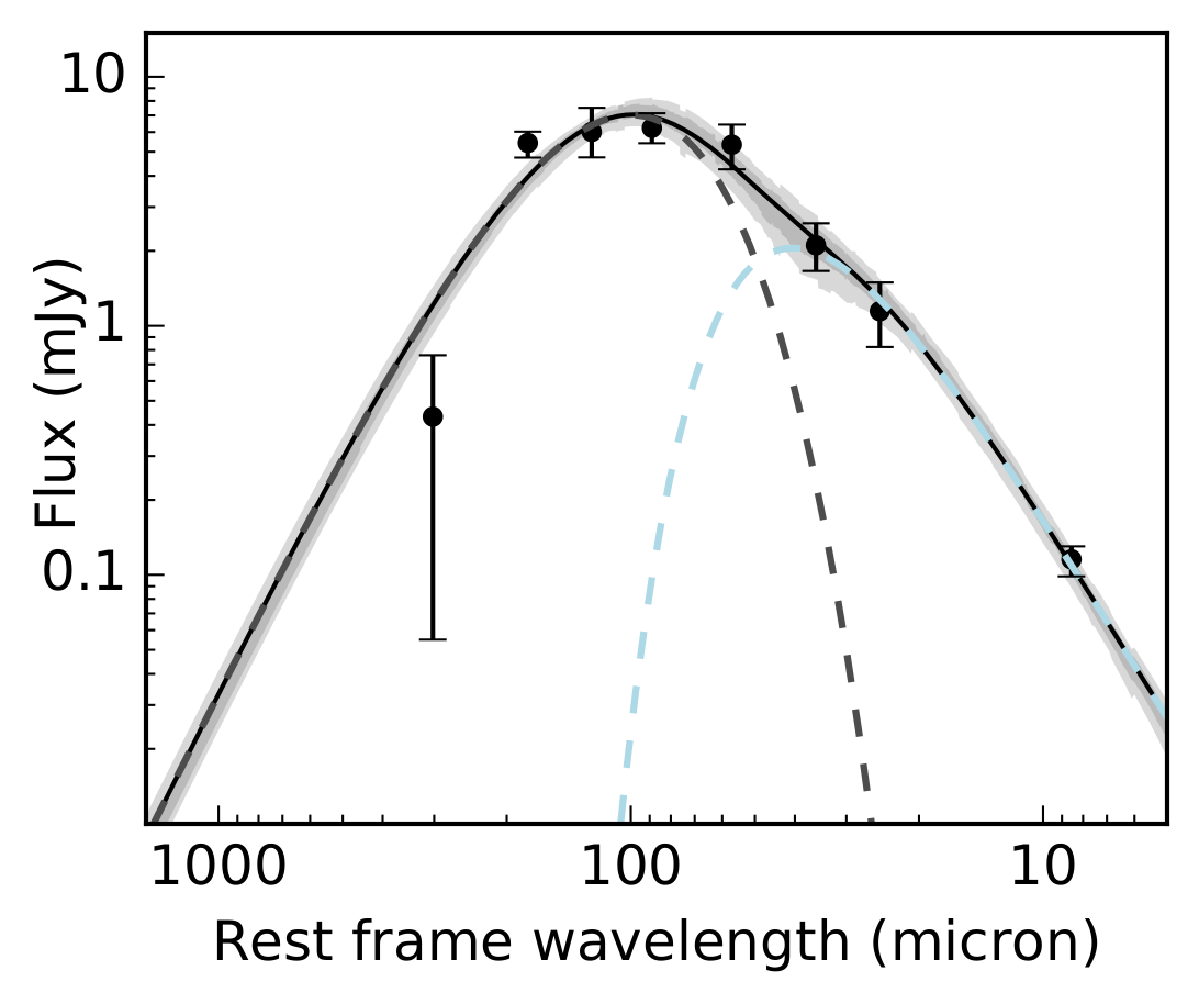
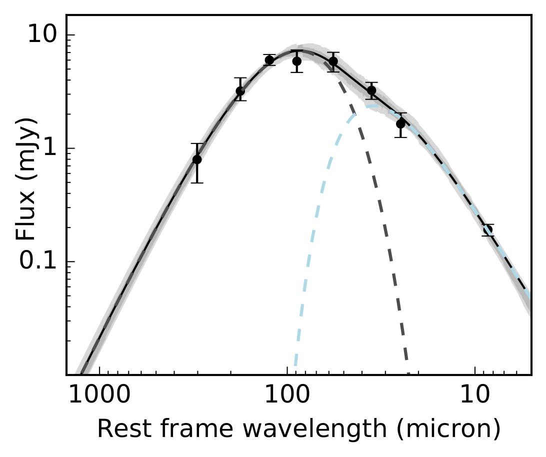
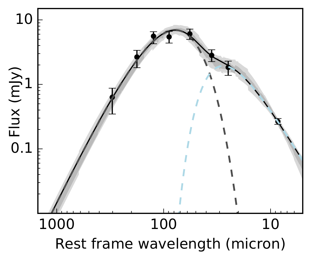
Using the resulting fluxes, we fit an SED to each of the 16 ‘average’ sources. We model the FIR SED as two components: a cold dust greybody contribution, and a warm dust power law contribution, described by the following equation:

$$S(\lambda)=N_{\mathrm{gb}}\frac{(\frac{c}{\lambda})^{\beta+3}}{e^{\frac{hc}{\lambda kT}}-1}+N_{\mathrm{pl}}\lambda^{\alpha}e^{-\frac{\lambda}{\lambda_{\mathrm{c}}}^{2}}$$ (4)

simplified assuming the optically thin case, where $S(\lambda)$ is the flux in Jy, $N_{\mathrm{gb}}$ and $N_{\mathrm{pl}}$ are a normalization coefficients of the greybody and power law components respectively, $T$ is the temperature of the greybody, $\beta$ is the emissivity index of the dust grains, $\alpha$ is the slope of the power law, and $\lambda_{\mathrm{c}}$ is the cut-off wavelength of the power law (Casey, 2012). We fix $\beta$ to be 1.5, a value widely assumed in the literature (e.g. da Cunha et al., 2008; Casey, 2012). Following arguments in Smith et al. (2013), allowing $\beta$ to be a free parameter would have little impact on our derived FIR luminosities. This leaves five free parameters for the fit: $N_{\mathrm{gb}}$, $N_{\mathrm{pl}}$, $T$, $\alpha$ and $\lambda_{\mathrm{c}}$.

Fitting an analytical form of the SED, rather than using a library of templates, is a sensible choice here as (a) the data are not sufficiently high-resolution to warrant fitting to the level of detail of empirical templates, and (b) this removes biases introduced by choice of templates, which include restricting the AGN contribution to the spectrum (see below), and allows us to test a more flexible model. Our results are in good agreement with studies such as Stanley et al. (2015) and Suh et al. (2017) that use a template fitting approach (see section 3.5 and Fig. 11), suggesting that template fitting is not necessary to decompose the FIR spectrum.

We choose to model a single warm dust component with a power law with exponential cutoff, and a single cold dust component with the greybody function, and do not include any additional component representative of kpc-scale dust heating by the AGN (Symeonidis et al., 2016). However, in contrast to previous analytical approaches (e.g. Barger et al., 2015), we do not fix the cut-off wavelength of the power law component $\lambda_{\mathrm{c}}$, allowing this as a free parameter. Fixing $\lambda_{\mathrm{c}}$ to a given wavelength risks underestimating the AGN contribution to the FIR SED, so by keeping it as a free parameter we allow for the case in which the AGN contributes the majority of the FIR emission. We do however restrict the peak of the power law component to fall at shorter wavelengths than the peak of the greybody, which avoids non-physical fits while allowing the possibility that either component dominates the spectrum. Nevertheless, our resulting best-fitting average SEDs are consistent with a single warm component plus a significant greybody contribution from cold dust associated with star formation, with all of our fits favouring a significant cold component in the submillimetre spectrum.

We assume that the cold dust component may be attributed to heating from star-formation processes only, and that the warm dust component is likely have a significant contribution from the AGN. Under this assumption, we estimate SFRs using the cold dust component only (see section 3.5. This method neglects any warm dust contribution from star formation, and as such we may underestimate the SFRs. As a test, we calculate SFRs using both the warm and cold components, for the case that all FIR emission is due to star formation, which results in SFRs higher than our reported values by a factor of 2 at most. Excluding the warm component from the SFR calculation reduces the likelihood of overestimating SFRs in the case of a significant AGN contribution.

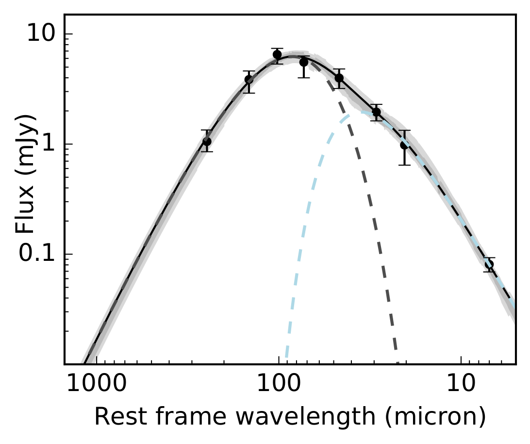
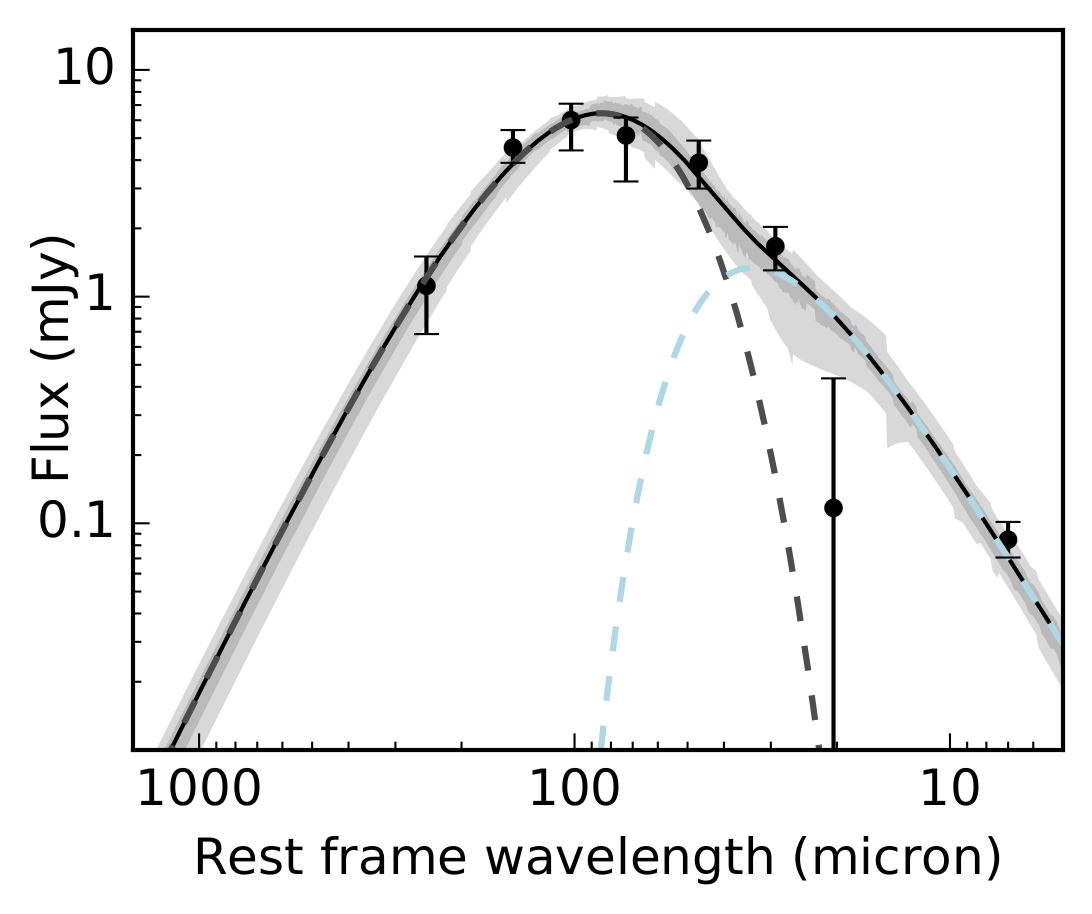
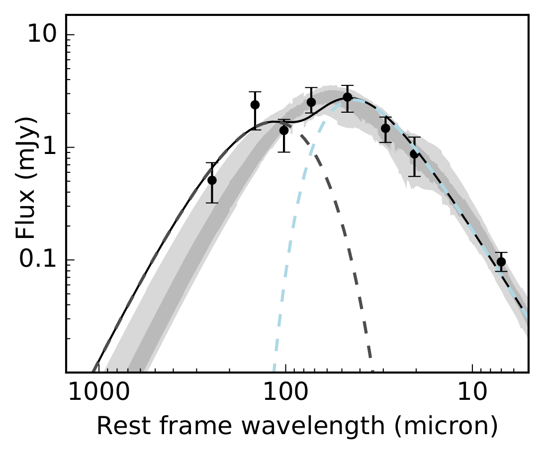
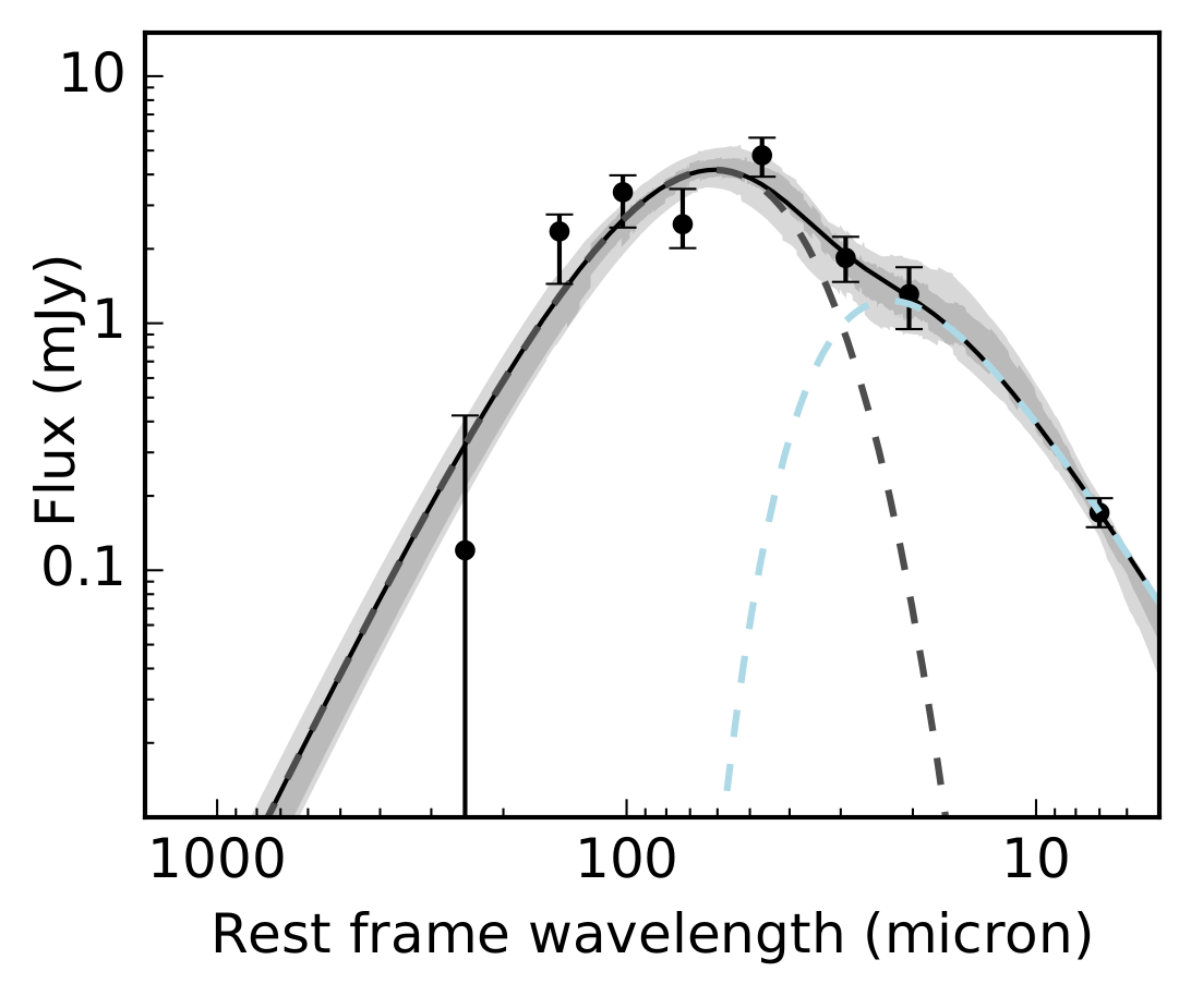
We follow an MCMC fitting procedure using the emcee Python code (Foreman-Mackey et al., 2013). This allows a fully Bayesian approach, giving a robust characterisation of the uncertainties of the fit. Walkers are distributed with a truncated normal distribution across the prior parameter space, with priors set to exclude non-physical solutions. We state the modes of the posterior probability distributions of each parameter in Table 6. Uncertainties on these values are taken as the Highest Posterior Density (HPD) 68 per cent credible interval. The uncertainties on the fit are determined by taking the HPD 68 per cent credible interval at each wavelength. Fig. 10 shows fitted SEDs for each of the 16 ‘average’ sources, with the median stacked flux data points in black. The light blue and grey dashed lines show the warm and cold dust contributions to the fit respectively, with the solid black line showing the maximum likelihood solution. The grey shaded areas show the 68 per cent and 95 per cent credible intervals from the HPD at each wavelength.

Table 6: Table of fit parameters, showing the modes of the posterior probability distributions for each parameter, for each of the 16 ‘average’ sources fitted, as well as the median redshift $z_{m}$ and X-ray luminosity $L_{\mathrm{X}}$ for each bin as in Table 5. $\mathrm{log}\>N_{\mathrm{gb}}$ is the normalization of the greybody component, $T$ the greybody temperature, $\mathrm{log}\>N_{\mathrm{pl}}$ the normalization of the power law component, and $\alpha$ and $\lambda_{\mathrm{c}}$ are the slope and cutoff wavelength of the power law component respectively. Errors stated are the 68 per cent credible intervals calculated from the HPDs.

$z_{m}$	$L_{\mathrm{X}}$ ($10^{43}$ erg  s-1 )	$\mathrm{log}N_{\mathrm{gb}}$	$T$(K)	$\mathrm{log}N_{\mathrm{pl}}$	$\alpha$	$\lambda_{\mathrm{c}}$ ($\upmu$m)
1.10	$1.12$	-130.89 ${}_{-0.20}^{+0.17}$	40.24 ${}_{-1.60}^{+1.41}$	24.37 ${}_{-2.97}^{+13.58}$	2.97 ${}_{-0.25}^{+1.21}$	-10.92 ${}_{-0.83}^{+0.30}$
1.10	$2.55$	-129.77 ${}_{-0.24}^{+0.28}$	31.60 ${}_{-2.07}^{+2.07}$	22.78 ${}_{-0.79}^{+7.65}$	2.81 ${}_{-0.08}^{+0.66}$	-10.33 ${}_{-0.28}^{+0.28}$
1.14	$5.95$	-128.39 ${}_{-0.16}^{+0.13}$	25.13 ${}_{-0.99}^{+1.02}$	22.91 ${}_{-0.52}^{+2.03}$	2.80 ${}_{-0.05}^{+0.18}$	-9.94 ${}_{-0.12}^{+.09}$
1.09	$20.7$	-130.27 ${}_{-0.24}^{+0.27}$	37.00 ${}_{-2.78}^{+1.61}$	22.95 ${}_{-0.50}^{+10.16}$	2.74 ${}_{-0.05}^{+0.88}$	-10.57 ${}_{-0.30}^{+0.16}$
1.32	$1.87$	-131.50 ${}_{-0.30}^{+0.36}$	44.86 ${}_{-4.17}^{+2.86}$	25.75 ${}_{-3.31}^{+10.82}$	3.09 ${}_{-0.30}^{+0.94}$	-10.86 ${}_{-0.25}^{+0.98}$
1.38	$3.84$	-129.39 ${}_{-0.35}^{+0.26}$	29.97 ${}_{-2.95}^{+2.22}$	23.04 ${}_{-0.50}^{+2.54}$	2.81 ${}_{-0.05}^{+0.22}$	-10.06 ${}_{-0.19}^{+0.14}$
1.33	$10.5$	-130.14 ${}_{-0.17}^{+0.31}$	35.29 ${}_{-2.51}^{+1.77}$	23.99 ${}_{-1.05}^{+11.14}$	2.85 ${}_{-0.07}^{+0.98}$	-10.59 ${}_{-0.21}^{+0.30}$
1.40	$31.7$	-129.80 ${}_{-0.25}^{+0.26}$	32.57 ${}_{-2.28}^{+2.35}$	23.23 ${}_{-0.38}^{+1.96}$	2.74 ${}_{-0.04}^{+0.17}$	-10.33 ${}_{-0.11}^{+0.12}$
1.76	$3.70$	-129.82 ${}_{-0.29}^{+0.25}$	29.21 ${}_{-1.98}^{+1.92}$	23.40 ${}_{-0.84}^{+2.24}$	2.83 ${}_{-0.08}^{+0.19}$	-10.11 ${}_{-0.10}^{+0.09}$
1.76	$7.37$	-129.83 ${}_{-0.25}^{+0.18}$	32.78 ${}_{-1.58}^{+1.97}$	22.94 ${}_{-0.45}^{+2.28}$	2.75 ${}_{-0.05}^{+0.19}$	-10.36 ${}_{-0.14}^{+0.13}$
1.80	$19.3$	-130.46 ${}_{-0.24}^{+0.22}$	38.25 ${}_{-2.73}^{+2.06}$	23.46 ${}_{-0.41}^{+2.50}$	2.74 ${}_{-0.04}^{+0.21}$	-10.50 ${}_{-0.11}^{+0.13}$
1.88	$50.4$	-131.03 ${}_{-0.26}^{+0.25}$	43.24 ${}_{-3.21}^{+1.99}$	23.47 ${}_{-0.42}^{+6.29}$	2.71 ${}_{-0.04}^{+0.53}$	-10.73 ${}_{-0.20}^{+0.11}$
2.47	$7.46$	-130.74 ${}_{-0.23}^{+0.17}$	39.14 ${}_{-1.97}^{+2.09}$	23.66 ${}_{-0.60}^{+3.45}$	2.79 ${}_{-0.05}^{+0.29}$	-10.51 ${}_{-0.14}^{+0.14}$
2.53	$15.6$	-130.71 ${}_{-0.27}^{+0.35}$	38.25 ${}_{-2.79}^{+3.37}$	23.08 ${}_{-0.69}^{+1.69}$	2.74 ${}_{-0.06}^{+0.15}$	-10.53 ${}_{-0.22}^{+0.15}$
2.39	$30.0$	-133.23 ${}_{-0.47}^{+0.64}$	57.03 ${}_{-9.04}^{+7.03}$	23.69 ${}_{-1.07}^{+8.68}$	2.77 ${}_{-0.09}^{+0.70}$	-10.91 ${}_{-0.44}^{+0.29}$
2.45	$110$	-132.86 ${}_{-0.24}^{+0.37}$	57.72 ${}_{-5.31}^{+3.08}$	23.79 ${}_{-0.46}^{+11.44}$	2.73 ${}_{-0.04}^{+0.95}$	-11.10 ${}_{-0.24}^{+0.21}$

(a)

(b)

(c)

(d)

(e)

(f)

(g)

(h)

(i)

(j)

(k)

(l)

(m)

(n)

(o)

(p)

Figure 10: SED fits for each of the 16 ‘average’ sources. Median stacked fluxes are shown as black points, with associated 1$\sigma$ errors determined by a bootstrapping analysis (see section 3.3). The black solid line shows the maximum likelihood realisation, with the grey dashed line showing the cold dust greybody component and the blue dashed line showing the warm dust power law component. The shaded grey regions show the 68 and 95 per cent credible intervals, calculated from our Bayesian analysis.

3.5 Star-formation rates with AGN luminosity

The FIR luminosity due to SF is calculated by integrating under the greybody curve from 8 to 1000 $\upmu$m. This is done for each realisation of the fit for each of the 16 ‘average’ sources, taking the mode of the resulting distribution and using the 68 per cent credible interval of the HPD as the uncertainty on the FIR luminosity.

SFRs are calculated from this FIR luminosity using the Kennicutt (1998a) relation:

$${\mathrm{SFR}}(M_{\odot}{\mathrm{yr}}^{-1})=4.5\times 10^{-44}L_{\mathrm{FIR}}({\mathrm{erg\>s}}^{-1})$$ (5)

Fig. 11 shows the resulting SFRs calculated for each of the 16 average sources for each redshift and $L_{\mathrm{X}}$ bin.

For comparison, we also plot the results of Stanley et al. (2015). Following Xue et al. (2016), we convert our $L_{0.5-7~{}\rm keV}$ luminosities to equivalent $L_{2-10~{}\rm keV}$ luminosities for the purposes of comparison, assuming a photon index $\Gamma=1.8$, such that:

$$L_{2-10~{}\rm keV}=0.721\times L_{0.5-7~{}\rm keV}$$ (6)

Our results are in good agreement with the study by Stanley et al. (2015), which follows a similar approach with several notable differences. We use analytical models in our SED fitting procedure rather than template fitting. As discussed in section 3.4, this removes the issue of biases regarding the choice of templates used in the fit, however may underestimate SFRs if there is a significant warm dust component from SF. We also make use of newer, deeper X-ray surveys (e.g. Xue et al., 2016; Civano et al., 2016) and as such have a larger sample of sources, so are able to use only spectroscopic redshifts thus more accurately determined X-ray luminosities. Our study extends to slightly higher redshift, spanning an additional $\sim$ 0.5 Gyr in cosmic time, and expanding the parameter space in which this relationship has been investigated. Additionally, using the S2CLS data provides additional information about the Rayleigh-Jeans tail of the dust spectrum, allowing us to closely constrain the fit at long wavelengths. We also follow a median rather than mean stacking approach, which avoids the issue of the few brightest sources in the stack biasing the stacked flux to a higher value (e.g. Barger et al., 2015). Despite these differences in method, our results do agree with those of Stanley et al. (2015), displaying the same flat trend of SFR with $L_{\mathrm{X}}$.

To investigate the systematics of our method, we construct an SED template using Siebenmorgen & Krügel (2007) starburst and Siebenmorgen et al. (2015) AGN torus templates, and extract fluxes at the observed wavelengths. Applying our fitting mechanism to these simulated datapoints, we find that we consistently underestimate the template SFRs by a factor of $\sim 30$ per cent. As described in section 3.4, this is to be expected as we do not account for any contribution to the MIR spectrum from SF. However, as we are largely interested in the trend of SFR with $L_{\mathrm{X}}$ rather than absolute SFRs, this systematic discrepancy does not affect our overall conclusion. We also investigate whether varying $\beta$ has a significant impact on our fitted SFRs; across the range $1<\beta<2$ we find the resulting SFR varies by a factor of $\sim 10$ per cent and similarly does not affect our conclusion.

Figure 11: SFR versus X-ray luminosity, for each of the 16 median ‘average’ sources. Circles show this work, with 1$\sigma$ errors; where not visible, errors are within the size of the points. Crosses are from Stanley et al. (2015). Colours indicate redshift; the Stanley et al. (2015) sample covers a redshift range $0.2<z<2.5$. There is no evidence for a decrease in SFR with increasing AGN power, and within each redshift bin there is no significant positive or negative trend of SFR with $L_{\mathrm{X}}$.

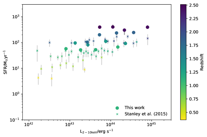
As in section 3.2, we find no decrease in SFR with increasing $L_{\mathrm{X}}$. Across the redshift range of the whole sample, there is a mild positive slope with SFR increasing with $L_{\mathrm{X}}$. In previous work (e.g. Stanley et al., 2015, 2017), this positive slope has been attributed to the evolution of SFR with stellar mass (the ‘main sequence’ of star-forming galaxies). We do not have reliable stellar masses for the galaxies in our sample, but referring to their work, this explains well the trend that is observed. In Stanley et al. (2017), stellar mass is inferred from black hole mass $M_{\bullet}$. Selecting sources by their X-ray flux results in the selection effect that the highest $L_{\mathrm{X}}$ sources in our sample are those objects that have both the highest Eddington ratios, and the highest $M_{\bullet}$, thus higher stellar masses, assuming the stellar mass – $M_{\bullet}$ relation. Galaxies of higher $L_{\mathrm{X}}$ are therefore typically those with higher $M_{\bullet}$ and inferred stellar mass, which corresponds to higher SFR. Additionally, with increasing redshift bins we have both the selection effect that we select a greater number of more luminous sources when probing a larger volume, and the effect of the redshift evolution of the SF main sequence (e.g. Noeske et al., 2007). Thus we can draw the conclusion, following Stanley et al. (2017), that the AGN in our sample reside in normal star-forming galaxies, and the trend of SFR – $L_{\mathrm{X}}$ can be attributed to the star forming main sequence of galaxies. Within each redshift bin, the SFR is consistent with a flat trend with $L_{\mathrm{X}}$, within errors. The only exception is the $1.53<z<2.05$ bin in which there is a slight positive trend.

Notably, we do not see any negative correlation between SFR and $L_{\mathrm{X}}$ that we might interpret as evidence that the most powerful AGN quench star formation in their host galaxies. This work adds to a number of recent studies that have markedly not observed this anticorrelation (e.g. Stanley et al., 2017; Suh et al., 2017; Scholtz et al., 2018).

There are a number of explanations for this lack of signature. It may be due to the time-scales of AGN activity relative to star formation (Hickox et al., 2014; Harrison, 2017): interpreting this relationship as evidence of negative AGN feedback or lack thereof requires the assumption that instantaneous X-ray luminosity is a reliable indicator of AGN activity. However, X-ray luminosity can vary by several orders of magnitude over very short time-scales ($10^{3}-10^{6}$ years) due to the stochastic nature of AGN fueling, relative to much longer time-scales associated with star formation and quenching ($\sim 10^{8}$ years, e.g. Hickox et al., 2014). As such, instantaneous X-ray luminosity does not reliably trace long-term average BHAR, and we do not necessarily expect to see a negative correlation between SFR and $L_{\mathrm{X}}$ as an indication of suppressed star formation.

One way to investigate the observational effects of AGN feedback-driven quenching is by comparing observations to the results of large-scale cosmological simulations. We perform a simple comparison, using the results of the Horizon-AGN simulation (Dubois et al., 2014).

Figure 12: SFR versus X-ray luminosity, for both the observational data (filled circles) and the simulated Horizon-AGN galaxies (dots, with binned values shown with filled diamonds), for each redshift bin. Colours correspond to redshifts in Fig. 11. Both observations and simulations show, within each redshift bin and across this $L_{\mathrm{X}}$ range, a flat trend of SFR with increasing $L_{\mathrm{X}}$.

3.5.1 The Horizon-AGN simulation

The Horizon-AGN simulation is large-scale hydrodynamical cosmological simulation, tracing the stellar mass growth of galaxies from redshift $z\sim 6$. It successfully reproduces observable galaxy properties such as the stellar mass and luminosity functions and cosmic star formation history (Kaviraj et al., 2017), as well as BH demographics such as the cosmic evolution of BH mass density and BH – host galaxy correlations (Volonteri et al., 2016; Martin et al., 2018). Although the model is described in detail in Dubois et al. (2014) and Kaviraj et al. (2017), we briefly outline the treatment of BHs and star formation here as these are relevant to the observable quantities in this study.

Star formation follows a standard Kennicutt (1998b) law with 2 per cent efficiency, when the hydrogen density exceeds $n_{0}=0.1$ H cm^-3. Stellar feedback is implemented via a subgrid model which includes all processes that contribute to thermal and kinetic feedback on ambient gas (see Kaviraj et al., 2017).

BHs with initial mass 10⁵ $M_{\odot}$ are seeded as ‘sink’ particles where local gas density exceeds $\rho>\rho_{0}$ , and stellar velocity dispersion exceeds 100 km s^-1, where $\rho_{0}=1.67\times 10^{-25}$ g cm^-3 and corresponds to 0.1 H cm^-3. BHs grow through both gas accretion, which follows a Bondi-Hoyle-Lyttleton model with accretion capped at the Eddington limit, and through mergers (Dubois et al., 2014; Dubois et al., 2016).

Two modes of BH feedback are implemented, based on the accretion efficiency $\chi=\dot{M}_{\mathrm{BH}}/\dot{M}_{\mathrm{Edd}}$. At low accretion efficiencies ($\chi<0.01$), a ‘radio’ mode feeds energy into the surrounding medium via bipolar outflows, with jet velocities of $10^{4}$ km s^-1. A ‘quasar’ mode takes over at high accretion efficiencies ($\chi<0.01$), modelled as an isotropic thermal energy injection of 1.5 per cent of the accretion energy into the surrounding gas.

3.5.2 Bolometric correction

We calculate BH bolometric luminosities assuming a radiative efficiency of 10 per cent (Shakura & Sunyaev, 1973) and use the recommended bolometric corrections for radio-loud and radio-quiet quasars from Runnoe et al. (2012, Equation 14 and 15) to convert these bolometric luminosities to $L_{2-10~{}\rm keV}$. For BHs with Eddington ratios where $\chi>0.01$ (quasar-mode) we use the radio-loud correction, while for those with Eddington ratios where $\chi<0.01$ (jet-mode) we use the radio quiet correction. Using these corrections, we are able to reproduce the approximate normalization (to within 1 dex, across the full range of $L_{\mathrm{X}}$ considered in this study) and slope of the observed X-ray luminosity function at $z\sim 4$ (e.g. Georgakakis et al., 2015).

3.5.3 Comparison with observational result

Galaxies in the Horizon-AGN simulated sample are split into bins of 0.5 dex in $L_{\mathrm{X}}$ in the four redshift intervals of the observational sample. Fig. 12 shows SFR plotted against $L_{\mathrm{X}}$, as in Fig. 11, for each bin of the simulated dataset (open diamonds) and the observational result (closed circles; colours correspond to redshift bins). The simulated results, incorporating the AGN feedback model described in Section 3.5.1, also show a flat trend of SFR with increasing $L_{\mathrm{X}}$. It should be noted that, while the trends agree, there is around an order of magnitude discrepancy between the normalization of SFR in the simulation compared to the observations. This discrepancy is not unusual in semi-analytical models and hydrodynamical simulations (e.g. Lamastra et al., 2013; Sparre et al., 2015), and one reason for this may be the star formation prescription. While simulations are capable of reproducing averaged properties such as SFR density, the models of star formation that are used may not accurately reproduce instantaneous star formation properties of individual galaxies, specifically the high SFRs associated with galaxies undergoing a starburst phase. Star formation in the simulation assumes a star formation efficiency of 2 per cent, an assumption that may not be valid across all redshifts. Alternatively, a more complex model of star formation may result in higher peak SFRs.

Nevertheless, SFR shows no increasing or decreasing trend with $L_{\mathrm{X}}$. This is in agreement with McAlpine et al. (2017) and Scholtz et al. (2018), who compare the SFR, specific SFR and X-ray luminosity of a sample of AGN with an equivalent simulated sample from the EAGLE suite of hydrodynamical simulations (Crain et al., 2015). They find that their observational results match closely to that of the simulated sample, whether or not the simulation includes AGN feedback. In neither sample do they observe a trend of decreasing SFR with X-ray luminosity that one might expect in the case of AGN quenching star formation, instead also finding a flat relation. The AGN feedback model implemented in the Horizon-AGN simulation is somewhat more complex than that of EAGLE, which incorporates only one mode of AGN feedback; we also determine SFRs using a different method (as outlined in Section 3.5), and our observational dataset is an order of magnitude larger than that of Scholtz et al. (2018) and extends to higher redshifts than those considered in McAlpine et al. (2017). Despite these differences in approach in both simulation and observation, our result agrees with this previous work. This provides another piece of evidence to suggest that, even with AGN feedback as a fundamental mechanism to quench star formation in galaxy growth, we do not expect to see the observational signature of this in the relation betweeen SFR and instantaneous AGN X-ray luminosity.

3.5.4 No enhanced star formation at high $L_{\mathrm{X}}$

There is also no sign of enhanced SFR in the most luminous AGN, as reported in previous work (e.g. Lutz et al., 2010; Rosario et al., 2012). These studies find a strong correlation between SFR and AGN luminosity only in the most luminous AGN (generally, $L_{\mathrm{AGN}}\gtrsim 10^{44}{\mathrm{erg\>s}}^{-1}$). This has been interpreted as evidence of two modes of AGN – galaxy coevolution, in the two different $L_{\mathrm{AGN}}$ regimes: a secular evolution of SF in the low luminosity regime, and a tight AGN – SFR coevolution in the high luminosity regime. However, studies that find this positive SFR – $L_{\mathrm{AGN}}$ correlation in high luminosity AGN have only examined low redshift ($z<1$) samples; here, we do not find any evidence of this trend at $z>1$. In the context of this two-mode model, it is this secular mode of evolution that gives rise to the flat relationship that we observe between SFR and $L_{\mathrm{X}}$ within each redshift bin.

4 Conclusions

We investigate the FIR and submm properties of a sample of $\sim$1000 X-ray selected AGN, in the redshift range $1<z<3$. Data from S2CLS, Herschel and Spitzer across 8 wavelengths are used to constrain the FIR spectrum. The fraction of sources detected in the submm across four $L_{\mathrm{X}}$ bins is investigated, and a simple stacking approach is used to analyse the submm properties, in which we find no significant increase or decrease of submm flux with $L_{\mathrm{X}}$. We stack sources in bins of redshift and X-ray luminosity, to create 16 ‘average’ sources across the parameter space. Using a Bayesian MCMC method, we fit SEDs to each of these ‘average’ sources in an attempt to disentangle the AGN contribution to the FIR spectrum from the contribution from the cold dust associated with ongoing star formation. We then calculate SFRs from the fitted SEDs, and investigate the relationship between star formation and AGN power. From this analysis, we obtain the following results:

1) In contrast to the study of Page et al. (2012), we find no difference in the submm detection fraction with $L_{\mathrm{X}}$ (section 3.1); the results show no dependence of the fraction of sources detected on $L_{\mathrm{X}}$. Our study covers a significantly larger range in $L_{\mathrm{X}}$, and we do not find a cut-off in detections at $L_{\mathrm{X}}\approx 10^{44}{\mathrm{erg\>s}}^{-1}$ reported by Page et al. (2012) and Barger et al. (2015).

2) We find no decrease in stacked submm flux with increasing $L_{\mathrm{X}}$ (section 3.2). As a preliminary investigation, this again shows no indication of a decrease in SFR with increasing AGN power.

3) SFRs calculated from the ‘average’ SED fitting procedure, in which the contribution from warm and cold dust components to the FIR/submm SED are determined, also show no significant correlation with AGN luminosity (section 3.5). This adds to a body of recent work that finds no evidence of star formation being suppressed by powerful AGN (e.g. Harrison et al., 2012; Stanley et al., 2017; Suh et al., 2017). However, this may be due to the relative time-scales of AGN activity and star formation quenching, and our comparison of observational result to the Horizon-AGN hydrodynamical simulation suggests that this is not inconsistent with the scenario of AGN feedback quenching star formation in the galaxies that host them.

In conclusion, by studying instantaneous X-ray luminosities and SFRs, we find no evidence that AGN activity affects star formation in host galaxies.

References

- Aird et al. (2010) Aird J., et al., 2010, MNRAS, 401, 2531
- Akiyama et al. (2015) Akiyama M., et al., 2015, PASJ, 67, 82
- Astropy Collaboration et al. (2013) Astropy Collaboration et al., 2013, A&A, 558, A33
- Banerji et al. (2015) Banerji M., et al., 2015, MNRAS, 454, 419
- Barger et al. (2015) Barger A. J., Cowie L. L., Owen F. N., Chen C.-C., Hasinger G., Hsu L.-Y., Li Y., 2015, ApJ, 801, 87
- Blain & Longair (1993) Blain A. W., Longair M. S., 1993, MNRAS, 264, 509
- Blain et al. (1999) Blain A. W., Smail I., Ivison R. J., Kneib J.-P., 1999, MNRAS, 302, 632
- Boyle & Terlevich (1998) Boyle B. J., Terlevich R. J., 1998, MNRAS, 293, L49
- Casey (2012) Casey C. M., 2012, MNRAS, 425, 3094
- Chapman et al. (2005) Chapman S. C., Blain A. W., Smail I., Ivison R. J., 2005, ApJ, 622, 772
- Chen et al. (2013) Chen C.-T. J., et al., 2013, ApJ, 773, 3
- Civano et al. (2016) Civano F., et al., 2016, ApJ, 819, 62
- Crain et al. (2015) Crain R. A., et al., 2015, MNRAS, 450, 1937
- Dickinson et al. (2003) Dickinson M., Giavalisco M., GOODS Team 2003. eprint: arXiv:astro-ph/0204213, p. 324, doi:10.1007/10899892_78, http://adsabs.harvard.edu/abs/2003mglh.conf..324D
- Dickinson et al. (2006) Dickinson M., et al., 2006, Spitzer Proposal
- Donley et al. (2012) Donley J. L., et al., 2012, ApJ, 748, 142
- Dubois et al. (2014) Dubois Y., et al., 2014, MNRAS, 444, 1453
- Dubois et al. (2016) Dubois Y., Peirani S., Pichon Christophe an d Devriendt J., Gavazzi R., Welker C., Volonteri M. r., 2016, MNRAS, 463, 3948
- Elbaz et al. (2011) Elbaz D., et al., 2011, A&A, 533, A119
- Fabian (2012) Fabian A. C., 2012, ARA&A, 50, 455
- Ferrarese & Merritt (2000) Ferrarese L., Merritt D., 2000, ApJ Letters, 539, L9
- Foreman-Mackey et al. (2013) Foreman-Mackey D., Hogg D. W., Lang D., Goodman J., 2013, PASP, 125, 306
- Franceschini et al. (1999) Franceschini A., Hasinger G., Miyaji T., Malquori D., 1999, MNRAS, 310, L5
- Geach et al. (2017) Geach J. E., et al., 2017, MNRAS, 465, 1789
- Gebhardt et al. (2000) Gebhardt K., et al., 2000, ApJ Letters, 543, L5
- Georgakakis et al. (2015) Georgakakis A., et al., 2015, MNRAS, 453, 1946
- Griffin et al. (2010) Griffin M. J., et al., 2010, A&A, 518, L3
- Häring & Rix (2004) Häring N., Rix H.-W., 2004, ApJ Letters, 604, L89
- Harrison (2017) Harrison C., 2017, arXiv:1703.06889 [astro-ph]
- Harrison et al. (2012) Harrison C. M., et al., 2012, ApJ Letters, 760, L15
- Hatziminaoglou et al. (2010) Hatziminaoglou E., et al., 2010, A&A, 518, L33
- Hickox et al. (2014) Hickox R. C., Mullaney J. R., Alexander D. M., Chen C.-T. J., Civano F. M., Goulding A. D., Hainline K. N., 2014, ApJ, 782, 9
- Holland et al. (2013) Holland W. S., et al., 2013, MNRAS, 430, 2513
- Hopkins et al. (2006) Hopkins P. F., Hernquist L., Cox T. J., Di Matteo T., Robertson B., Springel V., 2006, ApJS, 163, 1
- Hunter (2007) Hunter J. D., 2007, Computing In Science & Engineering, 9, 90
- Ivison et al. (2007) Ivison R. J., et al., 2007, MNRAS, 380, 199
- Jones et al. (2001) Jones E., Oliphant T., Peterson P., Others 2001, SciPy: Open source scientific tools for Python, http://www.scipy.org/
- Kaviraj et al. (2015) Kaviraj S., Shabala S. S., Deller A. T., Middelberg E., 2015, MNRAS, 452, 774
- Kaviraj et al. (2017) Kaviraj S., et al., 2017, MNRAS, 467, 4739
- Kennicutt (1998a) Kennicutt Jr. R. C., 1998a, ARA&A, 36, 189
- Kennicutt (1998b) Kennicutt Robert C. J., 1998b, ApJ, 498, 541
- Krumpe et al. (2015) Krumpe M., et al., 2015, MNRAS, 446, 911
- Lamastra et al. (2013) Lamastra A., Menci N., Fiore F., Santini P., 2013, A&A, 552, A44
- Luo et al. (2016) Luo B., et al., 2016, arXiv:1611.03501 [astro-ph]
- Lutz et al. (2010) Lutz D., et al., 2010, ApJ, 712, 1287
- Lutz et al. (2011) Lutz D., et al., 2011, A&A, 532, A90
- Magnelli et al. (2013) Magnelli B., et al., 2013, A&A, 553, A132
- Magorrian et al. (1998) Magorrian J., et al., 1998, AJ, 115, 2285
- Marchesi et al. (2016) Marchesi S., et al., 2016, ApJ, 817, 34
- Marconi & Hunt (2003) Marconi A., Hunt L. K., 2003, ApJ Letters, 589, L21
- Martin et al. (2018) Martin G., et al., 2018, MNRAS, 476, 2801
- McAlpine et al. (2017) McAlpine S., Bower R. G., Harrison C. M., Crain R. A., Schaller M., Schaye J., Theuns T., 2017, MNRAS, 468, 3395
- Mukai (1993) Mukai K., 1993, Legacy, vol. 3, p.21-31, 3, 21
- Mullaney et al. (2012) Mullaney J. R., et al., 2012, ApJ Letters, 753, L30
- Nandra et al. (2015) Nandra K., et al., 2015, ApJS, 220, 10
- Noeske et al. (2007) Noeske K. G., et al., 2007, ApJ, 660, L43
- Oliver et al. (2012) Oliver S. J., et al., 2012, MNRAS, 424, 1614
- Osmer & Hewett (1991) Osmer P. S., Hewett P. C., 1991, ApJS, 75, 273
- Page et al. (2012) Page M. J., et al., 2012, Nature, 485, 213
- Poglitsch et al. (2010) Poglitsch A., et al., 2010, A&A, 518, L2
- Rieke et al. (2004) Rieke G. H., et al., 2004, ApJS, 154, 25
- Risaliti & Elvis (2004) Risaliti G., Elvis M., 2004. eprint: arXiv:astro-ph/0403618, p. 187, doi:10.1007/978-1-4020-2471-9_6, http://adsabs.harvard.edu/abs/2004ASSL..308..187R
- Rosario et al. (2012) Rosario D. J., et al., 2012, A&A, 545, A45
- Rovilos et al. (2012) Rovilos E., et al., 2012, A&A, 546, A58
- Runnoe et al. (2012) Runnoe J. C., Brotherton M. S., Shang Z., 2012, MNRAS, 422, 478
- Sanders et al. (2007) Sanders D. B., et al., 2007, ApJS, 172, 86
- Sarzi et al. (2016) Sarzi M., Kaviraj S., Nedelchev B., Tiffany J., Shabala S. S., Deller A. T., Middelberg E., 2016, MNRAS, 456, L25
- Scholtz et al. (2018) Scholtz J., et al., 2018, MNRAS, 475, 1288
- Shakura & Sunyaev (1973) Shakura N. I., Sunyaev R. A., 1973, A&A, 24, 337
- Shao et al. (2010) Shao L., et al., 2010, A&A, 518, L26
- Shim et al. (2013) Shim H., et al., 2013, ApJS, 207, 37
- Siebenmorgen & Krügel (2007) Siebenmorgen R., Krügel E., 2007, A&A, 461, 445
- Siebenmorgen et al. (2015) Siebenmorgen R., Heymann F., Efstathiou A., 2015, A&A, 583, A120
- Silk & Mamon (2012) Silk J., Mamon G. A., 2012, Res. A&A, 12, 917
- Silverman et al. (2010) Silverman J. D., et al., 2010, ApJS, 191, 124
- Smith et al. (2013) Smith D. J. B., et al., 2013, MNRAS, 436, 2435
- Sparre et al. (2015) Sparre M., et al., 2015, MNRAS, 447, 3548
- Stanley et al. (2015) Stanley F., Harrison C. M., Alexander D. M., Swinbank A. M., Aird J. A., Del Moro A., Hickox R. C., Mullaney J. R., 2015, MNRAS, 453, 591
- Stanley et al. (2017) Stanley F., et al., 2017, MNRAS, 472, 2221
- Stern et al. (2012) Stern D., et al., 2012, ApJ, 753, 30
- Suh et al. (2017) Suh H., et al., 2017, ApJ, 841, 102
- Symeonidis et al. (2016) Symeonidis M., Giblin B. M., Page M. J., Pearson C., Bendo G., Seymour N., Oliver S. J., 2016, MNRAS, 459, 257
- Treister et al. (2009) Treister E., et al., 2009, ApJ, 693, 1713
- Ueda et al. (2008) Ueda Y., et al., 2008, ApJS, 179, 124
- Van Der Walt et al. (2011) Van Der Walt S., Colbert S. C., Varoquaux G., 2011, Computing in Science & Engineering, 13, 22
- Virani et al. (2006) Virani S. N., Treister E., Urry C. M., Gawiser E., 2006, AJ, 131, 2373
- Volonteri et al. (2016) Volonteri M., Dubois Y., Pichon C., Devriendt J., 2016, MNRAS, 460, 2979
- Weiss et al. (2009) Weiss A., et al., 2009, ApJ, 707, 1201
- Willingale et al. (2013) Willingale R., Starling R. L. C., Beardmore A. P., Tanvir N. R., O’Brien P. T., 2013, MNRAS, 431, 394
- Xue et al. (2016) Xue Y. Q., Luo B., Brandt W. N., Alexander D. M., Bauer F. E., Lehmer B. D., Yang G., 2016, ApJS, 224, 15
- da Cunha et al. (2008) da Cunha E., Charlot S., Elbaz D., 2008, MNRAS, 388, 1595