Unsupervised Discovery of Multimodal Links in Multi-image, Multi-sentence Documents

Abstract

Images and text co-occur constantly on the web, but explicit links between images and sentences (or other intra-document textual units) are often not present. We present algorithms that discover image-sentence relationships without relying on explicit multimodal annotation in training. We experiment on seven datasets of varying difficulty, ranging from documents consisting of groups of images captioned post hoc by crowdworkers to naturally-occurring user-generated multimodal documents. We find that a structured training objective based on identifying whether collections of images and sentences co-occur in documents can suffice to predict links between specific sentences and specific images within the same document at test time.

1 Introduction

Images and text act as natural complements on the modern web. News stories include photographs, product listings show multiple images providing detail for online shoppers, and Wikipedia pages include maps, diagrams, and pictures. But the exact matching between words and images is often left implicit. Algorithms that identify document-internal connections between specific images and specific passages of text could have both immediate and long-term promise. On the user-experience front, alt-text for vision-impaired users could be produced automatically (Wu et al., 2017) via intra-document retrieval, and user interfaces could explicitly link images to descriptive sentences, potentially improving the reading experience of sighted users. Also, in terms of improving other applications, the text in multimodal documents can be viewed as a noisy form of image annotation: inferred image-sentence associations can serve as training pairs for vision models, particularly in domains lacking readily-available labeled data.

Figure 1: At training time, we assume we are given a set of multi-image/multi-sentence documents. At test-time, we predict links between individual images and individual sentences within single documents. Because no explicit multimodal annotation is available at training time, we refer to this task as unsupervised.

In this work, we develop unsupervised models that learn to identify multimodal within-document links despite not having access to supervision at the individual image/sentence level during training. Rather, the training documents contain multiple images and multiple sentences that are not aligned, as illustrated in Figure 1.

Our intra-document setting poses challenges beyond those encountered in the usual cross-modal retrieval framework, wherein “documents” generally consist of a single image associated with a single piece of text, e.g., an image caption. For the longer documents we consider, a sentence may have many corresponding images or no corresponding images, and vice versa. Furthermore, we expect that images within documents will be, on average, more similar than images across documents, thus making disambiguation more difficult than in the usual one-image/one-sentence case.

Our approach for this difficult setting is ranking-based: we train algorithms to score image collections and sentence collections that truly co-occur more highly than image collections and sentence collections that do not co-occur. The matching functions we consider predict a latent similarity-weighted bipartite graph over a document’s images and sentences; at test time, we evaluate this internal bipartite graph representation learned by our models for the task of intra-document link prediction.

We work with a variety of datasets (one of which we introduce), ranging from concatenations of individually-captioned images to organically-multimodal documents scraped from noisy, user-generated web content. Despite having no supervision at the individual image-sentence level, our algorithms perform well on the same-document link prediction task. For example, on a visual storytelling dataset, we achieve 90+ ${\scriptstyle\sf{AUC}}$, even in the presence of a large number of sentences that do not correspond to any images in the document. Similarly, for organically-multimodal web data, we are able to surpass object-detection baselines by a wide margin, e.g., for a step-by-step recipe dataset, we improve precision by 20 points on link prediction within documents by leveraging document-level co-occurrence during training.

We conclude by using our algorithm to discover links within a Wikipedia image/text dataset that lacks ground-truth image-sentence links. While the predictions are imperfect, the algorithm qualitatively identifies meaningful patterns, such as matching an image of a dodo bird to one of two sentences (out of 100) in the corresponding article that mention “dodo”.

2 Task Formulation

We assume as given a set of documents where each document $d_{i}=\langle S_{i},V_{i}\rangle$ consists of a set $S_{i}$ of $n_{i}=|S_{i}|$ sentences and a set $V_{i}$ of $m_{i}=|V_{i}|$ images. For example, $d_{i}$ could be an article about Paris with $n_{i}=100$ sentences and $m_{i}=3$ images of, respectively, the Eiffel Tower, the Arc de Triomphe, and a map of Paris. For each $d_{i}$, we are to predict an alignment — where some sentences or images may not be aligned to anything — represented by a (potentially sparse) bipartite graph on $n_{i}$ sentence nodes and $m_{i}$ image nodes. During training, we are given no access to ground-truth image-sentence association graphs, i.e., we do not know a priori which images correspond to which sentences, only that all images/sentences in a document co-occur together; this is why we refer to our task as unsupervised.

We produce a dense sentence-to-image association matrix $\widehat{M}_{i}\in\mathbb{R}^{n_{i}\times m_{i}}$, in which each entry is the confidence that there is an (undirected) edge between the corresponding nodes. Applying different thresholding strategies to $\widehat{M}_{i}$’s values yields different alignment graphs.

Evaluation. When we have ground-truth alignment graphs for test documents, we evaluate the correctness of the association matrix $\widehat{M}_{i}$ predicted by our algorithms according to two metrics: AUROC (henceforth ${\scriptstyle\sf{AUC}}$) and precision-at-$C$ ($p@C$). ${\scriptstyle\sf{AUC}}$, commonly used in evaluating link prediction (see Menon and Elkan (2011)) is the area under the curve of the true-positive/false-positive rate produced by sweeping over possible confidence thresholds; random is 50, perfect is 100. $p@C$ measures the accuracy of the algorithm’s most confident $C$ predicted edges (in our case, the most confident edges correspond to the largest entries in $\widehat{M}_{i}$). This metric models cases where only a small number of high-confidence predictions need be made per document. We evaluate using $C\in\{1,5\}$.

3 Models

Our algorithm is inspired by work in cross-modal retrieval Rasiwasia et al. (2010); Hodosh et al. (2013); Costa Pereira et al. (2014); Kiros et al. (2014b). Instead of operating at the level of individual images/sentences, however, our training objective encourages image sets and sentence sets appearing in the same document to be more similar than non-co-occurring sets.

3.1 Alignment Model and Loss Function

We assume that the dimensionality $d_{{\rm multi}}$ of the multimodal text-image space is predetermined.

Extracting sentence representations. We pass the words in each sentence through a 300D word-embedding layer initialized with GoogleNews-pretrained word2vec embeddings Mikolov et al. (2013). We then pass the sequence of word vectors to a GRU Cho et al. (2014) and extract and L2-normalize a $d_{{\rm multi}}$-dimensional sentence representation from the final hidden state.

Extracting image representations. We first compute a representation for each image using a convolutional neural network (CNN). The network’s output is then mapped via affine projection to $\mathbb{R}^{d_{{\rm multi}}}$ and L2-normalized.

Correspondence prediction. The result of running the two steps above on an image-set/text-set pair $\langle S,V\rangle$ is $|S|+|V|$ vectors, all in $\mathbb{R}^{d_{{\rm multi}}}$. From these, we compute the similarity matrix $\widehat{M}\in\mathbb{R}^{|S|\times|V|}$, where the $(j,k)^{th}$ entry is the cosine similarity between the $j^{th}$ sentence vector and the $k^{th}$ image vector.

Training Objective. We train under the assumption that co-occurring image-set/sentence-set pairs should be more similar than non-co-occurring image-set/sentence-set pairs. We hope that use of this document-level objective will produce an $\widehat{M}_{i}$ offering reasonable intra-document information at test time, even though such information is not available at training time.

The training process is modulated by a similarity function ${\rm sim}(S,V)$ that measures the similarity between a set of sentences and a set of images by examining the entries of the individual image/sentence similarity matrix $\widehat{M}_{i}$ (specific definitions of ${\rm sim}(S,V)$ are proposed in §3.2). We use a max-margin loss with negative sampling: we iterate through true documents $d_{i}=\langle S_{i},V_{i}\rangle$, and negatively sample at the document level a set of $b$ sets of images that did not co-occur with $S_{i}$, $\mathbb{V}^{\prime}=\{V^{\prime}_{1},...,V^{\prime}_{b}\}$, and a set of $b$ sets of sentences that did not co-occur with $V_{i}$, $\mathbb{S}^{\prime}=\{S^{\prime}_{1},...,S^{\prime}_{b}\}$.

We then compute a loss for $\langle S_{i},V_{i}\rangle$ by comparing the true similarities to the negative-sample similarities. We find that hard-negative mining Dalal and Triggs (2005); Schroff et al. (2015); Faghri et al. (2018), the technique of selecting the negative cases that maximally violate the margin within the minibatch, performs better than simple averaging. The loss for a single positive example is:

$$\begin{split}\mathcal{L}\left(S_{i},V_{i}\right)=\max_{V^{\prime}\in\mathbb{V}^{\prime}}h\left({\rm sim}(S_{i},V_{i}),{\rm sim}(S_{i},V^{\prime})\right)\\ +\max_{S^{\prime}\in\mathbb{S}^{\prime}}h\left({\rm sim}(S_{i},V_{i}),{\rm sim}(S^{\prime},V_{i})\right)\end{split}$$ (1)

for hinge loss $h_{\alpha}(p,n)={\max(0,\alpha-p+n)}$, where we set margin $\alpha=0.2$ (Kiros et al., 2014a; Faghri et al., 2018).

3.2 Similarity Functions

We explore several functions for measuring how similar a set of $n$ sentences $S$ is to a set of $m$ images $V$. All similarity functions convert the matrix $\widehat{M}\in\mathbb{R}^{n\times m}$ corresponding to $\langle S,V\rangle$ into a bipartite graph based on the magnitude of the entries. The functions differ in how they determine which entries $\widehat{M_{ij}}$ correspond to edges and edge weights.

Dense Correspondence (DC). The DC function assumes a dense correspondence between images and sentences; each sentence must be aligned to its most similar image, and vice versa, regardless of how small the similarity might be:

$$\begin{split}{\rm sim}(S,V)=\frac{1}{n}\sum_{i=0}^{n}\max_{j}\widehat{M}_{i,j}+\frac{1}{m}\sum_{j=0}^{m}\max_{i}\widehat{M}_{i,j}.\end{split}$$

The underlying assumption of this function can clearly be violated in practice: sentences can have no image, and images no sentence.

Top-K (TK). Instead of assuming that every sentence has a corresponding image and vice versa, in this function only the top $k$ most likely sentence $\Rightarrow$ image (and image $\Rightarrow$ sentence) edges are aligned. This process mitigates the effect of non-visual sentences by allowing algorithms to align them to no image. We discuss choices of $k$ for particular experimental settings in §4.1.

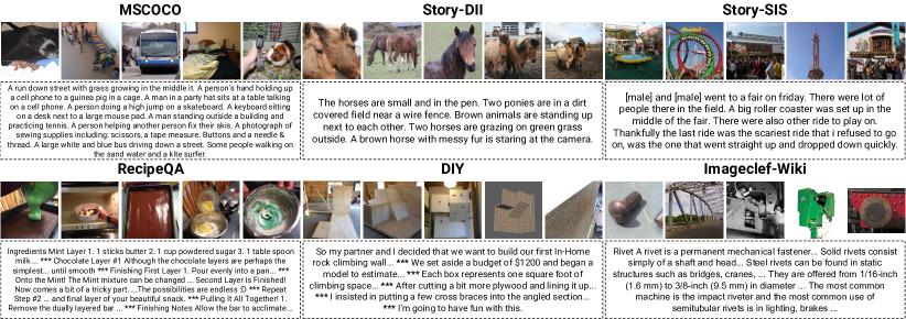
Figure 2: Sample documents from six of our datasets. Image sets and sentence sets may be truncated due to space constraints. The example from Story-DII is harder than is typical, but we include it to illustrate a point regarding image spread made in §4.1. *** denotes text-chunk delimiters present in the original data.

Assignment Problem (AP). We may wish to consider the image-sentence alignment task as a bipartite linear assignment problem (Kuhn, 1955), such that each image/sentence in a document has at most one association. Each time we compute ${\rm sim}(S,V)$ in the forward pass of our models, we solve the integer programming problem of maximizing $\sum_{i,j}\widehat{M}_{ij}x_{ij}$ subject to the constraints:

$${\color[rgb]{1,0,0}\forall i,\sum_{j}x_{ij}\leq 1;}\,{\color[rgb]{0,0,1}\forall j,\sum_{i}x_{ij}\leq 1;}\,{\color[rgb]{1,0,1}\forall i,j,x_{ij}\in\{0,1\}.}$$

Despite involving a discrete optimization step, the model remains fully differentiable. Our forward pass uses tensorflow’s python interface, tf.py_func, and the lapjv implementation of the JV algorithm Jonker and Volgenant (1987) to solve the integer program itself. Given the solution $x^{*}_{ij}$, we compute (and backpropagate gradients through) the similarity function ${\rm sim}(S,V)=\left(\sum_{i,j}M_{ij}x^{*}_{ij}\right)/r$ where $r$ is the number of non-zero $x^{*}_{ij}$. Should we want to impose an upper bound $k$ on the number of links, we can add the following additional constraint: $\sum_{i,j}x_{ij}\leq k(S,V)$. For example, one could set $k(S,V)=\frac{1}{2}\min(|S|,|V|)$.

The JV algorithm’s runtime is $O(\max(n,m)^{3})$, and each positive example requires computing similarities for the positive case and the $2b$ negative samples from Eq. 1, for a per-example runtime of $O(b\cdot\max(n,m)^{3})$. Fortunately, lapjv is highly optimized, so despite solving many integer programs, AP often runs faster than DC.

3.3 Baselines

We construct two baseline similarity functions, as we are not aware of existing models that directly address our task in an unsupervised fashion.

Object Detection. For each image in the document, we use DenseNet169 (Huang et al., 2017) to find its $K$ most probable ImageNet classes (e.g., “stingray”), and represent the image as the average of the word2vec embeddings of those $K$ labels. We represent each sentence in a document as the mean word2vec embedding of its words. To form the strongest possible baseline, we compute the cosine similarity between all sentence-image pairs to form $\widehat{M}$ for $K\in\{1...20\}$ and report the variant with the best post-hoc performance on the test set.

NoStruct. The similarity functions described in §3.2 rely on document-level, structural information, i.e., for a single image in a document, the other images in a document affect the overall similarity (and vice versa for sentences). However, this structural information may not be worth incorporating. Thus, we train a baseline that solely relies on single image/single sentence co-occurrence statistics. At training time, we randomly sample a single image and a single sentence from a document, compute the cosine similarity of their vector representations, and treat that value as the document similarity. While the randomly sampled image/sentence will not truly correspond for every sample, we still expect this baseline to produce above-random results when averaged over many iterations, as true correspondences have some (low) probability of being sampled.

4 Experiments on Crowdlabeled Data

Our first set of experiments uses four pre-existing datasets created by asking crowdworkers to add sentence-long textual descriptions to images in a collection. Image-sentence alignments are therefore known by construction. We do not use these labels at training time: gold-standard alignments are only used at evaluation time to compare performance between algorithms. Statistics of these datasets are given in the top half of Table 1, and example documents are given in Figure 2. Each crowdlabeled dataset is constructed to address a different question about our learning setting.

Q: Is this task even possible? Test: MSCOCO. MSCOCO (Lin et al., 2014) was created by crowdsourced manual captioning of single images. We construct “documents” from this data by first randomly aggregating five image-caption pairs. We then add five “distractor” images with no captions and five “distractor” captions with no images. Thus, a non-distractor image truly corresponds to the single caption that was written about it, and not to the other 9 captions in the document. There are a total of 10 images/sentences per document, and 5 ground-truth image-sentence links. A priori, we expect this to be the easiest setting for within-document disambiguation because mismatched images and sentences are completely independent.

Q: What if the images/sentences within a document are similar? Test: Story-DII. Huang et al. (2016) asked crowdworkers to collect subsets of images contained in the same Flickr album (Thomee et al., 2016) that could be arranged into a visual story. In the Story-DII (= “descriptions in isolation”) case, (possibly different) crowdworkers subsequently captioned the images, but only saw each image in isolation. We construct a set of documents from Story-DII so that each contains five images and five sentences. Because images come from the same album, images and captions in our Story-DII “documents” are more similar to each other than those in our MSCOCO “documents.”

Q: What if the sentences are cohesive and refer to each other? Test: Story-SIS. Huang et al. (2016) also presented all the images in a subset from the same Flickr album to crowdworkers simultaneously and asked them to caption the image subsets collectively to form a story (SIS = “story in sequence”). In contrast to Story-DII, the generated sentences are generally not stand-alone descriptions of the corresponding image’s contents, and may, for example, use pronouns to refer to elements from neighboring sentences and images.

Q: What if there are many sentences with no corresponding images? Test: DII-Stress. Because documents often have many sentences that do not directly refer to visual content, we constructed a setting with many more sentences than images. We augment documents from Story-DII with 45 randomly negatively sampled distractor captions. The resulting documents have five images and fifty sentences, where only five sentences truly describe images in the document.

	train/val/test	$n_{i}/m_{i}$	# imgs	density
		(median)	(unique)
MSCOCO	25K/2K/2K	10/10	83K	5%
Story-DII	22K/3K/3K	5/5	47K	20%
Story-SIS	37K/5K/5K	5/5	76K	20%
DII-Stress	22K/3K/3K	50/5	47K	2%
DIY	7K/1K/1K	15/16	154K	8%
RQA	7K/1K/1K	6/8	88K	17%
WIKI	14K/1K/1K	86/5	92K	N/A

Table 1: Dataset statistics: top half = crowdlabeled datasets; bottom half = organically-multimodal datasets. Density measures the sparsity of the ground truth graph as the number of ground-truth edges divided by the number of possible edges.

	MSCOCO		Story-DII		Story-SIS		DII-Stress
	${\scriptstyle\sf{AUC}}$	p@1/p@5	${\scriptstyle\sf{AUC}}$	p@1/p@5	${\scriptstyle\sf{AUC}}$	p@1/p@5	${\scriptstyle\sf{AUC}}$	p@1/p@5
Random	49.7	5.0/4.6	49.4	19.5/19.2	50.0	19.4/19.7	50.0	2.0/2.0
Obj Detect	89.5	67.7/45.9	65.3	50.2/35.2	58.4	40.8/28.6	76.9	25.7/17.5
NoStruct	87.5	50.6/34.6	76.6	60.1/46.2	64.9	43.2/33.7	84.2	21.4/15.6
DC	98.9	93.6/80.1	82.8	71.5/55.5	68.8	51.8/38.6	94.9	64.6/44.8
TK	98.9	93.9/80.1	82.9	71.4/55.5	68.8	50.9/38.7	95.2	65.6/45.3
$\Lsh$ + $\frac{1}{2}k$	99.0	95.0/81.1	82.0	72.6/54.9	67.6	51.9/38.0	94.7	64.0/43.7
AP	98.7	91.0/78.0	82.6	70.5/55.0	68.5	50.5/38.3	95.3	65.5/45.7
$\Lsh$ + $\frac{1}{2}k$	98.9	93.9/80.4	81.6	72.4/54.4	67.4	52.1/37.7	94.5	65.0/43.4

Table 2: Results for crowdlabeled datasets (similar results for other settings are included in the supplementary material). Values are bolded if they are within 1% of the best-in-column performance.

Number of Epochs

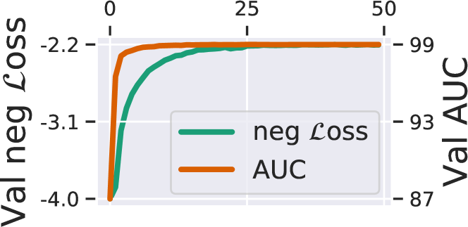
(a) MSCOCO

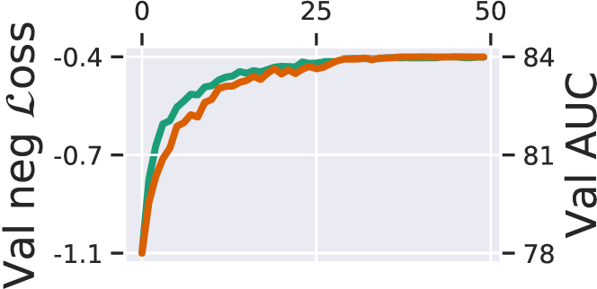
(b) Story-DII

Figure 3: Inter-document objective (AP, $b=10$) and intra-document ${\scriptstyle\sf{AUC}}$ increase together during training.

Experiment Protocols. We conduct our evaluations over a single randomly sampled train/dev/test split. For image features, we extract the pre-classification layer of DenseNet169 Huang et al. (2017) pretrained on the ImageNet Russakovsky et al. (2015) classification task, unless otherwise specified. We train with Adam Kingma and Ba (2014) using a starting learning rate of .0001 for 50 epochs. We decrease the learning rate by a factor of 5 each time the loss in Eq. 1 over the dev set plateaus for more than 3 epochs. We set $d_{{\rm multi}}=1024$, and apply dropout with $p=.4$. At test time, we use the model checkpoint with the lowest dev error.

4.1 Crowdlabeled-Data Results

We tried all combinations of $b\in\{10,20,30\}$, ${\rm sim}\in\{{\rm DC},{\rm TK},{\rm AP}\}$. For TK and AP we set the maximum link threshold $k$ to $\min(S_{i},V_{i})$ or $\lceil\frac{1}{2}\min(S_{i},V_{i})\rceil$ (denoted $\frac{1}{2}k$ in the results table).

Table 2 shows test-set prediction results for $b=10$ (results for $b\in\{20,30\}$ are similar). The retrieval-style objectives we consider encourage algorithms to learn useful within-document representations, and incorporating a structured similarity is beneficial. All our algorithms outperform the strongest baseline (NoStruct) in all cases, e.g., by at least 10 absolute percentage points in p@1 on Story-DII.

We next show, as a sanity check, that our inter-document training objective function (Eq. 1) corresponds to intra-document prediction performance (the actual function of interest). Figure 3 plots how both functions vary with number of epochs, for two different validation datasets. In general, inter-document performance and intra-document performance rise together during training; for a fixed neural architecture, models better at optimizing the inter-document loss in Eq. 1 also generally produce better intra-document representations.

In addition, we found that i) DC, despite assuming every sentence corresponds to an image, achieves high performance on DII-Stress, even though 90% of its sentences do not correspond to an image; ii) Allowing AP/TK to make fewer connections (i.e., setting $\frac{1}{2}k$) did not result in significant performance changes, even in the MSCOCO case, where the true number of links (5) was the same as the number of links accounted for by AP/TK+$\frac{1}{2}k$; and iii) adding topical cohesion (MSCOCO $\rightarrow$ Story-DII) makes the task more difficult, as does adding textual cohesion (Story-DII $\rightarrow$ Story-SIS).

Models have trouble with the same documents. We calculated ${\scriptstyle\sf{AUC}}$ for each test document individually. The Spearman correlation between these individual-instance ${\scriptstyle\sf{AUC}}$ values is very high: of all pairs in DC/TK/AP, over all crowdlabeled datasets at b=10, DC vs. AP on MSCOCO had the lowest correlation with $\rho=.89$.

Error analysis: content vs. spread. Why are some instances more difficult to solve for all of our algorithms? We consider two hypotheses. The “content” hypothesis is that some concepts are more difficult for algorithms to find multimodal relationships between: “beauty” may be hard to visualize, whereas “dog” is a concrete concept Lu et al. (2008); Berg et al. (2010); Parikh and Grauman (2011); Hessel et al. (2018); Mahajan et al. (2018). The “spread” hypothesis, which we introduce, is that documents with lower diversity among images/sentences may be harder to disambiguate at test time. For example, a document in which all images and all sentences are about horses requires finer-grained distinctions than a document with a horse, a barn, and a tractor. The Story-DII vs. Story-SIS example in Fig. 2 illustrates this contrast.

To quantify the spread of a document, we first extract vector representations of each test image/sentence. We then L2-normalize the vectors and compute the mean squared distance to their centroid; higher “spread” values indicate that a document’s sentences/images are more diverse. To quantify the content of a document, for simplicity, we mean-pool the image/sentence representations and reduce to 20 dimensions with PCA.

We first compute an OLS regression of image spread + text spread on test ${\scriptstyle\sf{AUC}}$ scores for Story-DII/Story-SIS/DII-Stress for AP with $b=10$: 42/23/16% respectively (F-test $p\ll.01$) of the variance in ${\scriptstyle\sf{AUC}}$ can be explained by the spread hypothesis alone. In general, documents with less diverse content are harder, with image spread explaining more variance than text spread. When adding in the image+text content features, the proportion of ${\scriptstyle\sf{AUC}}$ variance explained increases to 52/35/38%; thus, for these datasets, both the “content” and “spread” hypotheses independently explain document difficulty, though the relative importance of each varies across datasets.

5 Experiments on RQA and DIY

The previous datasets had captions added by crowdworkers for the explicit purpose of aiding research on grounding: for MSCOCO, annotators providing image captions were explicitly instructed to provide literal descriptions and “not describe what a person might say” Chen et al. (2015). The manner in which users interact with multimodal content “in the wild” significantly differs from crowdlabeled data: Marsh and Domas White’s (2003) 49-element taxonomy of multimodal relationships (e.g., “decorate”, “reiterate”, “humanize”) observed in 45 web documents highlights the diversity of possible image-text relationships.

We thus consider two datasets (one of which we release ourselves) of organically-multimodal documents scraped from web data, where the original authors created or selected both images and sentences. Statistics of these datasets are given in the bottom half of Table 1.

	RQA		DIY
	${\scriptstyle\sf{AUC}}$	p@1/p@5	${\scriptstyle\sf{AUC}}$	p@1/p@5
Random	49.4	17.8/16.7	49.8	6.3/6.8
Obj Detect	58.7	25.1/21.5	53.4	17.9/11.8
NoStruct	60.5	33.8/27.0	57.0	13.3/11.8
DC	63.5	38.3/30.6	59.3	20.8/16.1
TK	67.9	44.0/35.8	60.5	21.2/16.0
$\Lsh$ + $\frac{1}{2}k$	68.1	44.5/35.4	56.0	14.1/12.5
AP	69.3	47.3/37.3	61.8	22.5/17.2
$\Lsh$ + $\frac{1}{2}k$	68.7	47.2/36.2	59.4	21.6/15.3

Table 3: Performance on the organically-multimodal data; values within 1% of best-in-column are bolded.

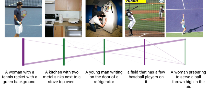
(a) MSCOCO; 97 ${\scriptstyle\sf{AUC}}$, 10 sentences/10 images.

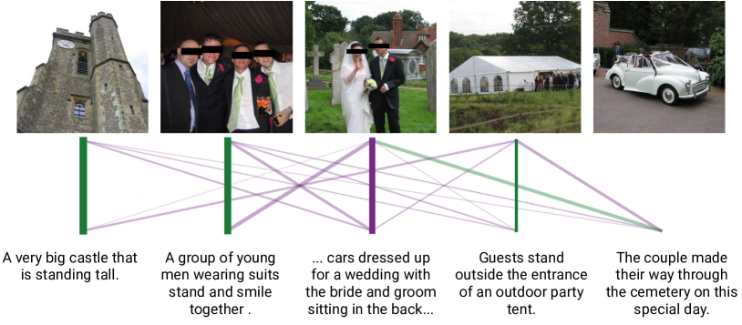
(b) Story-DII; 83 ${\scriptstyle\sf{AUC}}$, 5 sentences/5 images.

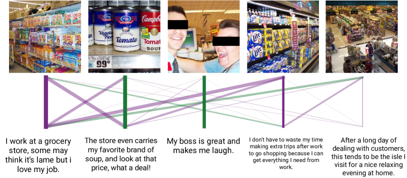
(c) Story-SIS; 70 ${\scriptstyle\sf{AUC}}$, 5 sentences/5 images.

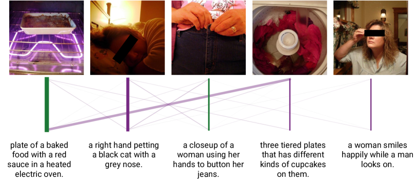
(d) DII-Stress; 94 ${\scriptstyle\sf{AUC}}$, 50 sentences/5 images.

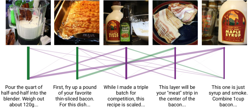
(e) RQA; 70 ${\scriptstyle\sf{AUC}}$, 9 sentences/18 images.

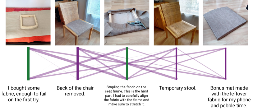
(f) DIY; 62 ${\scriptstyle\sf{AUC}}$, 17 sentences/17 images.

Figure 4: Example test-time graph predictions from AP with $b=10$. Each subfigure gives the top 5 image/sentence predictions per document, in decreasing order of confidence from left to right. Green edges indicate ground-truth pairs; edge widths show the magnitude of edges in $\widehat{M}_{i}$ (only positive weights are shown). Examples are selected to be representative: per-document ${\scriptstyle\sf{AUC}}$ (roughly) matches the average ${\scriptstyle\sf{AUC}}$ achieved on the corresponding dataset.

RQA. RecipeQA Yagcioglu et al. (2018) is a question-answering dataset scraped from instructibles.com consisting of images/descriptions of food preparation steps; we construct documents by treating each recipe step as a sentence. Users of the Instructibles web interface put images and recipe steps in direct correspondence, which gives us a graph for test time evaluation.

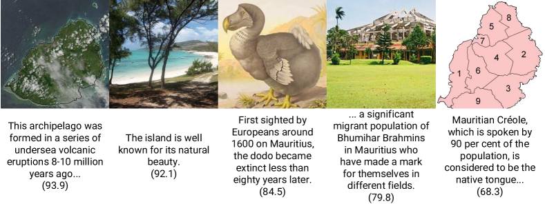
Figure 5: Predicted sentences, with cosine similarities, for images in a 100-sentence ImageCLEF Wikipedia article on Mauritius. The first three predictions are reasonable, the last two are not. The third result is particularly good given that only two sentences mention dodos; for comparison, the object-detection’s choice began “(Mauritian Creole people usually known as ‘Creoles’)”.

DIY (new). We downloaded a sample of 9K Reddit posts made to the community DIY (“do it yourself”). These posts consist of multiple images that users have taken of the progression of their construction projects, e.g., building a rock climbing wall (see Figure 2). Users are encouraged to explicitly annotate individual images with captions, and, for evaluation, we treat a caption written alongside a given image as corresponding to a true link.

We adopt the same experimental protocols as in §4, but increase the maximum sentence token-length from 20 to 50; Table 3 shows the test-set results. In general, the algorithms we introduce again outperform the NoStruct baseline. In contrast to the crowdlabeled experiments, AP (slightly) outperformed the other algorithms. DIY is the most difficult among the datasets we consider.

To see if the algorithms err on the same instances, we again compute the Spearman correlation $\rho$ between test-instance ${\scriptstyle\sf{AUC}}$ scores for DC/TK/AP, for $b=10$. We find greater variation in performance on organically-multimodal compared to crowdlabeled data. For example, on RQA, DC and AP have a $\rho$ of only $.64$. We also repeat the regression on test-instance ${\scriptstyle\sf{AUC}}$ scores introduced in §4.1 with different results; content generally explains more variance than spread, e.g., for AP, for RQA/DIY respectively, only 2/1% is explained by spread alone, but 18/13% is explained by spread+content.

6 Qualitative Exploration

To visualize the within-document prediction for document $i$, we compute $\widehat{M}_{i}$ and solve the linear assignment problem described in §2, taking the edges with highest selected weights to be the most confident. Figure 4 contains example test predictions (along with $\widehat{M}_{i}$) from the datasets with ground-truth annotation. In an effort to provide representative cases, the selected examples have ${\scriptstyle\sf{AUC}}$ scores close to average performance for their corresponding datasets.

The model mostly succeeds at associating literal objects and their descriptions: tennis players in MSCOCO, castles in Story-DII, a stapler in DIY, and bacon in a blender in RQA. Errors are often justifiable. For example, for the MSCOCO document, the chosen caption for a picture of two people playing baseball accurately describes the image, despite it having been written for a different image and thus counting as an error in our quantitative evaluation. Similarly, for RQA, a container of maple syrup is associated with a caption mentioning “syrup”, which seems reasonable even though the recipe’s author did not link that image/sentence.

In other cases, the algorithm struggles with what part of the image to “pay attention” to. In the Story-DII case (Figure 4(b)), the algorithm erroneously (but arguably justifiably) decides to assign a caption about a bride, groom, and a car to a picture of the couple, instead of to a picture of a vehicle.

For more difficult datasets like Story-SIS (Figure 4(c)), the algorithm struggles with ambiguity. For 2/5 sentences that refer to literal objects/actions (soup cans/laughter), the algorithm works well. The remaining 3 captions are general musings about working at a grocery store that could be matched to any of the three remaining images depicting grocery store aisles. DIY is similarly difficult, as many images/sentences could reasonably be assigned to each other.

WIKI. We also constructed a dataset from English sentence-tokenized Wikipedia articles (not including captions) and their associated images from ImageCLEF2010 Popescu et al. (2010). In contrast to RQA and DIY, there are no explicit connections between individual images and individual sentences, so we cannot compute ${\scriptstyle\sf{AUC}}$ or precision, but this corpus represents an important organically-multimodal setting. We follow the same experimental settings as in §4 at training time, but instead of using pre-extracted features, we fine-tune the vision model’s parameters. Examining the predictions of the AP+fine-tuned CNN model trained on WIKI shows many of the model’s predictions to be reasonable. Figure 5 shows the model’s 5 most confident predictions on the 100-sentence Wikipedia article about Mauritius, chosen for its high image/text spread.

7 Additional related work

Our similarity functions are inspired by work in aligning image fragments, such as object bounding boxes, with portions of sentences without explicit labels Karpathy et al. (2014); Karpathy and Fei-Fei (2015); Jiang et al. (2015); Rohrbach et al. (2016); Datta et al. (2019); similar tasks have been addressed in supervised Plummer et al. (2015) and semi-supervised Rohrbach et al. (2016) settings. Our models operate at the larger granularity of entire images/sentences. Integer programs like AP have been used to align visual and textual content in videos, e.g., Bojanowski et al. (2015)

Prior work has addressed the task of identifying objects in single images that are referred to by natural language descriptions Mitchell et al. (2010, 2013); Kazemzadeh et al. (2014); Karpathy et al. (2014); Plummer et al. (2015); Hu et al. (2016b); Rohrbach et al. (2016); Nagaraja et al. (2016); Hu et al. (2016a); Yu et al. (2016); Peyre et al. (2017); Margffoy-Tuay et al. (2018). In general, a supervised approach is taken (Mao et al., 2016; Krishna et al., 2017; Johnson et al., 2017).

Related tasks involving multi-image/multi-sentence data include: generating captions/stories for image streams or videos Park and Kim (2015); Huang et al. (2016); Shin et al. (2016); Liu et al. (2017), sorting aligned (image, caption) pairs into stories Agrawal et al. (2016), image/textual cloze tasks Iyyer et al. (2017); Yagcioglu et al. (2018), augmentation of Wikipedia articles with 3D models Russell et al. (2013), question-answering Kembhavi et al. (2017), and aligning books with their film adaptations Zhu et al. (2015); these tasks are usually supervised, or rely on a search engine.

8 Conclusion and Future Directions

We have demonstrated that a family of models for learning fine-grained image-sentence links within documents can produce good test-time results even if only given access to document-level co-occurrence at training time. Future work could incorporate better models of sequence within document context (Kim et al., 2015; Alikhani and Stone, 2018). While using structured loss functions improved performance, image and sentence representations themselves have no awareness of neighboring images/sentences; this information should prove useful if modeled appropriately.

Acknowledgments. We thank Yoav Artzi, Cristian Danescu-Niculescu-Mizil, Jon Kleinberg, Vlad Niculae, Justine Zhang, the Cornell NLP seminar, the reviewers, and Ondrej Linda, Randy Puttick, Ramin Mehran, and Grant Long of Zillow for helpful comments. We additionally thank the NVidia Corporation for the GPUs used in this study. This material is supported by the U.S. National Science Foundation under grants BIGDATA SES-1741441, 1526155, 1652536, and the Alfred P. Sloan Foundation. Any opinions, findings, and conclusions or recommendations expressed in this material are those of the authors and do not necessarily reflect the views of the sponsors.

References

- Agrawal et al. (2016) Harsh Agrawal, Arjun Chandrasekaran, Dhruv Batra, Devi Parikh, and Mohit Bansal. 2016. Sort story: Sorting jumbled images and captions into stories. In EMNLP.
- Alikhani and Stone (2018) Malihe Alikhani and Matthew Stone. 2018. Exploring coherence in visual explanations. In Multimedia Information Processing and Retrieval.
- Berg et al. (2010) Tamara L Berg, Alexander C Berg, and Jonathan Shih. 2010. Automatic attribute discovery and characterization from noisy web data. In ECCV.
- Bojanowski et al. (2015) Piotr Bojanowski, Rémi Lajugie, Edouard Grave, Francis Bach, Ivan Laptev, Jean Ponce, and Cordelia Schmid. 2015. Weakly-supervised alignment of video with text. In ICCV.
- Chen et al. (2015) Xinlei Chen, Hao Fang, Tsung-Yi Lin, Ramakrishna Vedantam, Saurabh Gupta, Piotr Dollár, and C. Lawrence Zitnick. 2015. Microsoft COCO captions: Data collection and evaluation server. Computing Research Repository, arXiv:1504.00325. Version 2.
- Cho et al. (2014) Kyunghyun Cho, Bart van Merrienboer, Caglar Gulcehre, Dzmitry Bahdanau, Fethi Bougares, Holger Schwenk, and Yoshua Bengio. 2014. Learning phrase representations using RNN encoder–decoder for statistical machine translation. In EMNLP.
- Costa Pereira et al. (2014) Jose Costa Pereira, Emanuele Coviello, Gabriel Doyle, Nikhil Rasiwasia, Gert R. G. Lanckriet, Roger Levy, and Nuno Vasconcelos. 2014. On the role of correlation and abstraction in cross-modal multimedia retrieval. TPAMI.
- Dalal and Triggs (2005) Navneet Dalal and Bill Triggs. 2005. Histograms of oriented gradients for human detection. In CVPR.
- Datta et al. (2019) Samyak Datta, Karan Sikka, Anirban Roy, Karuna Ahuja, Devi Parikh, and Ajay Divakaran. 2019. Align2ground: Weakly supervised phrase grounding guided by image-caption alignment. In ICCV.
- Faghri et al. (2018) Fartash Faghri, David J Fleet, Jamie Ryan Kiros, and Sanja Fidler. 2018. VSE++: Improving visual-semantic embeddings with hard negatives. In British Machine Vision Conference.
- Hessel et al. (2018) Jack Hessel, David Mimno, and Lillian Lee. 2018. Quantifying the visual concreteness of words and topics in multimodal datasets. In NAACL.
- Hodosh et al. (2013) Micah Hodosh, Peter Young, and Julia Hockenmaier. 2013. Framing image description as a ranking task: Data, models and evaluation metrics. Journal of Artificial Intelligence Research.
- Hu et al. (2016a) Ronghang Hu, Marcus Rohrbach, and Trevor Darrell. 2016a. Segmentation from natural language expressions. In ECCV.
- Hu et al. (2016b) Ronghang Hu, Huazhe Xu, Marcus Rohrbach, Jiashi Feng, Kate Saenko, and Trevor Darrell. 2016b. Natural language object retrieval. In CVPR.
- Huang et al. (2017) Gao Huang, Zhuang Liu, Laurens Van Der Maaten, and Kilian Q. Weinberger. 2017. Densely connected convolutional networks. In CVPR.
- Huang et al. (2016) Ting-Hao (Kenneth) Huang, Francis Ferraro, Nasrin Mostafazadeh, Ishan Misra, Aishwarya Agrawal, Jacob Devlin, Ross Girshick, Xiaodong He, Pushmeet Kohli, Dhruv Batra, C. Lawrence Zitnick, Devi Parikh, Lucy Vanderwende, Michel Galley, and Margaret Mitchell. 2016. Visual storytelling. In NAACL.
- Iyyer et al. (2017) Mohit Iyyer, Varun Manjunatha, Anupam Guha, Yogarshi Vyas, Jordan Boyd-Graber, Hal Daumé III, and Larry S. Davis. 2017. The amazing mysteries of the gutter: Drawing inferences between panels in comic book narratives. In CVPR.
- Jiang et al. (2015) Xinyang Jiang, Fei Wu, Xi Li, Zhou Zhao, Weiming Lu, Siliang Tang, and Yueting Zhuang. 2015. Deep compositional cross-modal learning to rank via local-global alignment. In ACM MM.
- Johnson et al. (2017) Justin Johnson, Bharath Hariharan, Laurens van der Maaten, Li Fei-Fei, C. Lawrence Zitnick, and Ross Girshick. 2017. CLEVR: A diagnostic dataset for compositional language and elementary visual reasoning. In CVPR.
- Jonker and Volgenant (1987) Roy Jonker and Anton Volgenant. 1987. A shortest augmenting path algorithm for dense and sparse linear assignment problems. Computing.
- Karpathy and Fei-Fei (2015) Andrej Karpathy and Li Fei-Fei. 2015. Deep visual-semantic alignments for generating image descriptions. In CVPR.
- Karpathy et al. (2014) Andrej Karpathy, Armand Joulin, and Li F Fei-Fei. 2014. Deep fragment embeddings for bidirectional image sentence mapping. In NeurIPS.
- Kazemzadeh et al. (2014) Sahar Kazemzadeh, Vicente Ordonez, Mark Matten, and Tamara Berg. 2014. ReferItGame: Referring to objects in photographs of natural scenes. In EMNLP.
- Kembhavi et al. (2017) Aniruddha Kembhavi, Minjoon Seo, Dustin Schwenk, Jonghyun Choi, Ali Farhadi, and Hannaneh Hajishirzi. 2017. Are you smarter than a sixth grader? Textbook question answering for multimodal machine comprehension. In CVPR.
- Kim et al. (2015) Gunhee Kim, Seungwhan Moon, and Leonid Sigal. 2015. Ranking and retrieval of image sequences from multiple paragraph queries. In CVPR.
- Kingma and Ba (2014) Diederik P. Kingma and Jimmy Ba. 2014. Adam: A method for stochastic optimization. Computing Research Repository, arXiv:1412.6980. Version 5.
- Kiros et al. (2014a) Ryan Kiros, Ruslan Salakhutdinov, and Rich Zemel. 2014a. Multimodal neural language models. In ICML.
- Kiros et al. (2014b) Ryan Kiros, Ruslan Salakhutdinov, and Richard S. Zemel. 2014b. Unifying visual-semantic embeddings with multimodal neural language models. In NeurIPS Deep Leaning Workshop.
- Krishna et al. (2017) Ranjay Krishna, Yuke Zhu, Oliver Groth, Justin Johnson, Kenji Hata, Joshua Kravitz, Stephanie Chen, Yannis Kalantidis, Li-Jia Li, David Ayman Shamma, Michael Bernstein, and Li Fei-Fei. 2017. Visual genome: Connecting language and vision using crowdsourced dense image annotations. International Journal of Computer Vision.
- Kuhn (1955) Harold W. Kuhn. 1955. The Hungarian method for the assignment problem. Naval research logistics quarterly.
- Li et al. (2015) Jiwei Li, Minh-Thang Luong, and Dan Jurafsky. 2015. A hierarchical neural autoencoder for paragraphs and documents. In ACL.
- Lin et al. (2014) Tsung-Yi Lin, Michael Maire, Serge Belongie, James Hays, Pietro Perona, Deva Ramanan, Piotr Dollár, and C. Lawrence Zitnick. 2014. Microsoft COCO: Common objects in context. In ECCV.
- Liu et al. (2017) Yu Liu, Jianlong Fu, Tao Mei, and Chang Wen Chen. 2017. Let your photos talk: Generating narrative paragraph for photo stream via bidirectional attention recurrent neural networks. In AAAI.
- Lu et al. (2008) Yijuan Lu, Lei Zhang, Qi Tian, and Wei-Ying Ma. 2008. What are the high-level concepts with small semantic gaps? In CVPR.
- Mahajan et al. (2018) Dhruv Mahajan, Ross Girshick, Vignesh Ramanathan, Kaiming He, Manohar Paluri, Yixuan Li, Ashwin Bharambe, and Laurens van der Maaten. 2018. Exploring the limits of weakly supervised pretraining. In ECCV.
- Mao et al. (2016) Junhua Mao, Jonathan Huang, Alexander Toshev, Oana Camburu, Alan L Yuille, and Kevin Murphy. 2016. Generation and comprehension of unambiguous object descriptions. In CVPR.
- Margffoy-Tuay et al. (2018) Edgar Margffoy-Tuay, Juan C Pérez, Emilio Botero, and Pablo Arbeláez. 2018. Dynamic multimodal instance segmentation guided by natural language queries. In ECCV.
- Marsh and Domas White (2003) Emily E. Marsh and Marilyn Domas White. 2003. A taxonomy of relationships between images and text. Journal of Documentation.
- Menon and Elkan (2011) Aditya Krishna Menon and Charles Elkan. 2011. Link prediction via matrix factorization. In ECML PKDD.
- Mikolov et al. (2013) Tomas Mikolov, Ilya Sutskever, Kai Chen, Greg S. Corrado, and Jeff Dean. 2013. Distributed representations of words and phrases and their compositionality. In NeurIPS.
- Mitchell et al. (2010) Margaret Mitchell, Kees van Deemter, and Ehud Reiter. 2010. Natural reference to objects in a visual domain. In International Natural Language Generation Conference.
- Mitchell et al. (2013) Margaret Mitchell, Ehud Reiter, and Kees Van Deemter. 2013. Typicality and object reference. In Proceedings of the Annual Meeting of the Cognitive Science Society.
- Nagaraja et al. (2016) Varun K. Nagaraja, Vlad I. Morariu, and Larry S. Davis. 2016. Modeling context between objects for referring expression understanding. In ECCV.
- Parikh and Grauman (2011) Devi Parikh and Kristen Grauman. 2011. Interactively building a discriminative vocabulary of nameable attributes. In CVPR.
- Park and Kim (2015) Cesc C. Park and Gunhee Kim. 2015. Expressing an image stream with a sequence of natural sentences. In NeurIPS.
- Peyre et al. (2017) Julia Peyre, Josef Sivic, Ivan Laptev, and Cordelia Schmid. 2017. Weakly-supervised learning of visual relations. In ICCV.
- Plummer et al. (2015) Bryan A. Plummer, Liwei Wang, Chris M. Cervantes, Juan C. Caicedo, Julia Hockenmaier, and Svetlana Lazebnik. 2015. Flickr30k entities: Collecting region-to-phrase correspondences for richer image-to-sentence models. In ICCV.
- Popescu et al. (2010) Adrian Popescu, Theodora Tsikrika, and Jana Kludas. 2010. Overview of the Wikipedia retrieval task at ImageCLEF 2010. In CLEF.
- Rasiwasia et al. (2010) Nikhil Rasiwasia, Jose Costa Pereira, Emanuele Coviello, Gabriel Doyle, Gert R. G. Lanckriet, Roger Levy, and Nuno Vasconcelos. 2010. A new approach to cross-modal multimedia retrieval. In ACM MM.
- Rohrbach et al. (2016) Anna Rohrbach, Marcus Rohrbach, Ronghang Hu, Trevor Darrell, and Bernt Schiele. 2016. Grounding of textual phrases in images by reconstruction. In ECCV.
- Russakovsky et al. (2015) Olga Russakovsky, Jia Deng, Hao Su, Jonathan Krause, Sanjeev Satheesh, Sean Ma, Zhiheng Huang, Andrej Karpathy, Aditya Khosla, Michael Bernstein, Alexander C. Berg, and Li Fei-Fei. 2015. ImageNet large scale visual recognition challenge. International Journal of Computer Vision.
- Russell et al. (2013) Bryan C. Russell, Ricardo Martin-Brualla, Daniel J. Butler, Steven M. Seitz, and Luke Zettlemoyer. 2013. 3D Wikipedia: Using online text to automatically label and navigate reconstructed geometry. ACM Transactions on Graphics.
- Schroff et al. (2015) Florian Schroff, Dmitry Kalenichenko, and James Philbin. 2015. Facenet: A unified embedding for face recognition and clustering. In CVPR.
- Sharif Razavian et al. (2014) Ali Sharif Razavian, Hossein Azizpour, Josephine Sullivan, and Stefan Carlsson. 2014. CNN features off-the-shelf: an astounding baseline for recognition. In CVPR.
- Shin et al. (2016) Andrew Shin, Katsunori Ohnishi, and Tatsuya Harada. 2016. Beyond caption to narrative: Video captioning with multiple sentences. In International Conference on Image Processing (ICIP).
- Thomee et al. (2016) Bart Thomee, David A. Shamma, Gerald Friedland, Benjamin Elizalde, Karl Ni, Douglas Poland, Damian Borth, and Li-Jia Li. 2016. YFCC100M: the new data in multimedia research. Communications of the ACM.
- Volgenant (2004) Anton Volgenant. 2004. Solving the k-cardinality assignment problem by transformation. European Journal of Operational Research.
- Wu et al. (2017) Shaomei Wu, Jeffrey Wieland, Omid Farivar, and Julie Schiller. 2017. Automatic alt-text: Computer-generated image descriptions for blind users on a social network service. In CSCW.
- Yagcioglu et al. (2018) Semih Yagcioglu, Aykut Erdem, Erkut Erdem, and Nazli Ikizler-Cinbis. 2018. RecipeQA: A challenge dataset for multimodal comprehension of cooking recipes. In EMNLP.
- Yang et al. (2016) Zichao Yang, Diyi Yang, Chris Dyer, Xiaodong He, Alex Smola, and Eduard Hovy. 2016. Hierarchical attention networks for document classification. In NAACL.
- Yu et al. (2016) Licheng Yu, Patrick Poirson, Shan Yang, Alexander C. Berg, and Tamara L. Berg. 2016. Modeling context in referring expressions. In ECCV.
- Zhu et al. (2015) Yukun Zhu, Ryan Kiros, Rich Zemel, Ruslan Salakhutdinov, Raquel Urtasun, Antonio Torralba, and Sanja Fidler. 2015. Aligning books and movies: Towards story-like visual explanations by watching movies and reading books. In ICCV.
- Zoph et al. (2018) Barret Zoph, Vijay Vasudevan, Jonathon Shlens, and Quoc V. Le. 2018. Learning transferable architectures for scalable image recognition. In CVPR.