Cryo-Electron Microscopy Image Analysis Using Multi-Frequency Vector Diffusion Maps

Abstract

Cryo-electron microscopy (EM) single particle reconstruction is an entirely general technique for 3D structure determination of macromolecular complexes. However, because the images are taken at low electron dose, it is extremely hard to visualize the individual particle with low contrast and high noise level. In this paper, we propose a novel approach called multi-frequency vector diffusion maps (MFVDM) to improve the efficiency and accuracy of cryo-EM 2D image classification and denoising. This framework incorporates different irreducible representations of the estimated alignment between similar images. In addition, we propose a graph filtering scheme to denoise the images using the eigenvalues and eigenvectors of the MFVDM matrices. Through both simulated and publicly available real data, we demonstrate that our proposed method is efficient and robust to noise compared with the state-of-the-art cryo-EM 2D class averaging and image restoration algorithms.

I Introduction

Scientific breakthroughs often build upon successful visualization of objects invisible to the human eye. The 2017 Nobel Prize in Chemistry was awarded for the development of cryo-electron microscopy (cryo-EM) that allows us to image biomolecules in their native functional states at high resolution. This method has moved biochemistry into a new era. In cryo-EM experiments, the purified protein particles are distributed evenly within the special sample grid holes assuming a variety of random orientations (see Fig. 1). The single particle images are boxed out during the particle picking step [12, 8]. Despite the recent progress, there still remain a lot of challenges for the current computational framework of cryo-EM single particle reconstruction (SPR). For example, in its present form, the methodology still cannot resolve high resolution structures of small particles with molecular weights below 50kDa due to low contrast and signal-to-noise ratio (SNR) [27].

Figure 1: Illustration of image formation in cryo-EM: The electron beam projects the randomly oriented particles. The projection image is modulated by the contrast transfer function (CTF) and corrupted by noise with extremely low SNR.

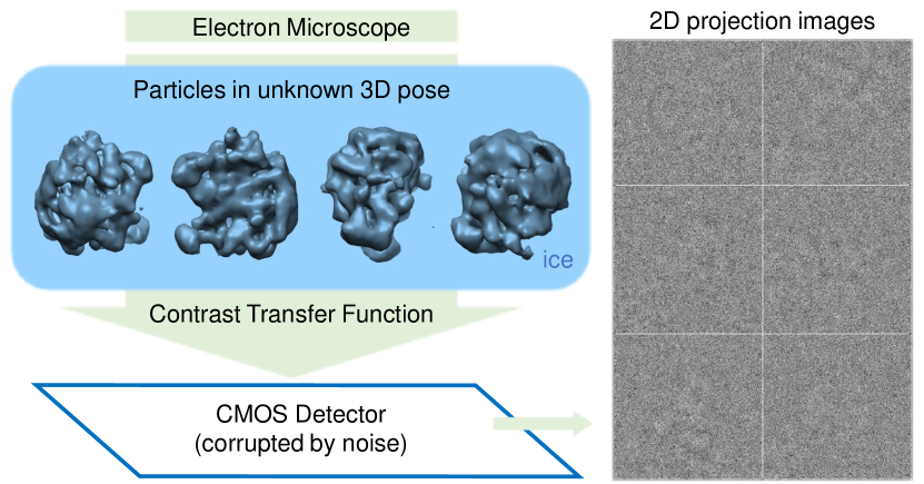
To improve the image quality, a crucial step is the alignment and averaging of the 2D projection images, a procedure known as “2D class averaging.” The 2D analysis of cryo-EM data is used to assess the data quality. They can be used for direct observation to look for heterogeneity, discover symmetry, and separate particles into subgroups for additional analysis. Better denoising also increases the diversity of the selected particle views during particle picking, which is crucial for 3D reconstruction. The denoised images are used for common-lines based 3D ab initio reconstruction [34]. A good initial model reduces the number of refinement iterations and leads to a better reconstruction [40]. Alternative 3D ab initio modeling method uses higher-order moments of the 2D images, such as sample mean, covariance, and triple correlation [9]. Moment estimation is sensitive to noise, therefore better image denoising is crucial for moment based 3D reconstruction. Therefore, it is important to have fast and accurate algorithms for the 2D analysis and denoising.

Many existing cryo-EM single particle reconstruction software packages [22, 4, 31] contain algorithms for 2D class averaging. Most common methods use K-means clustering with iterative rotational alignment and clustering. On the other hand, the ASPIRE class averaging pipeline in [40] performs robust rotational invaraint nearest neighbor search and alignment estimation. It uses steerable principal component analysis (sPCA) to efficiently denoise the large image dataset and uses rotationally invariant features to identify images of similar views. For extremely noisy images, the initial nearest neighbor classification has many outliers and it uses vector diffusion maps (VDM) [30, 29] to further improve the nearest neighbor classification by taking into account the consistency of in-plane rotations along multiple paths that connect neighboring images through their common neighbors. The improved nearest neighbors are aligned and averaged to form class averaged images that enjoy higher SNR. However, VDM might fail at lower SNRs and generating class averages by rotational and shift alignment is time consuming and prone to interpolation error.

In this paper, we introduce a new algorithm called multi-frequency vector diffusion maps (MFVDM) to improve the efficiency and accuracy of cryo-EM 2D image classification and denoising. Based on the initial nearest neighbor identification and alignment, we find including different irreproducible representations of $\mathrm{SO}(2)$ can improve the nearest neighbor classification and alignment estimation. To denoise the images, we use the eigenvalues and eigenvectors of the MFVDM matrices to filter the Fourier-Bessel expansion coefficients of the images and reconstruct the images from the denoised expansion coefficients. To demonstrate our method, we perform comparions with the state-of-the-art algorithms for denoising on two real experimental datasets and simulated datasets at different SNRs.

II Related Work

In the following we review the cryo-EM 2D class averaging and denoising methods. Traditional 2D class averging uses unsupervised classification methods, such as K-means clustering and reference-free alignment [5]. However, since the images can be in-plane rotated, they cannot be aligned well without being first separated into distinct classes. On the other hand, it is hard to separate classes when the images are not aligned well [23]. This leads to a ‘chicken and agg’ problem and approaches that iterate between alginment and classification [5] aim to solve it, including maximum-likelihood (ML) estimation [26, 24, 21, 16] and the neural network for kernel probability density estimator self-organizing map (KerDenSOM) [19]. These methods share a drawback of the high sensitivity to initialization. Therefore, to avoid this, [40] introduced rotationally invariant features to identify nearest neighbors and the corresponding alignments. It then uses a nonlinear dimensionality reduction method, VDM [29], to improve the nearest neighbor search. Images are denoised by a weighted average of their aligned nearest neighbors.

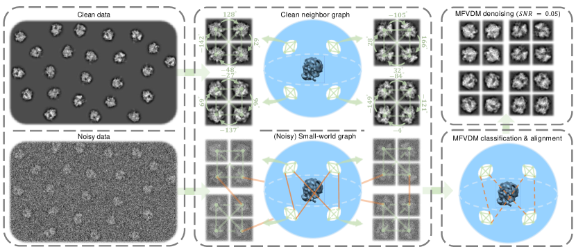
Another type of approaches aims to denoise EM images without 2D classification and averaging and contains two main methods: (1) steerable PCA (sPCA) [39, 38] and (2) covariance Wiener filtering (CWF) [1]. SPCA computes the covariance matrices using the truncated expansion coefficients of the noisy images on steerable basis [38, 10] and uses a Wiener-type filtering to denoise the coefficients. For applications to real cryo-EM images, which are convolved by the point spread function of the electron microscope lens, it requires a data preprocessing step “phase flipping” [20] and does not correct for the phase amplitudes. The second method CWF improves the sPCA by estimating the mean and covariance matrix of the clean data without the lens effect, followed by denoising and deconvolution to correct the Fourier phases and amplitudes of the images. However, neither sPCA nor CWF take into account the geometric structure of the projection images as illustrated in Fig. 3.

Recently, steerable graph Laplacian (SGL) [11] uses a kernel matrix defined on pairs of images including all rotated versions. The eigenvectors of the kernel matrix correpsond to steerable manifold harmonics on the group invariant data manifold. The denoising step uses the truncated global basis to filter the steerable coefficients of the EM images. By taking into account of the nonlinear geometric structure of the data, it improves the denoising performance compared to sPCA. The assumption that the data lie close to a low dimensional manifold was widely used in natural image analysis and computer vision problems. Various global and local filtering have been proposed [32, 2, 36, 6, 25, 18, 37, 3] for image denoising, inpainting, and super-resolution.

Figure 2: Simulated 70S ribosome projections images: (a) Clean projection images. (b) Clean images altered by CTFs. (c) to (e) Images contaminated by additive white Gaussian noise at $\text{SNR}=0.05,0.02,0.01$.

III Methods

Figure 3: Illustration of MFVDM pipeline: Left: Noisy (clean) data samples of a single particle are collected. Middle: The distance $d_{\mathrm{RID}}$ defines a neighborhood graph (clean data) and a small world graph (noisy data) on the unit 2-sphere. Among local neighborhood images, the alignments are consistent for clean data.Right: Using multiple frequency representation, MFVDM is able to remove shortcuts (orange dash lines) and improve the alignment accuracy, then graph filters are used for denoising.

III-A Image Formation Model and Geometry

In cryo-EM single particle experiments, each protein sample is embedded in a thin ice layer at an unknown orientation characterized by a $3\times 3$ orthogonal matrix $R\in\text{SO(3)}$, ($R=[R^{1},R^{2},R^{3}]$). The single particle image $I$ is formed as the X-ray transform of the underlying 3D electron density of the macromolecule. Excluding the contribution of noise, the intensity $I(x,y)$ of the pixel located at $(x,y)$ in the image plane corresponds to the line integral, $I(x,y)=\int\limits_{-\infty}^{\infty}\phi(xR^{1}+yR^{2}+zR^{3})dz$, where $\phi$ is an unknown 3D volume in a fixed coordinate system. For the image $I$, the matrix $R$ can be divided into two parts: (1) the last column $R^{3}$ represents the viewing direction $v=R^{3}$ and uniquely defines a point on a 2-dimensional quotient manifold $\mathcal{M}=\mathrm{SO}(3)/\mathrm{SO}(2)$ (2-dimensional unit sphere) for a generic volume without symmetry; (2) the first two columns of $R$, namely $R^{1}$ and $R^{2}$, form a basis of the tangent plane $T_{I}\mathcal{M}$ and they correspond to the $x,y$ coordinates in the 2D projection image.

The image is corrupted by two phenomena: a contrast transfer function (CTF) [5] and noise. The CTF is analogous to the effects of defocus in a conventional light camera. It modulates the phase amplitudes and flips the signs of the phases in the Fourier domain, which leads to a systematic alteration of the image data (see Figs. 2(a) and 2(b)). The parameters for CTFs are assumed to be known or estimated through standard tools. A simple CTF correction method that does not affect the noise statistics is called phase flipping [20], which corrects the sign of the phases, but not its ampltitude. In our framework, we preprocess the raw images by phase flipping.

For noisy particle images (see Fig. 2(c)), 2D class averaging is an important step to denoise and check the quality of the dataset. It first identifies images with similar views and registers those images by in-plane rotation and shifts. In this paper, we assume that the particles are well centered, and later in the experimental results, we show that the algorithms are robust to small shifts.

For a pair of images $I_{i}$ and $I_{j}$, it is natural to use the rotational invariant distance (RID) $d_{\mathrm{RID}}(i,j)$ to identify images of similar views,

$$d_{\mathrm{RID}}(i,j)=\min_{\alpha\in[0,2\pi)}\left\|I_{i}-\mathcal{R}_{\alpha}I_{j}\right\|,$$ (1)

where $\mathcal{R}_{\alpha}$ is an operator that rotates image $I_{j}$ counter-clockwise by an angle $\alpha$. The associated optimal in-plane rotation alignment is denoted by $\alpha_{ij}$. The underlying alignment angle for images of similar views is determined by $R_{i}$ and $R_{j}$ according to [40, Eqs. (4) and (5)]. The vertices on the blue spheres in Fig. 3 depict the viewing directions. In the noiseless case, small $d_{\mathrm{RID}}$ indicates close viewing directions. Therefore, connecting image pairs with small $d_{\mathrm{RID}}$ form a neighborhood graph on the sphere as shown in the upper middle panel in Fig. 3. However, when the images are extremely noisy, noise aligns well instead of the underlying signals. This results in connecting images of distant views (see the shortcut red edges in the lower middle panel of Fig. 3) and error in the estimation of $\alpha_{ij}$.

To address these challenges, we first use the filtered sPCA coefficients of the images [38] to compute $d_{\mathrm{RID}}$ and $\alpha_{ij}$, which can withstand certain level of noise. Furthermore, in the following subsections, we introduce a graph based method to robustly learn the nonlinear geometrical structure of the image data. The new pipeline combines multiple irreducible representations of the compact alignment group with a random walk executed on a graph where nodes correspond to images and edges denote connections. We then use the learned basis of the manifold to improve nearest neighbor search, alignment, denoising, and deconvolution.

III-B Multi-Frequency Vector Diffusion Maps

For clean projection images, since the viewing directions of the images lie on a 2-sphere, by using $d_{\mathrm{RID}}$, we are able to build a local neighborhood graph $(V,E)$ over the sphere with the nodes $V$ representing the viewing directions and the edges $E$ connecting images of similar views, i.e., $(i,j)\in E$ indicates $\langle v_{i},v_{j}\rangle\approx 1$. All the views of similar images are in a small spherical cap (see the upper middel panel of Fig. 3). In addition, the rotational alignment has cycle consistency among the neighbors, i.e., summing over angles along the cycles will be close to $0\mod 2\pi$.

Based on this graph structure for $n$ images, we build a class of $n\times n$ Hermitian matrices $W_{k}$, for $k=0,1,\dots,\tilde{k}$,

$$W_{k}(i,j)=\begin{cases}e^{\imath k\alpha_{ij}}&(i,j)\in E,\\ 0&(i,j)\notin E,\end{cases}$$ (2)

where $\alpha_{ij}=-\alpha_{ji}$. The degree of each node $\deg(i)=\sum_{j:(i,j)\in E}1$. We define a diagonal matrix $D$ of the same size as $W_{k}$ with $D(i,i)=\deg(i)$. Then the matrix $S_{k}=D^{-1}W_{k}$ is applied to vectors $u$ in the complex plane, which can be viewed as an averaging operator for the tangent vector fields, since

$$(S_{k}u)(i)=\frac{1}{\deg(i)}\sum_{j:(i,j)\in E}e^{\imath k\alpha_{ij}}u(j).$$ (3)

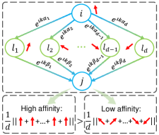
The operator $S_{k}$ transports vectors from the tangent spaces $T_{I_{j}}\mathcal{M}$ to $T_{I_{i}}\mathcal{M}$, for all nearest neighbor $j$, and then averages the transported vectors in $T_{I_{i}}\mathcal{M}$ (see Fig. 4a).

Input: Nearest neighbors list and alignment angles for noisy cryo-EM images from initial classification in [40]

Output: $s$-nearest neighbors for each image and the corresponding optimal alignments $\hat{\alpha}_{ij}$, for $(i,j)\in E$

1 for $k=1,\dots,\tilde{k}$ do

2       Construct the normalized affinity matrix $\widetilde{W}_{k}$ according to Eqs. (2) and (4)

3       Compute the largest $m$ eigenvalues $\lambda^{(k)}_{1}\geq\lambda^{(k)}_{2},\geq,\dots,\geq\lambda^{(k)}_{m}$ of $\widetilde{W}_{k}$ and the corresponding eigenvectors $\{u^{(k)}_{l}\}_{l=1}^{m}$

4       Compute the truncated MFVDM embedding $V^{(k)}_{t,m}$ according to Eq. (6)

5      

6 end for

7Compute the normalized affinity using Eq. (7)

8 Identify $s$ nearest neighbors for each data point

Compute $\hat{\alpha}_{ij}$ for nearest neighbor pairs using Eq. (9)

Algorithm 1 MFVDM nearest neighbor search and alignment

When the images are noisy, the evaluation of $d_{\mathrm{RID}}$ is not accurate and creates shortcut edges, resulting in a small world graph [35] (see lower middle panel of Fig. 3) and leads to poor class average process. To address this problem, note the rotational alignment consistency breaks along the shortcut edges, i.e., if $(i,j)\in E$ is a shortcut, the transportations on different paths between $(i,j)$ are inconsistent (see Fig. 4a). Therefore, we define the affinity between $(i,j)$ by taking into account the consistency of transporting the vectors rotated at different angular frequencies $k$ along the paths with length $2t$, as $\sum_{k=1}^{\tilde{k}}|S^{2t}_{k}(i,j)|^{2}$. Since $S_{k}$ is similar to the symmetric matrix $\widetilde{W}_{k}$,

$$\widetilde{W}_{k}=D_{0}^{-1/2}W_{k}D_{0}^{-1/2},$$ (4)

we can quantify the consistency by computing $\sum_{k=1}^{\tilde{k}}|\widetilde{W}_{k}^{2t}(i,j)|^{2}$. Since $\widetilde{W}_{k}$ is Hermitian, it has real eigenvalues $\{\lambda^{(k)}_{l}\}_{l=1}^{n}$ in descending order and the associated eigenvectors $\{u^{(k)}_{l}\}_{l=1}^{n}$. With the MFVDM mapping defined as

$$V^{(k)}_{t}:i\mapsto\left((\lambda^{(k)}_{l}\lambda^{(k)}_{r})^{t}\langle u^{(k)}_{l}(i),u^{(k)}_{r}(i)\rangle\right)_{l,r=1}^{n},$$ (5)

we have $\left|\widetilde{W}_{k}^{2t}(i,j)\right|^{2}=\left\langle V^{(k)}_{t}(i),V^{(k)}_{t}(j)\right\rangle$ for $k=1,\dots,\tilde{k}$. Through the nonlinear-embedding in (5), the similarity of two images can be evaluated by the inner product of the embedded vectors. VDM [29] is a special case of MFVDM with $\tilde{k}=1$. It was shown in [29] that the VDM can be well approximated by using only the few largest eigenvalues and their corresponding eigenvectors. Similarly, we truncate MFVDM mapping as

$$V^{(k)}_{t,m}:i\mapsto\left((\lambda^{(k)}_{l}\lambda^{(k)}_{r})^{t}\langle u^{(k)}_{l}(i),u^{(k)}_{r}(i)\rangle\right)_{l,r=1}^{m},$$ (6)

with $m<n$. When $t$ is small and $m$ and $\tilde{k}$ are chosen properly [14], the embedding is able to preserve the topological structure of the underlying data manifold and is robust to noise perturbation.

Nearest Neighbor Search: Based on the truncated mapping, we identify nearest neighbors by the normalized affinity $A$ defined as

$$A(i,j)=\sum_{k=1}^{\tilde{k}}\left\langle\frac{V^{(k)}_{t,m}(i)}{\|V_{t,m}^{(k)}(i)\|},\frac{V^{(k)}_{t,m}(j)}{\|V_{t,m}^{(k)}(j)\|}\right\rangle.$$ (7)

Since we take into account various irreducible representations of $\mathrm{SO}(2)$ and the consistency of the corresponding transformations over the graph, this new affinity in Eq. (7) is able to avoid shortcuts, and is more robust to noise compared to VDM (see Fig. 6).

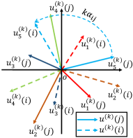
Rotational Alignment: To estimate the in-plane rotational alignment angles for images of similar views, we notice that the eigenvectors of $\widetilde{W}_{k}$ encode the alignment information between neighboring images, as illustrated in Fig. 4b. Specifically, for images of the same views $v_{i}=v_{j}$, the corresponding entries of eigenvalues are vectors in the complex plane and,

$$u^{(k)}_{l}(i)=e^{\imath k\alpha_{ij}}u_{l}^{(k)}(j),\quad\forall\,l=1,\dots,n.$$ (8)

When the viewing directions are close but not identical, Eq. (8) holds approximately. Therefore, we minimize the mean squared error between $\lambda_{l}^{(k)}u_{l}^{(k)}(i)$ and $e^{\imath k\alpha}\lambda_{l}^{(k)}u_{l}^{(k)}(j)$ for all $l$ and $k$ to estimate the in-plane rotational alignment, , which can be simplified to

$$\hat{\alpha}_{ij}=\operatorname*{arg\,max}_{\alpha}\sum_{k=1}^{\tilde{k}}\sum_{l=1}^{m}\left(\lambda_{l}^{(k)}\right)^{2t}u_{l}^{(k)}(i)\overline{u_{l}^{(k)}(j)}e^{-\imath k\alpha}.$$ (9)

The optimal alignment can be approximated by locating the peak of the FFT of the zero-padded $z$, where $z(k)=\sum_{l=1}^{m}\left(\lambda_{l}^{(k)}\right)^{2t}u_{l}^{(k)}(i)\overline{u_{l}^{(k)}(j)}$.

(a) Affinity

(b) Alignment

Figure 4: Illustration of MFVDM affinity and alignment. LABEL:sub@fig:eVDM_affinity At each frequency $k$ we average the vectors transported along paths of length 2 connecting $i$ and $j$. If the transportations are consistant, the nodes have high affinity. LABEL:sub@fig:eVDM_align When $v_{i}=v_{j}$, the tangent planes $T_{I_{i}}\mathcal{M}$ and $T_{I_{j}}\mathcal{M}$ coincide and the eigenvectors of $\widetilde{W}_{k}$ satisfy Eq. (8).

The MFVDM nearest neighbor search and alignment algorithm in Alg. 1 is very efficient in terms of runtime and memory requirements, because it is based on the computation of the top eigenvectors of several sparse Hermitian matrices, which can be easily parallelized.

III-C Denoising and CTF Correction

Input: $s$-nearest neighbor list and the corresponding optimal alignment angles $\hat{\alpha}_{ij}$ estimated from Alg. 1, image and absolute CTF expansion coefficients $a^{i}_{k,q}$ and $c^{i}_{k,q}$, for $i=1,\dots,n$

Output: Denoised images $\hat{I}_{1},\dots\hat{I}_{n}$

1 for $k=0,1,\dots,k_{\mathrm{max}}$ do

2       Construct the normalized affinity matrix $\widetilde{W}_{k}$ according to Eqs. (2) and (4)

3       Compute the top $m$ eigenvectors $\{u^{(k)}_{l}\}_{l=1}^{m}$ and the corresponding eigenvalues $\lambda^{(k)}_{1}\geq\lambda^{(k)}_{2},\geq,\dots,\geq\lambda^{(k)}_{m}$

4       Use the $u^{(k)}_{l}$ and $\lambda^{(k)}_{l}$ to filter the image expansion coefficients using Eq. (11) and CTF expansion coefficients.

5 end for

6Reconstruct $\hat{I}_{1},\dots\hat{I}_{n}$ using Eqs. (12) and  (13).

Algorithm 2 MFVDM denoising and CTF correction

The digital image $I_{i}$ can be modeled as discrete samples of an underlying continuous function with bandlimit $\kappa$ and the particle is well concentrated within radius of $R$. Therefore, the Fourier coefficients of the image can be well approximated by the truncated expansion on Fourier-Bessel basis $\psi_{\kappa}^{k,q}(\xi,\theta)$ [38] on the disk of radius $\kappa$,

$$\mathcal{F}(I_{i})(\xi,\theta)=\sum_{k=-k_{\mathrm{max}}}^{k_{\mathrm{max}}}\sum_{q=1}^{p_{k}}a^{i}_{k,q}\psi_{\kappa}^{k,q}(\xi,\theta).$$ (10)

When $I_{i}$ is rotated by an angle $\alpha$, the expansion coefficients $a^{i}_{k,q}$ will be transformed to $a_{k,q}e^{-\imath k\alpha}$. Similarly, for each projection image’s absolute CTF $C_{i}$, the expansion coefficients are $c^{i}_{k,q}$.

We first denoise the expansion coefficients $a^{i}_{k,q}$ using the MFVDM eigenvectors and eigenvalues, and reconstruct the denoised images. Let us denote by $A^{(k)}$ and $C^{(k)}$ the matrices of the coefficients with angular frequency $k$, obtained by putting $a^{i}_{k,q}$ and $c^{i}_{k,q}$ for all $i$ and all $q$ into a matrix of size $n\times p_{k}$, where the rows are indexed by the image number $i$ and the columns are indexed by the index $q$. Applying $S_{k}$ to $A^{(k)}$ denoises the expansion coefficients by directly averaging the coefficients among its nearest neighbors. However this process over-smoothes the underlying signal. Following [28, 7], we use $2S_{k}-S_{k}^{2}$ as another denoising operator. The operator is related to forward and backward diffusion on the graph that first smoothes and then sharpens the signal defined on the graph. This filter reduces the blurring caused by averaging using $S_{k}$. It is equivalent to applying spectral filters to the eigenvalues, with $h(\lambda)=\lambda$ and $h(\lambda)=2\lambda-\lambda^{2}$ for $S_{k}$ and $2S_{k}-S_{k}^{2}$ respectively.

Since eigenvectors with smaller eigenvalues are more oscillatory and easily perturbed by noise, it is necessary to truncate with the top $m$ eigenvalues. The filtered expansion coefficients are,

$$\hat{A}^{(k)}=D^{-1/2}U_{k}h(\Lambda_{k})U_{k}^{*}D^{1/2}A^{(k)},$$ (11)

where $U_{k}^{*}$ denotes the complex conjuate transpose of $U_{k}$. The filtering and truncation of the eigenvalues help denoise the expansion coefficients. Similarly, we can compute the effective CTFs if the same filtering operation are applied to the $C_{i}$ and get filtered effective CTF coefficients $\hat{C}^{(k)}$ according to Eq. (11).

The Fourier coefficients of the denoised image without CTF correction is recovered from the denoised expansion coefficients,

$$\mathcal{F}\left(\widetilde{I}_{i}\right)(\xi_{1},\xi_{2})=\sum_{k=-k_{\mathrm{max}}}^{k_{\mathrm{max}}}\sum_{q=1}^{p_{k}}\hat{a}^{i}_{k,q}\psi_{\kappa}^{k,q}(\xi_{1},\xi_{2}),$$ (12)

where $(\xi_{1},\xi_{2})$ are located on the Cartesian grid points. For CTF $\widetilde{C}_{i}(\xi_{1},\xi_{2})=\sum_{k=-k_{\mathrm{max}}}^{k_{\mathrm{max}}}\sum_{q=1}^{p_{k}}\hat{c}^{i}_{k,q}\psi_{\kappa}^{k,q}(\xi_{1},\xi_{2})$. The MFVDM denoising steps are outlined in Alg. 2.

Based on the effective CTF $\widetilde{C}_{i}$, we perform the following CTF correction to estimate the underlying projection image,

$$\hat{I}_{i}(x,y)=\mathcal{F}^{-1}\left(\frac{\mathcal{F}\left(\widetilde{I}_{i}\right)(\xi_{1},\xi_{2})}{\widetilde{C}_{i}(\xi_{1},\xi_{2})}\right)(x,y).$$ (13)

The main advantage of filtering the expansion coefficients compared to the 2D class averaging in many existing software packages [4, 22] is that it does not explicitly align images of similar views which is computationally expensive and prone to interpolation errors.

Figure 5: Image samples of simulated 70S ribosome dataset. From left to right: noisy projection images, clean projection images and denoised results by MFVDM, MFVDM^∗, RELION, SGL, CWF, ASPIRE. Rows show different noise levels $\text{SNR}=0.05,0.02,0.01$.

IV Experimental Results

We apply our method on three cryo-EM datasets to obtain denoised images: (1) a simulated dataset with additive white Gaussian noise and altered by CTFs, (2) two experimental datasets. All experiments were performed on a Linux system with a 60 cores Intel Xeon CPUs ($12$ cores were used), running at $2.3$GHz with $512$GB RAM in total. We compare with several state-of-the-art approaches: (1) ASPIRE[40], (2) Covariance Wiener Filter (CWF)[1], (3) RELION[22], (4) Steerable Graph Laplacian (SGL)[11].

Parameter Setting: In all experiments, for MFVDM we use $50$ nearest neighbors to build the graph, we set $\tilde{k}=10$, $m=50$ and denoising filter $h(\lambda)=2\lambda-\lambda^{2}$. In ASPIRE we also use $50$ nearest neighbors to generate class averages, and in RELION we set $200$ classes with $25$ iterations (50 particles per class has in average). In SGL we follow the algorithms in  [11], where we use $K=256$ point FFT and keep $k_{m}=50$ smallest eigenvalues for each $m$. Empirically we find these settings efficient and effective, and all these methods are not sensetive to the choice of parameters. More details are available in the appendix.

IV-A Simulated Dataset - 70S ribosome

The simulated dataset is prepared from the 3D structure of 70S ribosome, the original volume of 70S ribosome is $129\times 129\times 129$ voxels and the volume is centered. Then $n=10^{4}$ projection images with $129\times 129$ are generated from uniformly distributed directions over $SO(3)$. Moreover, the effects of contrast transfer functions (CTFs) are included . In addition, white Gaussian noise is added with various noise levels as signal to noise ratio (SNR) $=0.05,0.02,0.01$. Notebly these are typical cases in real problem. Samples are shown in Fig. 2. We evaluate our results on three aspects: (1) nearest neighbor search, (2) rotational alignment, and (3) denoising.

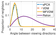
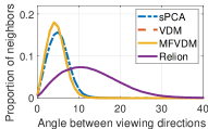
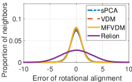
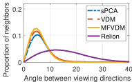
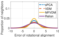
Nearest Neighbor Search: We evaluate nearest neighbor search by inspecting the distribution of angles between the viewing directions of nearest neighbor pairs, defined as $\theta_{ij}=\arccos\langle v_{i},v_{j}\rangle.$ Accurate search means all $\theta_{ij}$s in the same group should concentrate to $0$ within a small spherical cap. Since the viewing direction of each projection image is known, we plot the histograms of $\theta_{ij}$ for nearest neighbor lists identified by different appoaches. Fig. 6 shows, at high SNR, MFVDM and VDM have similar results. When $\text{SNR}=0.01$, MFVDM identifies more nearest neighbors that concentrate in the small spherical cap than other methods. This indicates that MFVDM is more robust to noise.

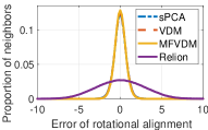
Rotational Alignment: We evaluate alignment by computing $\alpha_{ij}-\hat{\alpha}_{ij}$ for all pairs of nearest neighbors $(i,j)$, where $\alpha_{ij}$ is ground truth and $\hat{\alpha}_{ij}$ is the estimate. Fig. 6 shows the histograms of errors for all nearest neighbor pairs. Note that at $\text{SNR}=0.01$, MFVDM achieves more accurate estimation of in-plane rotational alignment than other methods, which indicates, again, MFVDM is more robust to noise.

Nearest neighbor search

(a)

Rotational alignment

(b)

SNR = 0.05

(c)

(d)

(e)

SNR = 0.02

(f)

(g)

(h)

SNR = 0.01

(i)

(j)

(k)

Figure 6: Histograms of Left: angles between viewing directions of nearest neighbors identified by different approaches, Right: rotational alignment errors by different approaches. The horizontal axes are in degrees. Rows show different noise levels $\text{SNR}=0.05,0.02,0.01$. Lines of VDM and MFVDM overlap in the top two rows.

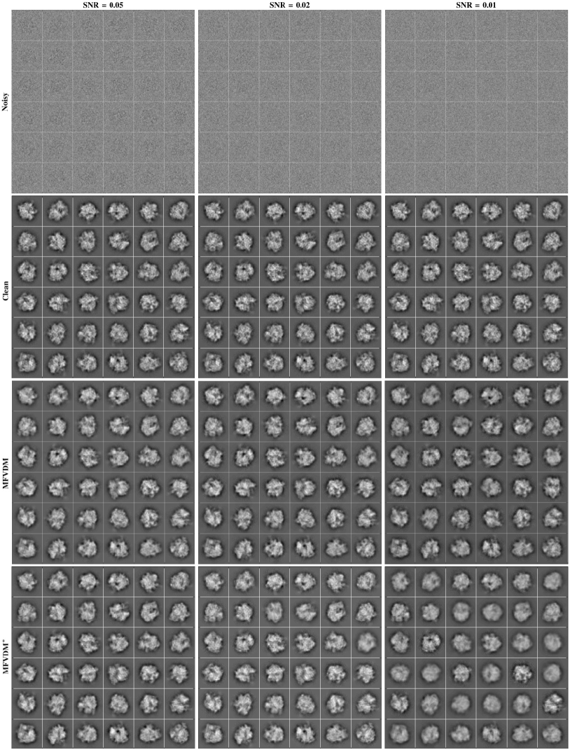
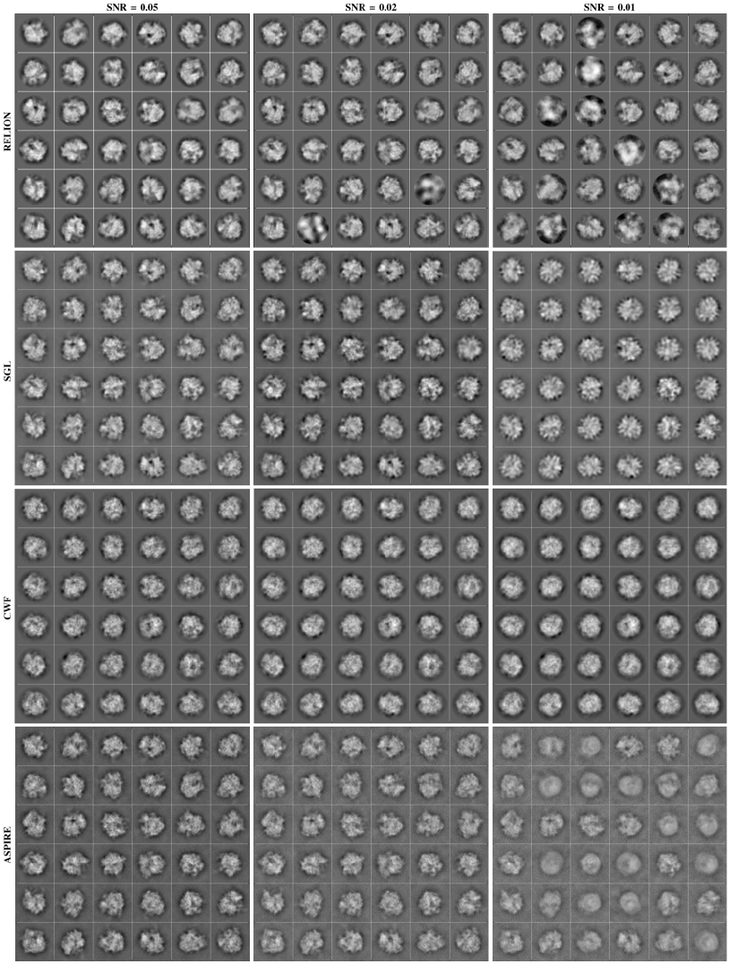
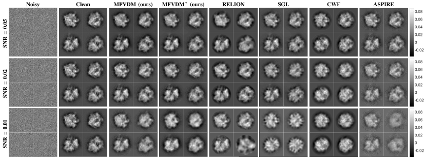
Denoising: Fig. 5 presents the denoising of CTF-affected image samples at various SNR levels. To emphasize the significance of a denoised graph by MFVDM (see Fig. 3), we use sPCA to build the noisy graph then denoising, which is denoted as MFVDM^∗. It can be seen that all methods preform well at high $\text{SNR}=0.05$. While at low SNR cases, MFVDM and RELION outperform SGL, CWF and ASPIRE, whose results are blurry and have lost detailed information. In addition, MFVDM outperforms MFVDM^∗, especially for $\text{SNR}=0.01$, this indicates the effects of MFVDM neighbor search and alignment. In Appendix we show more denoised results.

Figure 7: More sample images for denoising simulated projections from 70S ribosome, by MFVDM and RELION, at noise levels $\text{SNR}=0.05,0.02,0.01$.

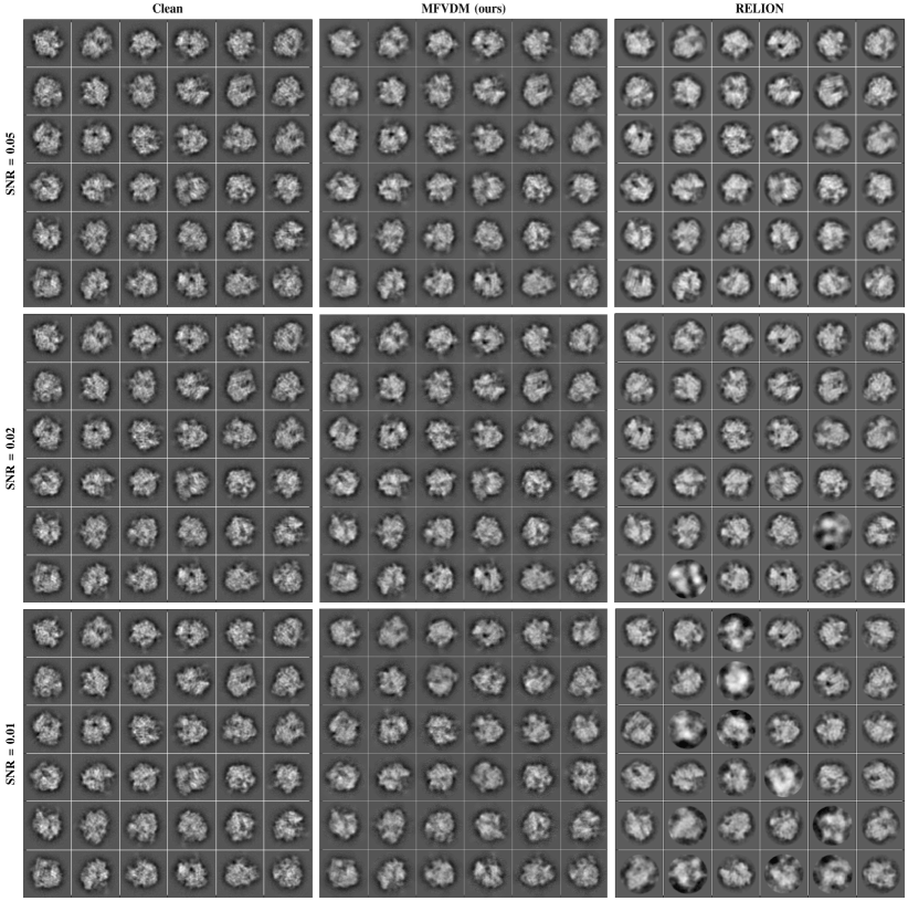
In Fig. 7 we present more denoising samples to compare the results from MFVDM and RELION, at $\text{SNR}=0.05,0.02,0.01$. It shows at high SNR, e,g, $\text{SNR}=0.05$, both methods achieve a good performance. While at lower SNR cases as $0.02$ or $0.01$, RELION could fail to denoise on some images, which are shown in chaos. Also a few images have been classified incorrectly. However, MFVDM still almost work. Again, this show the robustness of MFVDM.

TABLE I: Average MSE, PSNR and SSIM of denoised images on 70S ribosome. The reference are clean projection images without CTFs (see Fig. 2(a)).

SNR		MFVDM	MFVDM∗	SGL	CWF	ASPIRE
0.05	MSE	0.0177	0.0186	0.0193	0.0313	0.0376
	PSNR	47.7	47.3	47.2	45.2	44.3
	SSIM	0.966	0.965	0.963	0.943	0.950
0.02	MSE	0.0223	0.0267	0.0280	0.0487	0.0972
	PSNR	46.7	46.0	45.6	43.2	40.2
	SSIM	0.959	0.953	0.948	0.920	0.885
0.01	MSE	0.0383	0.0429	0.0527	0.0637	0.273
	PSNR	44.6	43.3	43.1	42.0	35.6
	SSIM	0.932	0.914	0.910	0.902	0.715

MSE, SSIM and PSNR: In Tab. I we present the average of mean squared error (MSE), peak SNR (PSNR) and structural similarity index (SSIM) on the denoised images. Notebly MFVDM outperforms other approaches with the smallest MSE and largest PSNR and SSIM, at all SNR levels. For RELION, since its denoising result includes unknown inplane shifts, we are unable to fairly evaluate such measurements on RELION.

Figure 8: 3D reconstructions of 70S ribosome using 1000 denoised images as shown in Fig. 5 at $\text{SNR}=0.01$.

Runtime: Tab. II compares the runtime of different approaches. We take $n=10^{4}$ noisy images with $\text{SNR}=0.01$ as input, and output all denoised ones. All methods use the same amount of computational resource (12 cores CPU). The MFVDM denosing, by building a nearest neighbor graph and filtering it, runs much faster than RELION which is an iterative procedure. Even though with GPU implementation, RELION still takes more time. The runtime of SGL and ASPIRE are similar to MFVDM due to their similar procedures. This demonstrates that MFVDM is more efficient compared to other approches.

TABLE II: The runtime (in minutes) of different methods on 70s ribosome, at $\text{SNR}=0.01$. RELION^∗ represents RELION with GPU acceleration.

MFVDM	RELION	RELION∗	SGL	CWF	ASPIRE
12	465	117	12	11	15

TABLE III: The volume resolutions (lower is better) for 70S ribosome

MFVDM	RELION	CWF	SGL	ASPIRE
14.8Å	25.4Å	44.4Å	39.5Å	17.7Å

Figure 9: Image samples of top: TRPV1; Bottom: HIV-1 Nef datasets. From left to right: raw images, closest projection: the clean projection images from the reference map that have the highest correlation with the noisy images estimated by RELION. the denoised results by MFVDM, RELION, CWF, SGL and ASPIRE.

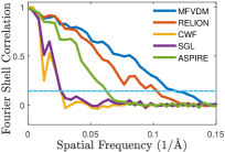
3D Ab Initio Model: The 3D ab initio modeling benefits from the improved denoising of 2D projection images. In Fig. 8, for each denoising method, we show the 3D reconstruction of 70S ribosome from 1000 denoised projection images (original $\text{SNR}=0.01$) using common-lines based algorithm [33]. The corresponding noisy images are the same for each method. It shows that only MFVDM achieves a comparatively accurate reconstruction and the results from other methods are noisy or lose significant sub-structures. In addition to visual inspection, we use the Fourier shell correlation (FSC) [5] between the reconstruction and the original volume to quantify the resolution, which is determined by the 0.143 cutoff of FSC (see Tab. III).

IV-B Experimental Datasets

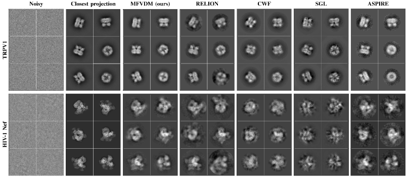
We test the performance of MFVDM on two public experimental datasets available in the Electron Microscope Pilot Image Archive (EMPIAR) [15]: (1) TRPV1 ion channel[13] (for brevity, TRPV1), (2) HIV-1 Nef[17]. Noisy samples are shown in the first column of Fig. 9. For each dataset we take $n=10^{4}$ images as input to perform each approach.

Colored Noise Whitening: Consider the experimental cryo-EM images are typically corrupted by colored noise, we need to first prewhiten the raw images: We estimate the power spectrum of noise based on the corner pixel values, since particles are contained in the middle of the images. Then we whiten each image using the estimated noise power spectrum and perform CTF correction via phase flipping. We perform nearest neighbor search, alignment, and denoising on the pre-processed images. After denoising, we recolor the denoised images by multiplying the estimated noise power spectrum in the Fourier domain and perform CTF correction based on (13).

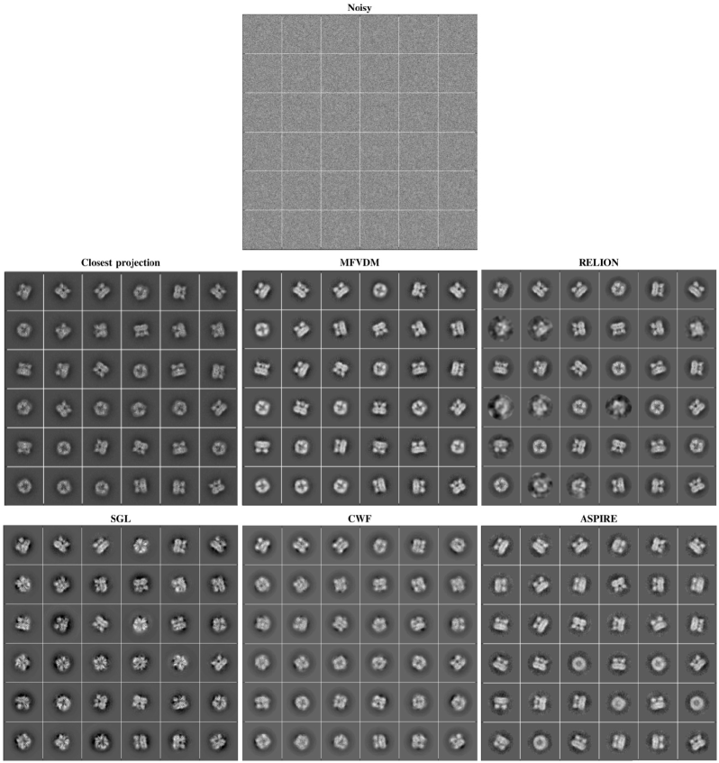
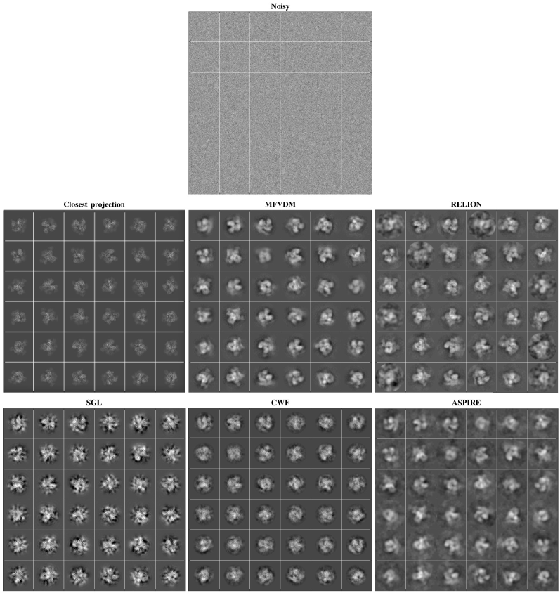
Denoising: The sample denoised images are displayed in Fig. 9. Here we generated the clean template images from the reference map and estimated the most similar template for each raw image. We used the 3D auto refine tool in RELION 2.1 to carry out the template matching (notice the closest projection may not be the truth beneath the raw image due to the high level of noise). Visually, MFVDM denoised images are cleaner than the results of other methods. Due to the lack of ground truths, i.e., particle orientations and clean images, we cannot compare the classification and alignment results as before, and provide the MSEs, SSIMs and PSNRs for the denoised images. To quantitatively evaluate the methods for 2D image analysis, we evaluate the 3D ab initio models constructed from those denoised images. In Appendix we show more denoised results.

Runtime: In Tab. IV we report the runtime of different approaches, for denoising $n=10^{4}$ images. Similar to the synthetic example, MFVDM denoising is the most efficient pipeline compared with other approaches.

TABLE IV: The runtime (in minutes) of different methods on TRPV1 and HIV-1 Nef datasets. RELION^∗ represents RELION with GPU acceleration.

Dataset	MFVDM	RELION	RELION∗	CWF	SGL	ASPIRE
TRPV1	43	366	284	82	51	63
HIV-1 Nef	32	308	127	71	36	49

TRPV1
HIV-1 Nef

Figure 10: 3D ab initio models of top: TRPV1; Bottom: HIV-1 Nef, with denoised images from MFVDM, RELION 2D class averaging, CWF, SGL, and ASPIRE 2D class averaging. Three views of the volumes are shown in columns. ’Ref.’ represents the reference volume, ‘Ref. Low Res.’ represents the Gaussian filtered reference volume.

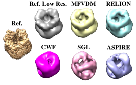
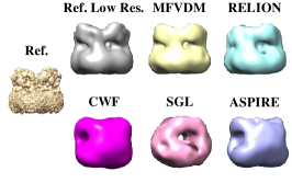
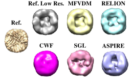
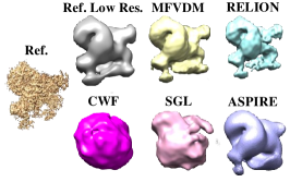
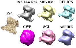
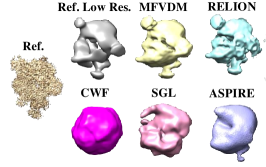
3D Ab Initio Model: In Fig. 10, we show the 3D ab initio models generated from 1000 denoised images with identical underlying noisy images. The TRPV1 volumes are generated by RELION 3D Initial Model with 50 iterations. The HIV-1 Nef volumes are generated by common-lines algorithm [33]. Fig. 10 shows that MFVDM and RELION are able to achieve good initial models that are similar to the Gaussian filtered reference volumes. Other methods lose significant sub-sructure. In addition, we compute the Fourier shell correlation (FSC) in Fig. 11. It shows that the reconstruction based on the MFVDM denoised images achieves the highest correlations and resolutions (see Tab. V) for both datasets. Our new pipeline outperforms the state-of-the-art methods and is able to efficiently produce accurate initial models for cryo-EM.

(a)

(b)

Figure 11: Fourier shell correlation (FSC) between the reconstruction and the Reference volume (high resolution). Blue dashed line is the 0.143 cut-off criterion. Left: TRPV1, Right: HIV-1 Nef.

TABLE V: The volume resolutions (lower is better) for TRPV1 and HIV-1 Nef.

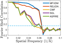
Dataset	MFVDM	RELION	CWF	SGL	ASPIRE
TRPV1	15.88Å	15.88Å	16.93Å	19.54Å	21.16Å
HIV-1 Nef	8.69Å	9.78Å	39.12Å	39.12Å	16.76Å

V Conclusion

Cryo-EM imaging will benefit from the cross fertilization of ideas with the computer vision community. Here, we proposed a new framework for cryo-EM image restoration by defining a new metric based on MFVDM to improve the rotationally invariant nearest neighbor search among a large number of extremely noisy images. This new metric takes into account of the consistency of the irreducible representations of the alignments along connected paths. The eigenvectors of the MFVDM matrices contain alignment information for images of similar views and are therefore used for optimal alignment estimation. The denoised graph structure allows the computation of robust global basis on the data manifold. The resulting graph filtering schemes are able to efficiently denoise the Fourier-Bessel expansion coefficients of the images and perform CTF correction. Through the simulated and experimental datasets, we demonstrated our proposed methods outperform the state-of-the-art 2D class averaging and image restoration algorithms.

-A More Experimental Results

In this section, we provide more experimental results on the simulated dataset (70S ribosome) and the experimental datasets (TRPV1 and HIV-1 Nef). The parameter setting is the same as the main paper.

Simulated Dataset: In Fig. 12 and Fig. 13 we show more denoised images of 70S ribosome by MFVDM, MFVDM^∗, RELION 2D class averaging, SGL, CWF, and ASPIRE 2D class averaging at SNR $=0.05,0.02,0.01$. All methods preform well at high SNR ($\text{SNR}=0.05$). As the noise level increases, MFVDM outperforms other methods. Some class averages generated from RELION does not have any structural information and a few images are classified incorrectly. SGL and CWF are able to denoise and preserve the main structure, but some detailed information has been lost. ASPIRE appears noisier due to the fact that it only averages $s$-nearest neighbors directly. It shows that compared with the existing methods, MFVDM is more robust to noise. In addition, the performance of MFVDM^∗ (without Alg. 1 in the main paper) is worse than MFVDM, especially at $\text{SNR}=0.01$, this indicates the importance of MFVDM nearest neighbor search and alignment.

Experimental Datasets: In Figs. 14 and 15 we show more denoising results for two experimental datasets: TRPV1 and HIV-1 Nef, by the following approaches: MFVDM, RELION 2D class averaging, SGL, CWF and ASPIRE 2D averaging. We generated the clean template images from the reference map and estimated the most similar template for each raw image. We used the 3D auto refine tool in RELION 2.1 to carry out the template matching (notice the closest projection may not be the truth beneath the raw image due to the high level of noise). The Figs. 14 and 15 show that our proposed method (MFVDM) is able to recover all views. RELION is good at recovering a few views, however, some class-means have very poor quality. The MFVDM and RELION 2D class averaing outperform CWF, SGL and ASPIRE on these real datasets.

For the real image data, we cannot use the estimated closest projections to directly evaluate 2D image denoising in terms of MSE, SSIM and PSNR, because (1) the real single particle images are not perfectly centered, and (2) the estimated closest projections might be inaccurate. Therefore, the quantitative evaluation for real data is through the comparisons of the resolution of the reconstructed volume and the Fourier shell correlations shown in the main paper.

Figure 12: Image samples of simulated 70S ribosome dataset. From top to bottom: noisy projection images, clean projection images and denoised results by MFVDM, MFVDM^∗. Columns show different noise levels $\text{SNR}=0.05,0.02,0.01$.

Figure 13: Image samples of simulated 70S ribosome dataset. From top to bottom: denoised results by RELION, SGL, CWF and ASPIRE. Columns show different noise levels $\text{SNR}=0.05,0.02,0.01$.

Figure 14: Image samples of TRPV1 dataset. Noisy: raw projection images. Closest projection: the clean projection images from the reference map that have the highest correlation with the noisy images estimated by RELION. MFVDM, RELION, SGL, CWF, ASPIRE: the corresponding denoised images.

Figure 15: Image samples of HIV-1 Nef dataset. Noisy: raw projection images. Closest projection: the clean projection images from the reference map that have the highest correlation with the noisy images estimated by RELION. MFVDM, RELION, SGL, CWF, ASPIRE: the corresponding denoised images.

References

- [1] T. Bhamre, T. Zhang, and A. Singer. Denoising and covariance estimation of single particle cryo-em images. Journal of structural biology, 195(1):72–81, 2016.
- [2] A. Buades, B. Coll, and J.-M. Morel. A non-local algorithm for image denoising. In Computer Vision and Pattern Recognition, 2005. CVPR 2005. IEEE Computer Society Conference on, volume 2, pages 60–65. IEEE, 2005.
- [3] S. H. Chan. Performance analysis of plug-and-play admm: A graph signal processing perspective. arXiv preprint arXiv:1809.00020, 2018.
- [4] J. De la Rosa-Trevín, J. Otón, R. Marabini, A. Zaldivar, J. Vargas, J. Carazo, and C. Sorzano. Xmipp 3.0: an improved software suite for image processing in electron microscopy. Journal of structural biology, 184(2):321–328, 2013.
- [5] J. Frank. Three-dimensional electron microscopy of macromolecular assemblies: visualization of biological molecules in their native state. Oxford University Press, 2006.
- [6] D. Giannakis, P. Schwander, and A. Ourmazd. The symmetries of image formation by scattering. i. theoretical framework. Optics express, 20(12):12799–12826, 2012.
- [7] G. Gilboa, N. Sochen, and Y. Y. Zeevi. Forward-and-backward diffusion processes for adaptive image enhancement and denoising. IEEE transactions on image processing, 11(7):689–703, 2002.
- [8] A. Heimowitz, J. Andén, and A. Singer. Apple picker: Automatic particle picking, a low-effort cryo-em framework. Journal of structural biology, 204(2):215–227, 2018.
- [9] Z. Kam. The reconstruction of structure from electron micrographs of randomly oriented particles. Journal of Theoretical Biology, 82:15–39, 1980.
- [10] B. Landa and Y. Shkolnisky. Steerable principal components for space-frequency localized images. SIAM journal on imaging sciences, 10(2):508–534, 2017.
- [11] B. Landa and Y. Shkolnisky. The steerable graph laplacian and its application to filtering image data-sets. arXiv preprint arXiv:1802.01894, 2018.
- [12] R. Langlois, J. Pallesen, J. T. Ash, D. N. Ho, J. L. Rubinstein, and J. Frank. Automated particle picking for low-contrast macromolecules in cryo-electron microscopy. Journal of structural biology, 186(1):1–7, 2014.
- [13] M. Liao, E. Cao, D. Julius, and Y. Cheng. Structure of the TRPV1 ion channel determined by electron cryo-microscopy. Nature, 504(7478):107, 2013.
- [14] C.-Y. Lin and H.-T. Wu. Embeddings of Riemannian manifolds with finite eigenvector fields of connection laplacian. arXiv preprint arXiv:1604.05707, 2016.
- [15] A. Ludin, P. K. Korir, J. Salavert-Torres, G. J. Kleywegt, and A. Patwardhan. EMPIAR: A public archive for raw electron microscopy image data. Nature Methods, 13(387–388):387–388, 2016.
- [16] D. Lyumkis, A. F. Brilot, D. L. Theobald, and N. Grigorieff. Likelihood-based classification of cryo-EM images using FREALIGN. Journal of structural biology, 183(3):377–388, 2013.
- [17] K. L. Morris, C. Z. Buffalo, C. M. Sturzel, E. Heusinger, F. Kirchhoff, X. Ren, and J. H. Hurley. HIV-1 Nefs are cargo-sensitive AP-1 trimerization switches in tetherin and MHC-I downregulation. bioRxiv, page 276733, 2018.
- [18] S. Osher, Z. Shi, and W. Zhu. Low dimensional manifold model for image processing. SIAM Journal on Imaging Sciences, 10(4):1669–1690, 2017.
- [19] A. Pascual-Montano, L. Donate, M. Valle, M. Barcena, R. Pascual-Marqui, and J. Carazo. A novel neural network technique for analysis and classification of em single-particle images. Journal of structural biology, 133(2-3):233–245, 2001.
- [20] P. A. Penczek. Image restoration in cryo-electron microscopy. In Methods in enzymology, volume 482, pages 35–72. Elsevier, 2010.
- [21] S. H. Scheres. Maximum-likelihood methods in cryo-EM. part II: Application to experimental data. Methods in enzymology, 482:295, 2010.
- [22] S. H. Scheres. Relion: Implementation of a bayesian approach to cryo-EM structure determination. Journal of Structural Biology, 180:519–530, 2012.
- [23] S. H. Scheres, R. Núñez-Ramírez, Y. Gómez-Llorente, C. San Martín, P. P. Eggermont, and J. M. Carazo. Modeling experimental image formation for likelihood-based classification of electron microscopy data. Structure, 15(10):1167–1177, 2007.
- [24] S. H. Scheres, M. Valle, R. Nuñez, C. O. Sorzano, R. Marabini, G. T. Herman, and J.-M. Carazo. Maximum-likelihood multi-reference refinement for electron microscopy images. Journal of molecular biology, 348(1):139–149, 2005.
- [25] P. Schwander, D. Giannakis, C. H. Yoon, and A. Ourmazd. The symmetries of image formation by scattering. ii. applications. Optics express, 20(12):12827–12849, 2012.
- [26] F. Sigworth. A maximum-likelihood approach to single-particle image refinement. Journal of structural biology, 122(3):328–339, 1998.
- [27] F. J. Sigworth. Principles of cryo-EM single-particle image processing. Microscopy, 65(1):57–67, 2016.
- [28] A. Singer, Y. Shkolnisky, and B. Nadler. Diffusion interpretation of nonlocal neighborhood filters for signal denoising. SIAM Journal on Imaging Sciences, 2(1):118–139, 2009.
- [29] A. Singer and H.-T. Wu. Vector diffusion maps and the connection laplacian. Communications on pure and applied mathematics, 65(8):1067–1144, 2012.
- [30] A. Singer, Z. Zhao, Y. Shkolnisky, and R. Hadani. Viewing angle classification of cryo-electron microscopy images using eigenvectors. SIAM Journal on Imaging Sciences, 4(2):723–759, 2011.
- [31] G. Tang, L. Peng, P. R. Baldwin, D. S. Mann, W. Jiang, I. Rees, and S. J. Ludtke. Eman2: an extensible image processing suite for electron microscopy. Journal of structural biology, 157(1):38–46, 2007.
- [32] C. Tomasi and R. Manduchi. Bilateral filtering for gray and color images. In Computer Vision, 1998. Sixth International Conference on, pages 839–846. IEEE, 1998.
- [33] L. Wang and A. Singer. Exact and stable recovery of rotations for robust synchronization. Information and Inference: A Journal of the IMA, 2(2):145–193, 2013.
- [34] L. Wang, A. Singer, and Z. Wen. Orientation determination of cryo-EM images using least unsquared deviations. SIAM journal on imaging sciences, 6(4):2450–2483, 2013.
- [35] D. J. Watts and S. H. Strogatz. Collective dynamics of ‘small-world’networks. nature, 393(6684):440, 1998.
- [36] J. Yang, J. Wright, T. S. Huang, and Y. Ma. Image super-resolution via sparse representation. IEEE transactions on image processing, 19(11):2861–2873, 2010.
- [37] R. Yin, T. Gao, Y. M. Lu, and I. Daubechies. A tale of two bases: Local-nonlocal regularization on image patches with convolution framelets. SIAM Journal on Imaging Sciences, 10(2):711–750, 2017.
- [38] Z. Zhao, Y. Shkolnisky, and A. Singer. Fast steerable principal component analysis. IEEE transactions on computational imaging, 2(1):1–12, 2016.
- [39] Z. Zhao and A. Singer. Fourier–bessel rotational invariant eigenimages. JOSA A, 30(5):871–877, 2013.
- [40] Z. Zhao and A. Singer. Rotationally invariant image representation for viewing direction classification in cryo-em. Journal of structural biology, 186(1):153–166, 2014.