Van der Pol - Duffing oscillator: global view of metamorphoses of the amplitude profiles

Abstract

Dynamics of the Duffing–Van der Pol driven oscillator is investigated. Periodic steady-state solutions of the corresponding equation are computed within the Krylov-Bogoliubov-Mitropolsky approach to yield dependence of amplitude $A$ on forcing frequency $\Omega$ as an implicit function, $F\left(A,\Omega\right)=0$, referred to as resonance curve or amplitude profile.

In singular points of the amplitude curve the conditions $\frac{\partial F}{\partial A}=0$, $\frac{\partial F}{\partial\Omega}=0$ are fulfilled, i.e. in such points neither of the functions $A=f\left(\Omega\right)$, $\Omega=g\left(A\right)$, continuous with continuous first derivative, exists. Near such points metamorphoses of the dynamics can occur. In the present work the bifurcation set, i.e. the set in the parameter space, such that every point in this set corresponds to a singular point of the amplitude profile, is computed.

Several examples of singular points and the corresponding metamorphoses of dynamics are presented.

1 Introduction

In this paper we continue our study of the Duffing - van der Pol (DvdP) oscillator [1] which has been extensively investigated due to exhibiting interesting, complicated dynamics and to potential applications in physics, chemistry, biology, engineering, electronics, and many other fields, see [2, 3, 4, 5, 6, 7, 8, 9, 10, 11].

In [1] we studied metamorphoses of the amplitude profiles, obtained within the Krylov-Bogoliubov-Mitropolsky (KBM) approach, induced by changes of control parameters near singular points of these curves. In the present work we determine the bifurcation set – the space of parameters $C$, such that for every $C$ the amplitude curve $L\left(\Omega,\ A;\ C\right)=0$ has a singular point (this definition bears some similarity to the definition of the bifurcation set in the Catastrophe Theory [12]). Since qualitative changes of dynamics occur in neighbourhoods of singular points [13, 14, 15] we obtain in this way a global view of bifurcation parameters.

We consider the more general periodically forced Duffing - van der Pol oscillator with nonlinear damping which can be written as:

$$\dfrac{d^{2}x}{dt^{2}}-\left(b-cx^{2}\right)\dfrac{dx}{dt}+e\left(\frac{dx}{dt}\right)^{3}+ax+dx^{3}=f\cos\omega t.$$ (1)

There are three main cases of the Duffing potential $V\left(x\right)=\frac{1}{2}ax^{2}+\frac{1}{4}dx^{4}$: (i) single well $\left(a>0\text{,}\ d>0\right)$, (ii) double well $\left(a<0\text{, }d>0\right)$, and (iii) double hump $\left(a>0\text{,}\ d<0\right)$ . In the present paper we consider cases (i), ( iii) and it is thus assumed that $a,b,c,f,\omega>0$ while $d,e$ are arbitrary. For $e=0$ the DvdP model is recovered.

We compute periodic steady-state solutions of the DvdP equation within the Krylov-Bogoliubov-Mitropolsky (KBM) approach [16] to get dependence of amplitude on forcing frequency as an implicit function, referred to as resonance curve or amplitude profile. We investigate metamorphoses of the computed amplitude profiles induced by changes of control parameters near singular points of these curves since qualitative changes of dynamics occur in neighbourhoods of singular points, see [15] and references therein. The idea to use Implicit Function Theorem in this context was proposed in [17].

The paper is organized as follows. In the next Section the DvdP equation is written in nondimensional form and implicit equation for resonance curves $L\left(\Omega,\ A\right)=0$ is derived via the KBM approach. In Section 3 theory of algebraic curves is applied to compute the bifurcation set for the DvdP equation ($e=0$) which yields a global view of bifurcations. In Section 4 examples of metamorphoses of dynamics occurring in neighbourhoods of singular points are presented. We summarize our results in the last Section.

2 Nonlinear resonances via KBM method

A very exact generalized harmonic balance method was developed by Luo [18]. We apply to Eq. (1) less exact but sufficient in case of steady-states the Krylov-Bogoliubov-Mitropolsky perturbation approach [16]. Substituting into (1):

$$x=\sqrt{\tfrac{b}{c}}z,\ t=\tfrac{1}{\sqrt{a}}\tau,\ \omega=\sqrt{a}\Omega,$$ (2)

we get the DvdP equation in nondimensional form:

$$\begin{array}[]{c}\dfrac{d^{2}z}{d\tau^{2}}-\mu\left(1-z^{2}\right)\dfrac{dz}{d\tau}+\nu\left(\frac{dz}{d\tau}\right)^{3}+z+\lambda z^{3}=G\cos\left(\Omega\tau\right),\\ \mu,\ G,\ \Omega>0,\quad\lambda,\ \nu\text{ -- arbitrary,}\end{array}$$ (3)

where $\mu=\frac{b}{\sqrt{a}}$, $\nu=\frac{\sqrt{a}be}{c}$, $\lambda=\frac{bd}{ac}$, $G=\frac{f}{a}\sqrt{\frac{c}{b}}$

The equation (3) is written in the following form:

$$\frac{d^{2}z}{d\tau^{2}}+\Omega^{2}z+\varepsilon\left(\sigma z+g\right)=0,$$ (4)

where

$$\left.\begin{array}[]{rl}g=&-\Theta_{0}^{2}z-\mu_{0}\dfrac{dz}{d\tau}+\mu_{0}z^{2}\dfrac{dz}{d\tau}+\nu_{0}\left(\frac{dz}{d\tau}\right)^{3}+\alpha_{0}z+\lambda_{0}z^{3}-G_{0}\cos\left(\Omega\tau\right)\\ \Theta_{0}^{2}=&\dfrac{\Theta^{2}}{\varepsilon},\ \mu_{0}=\dfrac{\mu}{\varepsilon},\ \nu_{0}=\dfrac{\nu}{\varepsilon},\ \alpha_{0}=\dfrac{1}{\varepsilon},\ \lambda_{0}=\dfrac{\lambda}{\varepsilon},\ G_{0}=\dfrac{G}{\varepsilon},\ \varepsilon\sigma=\Theta^{2}-\Omega^{2}\end{array}\right\}.$$ (5)

According to the KBM method we assume for small nonzero $\varepsilon$ that the solution for $1:1$ resonance can be written as:

$$z=A\left(\tau\right)\cos\left(\Omega\tau+\varphi\left(\tau\right)\right)+\varepsilon z_{1}\left(A,\varphi,\tau\right)+\ldots$$ (6)

with slowly varying amplitude and phase:

$$\dfrac{dA}{d\tau} = \varepsilon M_{1}\left(A,\varphi\right)+\ldots\ ,$$ (7)

$$\dfrac{d\varphi}{d\tau} = \varepsilon N_{1}\left(A,\varphi\right)+\ldots\ .$$ (8)

Computing now derivatives of $z$ from Eqs.(6), (7), (8) and substituting to Eqs.(4), (5), eliminating secular terms and demanding $M_{1}=0$, $N_{1}=0$ we obtain the following equations for the amplitude and phase of steady states:

$$A^{2}\Omega^{2}\left(\mu\left(1-\tfrac{1}{4}A^{2}\right)-\tfrac{3}{4}\nu A^{2}\Omega^{2}\right)^{2}+A^{2}\left(1+\tfrac{3}{4}\lambda A^{2}-\Omega^{2}\right)^{2}=G^{2}.$$ (9)

3 General properties of the amplitude profile $A\left(\Omega\right)$

3.1 Singular points

After introducing new variables, $\Omega^{2}=X$, $A^{2}=Y$, the equation ( 9) defining the amplitude profile reads $L\left(X,Y;\lambda,\mu,\nu,G\right)=0$ where:

$$L\left(X,Y\right)=XY\left(\mu\left(1-\tfrac{1}{4}Y\right)-\tfrac{3}{4}\nu YX\right)^{2}+Y\left(1+\tfrac{3}{4}\lambda Y-X\right)^{2}-G^{2}=0.$$ (10)

Singular points of $L\left(X,Y\right)$ are computed from equations [19]:

$$L = 0,$$ (11a)

$$\tfrac{\partial L}{\partial X} = 0,$$ (11b)

$$\tfrac{\partial L}{\partial Y} = 0.$$ (11c)

In [1] we have found several analytic solutions of Eqs. (11) for the DvdP equation, $$\nu=0$$.

3.2 Bifurcation set

It follows from general theory of implicit functions that in a singular point there are multiple solutions of equation (10). We shall use this property to compute parameters values for which singular points occur for the DvdP equation (i.e. for $\nu=0$).

Equation (11b) means that the function $X=f\left(Y\right)$ does not exist in the neighbourhood of a solution of Eqs. (11a), while due to Eq. (11c) also the function $Y=g\left(X\right)$ does not exist (more exactly, there are no continuous functions $f$, $g$ with continuous first derivatives $\frac{df}{dY}$, $\frac{dg}{dX}$).

On the other hand, to define a singular point we can use equations ( 11a), (11b) and an alternative of condition (11c) which excludes existence of the single-valued function $Y=g\left(X\right)$. We thus solve Eqs. (11a), (11b) obtaining equation for a function $Y=g\left(X\right)$ and then demand that there are multiple solutions for such $Y$ (alternatively, we could have solved Eqs. (11a), (11c)).

Solution of Eqs. (11a), (11b), with $L\left(X,Y\right)$ given by Eq. (10) (note that we have set $\nu=0$) can be written as a quintic equation for $Y$:

$$\left.\begin{array}[]{l}F\left(Y\right)=a_{5}Y^{5}+a_{4}Y^{4}+a_{3}Y^{3}+a_{2}Y^{2}+a_{1}Y+a_{0}=0,\vskip 6.0pt plus 2.0pt minus 2.0pt\\ a_{5}=\mu^{4},\ a_{4}=-16\mu^{2}\left(\mu^{2}+3\lambda\right),\ a_{3}=32\mu^{2}\left(3\mu^{2}+12\lambda-2\right),\vskip 3.0pt plus 1.0pt minus 1.0pt\\ a_{2}=-256\mu^{2}\left(\mu^{2}+3\lambda-2\right),\ a_{1}=256\mu^{2}\left(\mu^{2}-4\right),\ a_{0}=1024G^{2},\end{array}\right\}$$ (12a)

with $$X$$ given by:

$$X=-\tfrac{1}{32}\mu^{2}Y^{2}+\left(\tfrac{1}{4}\mu^{2}+\tfrac{3}{4}\lambda\right)Y-\tfrac{1}{2}\mu^{2}+1,$$ (12b)

and we assume that $$\mu\neq 0$$.

Equation (12b) is identical with Eq. (16) in ([1]) which for $G\neq 0$ determines the general solution of Eqs. (11) (note that the text after Eq. (14) in ([1]) should read: equation for $\mu$: $B_{6}\mu^{6}+B_{4}\mu^{4}+B_{2}\mu^{2}+B_{0}=0$).

Necessary condition for a polynomial to have multiple roots is that its discriminant vanishes [20]. Discriminant $\Delta$ can be computed as a resultant of a polynomial $F\left(Y\right)$ and its derivative $F^{\prime}$, with a suitable normalizing factor. Resultant of a quintic polynomial $F\left(Y\right)=a_{5}Y^{5}+a_{4}Y^{4}+a_{3}Y^{3}+a_{2}Y^{2}+a_{1}Y+a_{0}$ and its derivative $F^{\prime}$ is given by determinant of the Sylvester matrix $S$, $\Delta=a_{5}^{-1}\det\left(S\right)$ where [20]:

$$S=\left(\begin{array}[]{ccccccccc}a_{0}&a_{1}&a_{2}&a_{3}&a_{4}&a_{5}&0&0&0\\ 0&a_{0}&a_{1}&a_{2}&a_{3}&a_{4}&a_{5}&0&0\\ 0&0&a_{0}&a_{1}&a_{2}&a_{3}&a_{4}&a_{5}&0\\ 0&0&0&a_{0}&a_{1}&a_{2}&a_{3}&a_{4}&a_{5}\\ a_{1}&2a_{2}&3a_{3}&4a_{4}&5a_{5}&0&0&0&0\\ 0&a_{1}&2a_{2}&3a_{3}&4a_{4}&5a_{5}&0&0&0\\ 0&0&a_{1}&2a_{2}&3a_{3}&4a_{4}&5a_{5}&0&0\\ 0&0&0&a_{1}&2a_{2}&3a_{3}&4a_{4}&5a_{5}&0\\ 0&0&0&0&a_{1}&2a_{2}&3a_{3}&4a_{4}&5a_{5}\end{array}\right).$$ (13)

For explicit formula for a discriminant of the quintic polynomial see Eq. (1.36) in Chapter 12 in [20].

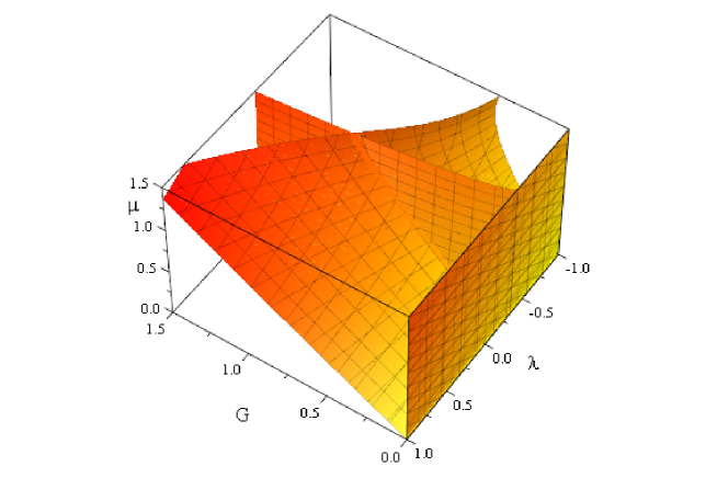
Figure 1: The bifurcation set: $D\left(G,\lambda,\mu\right)=0$, $G=0$, see Eq. (14)

The discriminant $\Delta$ for polynomial $F(Y)$ in Eq. (12a) is:

$$\left.\begin{array}[]{l}\Delta=2^{40}\mu^{10}G^{2}\,D\left(G,\lambda,\mu\right),\quad\left(\mu\neq 0\right)\\ D\left(G,\lambda,\mu\right)=A_{10}\mu^{10}+A_{8}\mu^{8}+A_{6}\mu^{4}+A_{4}\mu^{4}+A_{2}\mu^{2}+A_{0},\end{array}\right\}$$ (14)

with coefficients $A_{i}$ given in the appendix.

Therefore, condition $\Delta=0$ yields the bifurcation set:

$$D\left(G,\lambda,\mu\right)=0,\text{ or }G=0,$$ (15)

the manifold of singular points in the parameter space $\left(G,\lambda,\mu\right)$, see Fig. 1 where a fragment of the surface $D\left(G,\lambda,\mu\right)=0$ as well as the plane $G=0$ are plotted:

The surface $D\left(G,\lambda,\mu\right)=0$ may be considered as consisting of two intersecting surfaces. There are thus three families of singular points: lying on one surface, lying on another surface, and the third family consists of points lying on a curve – the intersection of these two surfaces.

3.3 Double singular points

Double singular points – points belonging to the self-intersection of the surface $D\left(G,\lambda,\mu\right)=0$ – can be computed numerically. It follows from Fig. 1 that for $\mu=\mu_{0}>0$ there is a singular point on the curve obtained by intersecting the surface $D=0$ by the plane $\mu=\mu_{0}$, i.e. on the curve $D\left(G,\lambda,\mu_{0}\right)=0$. Therefore, the intersection curve can be computed in the following way. If we set $\mu=\mu_{0}$, then $\lambda$, $G$ can be computed from equations:

$$\frac{\partial D\left(G,\lambda,\mu_{0}\right)}{\partial G} = 0,$$ (16a)

$$\frac{\partial D\left(G,\lambda,\mu_{0}\right)}{\partial\lambda} = 0,$$ (16b)

which define a singular point on the curve $$D\left(G,\lambda,\mu_{0}\right)=0 G_{0},\lambda_{0},\mu_{0} D\left(G_{0},\lambda_{0},\mu_{0}\right)=0 D=0 \mu_{0}>0$$. Since there are several solutions of equations (16), mostly complex, we have to choose the right solution , i.e. such that fulfills , i.e. lies on the surface . It follows from Fig. 1 that for such solution exists.

There are also other double singular points – belonging to intersection of surfaces $\Delta=0$ and $G=0$. Solving equations:

$$\Delta = 0,$$ (17a)

$$G = 0,$$ (17b)

we obtain a very simple condition:

$$4096\mu^{4}\left(\mu-2\right)^{2}\left(\mu+2\right)^{2}\left(3\lambda+1\right)^{3}\left(9\lambda^{2}+\mu^{2}+3\lambda\mu^{2}\right)=0.$$ (18)

We shall investigate below the solution $\mu=2$, $\lambda$ – arbitrary. More exactly, we shall consider the case $\mu=2$, $\lambda\geq-\left|a\right|$ with small values of $\left|a\right|$ since for more negative values of $\lambda$ the system is unstable – trajectories escape to infinity.

4 Computational results

A global picture of singular points, shown in the bifurcation set, Fig. 1, can be used to predict metamorphoses of dynamics. In our previous work [1] we have described metamorphoses occuring near singular poitns belonging to the plane $G=0$. It is now obvious, that all points of the plane $G=0$ in the parameter space $\left(G\text{, }\lambda\text{, }\mu\right)$ are singular – they are isolated points of the amplitude profile, cf. Eq. (15). Such metamorphosis is described in Section 4.1 in [1] for $\lambda=1$, $\mu=0.5$.and $G\geq 0$.

In this work we study metamorphoses occuring near double singular points: belonging to self-intersection of the surface $D\left(G,\lambda,\mu\right)=0$ and belonging to intersection of the surface $D\left(G,\lambda,\mu\right)=0$ and the plane $G=0$, see Fig. 1.

We first compute a point lying on the self-intersection curve in Fig. 1. For $\mu_{0}=3$ we get from Eqs. (16) solution $\lambda_{0}=-0.118\,321$, $G_{0}=1.\,214\,842$ which fulfills $\Delta\left(G_{0},\lambda_{0},\mu_{0}\right)=0$. Now we plot the corresponding amplitude profile, i.e. the implicit function $A\left(\Omega\right)$ given by Eq. (9) for parameters values $\lambda=\lambda_{0}$, $\mu=\mu_{0}$, $G<G_{0}$, $G=G_{0}$, $G>G_{0}$. The amplitude function $A\left(\Omega;G_{0},\lambda_{0},\mu_{0}\right)$ shown in Fig. 2 has two singular points – two self-intersections for $\Omega\simeq 0.12$ and $\Omega\simeq 0.28$, see Fig. 2. Green line corresponds to $G<G_{0}$, red line is the singular case, $G=G_{0}$, while blue line denotes the case $G>G_{0}$.

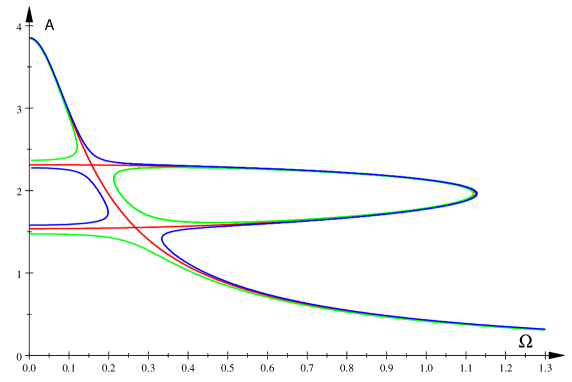
Figure 2: The amplitude profiles $A(\Omega)$, $\lambda=-0.118321$,$\mu=3$ and $G=1.19$ (green), $G_{0}=1.214842$ (red), and $G=1.23$ (blue).

Presence of these two singular points can be demonstrated by computing bifurcations diagrams.

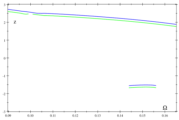
Figure 3: Bifurcation diagram. $G=1.2418<G_{0}$, $\mu=3$, $\lambda=-0.118321$ (green), $G=1.2419>G_{0}$. $\mu=3$, $\lambda=-0.118321$ (blue). Blue line shifted vertically by $0.12$.

In Fig. 3 the bifurcation diagram is shown for $G<G_{0}$, i.e. green line in Fig. 2. For $\Omega<0.12$ only the upper green branch is stable. Then, near $\Omega\simeq 0.12$ two upper branches disappear while the lowest branch is still unstable. Then, for $\Omega\simeq 0.2$ there are again three green branches in Fig. 2 – the upper branch is stable while the lowest branch is stable as well. In Fig. 3 we have $G>G_{0}$ corresponding to blue amplitude profile in Fig. 2. The upper branch is stable all through and of two lower branches the lowest is stable.

Induced dynamics near the second self-intersection is best demonstrated for $\mu=1$. For $\mu_{0}=1$ we get from Eqs. (16) solution $\lambda_{0}=-0.149\,954$, $G_{0}=0.662\,017$ which fulfills $\Delta\left(G_{0},\lambda_{0},\mu_{0}\right)=0$. Now we plot the corresponding amplitude profile, i.e. the implicit function $A\left(\Omega\right)$ given by Eq. (9) for parameters values $\lambda=\lambda_{0}$, $\mu=\mu_{0}$, $G<G_{0}$, $G=G_{0}$, $G>G_{0}$. The amplitude function $A\left(\Omega;G_{0},\lambda_{0},\mu_{0}\right)$ is shown in Fig. 4.

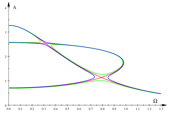
Figure 4: The amplitude profiles $A(\Omega)$, $\lambda=-0.118321$, $\mu=1$ and $G=0.65$ (green), $G=0.662017$ (red), and $G=0.67$ (blue).

Dynamics in the neighbourhood of the second self-intersection is shown in Fig. 5. It turns out that only lower branches are stable (for time running backwards). Therefore, the blue branch has a gap, while the green branch is continuous.

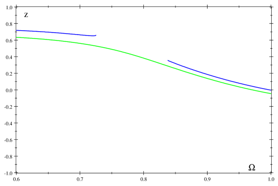
Figure 5: Bifurcation diagram. $\lambda=-0.118321$, $\mu=1$, $G=0.65$ (green), and $G=0.67$ (blue). Blue line shifted vertically by $0.05$.

Finally, we compute the amplitude profile for $G\geq 0$, $\mu=2$ and $\lambda=-0.1$. There are two singular points corresponding to $G=0$. The amplitude profiles are shown in Fig. 6 for $G=0.1$, $G=0.5$, $G=1$, $G=1.11$, $G=1.34$.

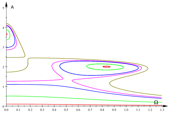
Figure 6: The amplitude profiles $A(\Omega)$, $\mu=2$, $\lambda=-0.1$, $G=0.1$ (red), $G=0.5$ (green), $G=1$ (blue), $G=1.11$ (magenta), $G=1.34$ (brown).

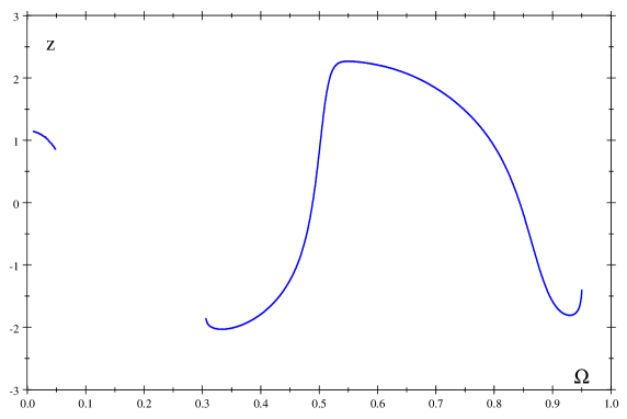
Figure 7: Bifurcation diagram, $\mu=2$, $\lambda=-0.1$, $G=1$ (cf. the blue line in Fig. 6).

In Fig. 7 the corresponding stable branches are shown for $G=1$.

5 Summary and discussion

In this work we have investigated dynamics of the periodically forced Duffing-van der Pol equation, continuing our study [1]. We were able to compute the bifurcation set – the set of all parameters, such that the amplitude profile has a singular point, see Eq. (15) and Fig. 1. We have thus obtained a global view of singular points computing all singular points in a novel way. Instead of solving the set of equations (11) we have solved Eqs. (11a), (11b) for $Y$, $X$ obtaining Eqs. (12a), (12b) and demanded that Eq. (12a) has multiple solutions. Note that Eq. (12b) and Eq. (16) from Ref. [1] are identical. This suggests that the bifurcation set contains all singular points since Eq. (16) determines the general solution of Eqs. (11) for $G\neq 0$. It seems that the method is general and can be applied to other dynamical systems.

It is interesting that there are double singular points, i.e. there are two singular points on the amplitude profile for some parameter values, see Figs. 2, 4, 6. In Section 4 the amplitude profiles and the corresponding bifurcation diagrams have been computed to show metamorphoses of dynamics near these singular points.

Appendix A Coefficients of the polynomial $D$, Eq. (14)

In this appendix coefficients of the polynomial (14) are listed below.

$$\left.\begin{array}[]{lll}\mathbf{A}_{\mathbf{10}}&\mathbf{=\vskip 6.0pt plus 2.0pt minus 2.0pt}&2^{8}\left(G+2+6\lambda\right)^{2}\left(G-2-6\lambda\right)^{2}\vskip 6.0pt plus 2.0pt minus 2.0pt\\ \mathbf{A}_{\mathbf{8}}&=&b_{5}\lambda^{5}+b_{4}\lambda^{4}+b_{3}\lambda^{3}+b_{2}\lambda^{2}+b_{1}\lambda+b_{0}\\ b_{5}&=&2^{12}3^{5}\\ b_{4}&=&-2^{12}3^{4}5\\ b_{3}&=&-2^{8}3^{3}\left(71G^{2}+2^{4}29\right)\\ b_{2}&=&-2^{8}3^{2}\left(3\times 19G^{2}+2^{4}47\right)\\ b_{1}&=&2^{6}3\left(-5G^{4}+2^{2}3^{2}7G^{2}-2^{11}\right)\\ b_{0}&=&2^{6}\left(-5^{2}G^{4}+2^{2}7^{2}G^{2}-2^{9}\right)\vskip 6.0pt plus 2.0pt minus 2.0pt\\ \mathbf{A}_{\mathbf{6}}&=&c_{5}\lambda^{5}+c_{4}\lambda^{4}+c_{3}\lambda^{3}+c_{2}\lambda^{2}+c_{1}\lambda+c_{0}\\ c_{5}&=&-2^{15}3^{5}\\ c_{4}&=&2^{15}3^{4}\left(G^{2}-1\right)\\ c_{3}&=&2^{11}3^{3}\left(157G^{2}+2^{4}5\right)\\ c_{2}&=&2^{6}3^{2}\left(-5\times 7\times 11G^{4}+2^{2}23\times 83G^{2}+2^{9}11\right)\\ c_{1}&=&2^{5}3\left(-5^{2}61G^{4}+2^{7}61G^{2}+2^{13}\right)\\ c_{0}&=&3125G^{6}-24\,000G^{4}+43\,008G^{2}+65\,536\vskip 6.0pt plus 2.0pt minus 2.0pt\\ \mathbf{A}_{\mathbf{4}}&=&d_{5}\lambda^{5}+d_{4}\lambda^{4}+d_{3}\lambda^{3}+d_{2}\lambda^{2}+d_{1}\lambda+d_{0}\\ d_{5}&=&2^{14}3^{5}\left(7G^{2}+2^{2}\right)\\ d_{4}&=&2^{13}3^{5}\left(19G^{2}+2^{3}\right)\\ d_{3}&=&2^{9}3^{4}\left(-3\times 5\times 11G^{4}+2^{3}3^{2}G^{2}+2^{7}\right)\\ d_{2}&=&2^{9}3^{2}\left(-5^{2}31G^{4}-2^{2}5\times 47G^{2}+2^{7}\right)\\ d_{1}&=&-2^{7}3^{3}G^{2}\left(5^{3}G^{2}+2^{5}11\right)\\ d_{0}&=&-2^{12}3^{3}G^{2}\vskip 6.0pt plus 2.0pt minus 2.0pt\\ \mathbf{A}_{\mathbf{2}}&=&e_{6}\lambda^{6}+e_{5}\lambda^{5}+e_{4}\lambda^{4}+e_{3}\lambda^{3}+e_{2}\lambda^{2}\\ e_{6}&=&2^{16}3^{6}G^{2}\\ e_{5}&=&2^{17}3^{5}G^{2}\\ e_{4}&=&-2^{15}3^{4}G^{2}\left(3\times 5G^{2}+7\right)\\ e_{3}&=&-2^{14}3^{3}G^{2}\left(5^{2}G^{2}+2\times 3^{2}\right)\\ e_{2}&=&-2^{12}3^{5}G^{2}\vskip 6.0pt plus 2.0pt minus 2.0pt\\ \mathbf{A}_{\mathbf{0}}&=&-2^{18}3^{5}G^{4}\lambda^{5}\end{array}\right\}$$ (19)

Appendix B Computational details

Nonlinear polynomial equations were solved numerically using the computational engine Maple from Scientific WorkPlace 5.5. All Figures were plotted with the computational engine MuPAD from Scientific WorkPlace 5.5. Curves shown in bifurcation diagrams in Figs. 3, 5, 7 were computed running DYNAMICS, program written by Helena E. Nusse and James A. Yorke.

References

• [1] J. Kyzioł and A. Okniński, The Duffing–Van der Pol Equation: Metamorphoses of Resonance Curves, Nonlinear Dynamics and Systems Theory, 15 (2015) 25-31.
• [2] W. Szemplińska-Stupnicka, J. Rudowski, The coexistence of periodic, almost-periodic and chaotic attractors in the van der Pol-Duffing oscillator, J. Sound Vibr. 199(2), 165-175 (1997).
• [3] A. Chudzik, P. Perlikowski, A. Stefański, T. Kapitaniak, Multistability and rare attractors in van der Pol-Duffing oscillator, Int. J. Bif. Chaos 21(7), 1907-1912 (2011).
• [4] S. Brezetskyi, D. Dudkowski, and T. Kapitaniak, Rare and hidden attractors in Van der Pol-Duffing oscillators, Eur. Phys. J. Special Topics 224, 1459-1467 (2015).
• [5] U. E. Vincent, B. R. Nana Nbendjo, A. A. Ajayi, A. N. Njah, P. V. E. McClintock, Hyperchaos and bifurcations in a driven Van der Pol–Duffing oscillator circuit, Int. J. Dynam. Control 3, 363–370 (2015).
• [6] V. Wiggers and P. C. Rech, On symmetric and asymmetric Van der Pol-Duffing oscillators, Eur. Phys. J. B 91, 144 (2018), 6 pages.
• [7] Q. Bi, Dynamical analysis of two coupled parametrically excited van der Pol oscillators, International J. Nonlinear Mech. 39 (2004) 33–54.
• [8] H. Chen, Q. Xu, Global bifurcations in externally excited autoparametric systems, International J. Nonlinear. Mech. 45 (2010) 766–792.
• [9] Yue Yu, Min Zhao, Zhengdi Zhang, Novel bursting patterns in a Van der pol-Duffing oscillator with slow varying external force, Mechanical Systems and Signal Processing 93, 164-174 (2017).
• [10] A.N. Njah, U.E. Vincent, Chaos synchronization between single and double wells Duffing–Van der Pol oscillators using active control, Chaos, Solitons and Fractals 37, 1356–1361 (2008).
• [11] A. C. J. Luo, A. B. Lakeh, Period-m motions and bifurcation trees in a periodically forced, van der Pol-Duffing oscillator, International Journal of Dynamics and Control 2.4 (2014): 474-493.
• [12] T. Poston, and I. Stewart, Catastrophe theory and its applications. Courier Corporation, Dover Publications, Inc., Mineola, New York, 2014.
• [13] J. Kyzioł, A. Okniński, Exact nonlinear fourth-order equation for two coupled oscillators: metamorphoses of resonance curves, Acta Phys. Polon. B44(1), 35-47 (2013).
• [14] J. Kyzioł, Metamorphoses of resonance curves for two coupled oscillators: The case of small non-linearities in the main mass frame, Int. J. Nonlinear Mech. 76 (2015) 164–168.
• [15] J. Kyzioł, A. Okniński, Metamorphoses of resonance curves in systems of coupled oscillators: The case of degenerate singular points, International Journal of Non-Linear Mechanics 95, 272–276 (2017).
• [16] A.H. Nayfeh, Introduction to Perturbation Techniques, John Wiley & Sons, 2011.
• [17] J. Awrejcewicz, Modified Poincaré method and implicit function theory, in: Nonlinear Dynamics: New Theoretical and Applied Results, J. Awrejcewicz (ed.), Akademie Verlag, Berlin, 1995, pp. 215-229.
• [18] A. C. J. Luo, Continuous dynamical systems, L & H Scientific Pub. and Higher Education Press Limited, 2012.
• [19] C. T. C. Wall, Singular Points of Plane Curves. New York, Cambridge University Press, 2004.
• [20] I.M. Gelfand, M.M. Kapranov, A.V. Zelevinsky, Discriminants, Resultants, and Multidimensional Determinants, Birkhäuser, Boston, MA, 1994.