Quantum partition of energy for a free Brownian particle:
Impact of dissipation

Abstract

We study the quantum counterpart of the theorem on energy equipartition for classical systems. We consider a free quantum Brownian particle modelled in terms of the Caldeira-Leggett framework: a system plus thermostat consisting of an infinite number of harmonic oscillators. By virtue of the theorem on the averaged kinetic energy $E_{k}$ of the quantum particle, it is expressed as $E_{k}=\langle\mathcal{E}_{k}\rangle$, where $\mathcal{E}_{k}$ is thermal kinetic energy of the thermostat per one degree of freedom and $\langle...\rangle$ denotes averaging over frequencies $\omega$ of thermostat oscillators which contribute to $E_{k}$ according to the probability distribution $\mathbb{P}(\omega)$. We explore the impact of various dissipation mechanisms, via the Drude, Gaussian, algebraic and Debye spectral density functions, on the characteristic features of $\mathbb{P}(\omega)$. The role of the system-thermostat coupling strength and the memory time on the most probable thermostat oscillator frequency as well as the kinetic energy $E_{k}$ of the Brownian particle is analysed.

I Introduction

Quantum physics shows that its world can exhibit behavior which is radically different than its classical counterpart. Wave-particle duality, entanglement of states, decoherence, Casimir force, quantum information - there are generic examples which in turn carry the potential for new applications in the near or further future. Yet, there still remain new properties, behavior and phenomena to be uncovered for this world. In this context, the quantum counterpart of the theorem on energy equipartition for classical systems is still not formulated in a general case. We attempt to make one step forward. In classical statistical physics, the theorem on equipartition of energy states that for a system in thermodynamic equilibrium its kinetic energy $E_{k}$ is shared equally amongst all energetically-accessible degrees of freedom. It also relates average energy $E_{k}=k_{B}T/2$ per one degree of freedom to the temperature $T$ of the system ($k_{B}$ is the Boltzmann constant). When thermostat is modelled as an infinite collection of harmonic oscillators of temperature $T$ then the averaged kinetic energy of thermostat per one degree of freedom is also $\mathcal{E}_{k}=k_{B}T/2$. In other words, $E_{k}=\mathcal{E}_{k}$ and all degrees of freedom of both system and thermostat have exactly the same averaged kinetic energy. This is why it is named ’equipartition’. It is universal in the sense that it does not depend on a number of particles in the system, a potential force which acts on them, any interaction between particles or the strength of coupling between the system and thermostat huang ; ter . For quantum systems, in a general case its counterpart is not known. In literature, one can find reports on energetics of selected quantum systems hakim . In Ref. ford85 , an exact expression for the free energy of a quantum oscillator interacting, via dipole coupling, with a blackbody radiation field was derived. Next, the same authors studied the similar problem by more conventional method using the fluctuation-dissipation theorem and obtained the expression for kinetic energy of the quantum oscillator ford88 . At the same time, the review on quantum Brownian motion was published ingol1 . Formulas for the variance of position and momentum of the oscillator is presented in the Table 2 therein. There are also books weis ; landau ; zubarev ; breuer in which different versions of kinetic energy of a free Brownian particle can be obtained directly or indirectly. Lately, kinetic energy of a trappped Fermi gas has been considered grela . Many other aspects of quantum Brownian motion has been intensively studied in last few years lewenstein ; korbicz ; smirne ; ankerhold ; editor ; china ; carlesso ; lampo ; lampo2 . However, the previous results have not been directly related to the energy equipartition theorem. Very recently, some progress has been made in formulation of this law assuming that thermostat is a collection of an infinite number of quantum oscillators bialas ; arxiv2018 . In contrary to the classical case, the averaged kinetic energy of the thermostat oscillator depends on its frequency, $\mathcal{E}_{k}=\mathcal{E}_{k}(\omega)$, and in a consequence the kinetic energy of the Brownian particle $E_{k}$ depends on all $\mathcal{E}_{k}$ but in a non-uniform way determined by a probability distribution $\mathbb{P}(\omega)$ of the thermostat oscillator frequencies $\omega$. In turn, $\mathbb{P}(\omega)$ depends on microscopic details of thermostat and interactions. The latter aspect can be modeled by the spectral density of thermostat modes which contains necessary information on the system-thermostat interaction. The aim of this work is to analyse the impact of various dissipation mechanisms on the kinetic energy $E_{k}$ of the free Brownian particle.

The paper is structured as follows. The presentation starts in Section II, where for the paper to be self-contained we recapitulate very briefly some of the well known key points on the quantum Brownian motion. We apply a simple yet powerful minimal model based on the concept of Hamiltonian for a composite quantum system: a Brownian particle-plus-thermostat maga . Starting from the Heisenberg equations of motion for all position and momentum operators, an exact effective evolution equation can be derived for the coordinate and momentum operators of the Brownian particle. This integro-differential equation is called a generalized quantum Langevin equation in which an integral (damping) kernel and a thermal noise term are related via the fluctuation-dissipation theorem. We recall a solution of this equation for the momentum of the free Brownian particle and present the quantum law for energy partition of the Brownian particle which has been derived in Ref. arxiv2018 . In Section III, we comment on the energy partition theorem and discuss on relations to the fluctuation-dissipation theorem derived in the linear response theory. In the main part of the paper, in Section IV, we are interested in the impact of various dissipation mechanisms on $\mathbb{P}(\omega)$. This mechanism is modelled via the damping kernel of the Langevin equation. We consider two families of the memory functions: (i) exponentially and (ii) algebraically decaying. Two sub-families are analyzed: (a) monotonically and (b) periodically decaying functions. It covers majority of crucial and accessible models of dissipation mechanisms. On one hand, we reveal similarities for the impact of various dissipation mechanisms and, on the other one, there are interesting and significant differences. In Section V, we analyse the first two statistical moments of the frequency probability distribution. The first moment is directly related to the averaged kinetic energy at zero temperature while the second moment - the first quantum correction to the classical result in the high temperature regime. We summarise the results of the work in the last Section VI. In Appendices we present the solution of the generalized Langevin equation, derive the formula for the kinetic energy of the Brownian particle and present the fluctuation-dissipation relation.

II Partition of energy for a free Brownian particle

An archetype of Brownian motion of a quantum particle is based on the Hamiltonian description of a composite system: the quantum particle-plus-thermostat. By way of explanation, the particle of mass $M$ is subjected to the potential $U(x)$ and interacts with a large number of independent oscillators, which form a thermal reservoir of temperature $T$. The typical quantum-mechanical Hamiltonian of such a closed (and conservative) system assumes the form $\grave{a}\ la$ Caldeira-Leggett ones maga ; uler ; caldeira ; ford ; gaussian ; van ; et2 ; ph ; weis ; chaos :

$$H=\frac{p^{2}}{2M}+U(x)+\sum_{i}\left[\frac{p_{i}^{2}}{2m_{i}}+\frac{m_{i}\omega_{i}^{2}}{2}\left(q_{i}-\frac{c_{i}}{m_{i}\omega_{i}^{2}}x\right)^{2}\right].$$ (1)

The coordinate and momentum operators $\{x,p\}$ refer to the Brownian particle and $\{q_{i},p_{i}\}$ are the coordinate and momentum operators of the $i$-th heat bath oscillator of mass $m_{i}$ and the eigenfrequency $\omega_{i}$. The parameter $c_{i}$ characterizes the interaction strength of the particle with the $i$-th oscillator. There is the counter-term, the last term proportional to $x^{2}$, which is included to cancel a harmonic contribution to the particle potential. All coordinate and momentum operators obey canonical equal-time commutation relations.

The next step is to write the Heisenberg equations of motion for all coordinate and momentum operators $\{x,p,q_{i},p_{i}\}$ and solve Heisenberg equations for the reservoir operators to obtain an effective equation of motion only for the particle coordinate $x(t)$. It is the so-called generalized quantum Langevin equation which reads (for detailed derivation, see e.g. bialas )

$$M{\ddot{x}}(t)+\int_{0}^{t}\gamma(t-s)\dot{x}(s)\,ds=-U^{\prime}(x(t))-\gamma(t)x(0)+\eta(t),$$ (2)

where $\dot{x}(t)=p(t)/M$, $U^{\prime}(x)$ denotes differentiation with respect to $x$, $\gamma(t)$ is a dissipation function (damping or memory kernel),

$$\gamma(t)=\sum_{i}\frac{c_{i}^{2}}{m_{i}\omega_{i}^{2}}\cos(\omega_{i}t)\equiv\int_{0}^{\infty}d\omega J(\omega)\cos(\omega t),$$ (3)

where

$$J(\omega)=\sum_{i}\frac{c_{i}^{2}}{m_{i}\omega_{i}^{2}}\delta(\omega-\omega_{i})$$ (4)

is a spectral function of a heat bath which contains information on its modes and the system-heat bath interaction. The term $\eta(t)$ can be interpreted as a random force acting on the Brownian particle,

$$\eta(t)=\sum_{i}c_{i}\left[q_{i}(0)\cos(\omega_{i}t)+\frac{p_{i}(0)}{m_{i}\omega_{i}}\sin(\omega_{i}t)\right]$$ (5)

It depends on the initial conditions imposed on oscillators of the thermostat. We note that effective dynamics of the quantum Brownian particle is described by an integro-differential equation for the coordinate operator $x(t)$ and the initial condition $x(0)$ occurs in this evolution equation. It is something untypical for ordinary differential equations. Usually, the initial conditions are separated from equations of motion and independently accompanied to them. Here, for the open system, the initial conditions are an integral part of the effective dynamics and not an independent input. The initial preparation of the total system fixes statistical properties of the thermostat and the Brownian particle.

We consider the free Brownian particle for which $U^{\prime}(x)=0$. From Eq. (2) one obtains the equation of motion for the momentum operator,

$${\dot{p}}(t)+\frac{1}{M}\int_{0}^{t}\gamma(t-s)p(s)\,ds=-\gamma(t)x(0)+\eta(t).$$ (6)

Its solution reads (see Appendix A)

$$p(t) =R(t)p(0)-\int_{0}^{t}du\;R(t-u)\gamma(u)x(0)$$

$$+\int_{0}^{t}du\;R(t-u)\eta(u),$$ (7)

where $R(t)$ is a response function determined by its Laplace transform,

$$\hat{R}_{L}(z)=\frac{M}{Mz+\hat{\gamma}_{L}(z)}.$$ (8)

Here, $\hat{\gamma}_{L}(z)$ is a Laplace transform of the dissipation function $\gamma(t)$ and for any function $f(t)$ its Laplace transform is defined as

$$\hat{f}_{L}(z)=\int_{0}^{\infty}dt\;{\mbox{e}}^{-zt}f(t).$$ (9)

Using Eq. (II), one can calculate averaged kinetic energy $E_{k}(t)=\langle p^{2}(t)\rangle/2M$ of the Brownian particle. In the long time limit $t\to\infty$, when a thermal equilibrium state is reached, it has the form (see Eq. (70) in Appendix B)

$$E_{k}=\langle\mathcal{E}_{k}\rangle=\int_{0}^{\infty}d\omega\;\mathcal{E}_{k}(\omega)\mathbb{P}(\omega),$$ (10)

where

$$\mathcal{E}_{k}(\omega)=\frac{\hbar\omega}{4}\coth\left({\frac{\hbar\omega}{2k_{B}T}}\right)$$ (11)

is thermal kinetic energy per one degree of freedom of the thermostat consisting of free harmonic oscillators feynman and $\langle...\rangle$ denotes averaging over frequencies $\omega$ of those thermostat oscillators which contribute to $E_{k}$ according to the probability distribution (see Eq. (69) in Appendix B)

$$\mathbb{P}(\omega)=\frac{1}{\pi}\left[\hat{R}_{L}(i\omega)+\hat{R}_{L}(-i\omega)\right].$$ (12)

The formula (10) together with Eq. (12) constitutes a quantum law for partition of energy. It means that the averaged kinetic energy $E_{k}$ of the Brownian particle is an averaged kinetic energy $\mathcal{E}_{k}$ per one degree of freedom of the thermostat oscillators. The averaging is twofold: (i) over the thermal equilibrium Gibbs state for the thermostat oscillators resulting in $\mathcal{E}_{k}(\omega)$ given by Eq. (11) and (ii) over frequencies $\omega$ of those thermostat oscillators which contribute to $E_{k}$ according to the probability distribution $\mathbb{P}(\omega)\geq 0$ which is normalized on the frequency half-line arxiv2018 : $\int_{0}^{\infty}d\omega\;{\mathbb{P}}(\omega)=1.$

We rewrite the formula (12) to the form which is convenient for calculations. To this aim we note that the Laplace transform can be expressed by the cosine and sine Fourier transforms. In particular,

$$\hat{\gamma}_{L}(i\omega) =\int_{0}^{\infty}dt\,\gamma(t)\mbox{e}^{-i\omega t}=A(\omega)-iB(\omega)$$ (13a)

$$A(\omega) =\int_{0}^{\infty}dt\;\gamma(t)\cos{(\omega t)},$$ (13b)

$$B(\omega) =\int_{0}^{\infty}dt\;\gamma(t)\sin{(\omega t)}.$$ (13c)

We put it into Eqs. (8) and (12) to get the following expression:

$$\mathbb{P}(\omega)=\frac{2M}{\pi}\frac{A(\omega)}{A^{2}(\omega)+[B(\omega)-M\omega]^{2}}.$$ (14)

Let us observe that the function $A(\omega)$ is related to the spectral function $J(\omega)$. Indeed, from Eqs. (3), (77a) in Appendix C and the definition (13b) of $A(\omega)$ it follows that $A(\omega)=(\pi/2)J(\omega)$. Because the spectral function (4) is non-negative, $J(\omega)\geq 0$, and the denominator in (14) is positive, the function $\mathbb{P}(\omega)$ is non-negative as required.

The representation (14) allows to study the influence of various forms of the dissipation function $\gamma(t)$ or equivalently the spectral density $J(\omega)$.

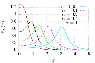
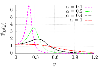
Figure 1: (color online): Exponential decay of the dissipation function $\gamma_{D}(t)=(\gamma_{0}/2\tau_{c})e^{-t/\tau_{c}}$ known as the Drude model. Probability distributions $\mathbb{P}_{D}(x)$ and $\tilde{\mathbb{P}}_{D}(y)$ in two different scalings are shown for selected values of the dimensionless parameter $\alpha=\tau_{v}/\tau_{c}$. In the left panel $\tau_{c}$ is fixed and $\tau_{v}$ is changed. In the right panel $\tau_{v}$ is fixed and $\tau_{c}$ is changed.

III Physical significance of the quantum energy partition theorem

As we write in the Introduction, various expressions for the kinetic energy of a free Brownian particle can be found both in original papers and the well-known books, e.g. Eq. (83) in Ref. hakim , Eq. (4.14) in Ref. ford88 , equation for the second moment of momentum in Table 2 of Ref. ingol1 and Eq. (3.475) in Ref. breuer . The form of $E_{k}$ can also be deduced from the fluctuation-dissipation relation obtained in the framework of the linear response theory which relates relaxation of a weakly perturbed system to the spontaneous fluctuations in thermal equilibrium, see e.g. Eq. (124.10) in Ref. landau , Eq. (17.19g) in Ref. zubarev and Eq. (3.499) in Ref. breuer . All expressions for $E_{k}$ should be equivalent although they are written in different forms. However, our specific formula (10) allows to reveal a new face of the old problem and formulate new interpretations:
I. The mean kinetic energy $E_{k}$ of a free quantum particle equals the average kinetic energy $\langle\mathcal{E}_{k}\rangle$ of the thermostat degree of freedom, i.e. $E_{k}=\langle\mathcal{E}_{k}\rangle$. Mutatis mutandis, the form of this statement is exactly the same as for classical systems: The mean kinetic energy of a free classical particle equals the average kinetic energy of the thermostat degree of freedom.
II. The function $\mathbb{P}(\omega)$ is a probability density, i.e. it is non-negative and normalized on the interval $(0,\infty)$. From the probability theory it follows that there exists a random variable $\xi$ for which $\mathbb{P}(\omega)$ is its probability distribution. Here, this random variable is interpreted as frequency of thermostat oscillators.
III. Eq. (12) can be converted to the transparent form

$$\mathbb{P}(\omega)=\frac{2}{\pi}\,\int_{0}^{\infty}dt\,R(t)\cos(\omega t).$$ (15)

Thus the probability distribution $\mathbb{P}(\omega)$ is a cosine Fourier transform of the response function $R(t)$ which solves the generalized Langevin equation (6).
IV. Thermostat oscillators contribute to $E_{k}$ in a non-uniform way according to the probability distribution $\mathbb{P}(\omega)$. The form of this distribution depends on the response function in which full information on the thermostat modes and system-thermostat interaction is contained.
V. For high temperature, Eq. (11) is approximated by $\mathcal{E}_{k}(\omega)=k_{B}T/2$ and from Eq. (10) we obtain the relation $E_{k}=k_{B}T/2$, i.e. Eq. (10) reduces to the energy equipartition theorem for classical systems.

The next comment concerns the relation of Eq. (10) with the fluctuation-dissipation theorem derived in the linear response theory. We adapt Eq. (124.10) from the Landau-Lifshitz book landau in order to get the kinetic energy of the quantum particle, namely,

$$E_{k}=\frac{1}{2M}\langle p^{2}\rangle=\frac{\hbar}{2\pi M}\int_{0}^{\infty}d\omega\,\coth{\left[\frac{\hbar\omega}{2k_{B}T}\right]}\,\alpha^{\prime\prime}(\omega),$$ (16)

where $\alpha^{\prime\prime}(\omega)$ is the imaginary part of the generalized susceptibility $\alpha(\omega)=\alpha^{\prime}(\omega)+i\alpha^{\prime\prime}(\omega)$. By direct comparison of Eq. (10) and (16) we find the non-trivial relation between the probability distribution and the imaginary part of the generalized susceptibility,

$$\mathbb{P}(\omega)=\frac{2}{\pi}\frac{\alpha^{\prime\prime}(\omega)}{M\omega}.$$ (17)

The second example is Eq. (4.14) in Ref. ford88 :

$$E_{k}=\frac{\hbar}{2\pi}\int_{0}^{\infty}d\omega\,\coth{\left[\frac{\hbar\omega}{2k_{B}T}\right]}\,M\omega^{2}\,\mbox{Im}[\alpha(\omega+i0^{+})],$$ (18)

where $\alpha(\omega)$ is also called susceptibility, which is not the same as in Eq. (16). Again, if we compare Eqs. (10) and (18) then we can find the relation between $\mathbb{P}(\omega)$ and $\mbox{Im}[\alpha(\omega+i0^{+})]$. But now we get

$$\mathbb{P}(\omega)=\frac{2}{\pi}M\omega\,\mbox{Im}[\alpha(\omega+i0^{+})].$$ (19)

We presented only two examples and to avoid confusion the reader should be careful with such relations because they depend on the specific form of the expression for $E_{k}$. Paraphrasing, ”various authors present the same topic differently”.

Overall, taking into account the non-trivial relation between the probability distribution $\mathbb{P}(\omega)$ and the imaginary part of the generalized susceptibility $\alpha^{\prime\prime}(\omega)$ we may say that our principle for quantum partition of energy (10) can be seen as a specific form of the fluctuation-dissipation theorem of the Callen-Welton type although it would be rather difficult to guess the form of $\mathbb{P}(\omega)$ knowing only the formula for fluctuation-dissipation theorem. Finally, we note that Eq. (17) establishes the relation between the probability distribution $\mathbb{P}(\omega)$ and the generalized susceptibility $\alpha^{\prime\prime}(\omega)$. It means that features of the quantum environment described by $\mathbb{P}(\omega)$ may be experimentally inferred from the measurement of the linear response of the system to an applied perturbation given as the corresponding classical susceptibility, e.g. electrical or magnetic. Consequently, according to our results the latter quantity may open a new pathway to study quantum open systems.

IV Analysis of the probability distribution $\mathbb{P}(\omega)$

In the case of classical systems the averaged kinetic energy of the Brownian particle equals $E_{k}=k_{B}T/2$ and all thermostat oscillators have the same averaged kinetic energy $\mathcal{E}_{k}=k_{B}T/2$ which does not depend on the frequency of a single oscillator. In the quantum case, $\mathcal{E}_{k}=\mathcal{E}_{k}(\omega)$ depends on the oscillator frequency $\omega$ and oscillators of various frequencies contribute to $E_{k}$ with various probabilities. Therefore it is interesting to reveal which frequencies are more or less probable in dependence on the dissipation mechanism. The impact of various dissipation mechanisms can be analysed via one of three quantities: the dissipation kernel $\gamma(t)$, the correlation function $C(t)$ of the random force $\eta(t)$ or the spectral density $J(\omega)$. In our view, this mechanism can be intuitively modelled by various forms of the damping kernel $\gamma(t)$. Therefore in the following section we will examine properties of the probability distribution $\mathbb{P}(\omega)$ for several classes of $\gamma(t)$.

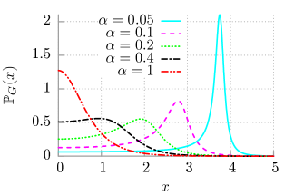
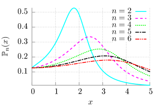
Figure 2: (color online): Left panel: The case of Gaussian decay of the memory kernel $\gamma_{G}(t)=(\gamma_{0}/\sqrt{\pi}\tau_{c})\,\mbox{e}^{-t^{2}/\tau_{c}^{2}}$. Probability distribution $\mathbb{P}_{G}(x)$ is presented for different values of the dimensionless parameter $\alpha$ ($M$ and/or $\gamma_{0}$ is changed, $\tau_{c}$ is fixed). Right panel: The probability distribution $\mathbb{P}_{n}(x)$ is depicted for different values of the power exponent $n$ appearing in the generalized algebraic decay of the dissipation kernel $\gamma_{n}(t)=[(n-1)/2]\,\gamma_{0}\tau_{c}^{n-1}/(t+\tau_{c})^{n}$. The dimensionless parameter $\alpha=0.1$.

IV.1 Drude model

As the first step we assume the dissipation function $\gamma(t)$ to be in the form

$$\gamma_{D}(t)=\frac{\gamma_{0}}{2\tau_{c}}e^{-t/\tau_{c}}$$ (20)

with two non-negative parameters $\gamma_{0}$ and $\tau_{c}$. The first one $\gamma_{0}$ is the particle-thermostat coupling strength and has the unit $[\gamma_{0}]=[kg/s]$, i.e. the same as the friction coefficient in the Stokes force. The second parameter $\tau_{c}$ characterizes time scale on which the system exhibits memory (non-Markovian) effects. Due to fluctuation-dissipation theorem $\tau_{c}$ can be also viewed as the primary correlation time of quantum thermal fluctuations. This exponential form of the memory function is known as a Drude model and it has been frequently considered in coloured noise problems. We choose the above scaling to ensure that if $\tau_{c}\to 0$ the function $\gamma_{D}(t)$ is proportional to the Dirac delta and the integral term in the generalized Langevin equation reduces to the frictional force of the Stokes form. Other damping kernels considered in the later part of this section also possesses this scaling property. With (3), instead of determining $\gamma(t)$, one can equivalently specify the spectral density of thermostat modes which for the Drude damping reads

$$J_{D}(\omega)=\frac{1}{\pi}\frac{\gamma_{0}}{1+\omega^{2}\tau_{c}^{2}}.$$ (21)

From Eq. (14) we get the following expression for the probability density

$$\mathbb{P}(\omega)=\frac{1}{\pi}\,\frac{\mu_{0}\varepsilon^{2}(\omega^{2}+\varepsilon^{2})}{\omega^{2}[\omega^{2}+\varepsilon(\varepsilon-\mu_{0}/2)]^{2}+\mu_{0}^{2}\varepsilon^{4}/4},$$ (22)

where $\mu_{0}=\gamma_{0}/M$ defines the rescaled coupling strength of the Brownian particle to the thermostat and $\varepsilon=1/\tau_{c}$ is the Drude frequency. There are two control parameters $\varepsilon$ and $\mu_{0}$ which have the unit of frequency or equivalently two time scales: the memory time $\tau_{c}$ and $\tau_{v}=M/\gamma_{0}=1/\mu_{0}$ which in the case of a classical free Brownian particle defines the velocity relaxation time.

If we want to analyse the impact of the particle mass $M$ or the coupling $\gamma_{0}$ we should use the following scaling

$$x=\omega\tau_{c}=\frac{\omega}{\varepsilon},$$ (23)

which yields the expression

$$\mathbb{P}_{D}(x)=\varepsilon\mathbb{P}\left(\varepsilon x\right)=\frac{2}{\pi}\,\frac{2\alpha(x^{2}+1)}{x^{2}[2\alpha(x^{2}+1)-1]^{2}+1},$$ (24)

where

$$\alpha=\frac{M}{\tau_{c}\gamma_{0}}=\frac{\varepsilon}{\mu_{0}}=\frac{\tau_{v}}{\tau_{c}}$$ (25)

is the ratio of two characteristic times. It is remarkable that this probability distribution does not depend on these three parameters separately but only on one parameter $\alpha$ being their specific combination. We should remember that $\tau_{c}$ is fixed in this scaling. In Fig. 1 we present the probability distribution $\mathbb{P}_{D}(x)$ for different values of the parameter $\alpha$. We can observe that the thermostat oscillators contribute to the kinetic energy $E_{k}$ in a non-homogeneous way. There is the most probable value of $\mathbb{P}_{D}(x)$ indicating the optimal oscillator frequency $x_{M}$ which brings the greatest contribution to the kinetic energy of the Brownian particle. As it is illustrated in the panel, $x_{M}$ is inversely proportional to $\alpha$: for small values of $\alpha$ mainly oscillators of high frequency contribute to $E_{k}$ whereas for large values of $\alpha$ primarily low frequencies. As $\alpha$ increases $x_{M}\to 0$ and $\mathbb{P}_{D}(x)$ becomes a monotonically decreasing function (not depicted). In other words it means that e.g. when the coupling strength between the system and thermostat $\gamma_{0}$ is strong then contribution of high-frequency oscillators to $E_{k}$ is most pronounced; if the particle mass $M$ increases the optimal frequency $x_{M}$ decreases.

Next we analyse the influence of the memory time $\tau_{c}$ on the probability distribution $\mathbb{P}(\omega)$. For this purpose we should use another scaling:

$$y=\frac{\omega}{\mu_{0}}.$$ (26)

It leads to the expression

$$\tilde{\mathbb{P}}_{D}(y)=\mu_{0}\mathbb{P}(\mu_{0}y)=\frac{1}{\pi}\frac{\alpha^{2}(y^{2}+\alpha^{2})}{y^{2}[y^{2}+\alpha(\alpha-1/2)]^{2}+\alpha^{4}/4},$$ (27)

with the same dimensionless parameter $\alpha$ defined in (25). In the right panel of Fig. 1 we present this distribution for selected values of $\alpha$. It follows that for small values of the parameter $\alpha$, or equivalently for long memory time $\tau_{c}$, the distribution is notably peaked in the region of low frequency modes. Then it rapidly decreases to zero. Consequently only slowly vibrating thermostat oscillators contribute significantly to the kinetic energy of the particle. The situation is quite different for short memory time $\tau_{c}$ (large values of $\alpha$). Then the distribution is flattened meaning that much wider window of oscillators frequency contribute to $E_{k}$ in a similar way.

In the remaining part of the paper, we present the probability distribution $\mathbb{P}(\omega)$ without any scaling. The reader can easily reproduce both scalings. For the scaling as in Eq. (23), one can put $\epsilon=1$ and rescale $\mu_{0}\to\mu_{0}/\varepsilon$ to get the distribution $\mathbb{P}_{i}(x)$ (the index $i$ indicates the form of the memory function). For the scaling as in Eq. (26), one can put $\mu_{0}=1$ and rescale $\varepsilon\to\varepsilon/\mu_{0}$ to get the distribution $\mathbb{P}_{i}(y)$. In the first scaling, one can analyse the influence of the particle mass $M$ and the particle-thermostat coupling $\gamma_{0}$. In the second scaling - the memory time $\tau_{c}$.

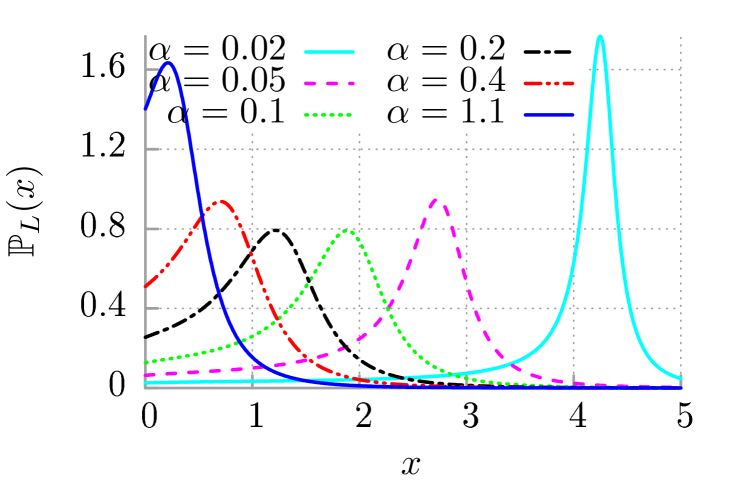
Figure 3: (color online): The probability distribution $\mathbb{P}_{L}(x)$ is depicted for the Lorentzian dissipation kernel $\gamma_{L}(t)=\gamma_{0}\tau_{c}/\pi(t^{2}+\tau_{c}^{2})$ and selected values of the dimensionless parameter $\alpha$ ($M$ or $\gamma_{0}$ can be changed and $\tau_{c}$ is fixed).

IV.2 Gaussian decay

Another possible choice of the dissipation kernel $\gamma(t)$ is the rapidly decreasing Gaussian function, namely,

$$\gamma_{G}(t)=\frac{\gamma_{0}}{\sqrt{\pi}\tau_{c}}\,\mbox{e}^{-t^{2}/\tau_{c}^{2}}$$ (28)

for which the corresponding spectral density is also Gaussian and reads

$$J_{G}(\omega)=\frac{\gamma_{0}}{\pi}\,\mbox{e}^{-\omega^{2}\tau_{c}^{2}/4}.$$ (29)

In order to have an identical notation as in the previous case, we present the probability distribution in the form ($\varepsilon=1/\tau_{c}$)

$$\mathbb{P}_{G}(\omega)=\frac{4}{\pi\mu_{0}}\,\frac{e^{-(\omega/4\varepsilon)^{2}}}{\left[2\omega/\mu_{0}+ie^{-(\omega/4\varepsilon)^{2}}\mbox{Erf}\left(-i\omega/2\varepsilon\right)\right]\left[2\omega/\mu_{0}-ie^{-(\omega/4\varepsilon)^{2}}\mbox{Erf}\left(i\omega/2\varepsilon\right)\right]},$$ (30)

where $\mbox{Erf}(z)$ is the error function

$$\mbox{Erf}(z)=\frac{2}{\sqrt{\pi}}\int_{0}^{z}dt\,e^{-t^{2}}.$$ (31)

In Fig. 2 we present this probability distribution $\mathbb{P}_{G}(x)$ [in the scaling (23)] for selected values of $\alpha$ ($\tau_{v}=M/\gamma_{0}$ is changed and $\tau_{c}$ is fixed) . Similarly as in the case of the Drude model, the oscillator frequency $x_{M}$ which brings the greatest contribution to the kinetic energy of the particle is inversely proportional to the parameter $\alpha$. However, here we observe two differences: (i) at some interval of $\alpha$ the maximum of $\mathbb{P}_{G}(x)$ decreases as $\alpha$ increases and (ii) the half-width of $\mathbb{P}_{G}(x)$ increases as $\alpha$ increases while for the Drude model it is almost constant in a wide interval of $\alpha$. In this case, the impact of the memory time $\tau_{c}$ is similar to that as for the Drude dissipation, see the right panel of Fig. 1.

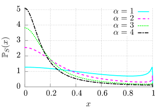
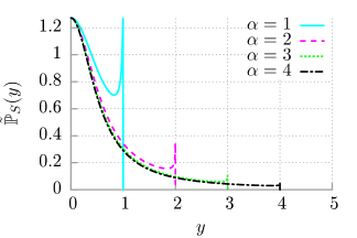
Figure 4: (color online): The probability distribution $\mathbb{P}_{S}(x)$ is presented for the oscillatory decay $\gamma_{S}(t)=(\gamma_{0}/\pi)\sin(t/\tau_{c})/t$ (the Debye type model) and selected values of the dimensionless parameter $\alpha=\tau_{v}/\tau_{c}$. In the left panel $\tau_{c}$ is fixed and $\tau_{v}=M/\gamma_{0}$ is changed. In the right panel $\tau_{v}$ is fixed and $\tau_{c}$ is changed.

IV.3 n-Algebraic decay

Apart from two exponential forms of the memory functions which we presented above one could model the dissipation function $\gamma(t)$ with algebraic decay. It is worth noting that the power-law decay of the memory functions has been considered as a model of anomalous transport processes anomal1 ; anomal2 . Here, we consider the class of functions

$$\gamma_{n}(t)=\frac{n-1}{2}\frac{\gamma_{0}\tau_{c}^{n-1}}{(t+\tau_{c})^{n}},$$ (32)

where $n\in\mathbb{N}$ and $n\geq 2$. It has the same limiting Dirac delta form for $\tau_{c}\to 0$ as in two previous cases. The corresponding spectral density reads

$$J_{n}(\omega)=\frac{(n-1)\gamma_{0}}{2\pi}\,\left[e^{-i\omega\tau_{c}}E_{n}(-i\omega\tau_{c})+e^{i\omega\tau_{c}}E_{n}(i\omega\tau_{c})\right]$$ (33)

and $E_{n}(z)$ is the exponential integral,

$$E_{n}(z)=\int_{1}^{\infty}dt\,\frac{e^{-zt}}{t^{n}}.$$ (34)

The probability distribution takes the form

$$\mathbb{P}_{n}(\omega)=\frac{2(n-1)}{\pi\mu_{0}}\frac{e^{-i\omega/\varepsilon}E_{n}(-i\omega/\varepsilon)+e^{i\omega/\varepsilon}E_{n}(i\omega/\varepsilon)}{\left[(n-1)e^{-i\omega/\varepsilon}E_{n}(-i\omega/\varepsilon)-2i\omega/\mu_{0}\right]\left[(n-1)e^{i\omega/\varepsilon}E_{n}(i\omega/\varepsilon)+2i\omega/\mu_{0}\right]}.$$ (35)

In Fig. 2 we present the influence of the power exponent $n$ appearing in the dissipation function $\gamma_{n}(t)$ on the probability distribution $\mathbb{P}_{n}(x)$ for fixed $\alpha=0.1$. The conclusion is: an increase of the exponent $n$ causes progressive flattening of the probability density function. In other words, if the memory function decreases faster and faster to zero the wider spectrum of frequencies of the thermostat oscillators contribute to $E_{k}$.

IV.4 Lorentzian decay

It is interesting to compare the algebraic case for $n=2$ with the Lorentzian memory function which reads

$$\gamma_{L}(t)=\frac{\gamma_{0}}{\pi}\,\frac{\tau_{c}}{t^{2}+\tau_{c}^{2}}.$$ (36)

In the probability theory it is termed as the Cauchy distribution. Alternatively, it may be imposed by the following spectral density of thermostat modes,

$$J_{L}(\omega)=\frac{\gamma_{0}}{\pi}e^{-\omega\tau_{c}}.$$ (37)

Such a choice of the dissipation kernel leads to the following probability distribution ($\varepsilon=1/\tau_{c}$)

$$\mathbb{P}_{L}(\omega)=\frac{4\pi}{\mu_{0}}\,\frac{e^{-\omega/\varepsilon}}{\pi^{2}e^{-2\omega/\varepsilon}+c^{2}(\omega)},$$ (38)

where

$$c(\omega)=e^{-\omega/\varepsilon}\mbox{Ei}(\omega/\varepsilon)-e^{\omega/\varepsilon}\mbox{Ei}(-\omega/\varepsilon)-\frac{2\pi}{\mu_{0}}\omega$$ (39)

and $\mbox{Ei}(z)$ is the exponential integral defined as

$$\mbox{Ei}(z)=\int_{-\infty}^{z}\frac{e^{t}}{t}\,dt.$$ (40)

We illustrate this probability distribution in Fig. 3 for different values of the dimensionless parameter $\alpha=M/\tau_{c}\gamma_{0}$. The oscillator frequency $x$ which brings the greatest contribution to the kinetic energy of the particle is inversely proportional to the parameter $\alpha$. Again, as it was in the previous cases, the magnitude of the maxima in the probability distribution $\mathbb{P}_{L}(x)$ also depends on $\alpha$. For very small values of $\alpha$ one can note that high frequency modes almost exclusively contribute to the kinetic energy of the particle.

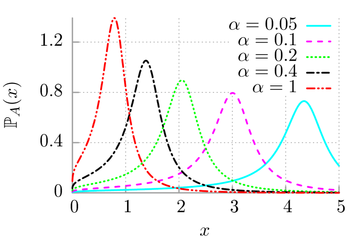
Figure 5: (color online): Algebraic decay of the dissipation function $\gamma_{A}(t)=\gamma_{0}/(t+\tau_{c})$. Probability distribution $\mathbb{P}_{A}(x)$ is presented for different values of the dimensionless parameter $\alpha$.

IV.5 Debye type model: Algebraically decaying oscillations

The next example of this series is the oscillatory memory function zwan

$$\gamma_{S}(t)=\frac{\gamma_{0}}{\pi}\frac{\sin{(t/\tau_{c})}}{t}.$$ (41)

which takes both positive and negative values. One can show that, via the fluctuation-dissipation relation, the quantum noise $\eta(t)$ exhibits anti-correlations. The spectral density is of the Debye type zwan

$$J_{S}(\omega)=\frac{\gamma_{0}}{\pi}\,\theta\left(\frac{1}{\tau_{c}}-\omega\right),$$ (42)

where $\theta(x)$ denotes the Heaviside step function. This spectral density is constant $J(\omega)=\gamma_{0}/\pi$ on the compact support $[0,1/\tau_{c}]$ determined by the memory time $\tau_{c}$ or the cut-off frequency $\varepsilon=1/\tau_{c}$. Under this assumption the probability density $\mathbb{P}_{S}(\omega)$ reads

$$\mathbb{P}_{S}(\omega)=\frac{4\pi}{\mu_{0}}\,\frac{\theta(\varepsilon-\omega)}{\pi^{2}(1+4\omega^{2}/\mu_{0}^{2})+4\mbox{arctanh}(\omega/\varepsilon)[\mbox{arctanh}(\omega/\varepsilon)-2\pi\omega/\mu_{0}]}$$ (43)

and has the same support as $J(\omega)$ in the interval $[0,\varepsilon]$. In Fig. 4 we present the probability density $\mathbb{P}_{S}(x)$ for selected values of the dimensionless parameter $\alpha$ in two various scalings. In the left panel, the memory time is fixed and the coupling $\gamma_{0}$ or the mass $M$ is changed. Again, when e.g. $\gamma_{0}$ decreases (i.e. $\alpha$ increases) more and more oscillators of low frequency contribute to $E_{k}$.

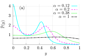
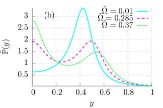
Figure 6: (color online): Panel (a): The probability distribution $\tilde{\mathbb{P}}(y)$ scaled according to Equation (26) is depicted for exponentially decaying oscillations with $\gamma_{E}(t)=(\gamma_{0}/\tau_{c})e^{-t/\tau_{c}}\cos{(\Omega t)}$ and different values of $\alpha=\varepsilon/\mu_{0}$ and fixed $\tilde{\Omega}=\Omega/\mu_{0}=0.285$. Panel (b): The same $\tilde{\mathbb{P}}(y)$ is presented for selected dimensionless frequencies $\tilde{\Omega}$ of the memory function and fixed $\alpha=0.2$.

IV.6 Slow algebraic decay

In this subsection we consider slow algebraic decay of the memory kernel assuming

$$\gamma_{A}(t)=\frac{\gamma_{0}}{t+\tau_{c}}.$$ (44)

This dissipation function does not tend to the Dirac delta when $\tau_{c}\to 0$ (the limit does not exist at all) and therefore is not placed in the subsection IVC. The corresponding spectral density has the form

$$J_{A}(\omega)=\frac{2\gamma_{0}}{\pi}\,a(\omega).$$ (45)

The probability distribution reads

$$\mathbb{P}_{A}(\omega)=\frac{2}{\pi\mu_{0}}\,\frac{a(\omega)}{a^{2}(\omega)+[b(\omega)-\omega/\mu_{0}]^{2}},$$ (46)

where ($\varepsilon=1/\tau_{c}$)

$$a(\omega)=-\mbox{ci}(\omega/\varepsilon)\cos(\omega/\varepsilon)-\mbox{si}(\omega/\varepsilon)\sin(\omega/\varepsilon),$$ (47)

$$b(\omega)=\mbox{ci}(\omega/\varepsilon)\sin(\omega/\varepsilon)-\mbox{si}(\omega/\varepsilon)\cos(\omega/\varepsilon).$$ (48)

The functions $\mbox{ci}(z)$ and $\mbox{si}(z)$ are cosine and sine integrals defined as

$$\mbox{ci}(z) = -\int_{z}^{\infty}\frac{\cos{t}}{t}\,dt,$$ (49)

$$\mbox{si}(z) = -\int_{z}^{\infty}\frac{\sin{t}}{t}\,dt.$$ (50)

In Fig. 5 we depict $\mathbb{P}_{A}(x)$ for different values of the dimensionless parameter $\alpha$. The same as before, the optimal frequency of oscillator which has the largest impact on the kinetic energy is inversely proportional to $\alpha$. Qualitatively, it looks similar to the case of the Drude model, c.f. Fig. 1. However, only for large value of $\alpha$ contribution of harmonic modes of lowest frequency $x\to 0$ differs significantly from zero.

Overall, the common characteristic feature of all cases presented above is that the probability distribution $\mathbb{P}(x)$ occurring in the quantum law for energy equipartition depends only on one dimensionless parameter $\alpha=M/\tau_{c}\gamma_{0}$. Moreover, for a small value of this parameter (the strong particle-thermostat coupling) one typically finds the bell-shaped probability density with a pronounced maximum for high frequency $x_{M}$ which is inversely proportional to the magnitude of $\alpha$. For large value of $\alpha$, thermostat oscillators of low frequency dominate in contribution to the kinetic energy of the Brownian particle.

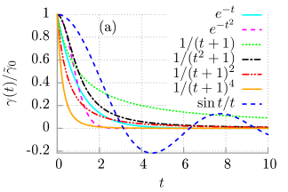
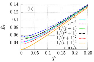
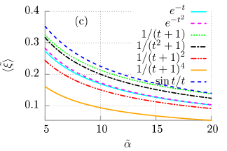
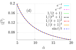
Figure 7: (color online): Panel (a): The normalized memory functions $\gamma(t)/\tilde{\gamma}_{0}$ representing various dissipation mechanisms. Panel (b): The dimensionless kinetic energy $\tilde{E}_{k}=\tau_{c}{E}_{k}/\hbar$ of the free Brownian particle presented versus dimensionless temperature $\tilde{T}=\tau_{c}k_{B}T/\hbar$ and various forms of $\gamma(t)$. Panel (c): The first moment $\langle\tilde{\xi}\rangle=\tau_{c}\langle\xi\rangle$ and panel (d): the second moment $\langle\tilde{\xi}^{2}\rangle=\tau_{c}^{2}\langle\xi^{2}\rangle$ depicted versus the dimensionless parameter $\tilde{\alpha}=M/\tilde{\gamma}_{0}\tau_{c}^{2}$ for different variants of the damping kernel $\gamma(t)$.

IV.7 Exponentially decaying oscillations

As the last example, we consider a generalization of the Drude model in the form of exponentially decaying oscillations bialas ,

$$\gamma_{E}(t)=\frac{\gamma_{0}}{\tau_{c}}e^{-t/\tau_{c}}\cos{(\Omega t)},$$ (51)

where in addition to the previously defined parameters $\gamma_{0}$ and $\tau_{c}$, now $\Omega$ is the frequency in the relaxation process of the particle momentum. Also in this case, the quantum noise $\eta(t)$ exhibits anti-correlations. The limiting case $\Omega=0$ corresponds to the Drude model of dissipation. Such a choice of the damping kernel leads to the following spectral density

$$J_{E}(\omega)=\frac{2}{\pi}\frac{\gamma_{0}\varepsilon^{2}(\varepsilon^{2}+\omega^{2}+\Omega^{2})}{(\varepsilon^{2}+\omega^{2})^{2}+2\Omega^{2}(\varepsilon^{2}-\omega^{2})+\Omega^{2}},$$ (52)

where $\varepsilon=1/\tau_{c}$. From the quantum law for the partition of energy we obtain the probability distribution in the form bialas

$$\mathbb{P}(\omega)=\frac{2}{\pi}\,\frac{\mu_{0}\varepsilon^{2}\left(\omega^{2}+\varepsilon^{2}+\Omega^{2}\right)}{\omega^{2}\left[(\omega^{2}+\varepsilon^{2}-\Omega^{2}-\mu_{0}\varepsilon)^{2}+4\varepsilon^{2}\Omega^{2}\right]+\mu_{0}^{2}\varepsilon^{4}}.$$ (53)

The parameter $\mu_{0}=\gamma_{0}/M$ defines the rescaled coupling strength of the Brownian particle to thermostat. We note that in the considered case there are three characteristic frequencies $\mu_{0}$, $\varepsilon$ and $\Omega$ or equivalently three time scales which are equal to the reciprocals of these frequencies. This observation must be contrasted with all previously considered damping kernels leading to two characteristic time scales. The kinetic energy of the free Brownian particle with the exponentially decaying oscillations in the dissipation function was analysed in detail in Ref. bialas . Instead, here we focus on the properties of the probability density occurring in the quantum energy partition theorem. The influence of the coupling strength $\mu_{0}$ on $\mathbb{P}(\omega)$ is similar to that of the Drude model: there is only one maximum for a fixed value of the coupling strength $\mu_{0}$. For larger values of the latter it is shifted to the right indicating that oscillators of the higher frequency bring the greatest contribution to the kinetic energy of the particle.

The influence of the reciprocal of the correlation time $\varepsilon=1/\tau_{c}$ is depicted in Fig. 6(a). In this case, we scale Eq. (53) as in (26), namely $y=\omega/\mu_{0}$. The dimensionless parameters are $\alpha=\varepsilon/\mu_{0}$ and $\tilde{\Omega}=\Omega/\mu_{0}$. Due to the interplay of two characteristic time scales associated with the parameters $\alpha$ and $\tilde{\Omega}$ we observe here qualitatively new features. For large values of $\alpha\gg\tilde{\Omega}$ the distribution is almost flat indicating that all oscillators of thermostat contribute equally to the kinetic energy of the system. When the the characteristic frequency $\alpha$ is slightly larger than the other one $\alpha>\tilde{\Omega}$ a single maximum is born. When the opposite situation occurs, i.e. $\alpha<\tilde{\Omega}$ then the distribution $\tilde{\mathbb{P}}(y)$ exhibits a clear bimodal character. It means that both oscillators of low and moderate frequency play important role. Further decrease of $\alpha$ extinguishes the contribution of higher frequencies at the favour of the near zero frequency modes which are then the most pronounced ones.

Last but not least, we elaborate on the impact of the oscillation frequency $\Omega$. We keep the scaling with respect to the system-thermostat coupling strength $\mu_{0}$. In Fig. 6(b) we present the probability distribution $\tilde{\mathbb{P}}(y)$ for a few values of the dimensionless frequency $\tilde{\Omega}=\Omega/\mu_{0}$ and fixed $\alpha=\varepsilon/\tau_{c}=0.2$. The result confirms our earlier observation that due to interplay of two characteristic time scales the probability density may be bimodal. It is realized when the magnitude of $\tilde{\Omega}$ and $\alpha$ is comparable. For very small $\tilde{\Omega}$ the distribution $\tilde{\mathbb{P}}(y)$ possesses one very pronounced maximum, whereas for large $\tilde{\Omega}$ it becomes a monotonically decreasing function of the dimensionless frequency $y$.

V Statistical moments of the probability distribution $\mathbb{P}(\omega)$

Let us now discuss statistical moments of the random variable $\xi$ distributed according to the probability density $\mathbb{P}(\omega)$,

$$\langle\xi^{n}\rangle=\int_{0}^{\infty}d\omega\,\omega^{n}\mathbb{P}(\omega).$$ (54)

A caution is needed since not all moments may exist, e.g. for the distribution (22). The first two of them have a clear physical interpretation arxiv2018 . The first moment, i.e. the mean value $\langle\xi\rangle$ of the random variable $\xi$ is proportional to the kinetic energy $E_{k}$ of the Brownian particle at zero temperature $T=0$, namely,

$$E_{0}=E_{k}(T=0)=\frac{\hbar}{4}\,\langle\xi\rangle.$$ (55)

The second moment $\langle\xi^{2}\rangle$ is proportional to the first correction of kinetic energy $E_{k}$ in the high temperature regime,

$$E_{k}=\frac{1}{2}k_{B}T+\frac{\hbar^{2}}{24k_{B}T}\,\langle\xi^{2}\rangle.$$ (56)

We note that averaged kinetic energy $E_{0}$ at zero temperature $T=0$ is non-zero for all values of the system parameters. It is so because of intrinsic quantum vacuum fluctuations. Moreover, $E_{k}$ monotonically increases from some non-zero value to infinity when temperature goes to infinity. If we want to compare impact of various dissipation mechanisms on $E_{k}$ we have to change the scaling of all dissipation functions $\gamma(t)$. Now, we re-define $\gamma(t)$ in such a way that for all memory functions $\gamma(0)=\tilde{\gamma}_{0}$, where $\tilde{\gamma}_{0}$ still characterizes the particle-thermostat coupling but now it has the unit $[\tilde{\gamma}_{0}]=[kg/s^{2}]$. E.g. for the Drude model $\gamma_{D}(t)=\tilde{\gamma}_{0}\,\mbox{exp}(-t/\tau_{c})$ or for the Lorenzian shape $\gamma_{L}(t)=\tilde{\gamma}_{0}/[(t/\tau_{c})^{2}+1]$, see panel (a) of Fig. 7, where all $\gamma(t)$ assume the same value for $t=0$. In the classical case, it would correspond to the fixing of the second moment of the random force $\eta(t)$. In Section 6, we define $\gamma(t)$ in such a way that $\gamma(t)$ tends to the Dirac delta when the memory time $\tau_{c}\to 0$, which in the classical case corresponds to Gaussian white noise of the random force $\eta(t)$.

In Fig. 7(b) we compare the kinetic energy $E_{k}$ for different forms of the memory function $\gamma(t)$. The various curves $E_{k}$ versus temperature never intersect each other for the same set of parameters. Therefore it is sufficient to analyse the energy only at zero temperature $E_{0}\propto\langle\xi\rangle$. We present this characteristic in Fig. 7(c) where we depict the dimensionless first moment $\langle\tilde{\xi}\rangle=\tau_{c}\langle\xi\rangle$ of the probability density $\mathbb{P}(\omega)$ versus the dimensionless parameter $\tilde{\alpha}=M/\tilde{\gamma}_{0}\tau_{c}^{2}$. In calculations we scale $\omega=x/\tau_{c}$ like in (23) with fixed $\tau_{c}$. First, we note that in all cases the averaged kinetic energy at zero temperature decreases when the parameter $\tilde{\alpha}$ increases. We recall that it translates to either (i) increase of the particle mass $M$ or (ii) decrease of the coupling strength $\tilde{\gamma}_{0}$. Moreover, we can see that for the n-algebraic decay ($n=4$ for green and $n=2$ for red curves, respectively) the kinetic energy at zero temperature $E_{0}$ is smaller than for other memory functions. The negligible difference is observed for the Drude and Gaussian decay. The largest kinetic energy is induced by the Debye type dissipation. In the high temperature regime (panel (d) of Figure 7), the correction $\langle\tilde{\xi}^{2}\rangle=\tau_{c}^{2}\langle\xi^{2}\rangle$ depends very weakly on the form of $\gamma(t)$ and the differences are indistinguishable. Finally, at $T=0$, the energy $E_{0}$ increases starting from zero for $\tau_{c}\to 0$ and saturates to a finite value as $\tau_{c}$ is longer and longer (not depicted).

VI Summary

In this work we have revisited an archetype model of quantum Brownian motion formulated in terms of the generalized quantum Langevin equation for a free particle interacting with a large number of independent oscillators that form thermal reservoir. In particular, we analysed the impact of various dissipation mechanisms on the averaged kinetic energy $E_{k}$ of the Brownian particle. For this purpose we harvested the recently formulated quantum law for partition of energy. It expresses the kinetic energy $E_{k}$ of the particle as the mean kinetic energy per one degree of freedom of the thermostat oscillators $E_{k}=\langle\mathcal{E}_{k}\rangle$. The averaging over frequencies $\omega$ of those oscillators is performed according to the probability distribution $\mathbb{P}(\omega)$ which is related to the dissipation kernel $\gamma(t)$ via the quantum partition theorem. We focused mainly on the influence of the form of the dissipation function on characteristic features of the probability density $\mathbb{P}(\omega)$.

We analysed multitude of dissipation mechanisms which are grouped into two classes of the algebraic and exponential decay. Within each of them we considered the monotonic as well as oscillating decay. For the dissipation functions possessing two characteristic time scales associated with the relaxation time of the particle momentum $M/\gamma_{0}$ and the correlation time of quantum thermal fluctuations $\tau_{c}$ typically we observed the bell shaped probability distribution $\mathbb{P}(\omega)$. It means that there is an optimal oscillator frequency which brings the greatest contribution to the kinetic energy of the particle. The magnitude of this optimum is inversely proportional to the system-thermostat coupling strength $\gamma_{0}$. For large values of the latter the contribution of high frequency oscillators is most pronounced. We studied also impact of the memory time $\tau_{c}$ on the shape of the distribution $\mathbb{P}(\omega)$. For long memory time $\tau_{c}$ the probability density is noticeable peaked whereas for short $\tau_{c}$ the distribution is almost flat. Consequently, a decrease of the memory time $\tau_{c}$ causes flattening of the probability density $\mathbb{P}(\omega)$. In this class of dissipation functions we have considered a peculiar case of the algebraically decaying oscillations $\gamma(t)\propto\sin{t}/t$. This choice leads to the distribution $\mathbb{P}(\omega)$ possessing a finite cut-off frequency which curiously depends on the correlation time of quantum fluctuations $\tau_{c}$. For dissipation mechanism with additional characteristic time scale associated with the period of oscillations $2\pi/\Omega$ qualitatively new features emerge in the density $\mathbb{P}(\omega)$. We exemplify this observation for the case of exponentially decaying oscillations. When the magnitude of $\tau_{c}$ and $2\pi/\Omega$ are similar then the probability distribution displays the bimodal character. This means that there are two characteristic frequencies of the thermostat oscillators which brings the significant contribution to the kinetic energy of the system.

We have demonstrated that the quantum law for energy partition in the present formulation is conceptually simple yet very powerful tool for analysis of quantum open systems. We hope that our work will stimulate its further successful applications.

Appendix A Solution of the Langevin equation (6)

Eq. (6) is a linear integro-differential equation for the momentum operator $p(t)$. Because its integral part is a convolution, it can be solved by the Laplace transform method yielding

$$z\hat{p}_{L}(z)-p(0)+\frac{1}{M}\hat{\gamma}_{L}(z)\hat{p}_{L}(z)=-\hat{\gamma}_{L}(z)x(0)+\hat{\eta}_{L}(z),$$ (57)

where $\hat{p}_{L}(z)$, $\hat{\gamma}_{L}(z)$ and $\hat{\eta}_{L}(z)$ are the Laplace transforms of $p(t),\gamma(t)$ and $\eta(t)$, respectively (see Eq. (9). The operators $p(0)$ and $x(0)$ are the momentum and coordinate operators of the Brownian particle at time $t=0$. From this equation it follows that

$$\hat{p}_{L}(z)=\hat{R}_{L}(z)p(0)-\hat{R}_{L}(z)\hat{\gamma}_{L}(z)x(0)+\hat{R}_{L}(z)\hat{\eta}_{L}(z),$$ (58)

where

$$\hat{R}_{L}(z)=\frac{M}{Mz+\hat{\gamma}_{L}(z)}.$$ (59)

The inverse Laplace transform of (58) gives the solution $p(t)$ for the momentum of the Brownian particle, namely,

$$p(t) =R(t)p(0)-\int_{0}^{t}du\;R(t-u)\gamma(u)x(0)$$

$$+\int_{0}^{t}du\;R(t-u)\eta(u),$$ (60)

where the response function $R(t)$ is the inverse Laplace transform of the function $\hat{R}_{L}(z)$ in Eq. (59). Because statistical properties of thermal noise $\eta(t)$ are specified, all statistical characteristics of the particle momentum $p(t)$ can be calculated, in particular its kinetic energy.

Appendix B Kinetic energy in an equilibrium state

In order to derive the averaged kinetic energy of the Brownian particle in the equilibrium state, we first calculate the symmetrized momentum-momentum correlation function $\left<\left[p(t);p(s)\right]_{+}\right>$. For long times, $t\gg 1,s\gg 1$, only the last term of (A) contributes and then

$$\left<\left[p(t);p(s)\right]_{+}\right>=\int_{0}^{t}dt_{1}\int_{0}^{s}dt_{2}\;R(t-t_{1})R(s-t_{2})\left<\left[\eta(t_{1});\eta(t_{2})\right]_{+}\right>.$$ (61)

Now, we express the correlation function $C(t_{1}-t_{2})=\left<\left[\eta(t_{1});\eta(t_{2})\right]_{+}\right>$ of quantum thermal noise by its Fourier transform, see Eq. (76b) in Appendix C,

$$\left<\left[p(t);p(s)\right]_{+}\right>=\int_{0}^{\infty}d\omega\;\hat{C}_{F}(\omega)\int_{0}^{t}dt_{1}\int_{0}^{s}dt_{2}\;R(t-t_{1})R(s-t_{2})\cos\left[\omega\left(t_{1}-t_{2}\right)\right].$$ (62)

In particular, for $t=s$, it is the second statistical moment of the momentum,

$$\langle p^{2}(t)\rangle=\int_{0}^{\infty}d\omega\;\hat{C}_{F}(\omega)\int_{0}^{t}dt_{1}\int_{0}^{t}dt_{2}\;R(t-t_{1})R(t-t_{2})\cos\left[\omega\left(t_{1}-t_{2}\right)\right].$$ (63)

We introduce new integration variables $\tau=t-t_{1}$ and $u=t-t_{2}$ and convert equation (63) into the form

$$\langle p^{2}(t)\rangle=\int_{0}^{\infty}d\omega\;\hat{C}_{F}(\omega)\int_{0}^{t}d\tau\int_{0}^{t}du\;R(\tau)R(u)\cos\left[\omega\left(\tau-u\right)\right].$$ (64)

We perform the limit $t\to\infty$ to derive an expression for the average kinetic energy in the equilibrium state, namely,

$$E_{k}=\lim_{t\to\infty}\frac{1}{2M}\langle p^{2}(t)\rangle=\frac{1}{2M}\int_{0}^{\infty}d\omega\;\hat{C}_{F}(\omega)I(\omega),$$ (65)

where

$$I(\omega) =\int_{0}^{\infty}d\tau\int_{0}^{\infty}du\;R(\tau)R(u)\cos\left[\omega\left(\tau-u\right)\right]$$

$$=\hat{R}_{L}(i\omega)\hat{R}_{L}(-i\omega)$$ (66)

is the product of a Laplace transform of the response function $R(t)$. At this point, we can exploit the fluctuation-dissipation relation (78) (Appendix C) to express the noise correlation spectrum $\hat{C}_{F}(\omega)$ by the dissipation spectrum $\hat{\gamma}_{F}(\omega)$ and convert (65) to the form

$$E_{k}=\int_{0}^{\infty}d\omega\;\frac{\hbar\omega}{4M}\coth\left({\frac{\hbar\omega}{2k_{B}T}}\right)\;\hat{\gamma}_{F}(\omega)\hat{R}_{L}(i\omega)\hat{R}_{L}(-i\omega).$$ (67)

We observe that

$$\mathcal{E}_{k}(\omega)=\frac{\hbar\omega}{4}\coth\left({\frac{\hbar\omega}{2k_{B}T}}\right)$$ (68)

is averaged (thermal) kinetic energy per one degree of freedom of the thermostat consisting of free harmonic oscillators feynman . The remaining part of the integrand in Eq. (67) reads

$$\mathbb{P}(\omega) = \frac{1}{M}\hat{\gamma}_{F}(\omega)\hat{R}_{L}(i\omega)\hat{R}_{L}(-i\omega)$$ (69)

$$= \frac{M}{\pi}\frac{\hat{\gamma}_{L}(i\omega)+\hat{\gamma}_{L}(-i\omega)}{[\hat{\gamma}_{L}(i\omega)+iM\omega][\hat{\gamma}_{L}(-i\omega)-iM\omega]}$$

$$= \frac{1}{\pi}\left[\hat{R}_{L}(i\omega)+\hat{R}_{L}(-i\omega)\right],$$

where we used Eq. (59) for $\hat{R}_{L}(z)$ and the relation between the Laplace and cosine Fourier transforms. With these two expressions for $\mathcal{E}_{k}(\omega)$ and $\mathbb{P}(\omega)$, the final form of the averaged kinetic energy $E_{k}$ of the Brownian particle reads

$$E_{k}=\int_{0}^{\infty}d\omega\;\mathcal{E}_{k}(\omega)\mathbb{P}(\omega).$$ (70)

Appendix C Fluctuation-dissipation relation

We assume the factorized initial state of the composite system, i.e., $\rho(0)=\rho_{S}\otimes\rho_{E}$, where $\rho_{S}$ is an arbitrary state of the Brownian particle and $\rho_{E}$ is an equilibrium canonical state of the thermostat of temperature $T$, namely,

$$\rho_{E}=\mbox{exp}(-H_{E}/k_{B}T)/\mbox{Tr}[\mbox{exp}(-H_{E}/k_{B}T)],$$ (71)

where:

$$H_{E}=\sum_{i}\left[\frac{p_{i}^{2}}{2m_{i}}+\frac{1}{2}m_{i}\omega_{i}^{2}q_{i}^{2}\right]$$ (72)

is the Hamiltonian of the thermostat. The factorization means that there are no initial correlations between the particle and the thermostat. The initial preparation turns the force $\eta(t)$ into the operator-valued quantum thermal noise which in fact is a family of non-commuting operators whose commutators are $c$-numbers. This noise is unbiased and its mean value is zero,

$$\langle\eta(t)\rangle\equiv\mbox{Tr}\left[\eta(t)\rho_{E}\right]=0.$$ (73)

Its symmetrized correlation function

$$C(t,u)=\left<\left[\eta(t);\eta(u)\right]_{+}\right>=\frac{1}{2}\langle\eta(t)\eta(u)+\eta(u)\eta(t)\rangle$$ (74)

depends on the time difference

$$C(t,u) =C(t-u)$$

$$=\sum_{i}\frac{\hbar c_{i}^{2}}{2m_{i}\omega_{i}}\coth\left(\frac{\hbar\omega_{i}}{2k_{B}T}\right)\cos[\omega_{i}(t-u)]$$

$$=\int_{0}^{\infty}d\omega\,\frac{\hbar\omega}{2}\coth\left(\frac{\hbar\omega}{2k_{B}T}\right)J(\omega)\cos[\omega(t-u)],$$ (75)

where the spectral function $J(\omega)$ is given by Eq. (4). The higher order correlation functions are expressed by $C(t_{i}-t_{j})$ and have the same form as statistical characteristics for classical stationary Gaussian stochastic processes. Therefore $\eta(t)$ defines a quantum stationary Gaussian process with time homogeneous correlations.

The dissipation and correlation functions can be presented as cosine Fourier transforms

$$\gamma(t)=\int_{0}^{\infty}d\omega\,\hat{\gamma}_{F}(\omega)\cos(\omega t),$$ (76a)

$$C(t)=\int_{0}^{\infty}d\omega\,\hat{C}_{F}(\omega)\cos(\omega t),$$ (76b)

with their inverse

$$\hat{\gamma}_{F}(\omega)=\frac{2}{\pi}\int_{0}^{\infty}dt\,\gamma(t)\cos(\omega t),$$ (77a)

$$\hat{C}_{F}(\omega)=\frac{2}{\pi}\int_{0}^{\infty}dt\,C(t)\cos(\omega t),$$ (77b)

If we compare Eqs. (3) and (C)-(76b) then we observe that

$$\hat{C}_{F}(\omega)=\frac{\hbar\omega}{2}\coth\left(\frac{\hbar\omega}{2k_{B}T}\right)\,\hat{\gamma}_{F}(\omega).$$ (78)

This relation between the spectrum $\hat{\gamma}_{F}(\omega)$ of dissipation and the spectrum $\hat{C}_{F}(\omega)$ of thermal noise correlations is the body of the fluctuation-dissipation theorem call ; kub in which quantum effects are incorporated via the prefactor in r.h.s. of Eq. (78). We want to pay attention that the definition (4) of the spectral density $J(\omega)$ differs from another frequently used form $\tilde{J}(\omega)=\omega J(\omega)$. We prefer the definition (4) because of a direct relation to the Fourier transforms of (3) and (76a), i.e. $J(\omega)=\hat{\gamma}_{F}(\omega)$. Here, the Ohmic case corresponds to $J(\omega)=$const.

For a finite number of the thermostat oscillators, all dynamical quantities are almost periodic functions of time, in particular the dissipation function $\gamma(t)$ and the correlation function $C(t)$. In the thermodynamic limit, when a number of oscillators tends to infinity, the dissipation function $\gamma(t)$ decays to zero as $t\to\infty$ and the singular spectral function $J(\omega)$ defined by Eq. (4) tends to a (piecewise) continuous function. In such a point of view, dissipation mechanism is determined by the memory kernel $\gamma(t)$ or equivalently by the spectral density of thermostat modes $J(\omega)$ which contains necessary information on the particle-thermostat interaction.

References

- (1) K. Huang, Statistical mechanics (Wiley, New York, 1987)
- (2) Y. P. Terletskií Statistical Physics (North-Holland, Amsterdam, The Netherlands, 1971)
- (3) V. Hakim, V. Ambegaokar, Phys. Rev. A 32, 423 (1985)
- (4) G. W. Ford, J. T. Lewis, R. F. O’Connell, Phys. Rev. Lett. 55, 2273 (1985)
- (5) G. W. Ford, J. T. Lewis, R. F. O’Connell, Ann. Phys. (N.Y.) 185, 270 (1988)
- (6) H. Grabert, P. Schramm, G. L. Ingold, Phys. Rep. 168, 115 (1988)
- (7) U. Weiss, Quantum Dissipative Systems (World Scientific: Singapore, 2008)
- (8) L. D. Landau, E. M. Lifshitz Statistical Physics, Part 1 (Butterworth-Heinemann, 3rd ed., 1980)
- (9) D. N. Zubarev, Nonequilibrium statistical thermodynamics (New York, Consultants Bureau, 1974)
- (10) H. P. Breuer and F. Petruccione, The theory of open quantum systems (New York, Oxford University Press, 2002).
- (11) J. Grela, S. N. Majumdar and G. Scherer, Phys. Rev. Lett. 119, 130601 (2017)
- (12) P. Massignan, A. Lampo, J. Wehr and M. Lewenstein, Phys. Rev. A 91, 033627 (2015)
- (13) J. Tuziemski and J. K. Korbicz, EPL 112, 40008 (2015)
- (14) L. Ferialdi and A. Smirne, Phys. Rev. A 96, 012109 (2017)
- (15) D. Boyanovsky and D. Jasnow, Phys. Rev. A 96, 062108 (2017)
- (16) B. Jack, J. Senkpiel, M. Etzkorn, J. Ankerhold, Ch. Ast and K. Kern, Phys. Rev. Lett. 119, 147702 (2017)
- (17) M. Carlesso, A. Bassi, Phys. Rev. A 95, 052119 (2017)
- (18) S. H. Lim, J. Wehr, A. Lampo, M. A. Garica-March, and M. Lewenstein, J. Stat. Phys. 170, 351 (2018)
- (19) H. Z. Shen, S. L. Su, Y. H. Zhou and X. X. Yi, Phys. Rev. A 97, 042121 (2018)
- (20) A. Lampo, C. Charalambous, M. A. García-March, and M. Lewenstein, Quantum 1, 30 (2018)
- (21) P. Bialas and J. Łuczka, Entropy 20, 123 (2018)
- (22) P. Bialas, J. Spiechowicz and J. Łuczka, arXiv Preprint at arXiv:1805.04012 (2018)
- (23) V. B. Magalinskij, J. Exptl. Theoret. Phys. 36, 1942 (1959) [Sov. Phys. JETP 9, 1381 (1959)].
- (24) P. Ullersma, Physica 32, 27 (1966)
- (25) A. O. Caldeira and A. J. Leggett, Ann. Phys. (N.Y.) 149, 374 (1983); Ann. Phys. (N.Y.) 153, 445 (1984)
- (26) G. W. Ford, M. Kac, J. Stat. Phys. 46, 803 (1987)
- (27) P. De Smedt, D. Dürr, J. L. Lebowitz, Commun. Math. Phys. 120, 195 (1988)
- (28) N. Van Kampen, J. Mol. Liq. 71, 97 (1977)
- (29) G. W. Ford, J. T. Lewis, R. F. O’Connell, Phys. Rev. A 37, 4419 (1988)
- (30) P. Hänggi, G. L. Ingold, Chaos 15, 026105 (2005)
- (31) J. Łuczka, Chaos 15, 026107 (2005)
- (32) R. P. Feynman, Statistical Mechanics (Westview Press, USA, PA, 1972)
- (33) R. Morgado, F. A. Oliveira, G. G. Batrouni and A. Hansen, Phys. Rev. Lett. 89, 100601 (2002) and refs therein
- (34) S. A. McKinley, H. D. Nguyen, SIAM J. Math. Anal. 50, 5119 (2018)
- (35) R. Zwanzig, J. Stat. Phys. 9, 215 (1973)
- (36) H. B. Callen and T. A. Welton, Phys. Rev. 83, 34 (1951)
- (37) R. Kubo, Rep. Prog. Phys. 29, 255 (1966)