Department of Informatics,University of Leicester, United Kingdom and https://gdlyrttnap.pl sb782@leicester.ac.ukhttps://orcid.org/0000-0002-1825-0097Department of Computer Science, Chapman University, Orange California, USAakurz@chapman.edu[orcid] \CopyrightSamuel Balco and Alexander Kurz\ccsdesc[100]D.3, F.1, F.3, G.m, L.1, \supplement

Acknowledgements.
We are greatful to Fredrik Dahlqvist, Giuseppe Greco, Samuel Mimram, Drew Moshier, Alessandra Palmigiano, David Pym, Mike Shulman, Pawel Sobocinski, Georg Struth, Apostolos Tzimoulis and Fabio Zanasi for discussions on the topic of this paper.\EventEditorsJohn Q. Open and Joan R. Access \EventNoEds2 \EventLongTitle42nd Conference on Very Important Topics (CVIT 2016) \EventShortTitleCVIT 2016 \EventAcronymCVIT \EventYear2016 \EventDateDecember 24โ€“27, 2016 \EventLocationLittle Whinging, United Kingdom \EventLogo \SeriesVolume42 \ArticleNo23

Nominal String Diagrams

Samuel Balco โ€ƒโ€ƒ Alexander Kurz
Abstract

We introduce nominal string diagrams as, string diagrams internal in the category of nominal sets. This requires us to take nominal sets as a monoidal category, not with the cartesian product, but with the separated product. To this end, we develop the beginnings of a theory of monoidal categories internal in a symmetric monoidal category. As an instance, we obtain a notion of a nominal $\mathsf{PROP}$ as a $\mathsf{PROP}$ internal in nominal sets. A 2-dimensional calculus of simultaneous substitutions is an application.

keywords:
string diagrams, nominal sets, separated product, simultaneous substitutions, internal category, monoidal category, internal monoidal categories, PROP
category:
\relatedversion

1 Introduction

One reason for the success of string diagrams, see [18] for an overview, can be formulated by the slogan โ€˜only connectivity mattersโ€™ [3, Sec.10.1]. Technically, this is usually achieved by ordering input and output wires and using their ordinal numbers as implicit names. We write $\underline{n}=\{1,\ldots n\}$ to denote the set of $n$ numbered wires and $f:\underline{n}\to\underline{m}$ for diagrams $f$ with $n$ inputs and $m$ outputs. This approach is particularly convenient for the generalisations of Lawvere theories known as $\mathsf{PROP}$s [13]. In particular, the paper on composing $\mathsf{PROP}$s [11] has been influential [1, 2].

On the other hand, if only connectivity matters, it is natural to consider a formalisation of string diagrams in which wires are not ordered. Thus, instead of ordering wires, we fix a countably infinite set

$$\mathcal{N}$$

of โ€˜namesโ€˜ a,b,โ€ฆ๐‘Ž๐‘โ€ฆa,b,\ldots, on which the only supported operation or relation is equality. Mathematically, this means that we work internally in the category of nominal sets introduced by Gabbay and Pitts [7, 16]. In the remainder of the introduction, we highlight some of the features of this approach.

Partial commutative vs total symmetric tensor. One reason why ordered names are convenient is that the tensor $\oplus$ is given by the categorical coproduct (additition) in the skeleton $\mathbb{F}$ of the category of finite sets. Even though $\underline{n}\oplus\underline{m}=\underline{m}\oplus\underline{n}$ on objects, the tensor is not commutative but only symmetric, since the canonical arrow $\underline{n}\oplus\underline{m}\to\underline{m}\oplus\underline{n}$ is not the identity.

On the other hand, in the category $\mathsf{n}\mathbb{F}$ of finite subsets of $\mathcal{N}$ (which is equivalent to $\mathbb{F}$ as an ordinary category), there is a commutative tensor $A\uplus B$ given by union of disjoint sets. The interesting feature that makes commutativity possible is that $\uplus$ is partial with $A\uplus B$ defined if and only if $A\cap B=\emptyset$.

While it would be interesting to develop a general theory of partially monoidal categories, our approach in this paper is based on the observation that the partial operation $\uplus:\mathsf{n}\mathbb{F}\times\mathsf{n}\mathbb{F}\to\mathsf{n}\mathbb{F}$ is a total operation $\uplus:\mathsf{n}\mathbb{F}\ast\mathsf{n}\mathbb{F}\to\mathsf{n}\mathbb{F}$ where $\ast$ is the separated product of nominal sets [16].

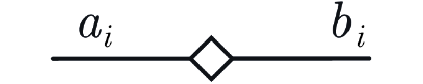
Symmetries disappear in 3 dimensions. From a graphical point of view, the move from ordered wires to named wires corresponds to moving from planar graphs to graphs in 3 dimensions. Instead of having a one dimensional line of inputs or outputs, wires are now sticking out of a plane [10]. As a benefit there are no wire-crossings, or, more technically, there are no symmetries to take care of. This simplifies the rewrite rules of calculi formulated in the named setting. For example, rules such as

[Uncaptioned image]

are not needed anymore. For more on this compare Figsย 3 andย 4.

Example: Simultaneous Substitutions. Substitutions $[a{\mapsto}b]$ can be composed sequentially and in parallel as in

$$[a{\mapsto}b]\hskip 1.03334pt;[b{\mapsto}c]=[a{\mapsto}c]\quad\quad\quad\quad[a{\mapsto}b]\uplus[c{\mapsto}d]=[a{\mapsto}b,c{\mapsto}d].$$

We call $\uplus$ the tensor, or the monoidal or vertical or parallel composition. Semantically, the simultaneous substitution on the right-hand side above, will correspond to the function $f:\{a,c\}\to\{b,d\}$ satisfying $f(a)=b$ and $f(c)=d$. Importantly, parallel composition of simultaneous substitutions is partial. For example, $[a{\mapsto}b]\uplus[a{\mapsto}c]$ is undefined, since there is no function $\{a\}\to\{b,c\}$ that maps $a$ simultaneously to both $b$ and $c$.

The advantages of a 2-dimensional calculus for simultaneous substitutions over a 1-dimensional calculus are the following. A calculus of substitutions is an algebraic representation, up to isomorphism, of the category $\mathsf{n}\mathbb{F}$ of finite subsets of $\mathcal{N}$. In a 1-dimensional calculus, operations $[a{\mapsto}b]$ have to be indexed by finite sets $S$

$$[a{\mapsto}b]_{S}:S\cup\{a\}\to S\cup\{b\}$$

for sets $S$ with $a,b\notin S.$ On the other hand, in a 2-dimensional calculus with an explicit operation $\uplus$ for set-union, indexing with subsets $S$ is unnecessary. Moreover, while the swapping

$$\{a,b\}\to\{a,b\}$$

in the 1-dimensional calculus needs an auxiliary name such as $c$ in $[a{\mapsto}c]_{\{b\}}\hskip 1.03334pt;[b{\mapsto}a]_{\{c\}}\hskip 1.03334pt;[c{\mapsto}a]_{\{b\}}$ it is represented in the 2-dimensional calculus directly by

$$[a{\mapsto}b]\uplus[b{\mapsto}a]$$

Finally, while it is possible to write down the equations and rewrite rules for the 1-dimensional calculus, it does not appear as particularly natural. In particular, only in the 2-dimensional calculus, will the swapping have a simple normal form such as $[a{\mapsto}b]\uplus[b{\mapsto}a]$ (unique up to commutativity of $\uplus$).

Overview. In order to account for partial tensors, Sectionย 3 develops the notion of a monoidal category internal in a symmetric monoidal category. Sectionย 4 is devoted to examples, while Sectionย 5 introduces the notion of a nominal prop and Sectionย 6 shows shat the categories of ordinary and of nominal props are equivalent.

2 Setting the Scene: String Diagrams and Nominal Sets

We review some of the necessary terminology but need to refer to the literature for details.

2.1 String Diagrams

The mathematical theory of string diagrams can be formalised via $\mathsf{PROP}$s as defined by MacLaneย [14]. There is also the weaker notion by Lackย [11], see Remark 2.9 of Zanasi [20] for a discussion.

A $\mathsf{PROP}$ (products and permutation category) is a symmetric strict monoidal category, with natural numbers as objects, where the monoidal tensor $\oplus$ is addition. Moreover, $\mathsf{PROP}$s, along with strict symmetric monoidal functors, that are identities on objects, form the category $\mathsf{PROP}$. A $\mathsf{PROP}$ contains all bijections between numbers as they can be be generated from the symmetry (twist) $1\oplus 1\to 1\oplus 1$ and from the parallel composition $\oplus$ and sequential composition ; (which we write in diagrammatic order).

$\mathsf{PROP}$s can be presented in algebraic form by operations and equations as symmetric monoidal theories ($\mathrm{SMT}$s) [20].

An $\mathrm{SMT}$ $(\Sigma,E)$ has a set $\Sigma$ of generators, where each generator $\gamma\in\Sigma$ is given an arity $m$ and co-arity $n$, usually written as $\gamma:m\to n$ and a set $E$ of equations, which are pairs of $\Sigma$-terms. $\Sigma$-terms can be obtained by composing generators in $\Sigma$ with the unit $\mathit{id}:1\to 1$ and symmetry $\sigma:2\to 2$, using either the parallel or sequential composition (see Figย 1). Equations $E$ are pairs of $\Sigma$-terms with the same arity and co-arity.

Refer to caption โ€ƒโ€ƒโ€ƒโ€ƒRefer to caption Refer to caption
$\displaystyle\frac{}{\gamma:m\to n\in\Sigma}$ $\displaystyle\frac{}{id:1\to 1}$ $\displaystyle\frac{}{\sigma:2\to 2}$
Refer to caption Refer to caption
$\displaystyle\frac{t:m\to n\quad\quad t^{\prime}:o\to p}{t\oplus t^{\prime}:m+o\to n+p}$ t:mโ†’ns:nโ†’ot;s:mโ†’o:๐‘กโ†’๐‘š๐‘›๐‘ :โ†’๐‘›๐‘œ:๐‘ก๐‘ โ†’๐‘š๐‘œ\displaystyle\frac{t:m\to n\quad\quad s:n\to o}{t\hskip 1.03334pt;s:m\to o}
Figure 1: SMT Terms

Given an $\mathrm{SMT}$, we can freely generate a $\mathsf{PROP}$, by taking $\Sigma$-terms as arrows, modulo the equations of Figย 2, together with the smallest congruence (with respect to the two compositions) of equations in $E$.

๐‘–๐‘‘m;t=t=t;๐‘–๐‘‘niโ€‹d0โŠ•t=t=tโŠ•iโ€‹d0(t;s);r=t;(s;r)(tโŠ•s)โŠ•r=tโŠ•(sโŠ•r)ฯƒ1,1;ฯƒ1,1=iโ€‹d2(s;t)โŠ•(u;v)=(sโŠ•u);(tโŠ•v)(tโŠ•iโ€‹dz);ฯƒn,z=ฯƒm,z;(iโ€‹dzโŠ•t)formulae-sequencesubscript๐‘–๐‘‘๐‘š๐‘ก๐‘ก๐‘กsubscript๐‘–๐‘‘๐‘›direct-sum๐‘–subscript๐‘‘0๐‘ก๐‘กdirect-sum๐‘ก๐‘–subscript๐‘‘0formulae-sequence๐‘ก๐‘ ๐‘Ÿ๐‘ก๐‘ ๐‘Ÿdirect-sumdirect-sum๐‘ก๐‘ ๐‘Ÿdirect-sum๐‘กdirect-sum๐‘ ๐‘Ÿsubscript๐œŽ11subscript๐œŽ11๐‘–subscript๐‘‘2direct-sum๐‘ ๐‘ก๐‘ข๐‘ฃdirect-sum๐‘ ๐‘ขdirect-sum๐‘ก๐‘ฃformulae-sequencedirect-sum๐‘ก๐‘–subscript๐‘‘๐‘งsubscript๐œŽ๐‘›๐‘งsubscript๐œŽ๐‘š๐‘งdirect-sum๐‘–subscript๐‘‘๐‘ง๐‘ก\begin{array}[]{cc}\mathit{id}_{m}\hskip 1.03334pt;t=t=t\hskip 1.03334pt;\mathit{id}_{n}{}&\qquad id_{0}\oplus t=t=t\oplus id_{0}\\[4.30554pt] (t\hskip 1.03334pt;s)\hskip 1.03334pt;r=t\hskip 1.03334pt;(s\hskip 1.03334pt;r){}&\qquad(t\oplus s)\oplus r=t\oplus(s\oplus r)\\[4.30554pt] \sigma_{1,1}\hskip 1.03334pt;\sigma_{1,1}=id_{2}{}&\qquad(s\hskip 1.03334pt;t)\oplus(u\hskip 1.03334pt;v)=(s\oplus u)\hskip 1.03334pt;(t\oplus v)\\[4.30554pt] \lx@intercol\hfil(t\oplus id_{z})\hskip 1.03334pt;\sigma_{n,z}=\sigma_{m,z}\hskip 1.03334pt;(id_{z}\oplus t)\hfil\lx@intercol\end{array}
Figure 2: Equations of symmetric monoidal categories

$\mathsf{PROP}$s admit a nice graphical presentation, wherein the sequential composition is modeled by horizontal composition of diagrams, and parallel/tensor composition is vertical stacking of diagrams (see Figย 1). We now present the $\mathrm{SMT}$s of bijections $\mathbb{B}$, injections $\mathbb{I}$, surjections $\mathbb{S}$, functions $\mathbb{F}$, partial functions $\mathbb{P}$, relations $\mathbb{R}$ and monotone maps $\mathbb{M}$.111The theory of monotone maps $\mathbb{M}$ does not include equations involving the symmetry $\sigma$ and is in fact presented by a so-called $\mathsf{PRO}$ rather than a $\mathsf{PROP}$. However, in this paper we will only be dealing with theories presented by $\mathsf{PROP}$s (the reason why this is the case is illustrated in the proof of Propositionย 6.3). The diagram in Figย 3 shows the generators and the equations that need to be added to the empty $\mathrm{SMT}$, to get a presentation of the given theory. To ease comparison with the corresponding nominal monoidal theories in Figย 4 later we also added on a striped background the equations for wire-crossings that are already implied by the naturality of symmetries, that is, the last equation of Figย 2. These are the equations that are part of the definition of a prop in the sense of MacLaneย [14] but need to be added explicitely to the props in the sense of Lackย [11].

Refer to caption
Figure 3: Symmetric monoidal theories

2.2 Nominal Sets

Let $\mathcal{N}$ be a countably infinite set of โ€˜namesโ€˜ or โ€˜atomsโ€˜. Let $\mathfrak{S}$ be the group of finite222A permutation is called finite if it is generated by finitely many transpositions. permutations $\mathcal{N}\to\mathcal{N}$. An element $x\in X$ of a group action $\mathfrak{S}\times X\to X$ is supported by $S\subseteq\mathcal{N}$ if $\pi\cdot x=x$ for all $\pi\in\mathfrak{S}$ such that $\pi$ restricted to $S$ is the identity. A group action $\mathfrak{S}\times X\to X$ such that all elements of $X$ have finite support is called a nominal set. We write $\mathsf{supp}(x)$ for the minimal support of $x$ and $\mathsf{Nom}$ for the category of nominal sets, which has as maps the equivariant functions, that is, those functions that respect the permutation action. Our main example is the category of simultaneous substitutions:

Example 2.1 (${\mathsf{n}\mathbb{F}}$).

We denote by ${\mathsf{n}\mathbb{F}}$ the category of finite subsets of $\mathcal{N}$ with all functions. While ${\mathsf{n}\mathbb{F}}$ is a category, it also carries additional nominal structure. In particular, both the set of objects and the set of arrows are nominal sets. with $\mathsf{supp}(A)=A$ and $\mathsf{supp}(f)=A\cup B$ for $f:A\to B$. The categories of injections, surjections, bijections, partial functions and relations are further examples along the same lines.

3 Internal monoidal categories

We introduce the notion of an internal monoidal category. Given a symmetric monoidal category $(\mathcal{V},I,\otimes)$ with finite limits, we are interested in categories $\mathbb{C}$, internal in $\mathcal{V}$, that carry a monoidal structure not of type $\mathbb{C}\times\mathbb{C}\to\mathbb{C}$ but of type $\mathbb{C}\otimes\mathbb{C}\to\mathbb{C}$. This will allow us to account for the partiality of $\uplus$ discussed in the introduction:

Example 3.1.
  • โ€ข

    The symmetric monoidal (closed) category $(\mathsf{Nom},1,\ast)$ of nominal sets with the separated product $\ast$ is defined as follows [16]. $1$ is the terminal object, ie, a singleton with empty support. The separated product of two nominal sets is defined as $A\ast B=\{(a,b)\in A\times B\mid\mathsf{supp}(a)\cap\mathsf{supp}(b)=\emptyset\}$.

  • โ€ข

    The category ${\mathsf{n}\mathbb{F}}$ (and its relatives) of Exampleย 2.1 is an internal monoidal category with monoidal operation given by $A\uplus B=A\cup B$ if $A$ and $B$ are disjoint.

$({\mathsf{n}\mathbb{F}},\emptyset,\uplus)$ as defined in the previous example is not a monoidal category, since $\uplus$, being partial, is not an operation of type ${\mathsf{n}\mathbb{F}}\times{\mathsf{n}\mathbb{F}}\to{\mathsf{n}\mathbb{F}}$ . The purpose of this section is to show that $({\mathsf{n}\mathbb{F}},\emptyset,\uplus)$ is an internal monoidal category in $(\mathsf{Nom},1,\ast)$ with $\uplus$ of type

$$\uplus:{\mathsf{n}\mathbb{F}}\ast{\mathsf{n}\mathbb{F}}\to{\mathsf{n}\mathbb{F}}.$$

To this end we need to extend $\ast:\mathsf{Nom}\times\mathsf{Nom}\to\mathsf{Nom}$ to

$$\ast:\mathsf{Cat}(\mathsf{Nom})\times\mathsf{Cat}(\mathsf{Nom})\to\mathsf{Cat}(\mathsf{Nom})$$

where we denote by $\mathsf{Cat}(\mathsf{Nom})$, the category of (small) internal categories in $\mathsf{Nom}$.

The necessary (and standard) notation from internal categories is reviewed in Appendix A.

Remark 3.2.

Let $\mathbb{C}$ be an internal category in a symmetric monoidal category $(\mathcal{V},I,\otimes)$ with finite limits. Since $\otimes$ need not preserve finite limits, we cannot expect that defining $(\mathbb{C}\otimes\mathbb{C})_{0}=\mathbb{C}_{0}\otimes\mathbb{C}_{0}$ and $(\mathbb{C}\otimes\mathbb{C})_{1}=\mathbb{C}_{1}\otimes\mathbb{C}_{1}$ results in $\mathbb{C}\otimes\mathbb{C}$ being an internal category.

Consequently, putting $(\mathbb{C}\otimes\mathbb{C})_{1}=\mathbb{C}_{1}\otimes\mathbb{C}_{1}$ does not extend $\otimes$ to an operation $\mathsf{Cat}(\mathcal{V})\times\mathsf{Cat}(\mathcal{V})\to\mathsf{Cat}(\mathcal{V})$. To show what goes wrong in a concrete instance is the purpose of the next example.

Example 3.3.

Define a binary operation ${\mathsf{n}\mathbb{F}}\ast{\mathsf{n}\mathbb{F}}$ as $({\mathsf{n}\mathbb{F}}\ast{\mathsf{n}\mathbb{F}})_{0}={\mathsf{n}\mathbb{F}}_{0}\ast{\mathsf{n}\mathbb{F}}_{0}$ and $({\mathsf{n}\mathbb{F}}\ast{\mathsf{n}\mathbb{F}})_{1}={\mathsf{n}\mathbb{F}}_{1}\ast{\mathsf{n}\mathbb{F}}_{1}$. Then ${\mathsf{n}\mathbb{F}}\ast{\mathsf{n}\mathbb{F}}$ cannot be equipped with the structure of an internal category. Indeed, assume for a contradiction that there was an appropriate pullback $({\mathsf{n}\mathbb{F}}\ast{\mathsf{n}\mathbb{F}})_{2}$ and arrow $\mathit{comp}$ such that the two diagrams commute:

$\textstyle{({\mathsf{n}\mathbb{F}}\ast{\mathsf{n}\mathbb{F}})_{2}\ \ignorespaces\ignorespaces\ignorespaces\ignorespaces\ignorespaces\ignorespaces\ignorespaces\ignorespaces\ignorespaces}$ $\scriptstyle{\ \mathit{comp}\ }$ $\scriptstyle{\pi_{1}}$ $\scriptstyle{\pi_{2}}$ $\textstyle{{\ \ {\mathsf{n}\mathbb{F}}_{1}\ast{\mathsf{n}\mathbb{F}}_{1}\ \ }\ignorespaces\ignorespaces\ignorespaces\ignorespaces}$ $\scriptstyle{\mathit{dom}}$ $\scriptstyle{\mathit{cod}}$ $\textstyle{{\mathsf{n}\mathbb{F}}_{1}\ast{\mathsf{n}\mathbb{F}}_{1}\ \ignorespaces\ignorespaces\ignorespaces\ignorespaces}$ $\scriptstyle{\ \mathit{dom}\ }$ $\scriptstyle{\mathit{cod}}$ $\textstyle{{\ \ {\mathsf{n}\mathbb{F}}_{0}\ast{\mathsf{n}\mathbb{F}}_{0}\ \ }}$

Let $\delta_{xy}:\{x\}\to\{y\}$ be the unique function in ${\mathsf{n}\mathbb{F}}$ of type $\{x\}\to\{y\}$. Then $((\delta_{ac},\delta_{bd}),(\delta_{cb},\delta_{da}))$, which can be depicted as

$\textstyle{\{a\}\ignorespaces\ignorespaces\ignorespaces\ignorespaces}$ $\scriptstyle{\delta_{ac}}$ $\textstyle{\{c\}\ignorespaces\ignorespaces\ignorespaces\ignorespaces}$ $\scriptstyle{\delta_{cb}}$ $\textstyle{\{b\}}$ $\textstyle{\{b\}\ignorespaces\ignorespaces\ignorespaces\ignorespaces}$ $\scriptstyle{\delta_{bd}}$ $\textstyle{\{d\}\ignorespaces\ignorespaces\ignorespaces\ignorespaces}$ $\scriptstyle{\delta_{da}}$ $\textstyle{\{a\}}$

is in the pullback $({\mathsf{n}\mathbb{F}}\ast{\mathsf{n}\mathbb{F}})_{2}$, but there is no $\mathit{comp}$ such that the two squares above commute, since $\mathit{comp}((\delta_{ac},\delta_{bd}),(\delta_{cb},\delta_{da}))$ would have to be $(\delta_{ab},\delta_{ba})$, which do not have disjoint support and therefore are not in ${\mathsf{n}\mathbb{F}}_{1}\ast{\mathsf{n}\mathbb{F}}_{1}$. โˆŽ

The solution to the problem consists in assuming that the given symmetric monoidal category with finite limits $(\mathcal{V},1,\otimes)$ is semi-cartesian (aka affine), that is, the unit $1$ is the terminal object. In such a category there are canonical

$$j:A\otimes B\to A\times B$$

and we can use them to define arrows $j_{1}:(\mathbb{C}\otimes\mathbb{C})_{1}\to\mathbb{C}_{1}\times\mathbb{C}_{1}$ that give us the right notion of tensor on arrows. From our example ${\mathsf{n}\mathbb{F}}$ above, we know that we want arrows $(f,g)$ to be in $(\mathbb{C}\otimes\mathbb{C})_{1}$ if $\mathit{dom}(f)\cap\mathit{dom}(g)=\emptyset$ and $\mathit{cod}(f)\cap\mathit{cod}(g)=\emptyset$. We now turn this observation into a category theoretic definition.

Let $\mathbb{C}$ and $\mathbb{D}$ be internal categories in $\mathcal{V}$. Our first task is to define $(\mathbb{C}\otimes\mathbb{D})_{1}$. This is accomplished by stipulating that $(\mathbb{C}\otimes\mathbb{D})_{1}$ is the limit in the diagram below

(โ„‚โŠ—๐”ป)1subscripttensor-productโ„‚๐”ป1{\definecolor[named]{.}{rgb}{0,1,1}\color[rgb]{0,1,1}\definecolor[named]{pgfstrokecolor}{rgb}{0,1,1}\pgfsys@color@cmyk@stroke{1}{0}{0}{0}\pgfsys@color@cmyk@fill{1}{0}{0}{0}(\mathbb{C}\otimes\mathbb{D})_{1}}โ„‚1ร—๐”ป1subscriptโ„‚1subscript๐”ป1{\definecolor[named]{.}{rgb}{0,0,0}\color[rgb]{0,0,0}\definecolor[named]{pgfstrokecolor}{rgb}{0,0,0}\pgfsys@color@gray@stroke{0}\pgfsys@color@gray@fill{0}\mathbb{C}_{1}\times\mathbb{D}_{1}}โ„‚0โŠ—๐”ป0tensor-productsubscriptโ„‚0subscript๐”ป0{\definecolor[named]{.}{rgb}{0,0,0}\color[rgb]{0,0,0}\definecolor[named]{pgfstrokecolor}{rgb}{0,0,0}\pgfsys@color@gray@stroke{0}\pgfsys@color@gray@fill{0}\mathbb{C}_{0}\otimes\mathbb{D}_{0}}โ„‚0ร—๐”ป0subscriptโ„‚0subscript๐”ป0{\definecolor[named]{.}{rgb}{0,0,0}\color[rgb]{0,0,0}\definecolor[named]{pgfstrokecolor}{rgb}{0,0,0}\pgfsys@color@gray@stroke{0}\pgfsys@color@gray@fill{0}\mathbb{C}_{0}\times\mathbb{D}_{0}}โ„‚0โŠ—๐”ป0tensor-productsubscriptโ„‚0subscript๐”ป0{\definecolor[named]{.}{rgb}{0,0,0}\color[rgb]{0,0,0}\definecolor[named]{pgfstrokecolor}{rgb}{0,0,0}\pgfsys@color@gray@stroke{0}\pgfsys@color@gray@fill{0}\mathbb{C}_{0}\otimes\mathbb{D}_{0}}โ„‚0ร—๐”ป0subscriptโ„‚0subscript๐”ป0{\definecolor[named]{.}{rgb}{0,0,0}\color[rgb]{0,0,0}\definecolor[named]{pgfstrokecolor}{rgb}{0,0,0}\pgfsys@color@gray@stroke{0}\pgfsys@color@gray@fill{0}\mathbb{C}_{0}\times\mathbb{D}_{0}}$j_{1}$ $\mathit{cod}_{(\mathbb{C}\otimes\mathbb{D})_{1}}$ $\mathit{dom}_{(\mathbb{C}\otimes\mathbb{D})_{1}}$ $j$ $j$ $\mathit{cod}_{\mathbb{C}_{1}}\times\mathit{cod}_{\mathbb{D}_{1}}$ $\mathit{dom}_{\mathbb{C}_{1}}\times\mathit{dom}_{\mathbb{D}_{1}}$

In the following we abbreviate the diagram above to

$\textstyle{(\mathbb{C}\otimes\mathbb{D})_{1}\ignorespaces\ignorespaces\ignorespaces\ignorespaces\ignorespaces\ignorespaces\ignorespaces\ignorespaces\ignorespaces\ignorespaces\ignorespaces\ignorespaces}$ $\scriptstyle{j_{1}}$ $\scriptstyle{\mathit{dom}}$ $\scriptstyle{\mathit{cod}}$ $\textstyle{\mathbb{C}_{1}\times\mathbb{D}_{1}\ignorespaces\ignorespaces\ignorespaces\ignorespaces\ignorespaces\ignorespaces\ignorespaces\ignorespaces}$ $\scriptstyle{\mathit{dom}\times\mathit{dom}}$ $\scriptstyle{\mathit{cod}\times\mathit{cod}}$ $\textstyle{(\mathbb{C}\otimes\mathbb{D})_{0}\ignorespaces\ignorespaces\ignorespaces\ignorespaces}$ $\scriptstyle{j}$ $\textstyle{\mathbb{C}_{0}\times\mathbb{D}_{0}}$ (1)

We are now in the position to extend the monoidal operation $\otimes:\mathcal{V}\times\mathcal{V}\to\mathcal{V}$ to a monoidal operation $\otimes:Cat(\mathcal{V})\times Cat(\mathcal{V})\to Cat(\mathcal{V})$.

Definition 3.4.

Let $(\mathcal{V},1,\otimes)$ be a monoidal category where the unit is the terminal object. The operation $\otimes:Cat(\mathcal{V})\times Cat(\mathcal{V})\to Cat(\mathcal{V})$ is defined as follows.

  • โ€ข

    (โ„‚โŠ—๐”ป)0subscripttensor-productโ„‚๐”ป0(\mathbb{C}\otimes\mathbb{D})_{0} and $(\mathbb{C}\otimes\mathbb{D})_{1}$ and $\mathit{cod},\mathit{dom}:(\mathbb{C}\otimes\mathbb{D})_{1}\to(\mathbb{C}\otimes\mathbb{D})_{0}$ as in the diagram above.

  • โ€ข

    i:(โ„‚โŠ—๐”ป)0โ†’(โ„‚โŠ—๐”ป)1:๐‘–โ†’subscripttensor-productโ„‚๐”ป0subscripttensor-productโ„‚๐”ป1i:(\mathbb{C}\otimes\mathbb{D})_{0}\to(\mathbb{C}\otimes\mathbb{D})_{1} is the arrow into the limit $(\mathbb{C}\otimes\mathbb{D})_{1}$ given by

    $\textstyle{(\mathbb{C}\otimes\mathbb{D})_{0}\ignorespaces\ignorespaces\ignorespaces\ignorespaces\ignorespaces\ignorespaces\ignorespaces\ignorespaces\ignorespaces\ignorespaces\ignorespaces\ignorespaces\ignorespaces\ignorespaces\ignorespaces\ignorespaces\ignorespaces\ignorespaces\ignorespaces\ignorespaces\ignorespaces\ignorespaces}$ $\scriptstyle{(i\times i)\circ j}$ $\scriptstyle{\ \mathit{id}\ }$ $\scriptstyle{\ \mathit{id}\ }$ $\scriptstyle{\ i\ }$ $\textstyle{(\mathbb{C}\otimes\mathbb{D})_{1}\ignorespaces\ignorespaces\ignorespaces\ignorespaces\ignorespaces\ignorespaces\ignorespaces\ignorespaces\ignorespaces\ignorespaces\ignorespaces\ignorespaces\ignorespaces}$ $\scriptstyle{\ j_{1}\ }$ $\scriptstyle{\mathit{cod}}$ $\scriptstyle{\mathit{dom}}$ $\textstyle{\mathbb{C}_{1}\times\mathbb{D}_{1}\ignorespaces\ignorespaces\ignorespaces\ignorespaces\ignorespaces\ignorespaces\ignorespaces\ignorespaces}$ $\scriptstyle{\mathit{cod}\times\mathit{cod}}$ $\scriptstyle{\mathit{dom}\times\mathit{dom}}$ $\textstyle{{\ \ (\mathbb{C}\otimes\mathbb{D})_{0}}\ignorespaces\ignorespaces\ignorespaces\ignorespaces}$ $\scriptstyle{j}$ $\textstyle{\mathbb{C}_{0}\times\mathbb{D}_{0}}$

    from which one reads off

    $$\mathit{dom}\circ i=\mathit{id}_{(\mathbb{C}\otimes\mathbb{D})_{0}}=\mathit{cod}\circ i$$
  • โ€ข

    (โ„‚โŠ—๐”ป)2subscripttensor-productโ„‚๐”ป2(\mathbb{C}\otimes\mathbb{D})_{2} is the pullback

    $\textstyle{(\mathbb{C}\otimes\mathbb{D})_{2}\ignorespaces\ignorespaces\ignorespaces\ignorespaces\ignorespaces\ignorespaces\ignorespaces\ignorespaces}$ $\scriptstyle{\pi_{1}}$ $\scriptstyle{\pi_{2}}$ $\textstyle{(\mathbb{C}\otimes\mathbb{D})_{1}\ignorespaces\ignorespaces\ignorespaces\ignorespaces}$ $\scriptstyle{\mathit{cod}}$ $\textstyle{(\mathbb{C}\otimes\mathbb{D})_{1}\ignorespaces\ignorespaces\ignorespaces\ignorespaces}$ $\scriptstyle{\mathit{dom}}$ $\textstyle{(\mathbb{C}\otimes\mathbb{D})_{0}}$

    Recalling the definition of $j_{1}$ from (1), there is also a corresponding $j_{2}:(\mathbb{C}\otimes\mathbb{D})_{2}\to\mathbb{C}_{2}\times\mathbb{D}_{2}$ due to the fact that the product of pullbacks is a pullback of products

    $\textstyle{(\mathbb{C}\otimes\mathbb{D})_{2}\ignorespaces\ignorespaces\ignorespaces\ignorespaces\ignorespaces\ignorespaces\ignorespaces\ignorespaces\ignorespaces\ignorespaces\ignorespaces\ignorespaces}$ $\scriptstyle{\pi_{1}}$ $\scriptstyle{\pi_{2}}$ $\scriptstyle{j_{2}}$ $\textstyle{\mathbb{C}_{2}\times\mathbb{D}_{2}\ignorespaces\ignorespaces\ignorespaces\ignorespaces\ignorespaces\ignorespaces\ignorespaces\ignorespaces}$ $\scriptstyle{\pi_{1}\times\pi_{1}}$ $\scriptstyle{\pi_{2}\times\pi_{2}}$ $\textstyle{(\mathbb{C}\otimes\mathbb{D})_{1}\ignorespaces\ignorespaces\ignorespaces\ignorespaces\ignorespaces\ignorespaces\ignorespaces\ignorespaces\ignorespaces\ignorespaces}$ $\scriptstyle{\mathit{cod}}$ $\scriptstyle{j_{1}}$ $\textstyle{(\mathbb{C}\otimes\mathbb{D})_{1}\ignorespaces\ignorespaces\ignorespaces\ignorespaces\ignorespaces\ignorespaces\ignorespaces\ignorespaces\ignorespaces\ignorespaces}$ $\scriptstyle{\mathit{dom}}$ $\scriptstyle{j_{1}}$ $\textstyle{\mathbb{C}_{1}\times\mathbb{D}_{1}\ignorespaces\ignorespaces\ignorespaces\ignorespaces}$ $\scriptstyle{\mathit{cod}\times\mathit{cod}}$ $\textstyle{\mathbb{C}_{1}\times\mathbb{D}_{1}\ignorespaces\ignorespaces\ignorespaces\ignorespaces}$ $\scriptstyle{\mathit{dom}\times\mathit{dom}}$ $\textstyle{(\mathbb{C}\otimes\mathbb{D})_{0}\ignorespaces\ignorespaces\ignorespaces\ignorespaces}$ $\scriptstyle{j}$ $\textstyle{\mathbb{C}_{0}\times\mathbb{D}_{0}}$ (2)

    Recall the definition of the limit $(\mathbb{C}\otimes\mathbb{D})_{1}$ from (1). Then $\mathit{comp}:(\mathbb{C}\otimes\mathbb{D})_{2}\to(\mathbb{C}\otimes\mathbb{D})_{1}$ is the arrow into $(\mathbb{C}\otimes\mathbb{D})_{1}$

    $\textstyle{(\mathbb{C}\otimes\mathbb{D})_{2}\ignorespaces\ignorespaces\ignorespaces\ignorespaces\ignorespaces\ignorespaces\ignorespaces\ignorespaces\ignorespaces\ignorespaces\ignorespaces\ignorespaces\ignorespaces\ignorespaces\ignorespaces\ignorespaces\ignorespaces\ignorespaces\ignorespaces\ignorespaces\ignorespaces\ignorespaces}$ $\scriptstyle{\ \ \ \ \ \ \ \ (\mathit{comp}\times\mathit{comp})\circ j_{2}}$ $\scriptstyle{\ \ \ \mathit{dom}\circ\pi_{1}\ }$ $\scriptstyle{\ \mathit{cod}\circ\pi_{2}\ }$ $\scriptstyle{\ \mathit{comp}\ }$ $\textstyle{(\mathbb{C}\otimes\mathbb{D})_{1}\ignorespaces\ignorespaces\ignorespaces\ignorespaces\ignorespaces\ignorespaces\ignorespaces\ignorespaces\ignorespaces\ignorespaces\ignorespaces\ignorespaces\ignorespaces}$ $\scriptstyle{\ j_{1}\ }$ $\scriptstyle{\mathit{cod}}$ $\scriptstyle{\mathit{dom}}$ $\textstyle{\mathbb{C}_{1}\times\mathbb{D}_{1}\ignorespaces\ignorespaces\ignorespaces\ignorespaces\ignorespaces\ignorespaces\ignorespaces\ignorespaces}$ $\scriptstyle{\mathit{cod}\times\mathit{cod}}$ $\scriptstyle{\mathit{dom}\times\mathit{dom}}$ $\textstyle{{\ \ (\mathbb{C}\otimes\mathbb{D})_{0}}\ignorespaces\ignorespaces\ignorespaces\ignorespaces}$ $\scriptstyle{j}$ $\textstyle{\mathbb{C}_{0}\times\mathbb{D}_{0}}$ (3)

    from which one reads off

    $$\mathit{dom}\circ\mathit{comp}=\mathit{dom}\circ\pi_{1}\ \quad\quad\ \mathit{cod}\circ\mathit{comp}=\mathit{cod}\circ\pi_{2}$$
  • โ€ข

    The equations $\mathit{comp}\circ\langle i\circ\mathit{dom},\mathit{id}_{(\mathbb{C}\otimes\mathbb{D})_{1}}\rangle=\mathit{id}_{(\mathbb{C}\otimes\mathbb{D})_{1}}=\mathit{comp}\circ\langle\mathit{id}_{(\mathbb{C}\otimes\mathbb{D})_{1}},i\circ\mathit{cod}\rangle$ are proved in Propositionย 3.6.

  • โ€ข

    The equation $\mathit{comp}\,\circ\,\mathit{compl}=\mathit{comp}\,\circ\,\mathit{compr}$ will be shown in Propositionย 3.7.

This ends the definition of $\mathbb{C}\otimes\mathbb{D}$ and the next few pages are devoted to showing that it is indeed an internal category. To prove the next propositions, we will need the following lemma, which can be skipped for now. It is a consequence of the general fact that the isomorphism $[\mathcal{I},\mathcal{C}](K_{A},D)\cong\mathcal{C}(A,\lim D)$ defining limits is natural in $A$ and $D$.

Lemma 3.5.

If in the diagram

$\textstyle{T\ignorespaces\ignorespaces\ignorespaces\ignorespaces\ignorespaces\ignorespaces\ignorespaces\ignorespaces\ignorespaces\ignorespaces\ignorespaces\ignorespaces\ignorespaces\ignorespaces\ignorespaces\ignorespaces\ignorespaces\ignorespaces}$ $\scriptstyle{k}$ $\scriptstyle{f_{1}}$ $\scriptstyle{f_{2}}$ $\scriptstyle{h}$ $\textstyle{P\ignorespaces\ignorespaces\ignorespaces\ignorespaces\ignorespaces\ignorespaces\ignorespaces\ignorespaces\ignorespaces\ignorespaces\ignorespaces\ignorespaces\ignorespaces\ignorespaces}$ $\scriptstyle{f^{\prime}_{1}}$ $\scriptstyle{f^{\prime}_{2}}$ $\scriptstyle{h^{\prime}}$ $\textstyle{(\mathbb{C}\otimes\mathbb{D})_{2}\ignorespaces\ignorespaces\ignorespaces\ignorespaces\ignorespaces\ignorespaces\ignorespaces\ignorespaces\ignorespaces\ignorespaces\ignorespaces\ignorespaces}$ $\scriptstyle{j_{2}}$ $\scriptstyle{\pi_{1}}$ $\scriptstyle{\pi_{2}}$ $\textstyle{\mathbb{C}_{2}\times\mathbb{D}_{2}\ignorespaces\ignorespaces\ignorespaces\ignorespaces\ignorespaces\ignorespaces\ignorespaces\ignorespaces}$ $\scriptstyle{\pi_{1}\times\pi_{1}}$ $\scriptstyle{\pi_{2}\times\pi_{2}}$ $\textstyle{(\mathbb{C}\otimes\mathbb{D})_{1}\ignorespaces\ignorespaces\ignorespaces\ignorespaces\ignorespaces\ignorespaces\ignorespaces\ignorespaces\ignorespaces\ignorespaces\ignorespaces\ignorespaces}$ $\scriptstyle{j_{1}}$ $\scriptstyle{\mathit{cod}}$ $\scriptstyle{\mathit{dom}}$ $\textstyle{\mathbb{C}_{1}\times\mathbb{D}_{1}\ignorespaces\ignorespaces\ignorespaces\ignorespaces\ignorespaces\ignorespaces\ignorespaces\ignorespaces}$ $\scriptstyle{\mathit{cod}\times\mathit{cod}}$ $\scriptstyle{\mathit{dom}\times\mathit{dom}}$ $\textstyle{{\ \ (\mathbb{C}\otimes\mathbb{D})_{0}}\ignorespaces\ignorespaces\ignorespaces\ignorespaces}$ $\scriptstyle{j}$ $\textstyle{\mathbb{C}_{0}\times\mathbb{D}_{0}}$

$f$ and $f^{\prime}$ are cones commuting with $j_{1}$ and $k$, that is, if

$\displaystyle\mathit{cod}\circ f_{1}$ $\displaystyle=\mathit{dom}\circ f_{2}$ (4)
$\displaystyle(\mathit{cod}\times\mathit{cod})\circ f^{\prime}_{1}$ $\displaystyle=(\mathit{dom}\times\mathit{dom})\circ f^{\prime}_{2}$ (5)
$\displaystyle j_{1}\circ f_{i}$ $\displaystyle=f^{\prime}_{i}\circ k$ (6)

and $h,h^{\prime}$ are the respective unique arrows into the pullbacks, then also

$$h^{\prime}\circ k=j_{2}\circ h$$

holds.

Using the lemma, the next two propositions have reasonably straight forward proofs.

Proposition 3.6.

$\mathit{comp}\circ\langle i\circ\mathit{dom},\mathit{id}_{(\mathbb{C}\otimes\mathbb{D})_{1}}\rangle=\mathit{id}_{(\mathbb{C}\otimes\mathbb{D})_{1}}=\mathit{comp}\circ\langle\mathit{id}_{(\mathbb{C}\otimes\mathbb{D})_{1}},i\circ\mathit{cod}\rangle$.

Proposition 3.7.

$\mathit{comp}\circ\mathit{compl}=\mathit{comp}\circ\mathit{compr}$

This finishes the verification that $\mathbb{C}\otimes\mathbb{D}$ is an internal category. We next show that $1$ carries the structure of an internal monoidal category.

Proposition 3.8.

Let $(\mathcal{V},1,\otimes)$ be a monoidal category where the unit is the terminal object. $1$ carries the structure of an internal monoidal category $\mathbb{1}$ which is the neutral element wrt to the internal tensor $\otimes:Cat(\mathcal{V})\times Cat(\mathcal{V})\to Cat(\mathcal{V})$ of Definitionย 3.4.

The next step is to show that the $\otimes:Cat(\mathcal{V})\times Cat(\mathcal{V})\to Cat(\mathcal{V})$ of Definitionย 3.4 can be extended to a functor.

Proposition 3.9.

Let $(\mathcal{V},1,\otimes)$ be a monoidal category with finite limits where the unit is the terminal object. The internal tensor $\otimes:Cat(\mathcal{V})\times Cat(\mathcal{V})\to Cat(\mathcal{V})$ of Definitionย 3.4 is functorial.

The main result of the section is

Theorem 3.10.

Let $(\mathcal{V},1,\otimes)$ be a (symmetric) monoidal category with finite limits where the unit is the terminal object and $\otimes:Cat(\mathcal{V})\times Cat(\mathcal{V})\to Cat(\mathcal{V})$ the internal tensor of Definitionย 3.4. Then $(Cat(\mathcal{V}),\mathbb{1},\otimes)$ is a (symmetric) monoidal category.

Finally, internal strict monoidal categories organise themselves in a (2-)category.

Definition 3.11.

We denote by $\mathsf{Mon}(\mathsf{Cat}(\mathcal{V}),\mathbb{1},\otimes))$, or briefly, $\mathsf{Mon}(\mathsf{Cat}(\mathcal{V}))$, the category of monoids in $(\mathsf{Cat}(\mathcal{V}),\mathbb{1},\otimes))$.

Theorem 3.12.

$\mathsf{Mon}(\mathsf{Cat}(\mathcal{V}),\mathbb{1},\otimes))$ is a 2-category.

4 Examples

Before we give a formal definition of nominal $\mathsf{PROP}$s and nominal monoidal theories (NMTs) in the next section, we present as examples those NMTs that correspond to the SMTs of Figย 3. The nominal monoidal theories of Figย 4 should be immediately recognizable, indeed the significant differences are that wires now carry labels and there is a new generator [Uncaptioned image] which allows us to change the label of a wire.

Refer to caption

bijections $\mathsf{n}\mathbb{B}$, injections $\mathsf{n}\mathbb{I}$, surjections $\mathsf{n}\mathbb{S}$, functions $\mathsf{n}\mathbb{F}$, partial functions $\mathsf{n}\mathbb{P}$ and relations $\mathsf{n}\mathbb{R}$

Figure 4: Nominal monoidal theories
Theorem 4.1.

The calculi of Fig 4 are complete.

The proof of the theorem shows that the categories presented by Fig 4 are isomorphic to the categories of finite sets with the respective maps. These proofs seem easier for NMTs than the corresponding proofs for SMTs (see eg Lafontย [12]) because NMTs have no wire crossings. For example, in the case of bijections, it is immediate that every nominal diagram rewrites to a normal form, which is a parallel composition of diagrams of the form [Uncaptioned image]. Completeness then follows, as usual, from the possibility to rewrite every diagram into normal form. The other cases are only slightly more complicated.

5 Nominal monoidal theories and nominal PROPs

In this section, we introduce nominal $\mathsf{PROP}$s as internal monoidal categories in nominal sets. We first spell out the details of what that means in elementary terms and then discuss the notion of diagrammatic alpha-equivalence.

5.1 Nominal monoidal theories

A nominal monoidal theory $(\Sigma,E)$ is given by a nominal set $\Sigma$ of generators and a nominal set $E$ of equations. A generator $\gamma:A\to B$ has finite sets $A,B$ of names as types and $\Sigma$ is closed under permutations $\pi\cdot\gamma:\pi\cdot A\to\pi\cdot B$. The set of terms is given by closing under the operations of Figย 5, which should be compared with Figย 1.

$$\displaystyle\frac{}{\gamma:A\to B\in\Sigma}\qquad\qquad\frac{}{id_{a}:\{a\}\to\{a\}}\qquad\qquad\frac{}{\delta_{ab}:\{a\}\to\{b\}}$$
t:Aโ†’Btโ€ฒ:Aโ€ฒโ†’Bโ€ฒtโŠŽtโ€ฒ:AโŠŽAโ€ฒโ†’BโŠŽBโ€ฒt:Aโ†’Bs:Bโ†’Ct;s:Aโ†’C:๐‘กโ†’๐ด๐ตsuperscript๐‘กโ€ฒ:โ†’superscript๐ดโ€ฒsuperscript๐ตโ€ฒ:โŠŽ๐‘กsuperscript๐‘กโ€ฒโ†’โŠŽ๐ดsuperscript๐ดโ€ฒโŠŽ๐ตsuperscript๐ตโ€ฒ:๐‘กโ†’๐ด๐ต๐‘ :โ†’๐ต๐ถ:๐‘ก๐‘ โ†’๐ด๐ถ\displaystyle\frac{t:A\to B\quad\quad t^{\prime}:A^{\prime}\to B^{\prime}}{t\uplus t^{\prime}:A\uplus A^{\prime}\to B\uplus B^{\prime}}\qquad\qquad\frac{t:A\to B\quad\quad s:B\to C}{t\hskip 1.03334pt;s:A\to C}
$$\displaystyle\frac{t:A\to B}{(a\ b)\,t:(a\ b)\cdot A\to(a\ b)\cdot B}$$
Figure 5: NMT Terms

Every NMT freely generates a monoidal category internal in nominal sets by quotienting the generated terms by the equations $E$ as well as by equations describing that terms form a monoidal category and a nominal set. The equations of an internal monoidal category are given in Figย 6. The main difference with the equations in Figย 2 is that the interchange law for $\uplus$ is required to hold only if both sides are defined and that the two laws involving symmetries are replaced by the commutativity of $\uplus$.

๐‘–๐‘‘A;t=t=t;๐‘–๐‘‘Biโ€‹dโˆ…โŠŽt=t=tโŠŽiโ€‹dโˆ…(t;s);r=t;(s;r)(tโŠŽs)โŠŽr=tโŠŽ(sโŠŽr)tโŠŽs=sโŠŽt(s;t)โŠŽ(u;v)=(sโŠŽu);(tโŠŽv)formulae-sequencesubscript๐‘–๐‘‘๐ด๐‘ก๐‘ก๐‘กsubscript๐‘–๐‘‘๐ตโŠŽ๐‘–subscript๐‘‘๐‘ก๐‘กโŠŽ๐‘ก๐‘–subscript๐‘‘formulae-sequence๐‘ก๐‘ ๐‘Ÿ๐‘ก๐‘ ๐‘ŸโŠŽโŠŽ๐‘ก๐‘ ๐‘ŸโŠŽ๐‘กโŠŽ๐‘ ๐‘ŸโŠŽ๐‘ก๐‘ โŠŽ๐‘ ๐‘กโŠŽ๐‘ ๐‘ก๐‘ข๐‘ฃโŠŽ๐‘ ๐‘ขโŠŽ๐‘ก๐‘ฃ\begin{array}[]{cc}\mathit{id}_{A}\hskip 1.03334pt;t=t=t\hskip 1.03334pt;\mathit{id}_{B}{}&\qquad id_{\varnothing}\uplus t=t=t\uplus id_{\varnothing}\\[4.30554pt] (t\hskip 1.03334pt;s)\hskip 1.03334pt;r=t\hskip 1.03334pt;(s\hskip 1.03334pt;r){}&\qquad(t\uplus s)\uplus r=t\uplus(s\uplus r)\\[4.30554pt] t\uplus s=s\uplus t{}&\qquad(s\hskip 1.03334pt;t)\uplus(u\hskip 1.03334pt;v)=(s\uplus u)\hskip 1.03334pt;(t\uplus v)\end{array}
Figure 6: NMT Equations of internal monoidal categories

For terms to form a nominal set, we need the usual equations between permutations (not listed here) to hold, as well as the equations of Figย 7 that specify how permutations act on terms.

$$\displaystyle(a\ b)id_{x}=id_{(a\ b)\cdot x}\qquad\qquad(a\ b)\delta_{xy}=\delta_{(a\ b)\cdot x\ (a\ b)\cdot y}\qquad\qquad(a\ b)\gamma=(a\ b)\cdot\gamma$$
$$\displaystyle(a\ b)(x\uplus y)=(a\ b)x\uplus(a\ b)y\qquad\qquad(a\ b)(x\hskip 1.03334pt;y)=(a\ b)x\hskip 1.03334pt;(a\ b)y\qquad\qquad\delta_{ab}\hskip 1.03334pt;\delta_{bc}=\delta_{ac}$$
Refer to caption Refer to caption Refer to caption
$\frac{\gamma:A\to B\uplus\{b\}\qquad b,x\notin A}{\gamma\,{;}\,(\mathit{id}_{B}\uplus\delta_{bx})=(b\ x)\gamma}$ $\frac{\gamma:\{a\}\uplus A\to B\qquad a,x\notin B}{(\delta_{xa}\uplus\mathit{id}_{A})\,{;}\,\gamma=(x\ a)\gamma}$ $\frac{\gamma:A\uplus\{c\}\to B\uplus\{c\}}{\gamma\,{;}\,(\mathit{id}_{B}\uplus\delta_{cx})=(\mathit{id}_{A}\uplus\delta_{cx})\hskip 0.72334pt;(c\ x)\gamma}$
Figure 7: NMT Equations of nominal sets

These are routine, with the exception of the last three, specifying the interaction of renamings $\delta$ with renamings and generators $\gamma\in\Sigma$, which we also depict in diagrammatic form. Instances of these rules can be seen in Figย 4, where they are distinguished by a striped background.

5.2 Diagrammatic alpha-equivalence

The equations of Figย 7 introduce a notion of diagrammatic alpha-equivalence, which allows us to rename โ€˜internalโ€™ names and to contract renamings.

Definition 5.1.

Two terms of a nominal monoidal theory are alpha-equivalent if their equality follows from the equations in Figย 7.

Notation: Every permutation $\pi$ of names gives rise to bijective functions $\pi_{A}:A\to\pi[A]=\{\pi(a)\mid a\in A\}=\pi\cdot A$. Any such $\pi_{A}$, as well as the inverse $\pi_{A}^{-1}$, are parallel compositions of $\delta_{ab}$ for suitable $a,b\in\mathcal{N}$. In fact, we have $\pi_{A}=\biguplus_{a\in A}\delta_{a\pi(a)}$. We may therefore use the $\pi_{A}$ as abbreviations in terms.

Proposition 5.2.

Let $t:A\to B$ be a term of a nominal monoidal theory. The equations in Figย 7 entail that $\pi\cdot t=(\pi_{A})^{-1}\hskip 1.03334pt;t\hskip 1.03334pt;\pi_{B}$.

$\textstyle{A\ignorespaces\ignorespaces\ignorespaces\ignorespaces\ignorespaces\ignorespaces\ignorespaces\ignorespaces}$ $\scriptstyle{t}$ $\scriptstyle{\pi_{A}}$ $\textstyle{B\ignorespaces\ignorespaces\ignorespaces\ignorespaces}$ $\scriptstyle{\pi_{B}}$ $\textstyle{\pi[A]\ignorespaces\ignorespaces\ignorespaces\ignorespaces}$ $\scriptstyle{\pi\cdot t}$ $\textstyle{\pi[B]}$
Corollary 5.3.

Let $t:A\uplus\{c\}\to B\uplus\{c\}$ be a term of a nominal monoidal theory and $d{\#}t$. Then $t=(\delta_{cd}\uplus\mathit{id}_{A})\hskip 1.03334pt;(c\ d)\cdot t\hskip 1.03334pt;(\delta_{dc}\uplus\mathit{id}_{B})$.

Corollary 5.4.

Let $t:A\to B$ be a term of a nominal monoidal theory. Modulo the equations of Figย 7, the support of $t$ is $A\cup B$.

The last corollary shows that internal names are bound by sequential composition. Indeed, in a composition Aโ†’tCโ†’sBsuperscriptโ†’๐‘ก๐ด๐ถsuperscriptโ†’๐‘ ๐ตA\stackrel{{\scriptstyle t}}{{\to}}C\stackrel{{\scriptstyle s}}{{\to}}B, the names in $C\setminus(A\cup B)$ do not appear in the support of t;s๐‘ก๐‘ t\hskip 1.03334pt;s.

5.3 Nominal PROPs

From the point of view of Sectionย 3, a nominal $\mathsf{PROP}$ is an internal strict monoidal category in $(\mathsf{Nom},1,\ast)$ that has finite sets of names as objects and at least all bijections as arrows. We spell this out in detail.

Remark 5.5.

A nominal $\mathsf{PROP}$ $\mathbb{C}$ is a small category, with a set $\mathbb{C}_{0}$ of โ€˜objectsโ€™ and a set $\mathbb{C}_{1}$ of โ€˜arrowsโ€™, defined as follows. We write ; for the โ€˜sequentialโ€™ composition (in the diagrammatic order) and $\uplus$ for the โ€˜parallelโ€™ or โ€˜monoidalโ€™ composition.

  • โ€ข

    โ„‚0subscriptโ„‚0\mathbb{C}_{0} is the set of finite subsets of $\mathcal{N}$. The permutation action is given by $\pi\cdot A=\pi[A]=\{\pi(a)\mid a\in A\}$.

  • โ€ข

    โ„‚1subscriptโ„‚1\mathbb{C}_{1} contains all bijections (โ€˜renamingsโ€™) $\pi_{A}:A\to\pi\cdot A$ for all finite permutations $\pi:\mathcal{N}\to\mathcal{N}$ and is closed under the operation mapping an arrow $f:A\to B$ to $\pi\cdot f:\pi\cdot A\to\pi\cdot B$ defined as $\pi\cdot f=(\pi_{A})^{-1}{;}f{;}\pi_{B}$.

  • โ€ข

    AโŠŽBโŠŽ๐ด๐ตA\uplus B is the union of $A$ and $B$ and defined whenever $A$ and $B$ are disjoint. This makes $(\mathbb{C}_{0},\emptyset,\uplus)$ a commutative partial monoid. On arrows, we require $(\mathbb{C}_{1},\emptyset,\uplus)$ to be a commutative partial monoid, with $f\uplus g$ defined whenever $\mathit{dom}f\cap\mathit{dom}g=\emptyset$ and $\mathit{cod}f\cap\mathit{cod}g=\emptyset$.

From this definition on can deduce the following.

Remark 5.6.
  • โ€ข

    A nominal prop has a nominal set of objects and a nominal set of arrows.

  • โ€ข

    The support of an object $A$ is $A$ and the support of an arrow $f:A\to B$ is $A\cup B$. In particular, $\mathsf{supp}(f{;}g)=\mathit{dom}(f)\cup\mathit{cod}(g)$. In other words, nominal props have diagrammatic alpha equivalence.

  • โ€ข

    There is a category $\mathsf{n}\mathsf{PROP}$ that consists of nominal props together with functors that are the identity on objects and strict monoidal and equivariant.

  • โ€ข

    Every NMT presents a $\mathsf{n}\mathsf{PROP}$. Conversely, every $\mathsf{n}\mathsf{PROP}$ is presented by at least one NMT given by all terms as generators and all equations as equations.

6 Equivalence of nominal and ordinary string diagrams

We show that the categories $\mathsf{n}\mathsf{PROP}$ and $\mathsf{PROP}$ are equivalent.

To define translations between ordinary and nominal monoidal theories we introduce some auxiliary notation. We denote lists that contain each letter at most once by bold letters. If $\boldsymbol{a}=[a_{1},\ldots a_{n}]$ is a list, then $\underline{\boldsymbol{a}}=\{a_{1},\ldots a_{n}\}$. Given lists $\boldsymbol{a}$ and $\boldsymbol{a}^{\prime}$ with $\underline{\boldsymbol{a}}=\underline{\boldsymbol{a}^{\prime}}$ we abbreviate bijections in $\mathsf{PROP}$ (also called symmetries) mapping $i\mapsto a_{i}=a^{\prime}_{j}\mapsto j$ as $\langle\boldsymbol{a}|\boldsymbol{a}^{\prime}\rangle$. Given lists $\boldsymbol{a}$ and $\boldsymbol{b}$ of the same length we write $[\boldsymbol{a}|\boldsymbol{b}]=\biguplus\delta_{a_{i}b_{i}}$ for the bijection $a_{i}\mapsto b_{i}$ in an $\mathsf{n}\mathsf{PROP}$.

Proposition 6.1.

For any $\mathsf{PROP}$ $\mathcal{S}$, there is an $\mathsf{n}\mathsf{PROP}$

$$\mathit{NOM}(\mathcal{S})$$

that has for all arrows $f:\underline{n}\to\underline{m}$ of $\mathcal{S}$, and for all lists $\boldsymbol{a}=[a_{1},\ldots a_{n}]$ and $\boldsymbol{b}=[b_{1},\ldots b_{m}]$ arrows $[\boldsymbol{a}\rangle f\langle\boldsymbol{b}]$. These arrows are subject to equations

$\displaystyle[\boldsymbol{a}\rangle f\hskip 1.03334pt;g\langle\boldsymbol{c}]$ $\displaystyle=[\boldsymbol{a}\rangle f\langle\boldsymbol{b}]\hskip 1.03334pt;[\boldsymbol{b}\rangle g\langle\boldsymbol{c}]$
$\displaystyle[\boldsymbol{a}+\boldsymbol{c}\rangle f\oplus g\langle\boldsymbol{b}+\boldsymbol{d}]$ $\displaystyle=[\boldsymbol{a}\rangle f\langle\boldsymbol{b}]\uplus[\boldsymbol{c}\rangle g\langle\boldsymbol{d}]$
$\displaystyle[\boldsymbol{a}\rangle\mathit{id}\langle\boldsymbol{b}]$ $\displaystyle=[\boldsymbol{a}|\boldsymbol{b}]$
$\displaystyle[\boldsymbol{a}\rangle\,\langle\boldsymbol{b}|\boldsymbol{b}^{\prime}\rangle\hskip 1.03334pt;f\,\langle\boldsymbol{c}]\,$ $\displaystyle=[\boldsymbol{a}|\boldsymbol{b}]\hskip 1.03334pt;[\boldsymbol{b}^{\prime}\rangle f\langle\boldsymbol{c}]$
$\displaystyle[\boldsymbol{a}\rangle\,f\hskip 1.03334pt;\langle\boldsymbol{b}|\boldsymbol{b}^{\prime}\rangle\,\langle\boldsymbol{c}]\,$ $\displaystyle=[\boldsymbol{a}\rangle f\langle\boldsymbol{b}]\hskip 1.03334pt;[\boldsymbol{b}^{\prime}|\boldsymbol{c}]$
Proof 6.2.

To show that $\mathit{NOM}(\mathcal{S})$ is well-defined, we need to check that the equations of $\mathcal{S}$ are respected. We only have space here for the most interesting case which is the naturality of symmetries given by the last equation in Figย 2. We write $\boldsymbol{a}^{m}$ for a list of $a$โ€™s of length $m$.

$\displaystyle[\boldsymbol{a}^{m}+\boldsymbol{a}^{z}\rangle\,(t\oplus id_{z})\hskip 1.03334pt;\sigma_{n,z}\,\langle\boldsymbol{b}^{z}+\boldsymbol{b}^{n}]$ $\displaystyle=([\boldsymbol{a}^{m}\rangle\,t\,\langle\boldsymbol{x}^{n}]\uplus[\boldsymbol{a}^{z}\rangle\,id_{z}\,\langle\boldsymbol{x}^{z}])\hskip 1.03334pt;[\boldsymbol{x}^{n}+\boldsymbol{x}^{z}\rangle\,\sigma_{n,z}\,\langle\boldsymbol{b}^{z}+\boldsymbol{b}^{n}]$
$\displaystyle=([\boldsymbol{a}^{z}\rangle\,id_{z}\,\langle\boldsymbol{x}^{z}]\uplus[\boldsymbol{a}^{m}\rangle\,t\,\langle\boldsymbol{x}^{n}])\hskip 1.03334pt;[\boldsymbol{x}^{n}+\boldsymbol{x}^{z}\rangle\,\sigma_{n,z}\,\langle\boldsymbol{b}^{z}+\boldsymbol{b}^{n}]$
$\displaystyle=[\boldsymbol{a}^{z}+\boldsymbol{a}^{m}\rangle\,id_{z}\oplus t\,\langle\boldsymbol{x}^{z}+\boldsymbol{x}^{n}]\hskip 1.03334pt;[\boldsymbol{x}^{n}+\boldsymbol{x}^{z}\rangle\,\sigma_{n,z}\,\langle\boldsymbol{b}^{z}+\boldsymbol{b}^{n}]$
$\displaystyle=[\boldsymbol{a}^{z}+\boldsymbol{a}^{m}\rangle\,id_{z}\oplus t\,\langle\boldsymbol{x}^{z}+\boldsymbol{x}^{n}]\hskip 1.03334pt;[\boldsymbol{x}^{n}+\boldsymbol{x}^{z}\rangle\,\langle\boldsymbol{x}^{n}+\boldsymbol{x}^{z}|\boldsymbol{x}^{z}+\boldsymbol{x}^{n}\rangle\,\langle\boldsymbol{b}^{z}+\boldsymbol{b}^{n}]$
$\displaystyle=[\boldsymbol{a}^{z}+\boldsymbol{a}^{m}\rangle\,id_{z}\oplus t\,\langle\boldsymbol{x}^{z}+\boldsymbol{x}^{n}]\hskip 1.03334pt;[\boldsymbol{x}^{n}+\boldsymbol{x}^{z}|\boldsymbol{x}^{n}+\boldsymbol{x}^{z}]\hskip 1.03334pt;[\boldsymbol{x}^{z}+\boldsymbol{x}^{n}|\boldsymbol{b}^{z}+\boldsymbol{b}^{n}]$
$\displaystyle=[\boldsymbol{a}^{z}+\boldsymbol{a}^{m}\rangle\,id_{z}\oplus t\,\langle\boldsymbol{x}^{z}+\boldsymbol{x}^{n}]\hskip 1.03334pt;[\boldsymbol{x}^{z}+\boldsymbol{x}^{n}|\boldsymbol{b}^{z}+\boldsymbol{b}^{n}]$
$\displaystyle=[\boldsymbol{a}^{z}+\boldsymbol{a}^{m}\rangle\,id_{z}\oplus t\,\langle\boldsymbol{b}^{z}+\boldsymbol{b}^{n}]$
$\displaystyle=[\boldsymbol{a}^{m}+\boldsymbol{a}^{z}|\boldsymbol{a}^{m}+\boldsymbol{a}^{z}]\ \hskip 1.03334pt;\ [\boldsymbol{a}^{z}+\boldsymbol{a}^{m}\rangle\,id_{z}\oplus t\,\langle\boldsymbol{b}^{z}+\boldsymbol{b}^{n}]$
$\displaystyle=[\boldsymbol{a}^{m}+\boldsymbol{a}^{z}\rangle\,\langle\boldsymbol{a}^{m}+\boldsymbol{a}^{z}|\boldsymbol{a}^{z}+\boldsymbol{a}^{m}\rangle\hskip 1.03334pt;(id_{z}\oplus t)\,\langle\boldsymbol{b}^{z}+\boldsymbol{b}^{n}]$
$\displaystyle=[\boldsymbol{a}^{m}+\boldsymbol{a}^{z}\rangle\,\sigma_{m,z}\hskip 1.03334pt;(id_{z}\oplus t)\,\langle\boldsymbol{b}^{z}+\boldsymbol{b}^{n}]\ \hskip 90.00014pt$

Note how commutativity of $\uplus$ is used to show that naturality of symmetries is respected.

Proposition 6.3.

For any $\mathsf{n}\mathsf{PROP}$ $\mathcal{T}$ there is a $\mathsf{PROP}$

$$\mathit{ORD}(\mathcal{T})$$

that has for all arrows $f:A\to B$ of $\mathcal{T}$, and for all lists $\boldsymbol{a}=[a_{1},\ldots a_{n}]$ and $\boldsymbol{b}=[b_{1},\ldots b_{m}]$ arrows $\langle\boldsymbol{a}]f[\boldsymbol{b}\rangle$. These arrows are subject to equations

$\displaystyle\langle\boldsymbol{a}]\,f\hskip 1.03334pt;g\,[\boldsymbol{c}\rangle$ $\displaystyle=\langle\boldsymbol{a}]\,f\,[\boldsymbol{b}\rangle\hskip 1.03334pt;\langle\boldsymbol{b}]\,g\,[\boldsymbol{c}\rangle$
$\displaystyle\langle\boldsymbol{a}_{f}+\boldsymbol{a}_{g}]\,f\uplus g\,[\boldsymbol{b}_{f}+\boldsymbol{b}_{g}\rangle$ $\displaystyle=\langle\boldsymbol{a}_{f}]\,f\,[\boldsymbol{b}_{f}\rangle\oplus\langle\boldsymbol{a}_{g}]\,g\,[\boldsymbol{b}_{g}\rangle$
$\displaystyle\langle\boldsymbol{a}]\,\mathit{id}\,[\boldsymbol{a}\rangle$ $\displaystyle=\mathit{id}$
$\displaystyle\langle\boldsymbol{a}]\,[\boldsymbol{a}^{\prime}|\boldsymbol{b}]\hskip 1.03334pt;f\,[\boldsymbol{c}\rangle$ $\displaystyle=\langle\boldsymbol{a}|\boldsymbol{a}^{\prime}\rangle\hskip 1.03334pt;\langle\boldsymbol{b}]\,f\,[\boldsymbol{c}\rangle$
$\displaystyle\langle\boldsymbol{a}]\,f\hskip 1.03334pt;[\boldsymbol{b}|\boldsymbol{c}]\,[\boldsymbol{c}^{\prime}\rangle$ $\displaystyle=\langle\boldsymbol{a}]\,f\,[\boldsymbol{b}\rangle\hskip 1.03334pt;\langle\boldsymbol{c}|\boldsymbol{c}^{\prime}\rangle$
Proof 6.4.

To show that $\mathit{ORD}$ is well defined we need to show that the equations of an NMT are respected. The most interesting case here is the commutativity of $\uplus$ since the $\oplus$ of SMTs is not commutative.

$\displaystyle\langle\boldsymbol{a}_{t}+\boldsymbol{a}_{s}]\,t\uplus s\,[\boldsymbol{b}_{t}+\boldsymbol{b}_{s}\rangle$ $\displaystyle=\langle\boldsymbol{a}_{t}]\,t\,[\boldsymbol{b}_{t}\rangle\oplus\langle\boldsymbol{a}_{s}]\,s\,[\boldsymbol{b}_{s}\rangle$
$\displaystyle=(\langle\boldsymbol{a}_{t}]\,t\,[\boldsymbol{b}_{t}\rangle\ \hskip 1.03334pt;\ id_{|\boldsymbol{b}_{t}|})\oplus(id_{|\boldsymbol{a}_{s}|}\ \hskip 1.03334pt;\,\langle\boldsymbol{a}_{s}]\,s\,[\boldsymbol{b}_{s}\rangle)$
$\displaystyle=(\langle\boldsymbol{a}_{t}]\,t\,[\boldsymbol{b}_{t}\rangle\oplus id_{|\boldsymbol{a}_{s}|})\ \hskip 1.03334pt;\,(id_{|\boldsymbol{b}_{t}|}\oplus\langle\boldsymbol{a}_{s}]\,s\,[\boldsymbol{b}_{s}\rangle)$
$\displaystyle=(\langle\boldsymbol{a}_{t}]\,t\,[\boldsymbol{b}_{t}\rangle\oplus id_{|\boldsymbol{a}_{s}|})\,\hskip 1.03334pt;\,\sigma_{|\boldsymbol{b}_{t}|,|\boldsymbol{a}_{s}|}\,\hskip 1.03334pt;\,\sigma_{|\boldsymbol{a}_{s}|,|\boldsymbol{b}_{t}|}\,\hskip 1.03334pt;\,(id_{|\boldsymbol{b}_{t}|}\oplus\langle\boldsymbol{a}_{s}]\,s\,[\boldsymbol{b}_{s}\rangle)$
$\displaystyle=\sigma_{|\boldsymbol{a}_{t}|,|\boldsymbol{a}_{s}|}\,\hskip 1.03334pt;\,(id_{|\boldsymbol{a}_{s}|}\oplus\langle\boldsymbol{a}_{t}]\,t\,[\boldsymbol{b}_{t}\rangle)\,\hskip 1.03334pt;\,\sigma_{|\boldsymbol{a}_{s}|,|\boldsymbol{b}_{t}|}\,\hskip 1.03334pt;\,(id_{|\boldsymbol{b}_{t}|}\oplus\langle\boldsymbol{a}_{s}]\,s\,[\boldsymbol{b}_{s}\rangle)$
$\displaystyle=\sigma_{|\boldsymbol{a}_{t}|,|\boldsymbol{a}_{s}|}\,\hskip 1.03334pt;\,(id_{|\boldsymbol{a}_{s}|}\oplus\langle\boldsymbol{a}_{t}]\,t\,[\boldsymbol{b}_{t}\rangle)\ \hskip 1.03334pt;\ (\langle\boldsymbol{a}_{s}]\,s\,[\boldsymbol{b}_{s}\rangle\oplus id_{|\boldsymbol{b}_{t}|})\,\hskip 1.03334pt;\,\sigma_{|\boldsymbol{b}_{s}|,|\boldsymbol{b}_{t}|}$
$\displaystyle=\sigma_{|\boldsymbol{a}_{t}|,|\boldsymbol{a}_{s}|}\,\hskip 1.03334pt;\,(id_{|\boldsymbol{a}_{s}|}\ \hskip 1.03334pt;\,\langle\boldsymbol{a}_{s}]\,s\,[\boldsymbol{b}_{s}\rangle)\oplus(\langle\boldsymbol{a}_{t}]\,t\,[\boldsymbol{b}_{t}\rangle\ \,\hskip 1.03334pt;\ id_{|\boldsymbol{b}_{t}|})\,\hskip 1.03334pt;\,\sigma_{|\boldsymbol{b}_{s}|,|\boldsymbol{b}_{t}|}$
$\displaystyle=\sigma_{|\boldsymbol{a}_{t}|,|\boldsymbol{a}_{s}|}\,\hskip 1.03334pt;\,\langle\boldsymbol{a}_{s}+\boldsymbol{a}_{t}]\,s\uplus t\,[\boldsymbol{b}_{s}+\boldsymbol{b}_{t}\rangle\,\hskip 1.03334pt;\,\sigma_{|\boldsymbol{b}_{s}|,|\boldsymbol{b}_{t}|}$
$\displaystyle=\langle\boldsymbol{a}_{t}+\boldsymbol{a}_{s}|\boldsymbol{a}_{s}+\boldsymbol{a}_{t}\rangle\,\hskip 1.03334pt;\,\langle\boldsymbol{a}_{s}+\boldsymbol{a}_{t}]\,s\uplus t\,[\boldsymbol{b}_{s}+\boldsymbol{b}_{t}\rangle\,\hskip 1.03334pt;\,\langle\boldsymbol{b}_{s}+\boldsymbol{b}_{t}|\boldsymbol{b}_{t}+\boldsymbol{b}_{s}\rangle$
$\displaystyle=\langle\boldsymbol{a}_{t}+\boldsymbol{a}_{s}]\,[\boldsymbol{a}_{s}+\boldsymbol{a}_{t}|\boldsymbol{a}_{s}+\boldsymbol{a}_{t}]\ \hskip 1.03334pt;\,s\uplus t\ \hskip 1.03334pt;\ [\boldsymbol{b}_{s}+\boldsymbol{b}_{t}|\boldsymbol{b}_{s}+\boldsymbol{b}_{t}]\,[\boldsymbol{b}_{t}+\boldsymbol{b}_{s}\rangle$
$\displaystyle=\langle\boldsymbol{a}_{t}+\boldsymbol{a}_{s}]\,s\uplus t\,[\boldsymbol{b}_{t}+\boldsymbol{b}_{s}\rangle$

Note how naturality of symmetries is used to show that the definition of $\mathit{ORD}$ respects commutativity of $\uplus$.

Remark 6.5.

The following equations can be obtained from the ones above:

$\displaystyle[\boldsymbol{a}\rangle\,f\hskip 1.03334pt;\langle\boldsymbol{b}|\boldsymbol{b}^{\prime}\rangle\hskip 1.03334pt;g\,\langle\boldsymbol{c}]$ $\displaystyle=[\boldsymbol{a}\rangle\,f\,\langle\boldsymbol{b}]\hskip 1.03334pt;[\boldsymbol{b}^{\prime}\rangle\,g\,\langle\boldsymbol{c}]$
$\displaystyle[\boldsymbol{a}\rangle\,\langle\boldsymbol{b}|\boldsymbol{b}^{\prime}\rangle\,\langle\boldsymbol{c}]$ $\displaystyle=[\boldsymbol{a}|\boldsymbol{b}]\hskip 1.03334pt;[\boldsymbol{b}^{\prime}|\boldsymbol{c}]$
$\displaystyle\langle\boldsymbol{a}]\,f\hskip 1.03334pt;[\boldsymbol{b}|\boldsymbol{c}]\hskip 1.03334pt;g\,[\boldsymbol{d}\rangle$ $\displaystyle=\langle\boldsymbol{a}]\,f\,[\boldsymbol{b}\rangle\hskip 1.03334pt;\langle\boldsymbol{c}]\,g\,[\boldsymbol{d}\rangle$
$\displaystyle\langle\boldsymbol{a}]\,[\boldsymbol{a}^{\prime}|\boldsymbol{b}^{\prime}]\,[\boldsymbol{b}\rangle$ $\displaystyle=\langle\boldsymbol{a}|\boldsymbol{a}^{\prime}\rangle\hskip 1.03334pt;\langle\boldsymbol{b}^{\prime}|\boldsymbol{b}\rangle$
$\displaystyle\langle\boldsymbol{a}][\boldsymbol{a}\rangle\,f\,\langle\boldsymbol{b}][\boldsymbol{b}\rangle$ $\displaystyle=\langle\boldsymbol{c}][\boldsymbol{c}\rangle\,f\,\langle\boldsymbol{d}][\boldsymbol{d}\rangle$
Proposition 6.6.

$\mathit{NOM}:\mathsf{PROP}\to\mathsf{n}\mathsf{PROP}$ is a functor mapping an arrow of $\mathsf{PROP}$s $F:\mathcal{S}\to\mathcal{S}$ to an arrow of $\mathsf{n}\mathsf{PROP}$s $\mathit{NOM}(F):\mathit{NOM}(\mathcal{S})\to\mathit{NOM}(\mathcal{S})$ defined by

$$\mathit{NOM}(F)([\boldsymbol{a}\rangle\,g\,\langle\boldsymbol{b}])=[\boldsymbol{a}\rangle\,Fg\,\langle\boldsymbol{b}].$$
Proposition 6.7.

$\mathit{ORD}$ is a functor mapping an arrow of $\mathsf{n}\mathsf{PROP}$s $F:\mathcal{T}\to\mathcal{T}$ to an arrow of $\mathsf{PROP}$s $\mathit{ORD}(F):\mathit{ORD}(\mathcal{T})\to\mathit{ORD}(\mathcal{T})$ defined by

$$\mathit{ORD}(F)(\langle\boldsymbol{a}]\,f\,[\boldsymbol{b}\rangle)=\langle\boldsymbol{a}]\,Ff\,[\boldsymbol{b}\rangle$$
Proposition 6.8.

For each $\mathsf{PROP}$ $\mathcal{S}$, there is an isomorphism of $\mathsf{PROP}$s, natural in $\mathcal{S}$,

$$\mathcal{S}\to\mathit{ORD}(\mathit{NOM}(\mathcal{S}))$$

mapping $f\in\mathcal{S}$ to $\langle\boldsymbol{a}][\boldsymbol{a}\rangle\,f\,\langle\boldsymbol{b}][\boldsymbol{b}\rangle$ for some choice of $\boldsymbol{a},\boldsymbol{b}$.

Proposition 6.9.

For each $\mathsf{n}\mathsf{PROP}$ $\mathcal{T}$, there is an isomorphism of $\mathsf{n}\mathsf{PROP}$s, natural in $\mathcal{T}$,

$$\mathit{NOM}(\mathit{ORD}(\mathcal{T}))\to\mathcal{T}$$

mapping the $[\boldsymbol{c}\rangle\langle\boldsymbol{a}]\,f\,[\boldsymbol{b}\rangle\langle\boldsymbol{d}]$ generated by an $f:\underline{\boldsymbol{a}}\to\underline{\boldsymbol{b}}$ in $\mathcal{T}$ to $[\boldsymbol{c}|\boldsymbol{a}]\,;f\,;\,[\boldsymbol{b}|\boldsymbol{d}]\,$.

Since the last two propositions provide an isomorphic unit and counit of an adjunction, we obtain

Theorem 6.10.

The categories $\mathsf{PROP}$ and $\mathsf{n}\mathsf{PROP}$ are equivalent.

Remark 6.11.

If we generalise the notion of prop from MacLaneย [14] to Lackย [11], in other words, if we drop the last equation of Figย 2 expressing the naturality of symmetries, we still obtain an adjunction, in which $\mathit{NOM}$ is left-adjoint to $\mathit{ORD}$. Nominal props then are a full reflective subcategory of ordinary props. In other words, the (generalised) props $\mathcal{S}$ that satsify naturality of symmetries are exactly those for which $\mathcal{S}\cong\mathit{ORD}(\mathit{NOM}(\mathcal{S}))$.

7 Conclusion

The equivalence of nominal and ordinary props (Theoremย 6.10) has a satsifactory graphical interpretation. Indeed, comparing Figsย 3 andย 4 we see that both share, modulo different labellings of wires mediated by the functors $\mathit{ORD}$ and $\mathit{NOM}$, the same core of generators and equations while the difference lies only in the equations expressing, on the one hand, that $\oplus$ has natural symmetries and, on the other hand, that generators are a nominal set.

There are several directions for future research. First, the notion of an internal monoidal category has been developed because it is easier to prove the basic results in general rather than only in the special case of nominal sets. Nevertheless, it would be interesting to explore whether there are other interesting instances of internal monoidal categories.

Second, internal monoidal categories are a principled way to build monoidal categories with a partial tensor. For example, by working internally in the category of nominal sets with the separated product we can capture in a natural way constraints such as the tensor $f\oplus g$ for two partial maps $f,g:\mathcal{N}\to V$ being defined only if the domains of $f$ and $g$ are disjoint. This reminds us of the work initiated by Oโ€™Hearn and Pym on categorical and algebraic models for separation logic and other resource logics, see eg [15, 8, 5]. It seems promising to investigate how to build categorical models for resource logics based on internal monoidal theories. In one direction, one could extend the work of Curien and Mimramย [4] to partial monoidal categories.

Third, there has been substantial progress in exploiting Lackโ€™s work on composing PROPs [11] in order to develop novel string diagrammatic calculi for a wide range of applications, see eg [1, 2]. It will be interesting to explore how much of this technology can be transferred from props to nominal props.

Fourth, various applications of nominal string digrams could be of interest. The orginial motivation for our work was to obtain a convenient calculus for simulataneous substitutions that can be integrated with multi-type display calculi [6] and, in particular, with the multi-type display calculus for first-order logic of Tzimoulisย [19]. Another direction for applications comes from the work of Ghica and Lopezย [9] on a nominal syntax for string diagrams. In particular, it would of interest to add various binding operations to nominal props.

References

  • [1] Filippo Bonchi, Fabio Gadducci, Aleks Kissinger, Pawel Sobocinski, Fabio Zanasi: Rewriting modulo symmetric monoidal structure. LICS 2016
  • [2] Filippo Bonchi, Pawel Sobocinski, Fabio Zanasi: The Calculus of Signal Flow Diagrams I: Linear relations on streams. Inf. Comput. 252: 2-29 (2017)
  • [3] Bob Coecke, Aleks Kissinger: Picturing Quantum Processes: A First Course in Quantum Theory and Diagrammatic Reasoning. Cambridge University Press 2017.
  • [4] Pierre-Louis Curien, Samuel Mimram: Coherent Presentations of Monoidal Categories. Logical Methods in Computer Science 13(3) (2017)
  • [5] Brijesh Dongol, Victor B. F. Gomes, Georg Struth: A Program Construction and Verification Tool for Separation Logic. MPC 2015
  • [6] Sabine Frittella, Giuseppe Greco, Alexander Kurz, Alessandra Palmigiano, Vlasta Sikimic: Multi-type display calculus for dynamic epistemic logic. J. Log. Comput. 26(6) (2016)
  • [7] Murdoch Gabbay, Andrew M. Pitts: A New Approach to Abstract Syntax with Variable Binding. Formal Asp. Comput. 13(3-5) (2002)
  • [8] Didier Galmiche, Daniel Mรฉry, David J. Pym: The semantics of BI and resource tableaux. Mathematical Structures in Computer Science 15(6) (2005)
  • [9] Dan R. Ghica, Aliaume Lopez: A structural and nominal syntax for diagrams. QPL 2017
  • [10] Andrรฉ Joyal, Ross Street: The Geometry of Tensor Calculus, I. Advances in Mathematics 88 (1991)
  • [11] Steve Lack: Composing PROPs, TAC 13 (2004), No. 9, 147โ€“163.
  • [12] Yves Lafont: Towards an Algebraic Theory of Boolean Circuits, Journal of Pure and Applied Algebra 184 (2-3) (2003)
  • [13] Saunders Mac Lane: Categorical algebra, Bulletin of the American Mathematical Society 71 (1965), 40โ€“106.
  • [14] Saunders Mac Lane: Categories for the Working Mathematician, Second Edition, Springer (1971)
  • [15] Peter W. Oโ€™Hearn, David J. Pym: The logic of bunched implications. Bulletin of Symbolic Logic 5(2) (1999)
  • [16] Andrew M. Pitts: Nominal Sets - Names and Symmetry in Computer Science Cambridge University Press (2013)
  • [17] Vaughan R. Pratt: Modeling concurrency with partial orders. International Journal of Parallel Programming 15(1) (1986)
  • [18] Peter Selinger: A survey of graphical languages for monoidal categories. Springer Lecture Notes in Physics 813 (2011)
  • [19] Apostolos Tzimoulis: Algebraic and Proof-Theoretic Foundations of the Logics for Social Behaviour. PhD thesis, Technical University of Delft (2018)
  • [20] Fabio Zanasi: Interacting Hopf Algebras- the Theory of Linear Systems. PhD Thesis, Ecole Normale Supรฉrieure de Lyon (2015)

Appendix A Some internal category theory

See eg Borceux, Handbook of Categorical Algebra, Volume 1, Chapter 8 and the nlab.

Remark A.1 (internal category).

In a category with finite limits an internal category is a diagram

$\textstyle{A_{2}\ \ignorespaces\ignorespaces\ignorespaces\ignorespaces\ignorespaces}$ $\scriptstyle{\ \mathit{comp}\ }$ $\textstyle{{\ \ A_{1}\ \ }\ignorespaces\ignorespaces\ignorespaces\ignorespaces\ignorespaces\ignorespaces\ignorespaces\ignorespaces}$ $\scriptstyle{\mathit{dom}}$ $\scriptstyle{\mathit{cod}}$ $\textstyle{\ A_{0}\ignorespaces\ignorespaces\ignorespaces\ignorespaces\ignorespaces}$ $\scriptstyle{\ i\ }$

where

  1. 1.

    $A_{2}$ is a pullback ย  ย  A2subscript๐ด2\textstyle{A_{2}\ignorespaces\ignorespaces\ignorespaces\ignorespaces\ignorespaces\ignorespaces\ignorespaces\ignorespaces}$\scriptstyle{\pi_{2}}$ $\scriptstyle{\pi_{1}}$ $\textstyle{A_{1}\ignorespaces\ignorespaces\ignorespaces\ignorespaces}$ $\scriptstyle{\mathit{dom}}$ $\textstyle{A_{1}\ignorespaces\ignorespaces\ignorespaces\ignorespaces}$ $\scriptstyle{\mathit{cod}}$ $\textstyle{A_{0}}$

  2. 2.

    $\mathit{dom}\circ\mathit{comp}=\mathit{dom}\circ\pi_{1}$ ย ย and ย ๐‘๐‘œ๐‘‘โˆ˜๐‘๐‘œ๐‘š๐‘=๐‘๐‘œ๐‘‘โˆ˜ฯ€2๐‘๐‘œ๐‘‘๐‘๐‘œ๐‘š๐‘๐‘๐‘œ๐‘‘subscript๐œ‹2\mathit{cod}\circ\mathit{comp}=\mathit{cod}\circ\pi_{2},

  3. 3.

    $\mathit{dom}\circ i=\mathit{id}_{A_{0}}=\mathit{cod}\circ i$,

  4. 4.

    $\mathit{comp}\circ\langle i\circ\mathit{dom},\mathit{id}_{A_{1}}\rangle=\mathit{id}_{A_{1}}=\mathit{comp}\circ\langle\mathit{id}_{A_{1}},i\circ\mathit{cod}\rangle$

  5. 5.

    $\mathit{comp}\,\circ\,\mathit{compl}=\mathit{comp}\,\circ\,\mathit{compr}$

where

  • โ€ข

    โŸจiโˆ˜๐‘‘๐‘œ๐‘š,๐‘–๐‘‘A1โŸฉ:A1โ†’A2:๐‘–๐‘‘๐‘œ๐‘šsubscript๐‘–๐‘‘subscript๐ด1โ†’subscript๐ด1subscript๐ด2\langle i\circ\mathit{dom},\mathit{id}_{A_{1}}\rangle:A_{1}\to A_{2} and $\langle\mathit{id}_{A_{1}},i\circ\mathit{cod}\rangle:A_{1}\to A_{2}$ are the arrows into the pullback $A_{2}$ pairing $i\circ\mathit{dom},\mathit{id}_{A_{1}}:A_{1}\to A_{1}$ and $\mathit{id}_{A_{1}},i\circ\mathit{cod}:A_{1}\to A_{1}$, respectively.

  • โ€ข

    the โ€œtriple of arrowsโ€-object $A_{3}$ is the pullback

    $\textstyle{A_{3}\ignorespaces\ignorespaces\ignorespaces\ignorespaces\ignorespaces\ignorespaces\ignorespaces\ignorespaces}$rightleft$\textstyle{A_{2}\ignorespaces\ignorespaces\ignorespaces\ignorespaces}$ $\scriptstyle{\pi_{1}}$ $\textstyle{A_{2}\ignorespaces\ignorespaces\ignorespaces\ignorespaces}$ $\scriptstyle{\pi_{2}}$ $\textstyle{A_{1}}$

    where left โ€œprojects out the left two arrowsโ€ and right โ€œprojects out the right two arrowsโ€

  • โ€ข

    ๐‘๐‘œ๐‘š๐‘๐‘™๐‘๐‘œ๐‘š๐‘๐‘™\mathit{compl} is the arrow composing the โ€œleft two arrowsโ€

    $\textstyle{A_{3}\ignorespaces\ignorespaces\ignorespaces\ignorespaces\ignorespaces\ignorespaces\ignorespaces\ignorespaces\ignorespaces\ignorespaces\ignorespaces\ignorespaces\ignorespaces\ignorespaces\ignorespaces}$ $\scriptstyle{\ \ \pi_{2}\,\circ\,\textit{right}}$ $\scriptstyle{\mathit{compl}}$ $\scriptstyle{\mathit{comp}\,\circ\,\textit{left}}$ $\textstyle{A_{2}\ignorespaces\ignorespaces\ignorespaces\ignorespaces\ignorespaces\ignorespaces\ignorespaces\ignorespaces}$ $\scriptstyle{\pi_{2}}$ $\scriptstyle{\pi_{1}}$ $\textstyle{A_{1}\ignorespaces\ignorespaces\ignorespaces\ignorespaces}$ $\scriptstyle{\mathit{dom}}$ $\textstyle{A_{1}\ignorespaces\ignorespaces\ignorespaces\ignorespaces}$ $\scriptstyle{\mathit{cod}}$ $\textstyle{A_{0}}$
  • โ€ข

    ๐‘๐‘œ๐‘š๐‘๐‘Ÿ๐‘๐‘œ๐‘š๐‘๐‘Ÿ\mathit{compr} is the arrow composing the โ€œright two arrowsโ€

    $\textstyle{A_{3}\ignorespaces\ignorespaces\ignorespaces\ignorespaces\ignorespaces\ignorespaces\ignorespaces\ignorespaces\ignorespaces\ignorespaces\ignorespaces\ignorespaces\ignorespaces\ignorespaces\ignorespaces}$ $\scriptstyle{\ \ \mathit{comp}\,\circ\,\textit{right}}$ $\scriptstyle{\mathit{compr}}$ $\scriptstyle{\pi_{1}\,\circ\,\textit{left}}$ $\textstyle{A_{2}\ignorespaces\ignorespaces\ignorespaces\ignorespaces\ignorespaces\ignorespaces\ignorespaces\ignorespaces}$ $\scriptstyle{\pi_{2}}$ $\scriptstyle{\pi_{1}}$ $\textstyle{A_{1}\ignorespaces\ignorespaces\ignorespaces\ignorespaces}$ $\scriptstyle{\mathit{dom}}$ $\textstyle{A_{1}\ignorespaces\ignorespaces\ignorespaces\ignorespaces}$ $\scriptstyle{\mathit{cod}}$ $\textstyle{A_{0}}$

1.ย and 2.ย define $A_{2}$ as the โ€˜object of composable pairs of arrowsโ€™ while 3.ย and 4.ย express that the โ€˜object of arrowsโ€™ A1subscript๐ด1A_{1} has identities and 5.ย formalises associativity of composition.

Remark A.2.

A morphism $f:A\to B$ between internal categories, an internal functor, is a triple $(f_{0},f_{1},f_{2})$ of arrows such that the two diagrams (one for $\mathit{dom}$ and one for $\mathit{cod}$)

$\textstyle{A_{2}\ \ignorespaces\ignorespaces\ignorespaces\ignorespaces\ignorespaces\ignorespaces\ignorespaces\ignorespaces\ignorespaces}$ $\scriptstyle{\ \mathit{comp}\ }$ $\scriptstyle{f_{2}}$ $\textstyle{{\ \ A_{1}\ \ }\ignorespaces\ignorespaces\ignorespaces\ignorespaces\ignorespaces\ignorespaces\ignorespaces\ignorespaces\ignorespaces\ignorespaces\ignorespaces\ignorespaces}$ $\scriptstyle{\mathit{dom}}$ $\scriptstyle{\mathit{cod}}$ $\scriptstyle{f_{1}}$ $\textstyle{\ A_{0}\ignorespaces\ignorespaces\ignorespaces\ignorespaces}$ $\scriptstyle{f_{0}}$ $\textstyle{B_{2}\ \ignorespaces\ignorespaces\ignorespaces\ignorespaces\ignorespaces}$ $\scriptstyle{\ \mathit{comp}\ }$ $\textstyle{{\ \ B_{1}\ \ }\ignorespaces\ignorespaces\ignorespaces\ignorespaces\ignorespaces\ignorespaces\ignorespaces\ignorespaces}$ $\scriptstyle{\mathit{dom}}$ $\scriptstyle{\mathit{cod}}$ $\textstyle{\ B_{0}}$ (7)

commute and identities are preserved. Since $A_{2}$ is a pullback, $f_{2}$ is uniquely determined by $f_{1}$ (in other words, the existence of $f_{2}$ is a property rather than a structure). In more detail, if $\Gamma\to A_{2}$ is any arrow then, because $A_{2}$ is a pullback, it can be written as a pair $\langle l,r\rangle$ of arrows $l,r:\Gamma\to A_{1}$ and $f_{2}$ is determined by $f_{1}$ via

$$f_{2}\circ\langle l,r\rangle=\langle f_{1}\circ l,f_{1}\circ r\rangle$$ (8)
Remark A.3.

A natural transformation $\alpha:f\to g$ between internal functors $f,g:A\to B$, an internal natural transformation, is an arrow $\alpha:A_{0}\to B_{1}$ such that

$$\mathit{dom}\circ\alpha=f_{0}\quad\quad\mathit{cod}\circ\alpha=g_{0}\quad\quad\mathit{comp}\circ(f_{1},\alpha\circ\mathit{cod})=\mathit{comp}(\alpha\circ\mathit{dom},g_{1})$$
Remark A.4.

Internal categories with functors and natural transformations form a 2-category. We denote by $Cat(\mathcal{V})$ the category or 2-category of categories internal in $\mathcal{V}$. The forgetful functor $Cat(\mathcal{V})\to\mathcal{C}$ mapping an internal category $A$ to its object of objects $A_{0}$ has both left and right adjoints and, therefore, preserves limits and colimits. Moreover, a limit of internal categories is computed componentwise as $(\lim D)_{j}=\lim(D_{j})$ for $j=0,1,2$.

Remark A.5.

A monoidal category can be thought of both as a monoid in the category of categories and as a category internal in the category of monoids. To understand this in more detail, note that both cases give rise to the diagram

$\textstyle{A_{2}\times A_{2}\ \ignorespaces\ignorespaces\ignorespaces\ignorespaces\ignorespaces\ignorespaces\ignorespaces\ignorespaces\ignorespaces}$ $\scriptstyle{\ \mathit{comp}\times\mathit{comp}\ }$ $\scriptstyle{m_{2}}$ $\textstyle{{\ \ A_{1}\times A_{1}\ \ }\ignorespaces\ignorespaces\ignorespaces\ignorespaces\ignorespaces\ignorespaces\ignorespaces\ignorespaces\ignorespaces\ignorespaces\ignorespaces\ignorespaces}$ $\scriptstyle{\mathit{dom}\times\mathit{dom}}$ $\scriptstyle{\mathit{cod}\times\mathit{cod}}$ $\scriptstyle{m_{1}}$ $\textstyle{\ A_{0}\times A_{0}\ignorespaces\ignorespaces\ignorespaces\ignorespaces}$ $\scriptstyle{m_{0}}$ $\textstyle{A_{2}\ \ignorespaces\ignorespaces\ignorespaces\ignorespaces\ignorespaces}$ $\scriptstyle{\ \mathit{comp}\ }$ $\textstyle{{\ \ A_{1}\ \ }\ignorespaces\ignorespaces\ignorespaces\ignorespaces\ignorespaces\ignorespaces\ignorespaces\ignorespaces}$ $\scriptstyle{\mathit{dom}}$ $\scriptstyle{\mathit{cod}}$ $\textstyle{\ A_{0}}$

where

  • โ€ข

    in the case of a monoid $A$ in the category of internal categories, $m=(m_{0},m_{1},m_{2})$ is an internal functor $A\times A\to A$ and, using that products of internal categories are computed componentwise, we have $\mathit{comp}\circ m_{2}=m_{1}\circ(\mathit{comp}\times\mathit{comp})$, which gives us the interchange law

    $$(f{;}\,g)\cdot(f^{\prime}{;}\,g^{\prime})=(f\cdot f^{\prime})\,{;}\,(g\cdot g^{\prime})$$

    by using (8) with $m$ for $f$ and writing ; for $\mathit{comp}$ and $\cdot$ for $m_{1}$;

  • โ€ข

    in the case of a category internal in monoids we have monoids $A_{0},A_{1},A_{2}$ and monoid homomorphisms $i,\mathit{dom},\mathit{cod},\mathit{comp}$ which, if spelled out, leads to the same commuting diagrams as the previous item.