Strong-field photoelectron momentum imaging of OCS
at finely resolved incident intensities

Abstract

Photoelectron momentum distributions from strong-field ionization of carbonyl sulfide with 800 nm central-wavelength laser pulses at various peak intensities from 4.6 to $13\times 10^{13}$ $\text{W}/\text{cm}^{2}$ were recorded and analyzed regarding resonant Rydberg states and photoelectron orbital angular momentum. The evaluation of the differentials of the momentum distributions with respect to the peak intensity highly suppressed the impact of focal volume averaging and allowed for the unambiguous recognition of Freeman resonances. As a result, previously made assignments of photoelectron lines could be reassigned. An earlier reported empirical rule, which relates the initial state’s orbital momentum and the minimum photon expense to ionize an ac Stark shifted atomic system to the observable dominant photoelectron orbital momentum, was confirmed for the molecular target.

I Introduction

Studies in strong-field physics aim at the understanding and control of the electron wave packet emitted by an atomic or molecular target following the exposure to intense radiation. Vast theoretical and experimental efforts are focused on, e. g., the determination of intensity-dependent ionization probabilities Hankin et al. (2001); Hart et al. (2014) and cut-off energies for direct and rescattered electrons Hart et al. (2014), the recognition of Freeman resonances Shao et al. (2015); Yu et al. (2017); Li et al. (2015), the observation of channel-switching and -closing effects Schyja et al. (1998); Marchenko et al. (2010), and the analysis of the photoelectron orbital angular momentum Marchenko et al. (2010); Li et al. (2015) in the multi-photon regime as well as the imaging of the initial state’s electron density distribution Holmegaard et al. (2010); Dimitrovski et al. (2015); Maurer et al. (2012). In general for strong-field ionization, the electron wave packet’s initial distribution in phase space – and thereby its subsequent dynamics in the field – is strongly shaped by the intensity of the electric field Ivanov et al. (2005). Within the framework of multi-photon ionization the intensity-dependent ac Stark shift alters the energies of initial and final target states as well as of any intermediate state that is resonantly passed through. In addition, the continuum the electron is born into is raised by the intensity-dependent ponderomotive energy. From the perspective of tunneling ionization the intensity dictates the shape of the potential barrier to be traversed in order to reach the continuum Ammosov et al. (1986). As a result, the outgoing electron wave packet is substantially dependent not only on the target system, but also on the intensity of the driving field.

Resolving the incident intensity in a strong-field experiment is as fundamental as knowing the incident photon energy in optical spectroscopy. Especially for the comparison of experimental data with predictions from strong-field ionization models intensity selectivity is highly beneficial, since intensity integration does not blur the results. However, in experimental investigations employing typical laser-focus geometries the recorded target response results from intensities ranging from 0 to the peak intensity. As a consequence, the target information encoded in the experimental observables is often highly obscured by integration over all incident intensities. Various schemes were reported that allow the investigator to overcome this issue and enable access to the target response in an intensity-resolved fashion. An intensity-selective scanning method, which relies on the extraction of charged particles created within a restricted slice of the longitudinal intensity distribution – implemented through an aperture – in conjunction with an intensity deconvolution step in post-processing was introduced Walker et al. (1998) and later further refined Hart et al. (2014). For cw laser beams the acquisition of intensity-difference spectra was described Wang et al. (2005). The approach proposed is based on the evaluation of the derivative of the target response with respect to the peak intensity. Through analytical inversion by means of a power-series expansion in intensity, namely multi-photon expansion technique, the retrieval of distinct-intensity responses from a set of intensity-averaged measurements at different peak intensities was demonstrated Strohaber et al. (2010). While the intensity-selective scanning and the multi-photon expansion technique employ rather complex post-processing, they essentially eliminate the effect of focal intensity averaging depending on the peak-intensity step size of the data set. Although through the acquisition of intensity-difference spectra, using the most common focus geometry, the impact of intensity averaging is only highly suppressed yet not completely removed, it represents the by far simplest approach of the three.

In this manuscript, the advantages of intensity-difference spectra are studied for pulsed laser beams and utilized to investigate the intensity-dependent photoelectron momentum distributions from strong-field ionization of carbonyl sulfide (OCS) molecules in the intermediate regime between multi-photon and tunneling ionization.

II Intensity-difference signals

The differential volume occupied by a distinct intensity in a cw laser beam can be readily described Wang et al. (2005). This focal intensity distribution is referred to as one implementation of a 2D configuration. In the following, the corresponding case of a pulsed laser beam will be investigated.

The intensity profile of an effective laser focus in a typical gas-phase experiment is assumed to have the following geometric properties: in space it is rotation-symmetric about the wave vector and its distribution along the propagation direction is given by a rectangular function with the width of the diameter of the skimmed gas-target beam $D$, relying on $D$ to be smaller than twice the focus’s Rayleigh length $z_{R}$. Fig. 1 provides a schematic illustration of the focus geometry. The transverse spatial and the temporal profile follow normal distributions with standard deviations $\sigma_{r}$ and $\sigma_{t}$. For a distinct time during the laser pulse’s propagation through the focus volume the three-dimensional intensity distribution can be written as

$$I=I_{0}\cdot\exp\left(-\frac{r^{2}}{2\sigma_{r}^{2}}\right)\cdot\exp\left(-\frac{z^{2}}{2\sigma_{z}^{2}}\right).$$ (1)

Here, $I_{0}$ is the temporal peak intensity and $\sigma_{z}=c\sigma_{t}$ is the spatial equivalent of the temporal standard deviation $\sigma_{t}$. If $D\gg\sigma_{z}$, the full intensity spectrum, i. e., for all possible longitudinal positions of the pulse, will be quasi-proportional to the intensity spectrum at a single position far away from the longitudinal borders given by the edges of the gas-target beam. Thus, the intensity distribution displayed above can be used to deduce the intensity spectrum of the complete space- and time-integrated focus interaction. In the following, a focus with such an intensity distribution is referred to as 3D configuration.

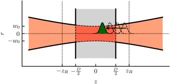
Figure 1: Schematic view of the focal geometry: The laser beam (orange) intersects the gas-target beam (gray), which is assumed to possess a uniform density distribution. If the diameter of the gas-target beam, $D$, is smaller than twice the Rayleigh length of the focus, $z_{R}$, the effective focal volume can be approximately described with a constant radial standard deviation, $\sigma_{r}=w_{0}/2$. The spatial equivalent of the laser pulse’s temporal distribution for a distinct time is a Gaussian profile (green). Since neither the longitudinal nor the radial intensity distribution change upon the pulse’s passage through the focal volume, the whole space- and time-integrated laser-target interaction can be described by a spheroidal intensity function, see (1).

After rearrangement of (1) to

$$\frac{r^{2}}{\sigma_{r}^{2}}+\frac{z^{2}}{\sigma_{z}^{2}}=2\,\ln\frac{I_{0}}{I},$$ (2)

it is obvious that points of equal intensity are located on the surface of a spheroid. Accordingly, the volume function is

$$V_{\text{3D}}(I)=\frac{4\pi}{3}\sigma_{r}^{2}\sigma_{z}\left(2\ln\frac{I_{0}}{I}\right)^{3/2}$$ (3)

with the differential volume $-({\partial{V_{\text{3D}}}}/{\partial{I}})\operatorname{d\!}{I}$ that is occupied by the iso-intensity shell $\operatorname{d\!}{I}$ around $I$ following

$$-\frac{\partial V_{\text{3D}}}{\partial I}\operatorname{d\!}{I}\propto\frac{\sqrt{\text{ln}\frac{I_{0}}{I}}}{I}\operatorname{d\!}{I}.$$ (4)

This provides a measure for the weight of any intensity between 0 and $I_{0}$ in the laser–target interaction. It complements the previous elaborations Wang et al. (2005) by the additional consideration of the laser pulse’s temporal intensity profile. Note that the description of the volume function $V_{\text{3D}}$ will only be as simple as (3) if the radial intensity distribution is independent of $z$, i. e., $D<2z_{R}$.

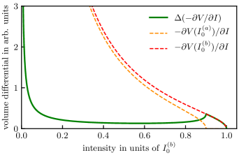
Figure 2: Intensity-dependent volume differentials for a space- and time-integrated laser–target interaction in a 3D configuration for two peak intensities $I_{0}^{(a)}/I_{0}^{(b)}=0.9$ (dashed lines). The difference between the two volume differentials (solid line) exhibits highly suppressed intensity contributions for $I<I_{0}^{(a)}$.

Fig. 2 shows the resulting intensity spectra for two peak intensities $I_{0}^{(a)}/I_{0}^{(b)}=0.9$ along with the corresponding difference spectrum. Evidently, in the difference spectrum the contributions from intensities $<I_{0}^{(a)}$ are highly suppressed, albeit not completely eliminated. The pole point at $I=0$ does not affect the determination of any intensity-dependent quantity, because the corresponding signal scales with $\Delta(-\partial V_{\text{3D}}/\partial I)\cdot{}I^{n}$, $n>0$. Here, $n$ would be an integer for a pure single-channel multiphoton process but does rather represent an intensity-dependent quantity for a realistic strong-field interaction.

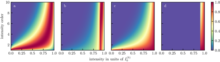
Figure 3: Normalized signals as a function of intensity and intensity order $n$ for different volume differentials: a) full volume in 3D configuration, b) differential volume in 3D configuration, c) full volume in 2D configuration, d) differential volume in 2D configuration. These provide a measure for the relative contribution of a distinct intensity to an overall signal, that scales with intensity to the power of a fixed exponent. For the differential-volume signals a ratio of $Q=I_{0}^{(a)}/I_{0}^{(b)}=0.9$ was used, which represents the lowest $Q$ value employed in experiment. All signal maps depicted were row-wise normalized to their maxima. For the 2D configuration case the volume differential follows $-{\partial V_{\text{2D}}/\partial I}\propto-{1/I}$ Wang et al. (2005).

The full-volume and exemplary difference signals are shown in Fig. 3 for both, the 2D and the 3D configuration, as a function of intensity and intensity order $n$. Note that for a focal interaction with intensities normally distributed only along two dimensions (2D configuration), i. e., either a spatial laser sheet with a Gaussian temporal profile or a two-dimensional spatial profile with a flat-top temporal profile, the corresponding difference intensity spectrum carries non-zero contributions only for $I_{0}^{(a)}\leq{}I<I_{0}^{(b)}$.

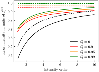
Figure 4: Mean intensity as a function of the intensity order $n$ for different intensity-difference signals with peak-intensity ratios $Q=I_{0}^{(a)}/I_{0}^{(b)}$ for the 3D (solid lines) and 2D configurations (dashed lines). The black lines correspond to signals at full volume integration, $Q=0$, i. e., evaluated at a single peak intensity. $Q$ values of $0.9$ and $0.99$ represent the lower and upper limits of peak-intensity ratios used in our experiments, vide infra.

Fig. 4 displays the mean intensities for various intensity-difference signals in dependence of the intensity order. In general, the use of a 2D focus configuration gives rise to mean intensities that are closer to the peak intensity compared to the 3D case. The black lines illustrate the change of the mean intensity with increasing intensity order for measurements at a single peak intensity. Especially for low intensity orders the corresponding mean intensities are far below the (upper) peak intensity. In contrast, in an intensity-difference setup the situation is much better, further improving with rising peak-intensity ratios $Q=I_{0}^{(a)}/I_{0}^{(b)}$. The green graphs, $Q=0.99$, provide insight into the achievable mean intensity for $Q\to 1$: for the 2D configuration the mean intensity reflects, almost independently of the intensity order, the actual peak intensity. However, for the 3D case there is an appreciable deviation, especially for signals that arise at low intensity orders. Furthermore, as $Q$ increases, the fractional signal that is kept with respect to the full signal at peak intensity becomes smaller.

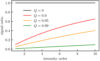
Figure 5: Fraction of the intensity-difference signal of the overall signal at peak intensity. 2D and 3D configuration show identical behavior.

This behavior is depicted in Fig. 5 and is identical for 2D and 3D configurations. In actual experiments one needs to find a compromise between intensity resolution and remaining signal.

In the following paragraph intensity-integrated observables and their derivatives with respect to peak intensity are elucidated. Any $M$-dimensional observable $S(I_{0})$, e. g., a two-dimensional projection of photoelectron momenta, that results from the full laser–target interaction at peak intensity $I_{0}$, obeys the relation

$$S(I_{0})\propto\int_{0}^{I_{0}}\Omega(I)s(I)\left(-\frac{\partial V}{\partial I}\right)\operatorname{d\!}{I},$$ (5)

with a normalized $M$-dimensional distribution $s(I)$ that is created at the distinct intensity $I$ with probability $\Omega(I)$ and the volume $-(\partial V/\partial I)\operatorname{d\!}{I}$ occupied by the iso-intensity shell d$I$. If $-(\partial V/\partial I)\operatorname{d\!}{I}$ is independent of $I_{0}$ (2D configuration), the evaluation of $\operatorname{d\!}{S}/\operatorname{d\!}{I_{0}}$ enables the direct determination of $\Omega(I)s(I)$ by elimination of the integral sign in (5). This is not viable for the 3D configuration, since the volume differential is a function of $I_{0}$. But also for this case $\operatorname{d\!}{S}/\operatorname{d\!}{I_{0}}$ is proportional to an effective distribution $\tilde{s}$, that arises from a restricted intensity spectrum as depicted in Fig. 2 and 3. Thus, the acquisition of $\operatorname{d\!}{S}/\operatorname{d\!}{I_{0}}$, or its discrete equivalent $\Delta S/\Delta I_{0}$, allows for the investigation of intensity-dependent changes in the signal distribution, while intensity-dependent occurrence probabilities, $\Omega(I)$, are not accessible.

Although a 2D focus configuration would enable the determination of intensity-dependent ionization rates as well as momentum distributions without contamination from intensities $I<I_{0}^{(a)}$, the experimental realization of such a setup suited for intensities appropriate for strong-field ionization studies proves to be challenging. However, the evaluation of $\Delta{S}/\Delta{I_{0}}$ in a 3D configuration is easy to implement and provides the investigator with incident-intensity resolved signal distributions $\tilde{s}$. This enables analyses of the intensity-dependence of an $M$-dimensional signal, while the information about the integral signal remains obscured.

III Experimental setup

The experimental setup was described elsewhere Trippel et al. (2013); Chang et al. (2015). In brief, a cold molecular beam was created by supersonically expanding OCS seeded in 85 bar of helium through an Even-Lavie valve Even et al. (2000) operated at a repetition rate of 250 Hz. The skimmed molecular beam was intersected in the center of a velocity-map imaging spectrometer by a laser beam from a mode-locked Ti:sapphire system, which delivered Fourier-limited pulses at 800 nm central wavelength and 35 fs pulse duration (full width at half maximum) at a repetition rate of 1 kHz. Employing a 500 mm focal length biconvex lens resulted in a laser focus with a beam waist of 44 µm and a Rayleigh length of $z_{R}=7.5$ mm. The diameter of the molecular beam was found to be $D=2.2$ mm and $2z_{R}>D$ provides justification for treating the longitudinal intensity distribution of the effective focus as a rectangular function in the previous section. The pulse energy reaching the interaction region was defined using a half-wave plate and a thin-film polarizer. Ionization of OCS could be studied employing peak intensities of $4.6\text{--}13\times 10^{13}~{}\text{W}/\text{cm}^{2}$, respectively. Due to the charge-dissipation limit of the in-vacuum detector components measurements at $I_{0}>8\times 10^{13}~{}\text{W}/\text{cm}^{2}$ were conducted at a reduced sample density – namely $1/3$ of the density employed for measurements at $I_{0}\leq 8\times 10^{13}~{}\text{W}/\text{cm}^{2}$. This was achieved by delaying the laser pulses with respect to the maximum of the molecular beam’s temporal profile. Sample densities of $1\times 10^{8}$ cm^-3 and $1/3\times 10^{8}$ cm^-3 were utilized, respectively. Peak intensities as determined by a combination of beam-profiling, auto-correlation, and measurement of the pulse energy were found to be too low by $20~{}\%$ compared to the intensity-dependent kinetic energy shift of distinct above-threshold ionization (ATI) peaks, see (8). In combination with the known energy spacing between adjacent ATI peaks, namely the photon energy $h\nu$, this approach allowed for an intrinsic calibration of both, the photoelectron momentum and the laser intensity. Two-dimensional projections of photoelectron momenta were recorded by mapping the electrons onto a position-sensitive detector, consisting of a microchannel plate (MCP), a phosphor screen and a high-frame-rate camera (Optronis CL600), by means of a velocity map imaging spectrometer (VMIS). This detection scheme allowed for counting and two-dimensional momentum-stamping of single electrons. The momentum resolution achieved – given by the voltage applied to the VMIS electrodes and the pixel size of the camera – was $5.6\times 10^{-3}$ atomic units (electron velocity of 12 km/s). Momentum slices of the full three-dimensional momentum distributions $S(I_{0})$ were recovered through inverse Abel-transformations employing the “Onion-Bordas” onion-peeling algorithm Bordas et al. (1996); Rallis et al. (2014) as implemented in the PyAbel software package Hickstein et al. (2016).

IV Results and Discussion

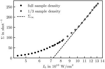
Figure 6: Experimental electron count rates versus the peak intensity on a semi-logarithmic scale (dots). Open dots represent measurements conducted at 1/3 of the maximum sample density rescaled accordingly to match those recorded at full density. The asymptotic behavior beyond the saturation intensity is depicted by the dashed line.

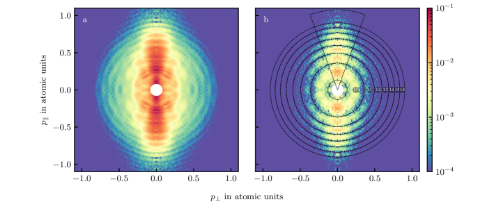
Figure 7: Photoelectron momentum slices a) for the full-intensity distribution $S$ at a peak intensity of $5.7\times 10^{13}~{}\text{W}/\text{cm}^{2}$ and b) for the differential-intensity distribution $S^{\prime}$, which is dominated by intensities of $5.4\text{--}5.7\times 10^{13}~{}\text{W}/\text{cm}^{2}$. The black-line wedge sketches the polar angles used to evaluate the intensity-dependent radial distributions shown in Fig. 8 and 9; the black circles separate contributions from distinct photon numbers $N$ and correspond to kinetic energies $T(N\pm 0.5,\tilde{I}_{0})$ as obtained from (8).

IV.1 Integral photoelectron yield

Extensive strong-field ionization studies Hankin et al. (2001) employing various laser peak intensities demonstrated that the asymptotic slope of an integral ionization signal $\Sigma(I_{0})$ with respect to $\ln{I_{0}}$, arising from the full intensity spectrum of the laser–target interaction at peak intensity $I_{0}$, follows

$$\lim_{I_{0}\to\infty}\left(\frac{\operatorname{d\!}{\Sigma}}{\operatorname{d\!}\ln{I_{0}}}\right)=2\pi\alpha\sigma_{r}^{2}D\varrho\,.$$ (6)

$\alpha$ is the instrument sensitivity, $\sigma_{r}$ the standard deviation of the transverse intensity distribution, $D$ the length of the focus volume and $\varrho$ the sample density. The only requirements for the validity of this equation are the predominance of single ionization and the cylindrical symmetry of the spatial focus geometry. Due to the onset of saturation, starting at intensity $I_{\text{sat}}$, the slope of $\Sigma(\ln{I_{0}})$ converges to a constant value for increasing peak intensity. Within the notation of this manuscript $\Sigma(I_{0})$ equals the momentum-space integral of the distribution $S(I_{0})$, which for the present case is just the total number of electrons detected. Fig. 6 shows the resulting values of $\Sigma$ plotted versus $I_{0}$ on a semi-logarithmic scale. With increasing values of $\text{ln}I_{0}$ the slope of the total electron yield converges to a constant value. In the following analysis, this behavior is used as implicit evidence for a negligible contribution from multiple ionization. The asymptotic slope and the saturation onset were deduced by modeling a line through the highest peak-intensity points providing a saturation onset of $I_{\text{sat}}=7.2\times 10^{13}~{}\text{W}/\text{cm}^{2}$. The saturation intensity is a function of both, the pulse duration and the orientation-dependent ionization probability Hankin et al. (2001). Using the MCP’s open area ratio of 0.64 as instrument sensitivity $\alpha$, a transverse focal standard deviation of $\sigma_{r}=22~{}\text{\textmu{m}}$ (beam waist of 44 µm) and a molecular beam diameter of $D=2.2$ mm resulted in a sample density of $\varrho=1\times 10^{8}~{}\text{W}/\text{cm}^{3}$. Since the intensity could be intrinsically calibrated from the ponderomotive shift of the ATI peaks (see next subsection), the deduced sample density is as accurate as $\alpha\sigma_{r}^{2}D$.

IV.2 Radial and angular distributions

Due to their rotational symmetry the three-dimensional momentum distributions $S(I_{0})$ can be completely described by two-dimensional slices of momenta parallel ($p_{\parallel}$) and perpendicular ($p_{\bot}$) to the polarization axis. In the following, the slope of $S$ with respect to $I_{0}$,

$$S^{\prime}(\tilde{I}_{0})=\frac{\Delta S}{I_{0}^{(b)}-I_{0}^{(a)}}\,,$$ (7)

is analyzed regarding its radial and angular distributions. Here, the mean intensity $\tilde{I}_{0}$ corresponds to the arithmetic mean of every two peak intensities $I_{0}^{(b)}>I_{0}^{(a)}$ that were used to measure $S$. Since $S^{\prime}(\tilde{I}_{0})$ arose from a more narrow distribution of incident intensities than $S(I_{0})$, it allows for the detailed investigation of intensity dependent effects.

Both $S(I_{0})$ and $S^{\prime}(\tilde{I}_{0})$ exhibit rich angular and radial structure. Fig. 7 displays a typical momentum slice for the two cases, here for intensities around $5.5\times 10^{13}~{}\text{W}/\text{cm}^{2}$. Both momentum distributions show broad radial patterns that repeat with integer multiples of the photon energy – referred to as ATI structure –, sharp radial features on top of the ATI structures – referred to as Freeman resonances Freeman et al. (1987) – and a carpet-like pattern perpendicular to the polarization axis Korneev et al. (2012).

IV.2.1 Radial distributions

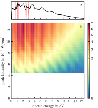
Figure 8: Radial distributions of $S(I_{0})$ were evaluated for polar angles in $[\!-20\,^{\circ},\!+20\,^{\circ}]$ as sketched in Fig. 7 b: a) intensity-integrated radial distribution carrying imprints of Freeman resonances with principal quantum numbers $n=4,5,7,8$ indicated for $k=1$ (solid red lines) and $k=2$ (dashed red lines) as obtained through (9) and b) peak-intensity-dependent radial distributions. Values of $S(I_{0})$ are mapped onto a square-root color scale.

In Fig. 8 the peak-intensity dependent radial distributions for polar angles between $\!-20\,^{\circ}$ and $\!+20\,^{\circ}$ with respect to the polarization axis are illustrated for $S(I_{0})$. There are two kinds of features to be noted: (i) broad peaks with a spacing of $h\nu$ that experience a shift in kinetic energy proportional to the negative value of the peak intensity and (ii) sharp peaks at constant kinetic energies. The radial distributions of $S(I_{0})$ are dominated by feature (ii).

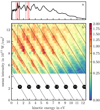
Figure 9: Radial distributions of $S^{\prime}(\tilde{I}_{0})$ were evaluated for polar angles in $[-20^{\circ},+20^{\circ}]$ as sketched in Fig. 7 b: a) intensity-integrated radial distribution and b) intensity-dependent radial distributions. Broken black lines in b) depict ponderomotively shifted final kinetic energies as obtained through (8) for the given numbers of photons. Values of $S^{\prime}(\tilde{I}_{0})$ are mapped onto a square-root color scale.

Fig. 9 displays the equivalent radial distributions for $S^{\prime}(\tilde{I}_{0})$, which exhibit predominant contributions from feature (i). Note that there is a change in sample density and intensity bin size at $8.3\times 10^{13}~{}\text{W}/\text{cm}^{2}$, c. f. Fig. 6 .

In the following, feature (i), which corresponds to non-resonant above-threshold ionization, is analyzed employing the radial distributions of $S^{\prime}(\tilde{I}_{0})$. Dashed black lines in Fig. 9 correspond to final kinetic energies Freeman and Bucksbaum (1991)

$$T(N,\tilde{I}_{0})=Nh\nu-{}I_{\text{p}}^{(0)}-\!~{}U_{\text{p}}(\tilde{I}_{0})\,,$$ (8)

with the number of absorbed photons $N$, the photon energy $h\nu=1.55$ eV, the field-free ionization potential of OCS, ${}I_{\text{p}}^{(0)}=11.19$ eV Linstrom and Mallard (2017), and the ponderomotive potential $\!~{}U_{\text{p}}=\tilde{I}_{0}/4\omega^{2}$ (for atomic units). Clearly, (8) describes the kinetic energies of the radial local maxima in Fig. 9 quite well except for minor deviations towards lower kinetic energies at $T<3$ eV, which are ascribed to the Coulomb interaction between photoelectron and cation. Thus, the total ionization energy appears to be dictated by the ponderomotive continuum shift. For the intensity range of the current study the relative Stark shift between the neutral and the cationic species is dominated by the permanent-dipole interaction Holmegaard et al. (2010) and, hence, equals zero in average over the isotropic distribution of molecular orientations.

Within the peak-intensity range investigated all radial distributions of $S(I_{0})$ carry series of sharp peaks, feature (ii), that are also reproduced periodically with the photon energy $h\nu$. Close inspection of Fig. 9 reveals that the kinetic energies of those peak series are independent of the incident intensity, i. e., they appear as vertical lines imprinted onto the non-resonant ATI pattern, feature (i). Based on this intensity-independence and the energy spacing between individual series, these peaks can unambiguously be assigned to Freeman resonances Freeman et al. (1987), i. e., photoelectron emission from resonance-enhanced multiphoton ionization through Rydberg states. Since those Rydberg states experience the same ac Stark shift as their corresponding continua, namely the ponderomotive energy, the resulting final kinetic energies $T_{\text{F}}$ are independent of the incident intensity Freeman and Bucksbaum (1991); O’Brian et al. (1994):

$$T_{\text{F}}(k,n)=kh\nu-\frac{R_{\infty}}{\left(n+0.25\right)^{2}}\,,$$ (9)

with the number of photons $k$ that ionize a resonant Rydberg state with principal quantum number $n$ and the Rydberg constant $R_{\infty}$. The subtrahend reflects the energy difference between the Rydberg state and its asymptotic unbound state. Resonant transitions for $n$ = 4, 5, 7 could be observed together with a combination band for $n$ = 8–10, with $k$ = 1–3. These assignments agree with previous single-photon absorption studies on OCS Tanaka et al. (1960); Sunanda et al. (2012); Cossart-Magos et al. (2003). In the present study individual angular momentum states could not be resolved: at a kinetic energy of 1.2 eV, where the $k=1$ Freeman manifold occurred, an energy resolution of 0.05 eV was achieved, which is roughly ten times larger than what would be required to distinguish between different $l$ states.

Previous results on OCS for comparable peak intensities of $2.8$–$9.4\times 10^{13}~{}\text{W}/\text{cm}^{2}$, analyzed without the intensity-difference spectra, lacked information about the incident ponderomotive shift and, hence, assigned intensity-independent photoelectron lines to valence–valence transitions Yu et al. (2017). Three sharp peaks in the photoelectron kinetic energy spectra, which follow $T_{1,3}=0.73\text{~{}eV}+\tilde{k}h\nu$, with $\tilde{k}=(0,1)$, and $T_{2}=1.17\text{~{}eV}$, were attributed to the valence transitions ${}^{1}\Delta\leftarrow\tilde{X}{{}^{1}\Sigma^{+}}$ and ${}^{1}\Pi\leftarrow\tilde{X}{{}^{1}\Sigma^{+}}$. The corresponding excited valence states have field-free vertical ionization energies of roughly 5.8 eV (${}^{1}\Delta$) and 3.9 eV (${}^{1}\Pi$) Sunanda et al. (2012). Both, the ${}^{1}\Delta$ and the ${}^{1}\Pi$ state, were considered to experience ac Stark shifts equal to the ponderomotive potential, resulting in intensity-independent kinetic energy releases Yu et al. (2017). Since $\!~{}U_{\text{p}}$ is the kinetic energy imparted to an unbound electron in an oscillating electric field, it represents the asymptotic ac Stark shift of an electronic state at the onset of the continuum. However, treating the ${}^{1}\Delta$ and ${}^{1}\Pi$ states as quasi-unbound states is in conflict with their large binding energies. Thus, in our present investigation the very same three peaks are, instead, assigned to ionization of resonant Rydberg states leading to final kinetic energies of $T_{1,3}=T_{\text{F}}(k=(1,2),n=4)$ and $T_{2}=T_{\text{F}}(k=1,n=7)$.

While $S^{\prime}(\tilde{I}_{0})$ mainly carries contributions from non-resonant above-threshold ionization, $S(I_{0})$ is dominated by resonance-enhanced multi-photon ionization. Through averaging over all intensities present in the focal volume the ponderomotively shifted non-resonant contributions get washed out in the final momentum distribution $S(I_{0})$, while resonant contributions with constant final momentum, e. g., Freeman resonances, gain intensity Rudenko et al. (2004). By inspection of $S(I_{0})$ only, the contributions from resonant ionization pathways are highly overestimated and final kinetic energies cannot be related to distinct numbers of absorbed photons, because the ponderomotive continuum shift $\!~{}U_{\text{p}}$ cannot be resolved. In the momentum distributions $S(I_{0})$ the closing of ionization channels with increasing peak intensities is highly obscured, because contributions from all intensities between 0 and $I_{0}$ are contained. Thus, even if a channel is already closed at the peak intensity, $S(I_{0})$ will embody all contributions from $I<I_{0}$ with even larger weight, i. e., larger differential volume, at which the channel is still open. In principle, $S(I_{0})$ contains just more and more open ionization channels with increasing peak intensity. Nevertheless, experimental evidence for channel-closing was reported for xenon at fully focal-volume averaged momentum distributions Schyja et al. (1998); Li et al. (2015). In the present study, three channel-closings could be clearly observed, visible in Fig. 9 at intensities when the ATI peaks assume zero kinetic energy.

IV.2.2 Angular distributions

In the following, the non-resonant ATI channels for ionization with a minimum number of photons are analyzed with respect to their photoelectron angular distributions. These channels give rise to the lowest radial layers of the carpet-like pattern Korneev et al. (2012) visible in Fig. 7 a. The minimum number of photons needed to ionize the target is a staircase function proceeding upward with increasing intensity. Accordingly, $S^{\prime}(\tilde{I}_{0})$ was sectioned by the channel-closing intensities, which were obtained by evaluating the roots of (8). Within the intensity range investigated the closing of the $9,10,11,12$ photon channels were encountered at intensities of $4.6,7.2,9.8,12.4\times 10^{13}~{}\text{W}/\text{cm}^{2}$, respectively.

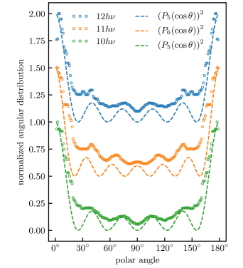
Figure 10: Angular distributions of the lowest order non-vanishing ATI channels for the minimum numbers of photons of $10,11,12$ required to ionize the OCS molecule. The three distributions were retrieved within the intensity intervals $[4.6,7.2[,[7.2,9.8[,[9.8,12.4[\times 10^{13}~{}\text{W}/\text{cm}^{2}$, which represent the channel-closing intensities obtained by setting $T(N,\tilde{I}_{0})=0$ in (8). Experimental data are shown by circles, calculated traces of the squares of Legendre polynomials $P_{l}(\cos\theta)$ of order $l$ with the polar angle $\theta$ to the laser polarization axis are shown by dashed lines. The distributions are plotted with an arbitrary vertical offset for clarity.

In Fig. 10 , circles depict the resulting angular distributions for ionization by $10,11,12$ photons, each representing the lowest order non-vanishing ATI channel in its corresponding intensity regime. The angular distributions associated with the absorption of $10,11,12$ photons exhibit $5,6,5$ local minima, respectively.

As shown by a theoretical study of the strong-field ionization of atomic hydrogen Arbó et al. (2006) and by experimental investigations of xenon Li et al. (2015), the dominant orbital angular momentum quantum number $l$ of the emitted electrons can be deduced from fitting the angular distributions by squared Legendre polynomials $\left(P_{l}(\cos\theta)\right)^{2}$ of order $l$. According to the number of local minima the absorption of $N=10,11,12$ photons gives rise to dominant orbital angular momentum quantum numbers of $l=5,6,5$. Best matches of $\left(P_{l}(\cos\theta)\right)^{2}$ to the experimental angular distributions are shown as dashed lines in Fig. 10 .

An empirical rule was given that predicts the dominant photoelectron orbital angular momentum quantum number $l$ based only on the minimum number of photons to reach the continuum and the orbital quantum number $l_{0}$ of the initial bound electronic state Chen et al. (2006). For intensities implying minimum numbers of $10,11,12$ photons needed to ionize argon, ground state configuration [Ne]$3s^{2}3p^{6}~{}(l_{0}=1)$, dominant orbital-angular-momentum quantum numbers of $l=5,6,5$ were found. These values for $l$ agree with those obtained for OCS, ground state configuration $\ldots 9\sigma^{2}{}3\pi^{4}~{}(l_{0}=1)$, providing clear evidence of the empirical rule and its extension to molecules.

The time-dependent Schrödinger equation for the strong-field ionization of H and Ar pictured the trajectory of the outgoing electron as a quiver motion along the laser-polarization axis superimposed to a drift motion following a Kepler hyperbola Arbó et al. (2008). Identifying the hyperbola’s pericenter as the electron’s quiver amplitude in the field provided an analytical expression for an effective final orbital momentum that – for single ionization – only depends on the electron’s final linear momentum and its quiver amplitude in the field. For the ionization of OCS through $10,11,12$ photons effective orbital quantum numbers $\tilde{l}=5.5,6.5,7.1$ were obtained accordingly Arbó et al. (2008). Although this model considers neither the initial state’s orbital momentum nor a parity selection rule, the values for $\tilde{l}$ reflect our experimental observations remarkably well. This further supports the statement that the momentum distribution of an electron wave packet from non-resonant strong-field ionization is dictated by the electric field and its Coulomb interaction with the cation. The initial bound electronic state imprints onto the free-electron wave packet through its vertical ionization energy, its orbital angular momentum, and the symmetry of its electron density distribution. While the impact of the former two properties was demonstrated within the scope of this manuscript, the investigation of the latter would require referencing to the molecular frame.

V Conclusions

Three-dimensional photoelectron momentum distributions from strong-field ionization of OCS at differential peak intensities were recorded and analyzed in matters of resonant Rydberg states and photoelectron angular momentum. The evaluation of the derivatives of the momentum distributions with respect to the peak intensity allowed for the unambiguous recognition of Freeman resonances. As a result, sharp photoelectron lines, previously ascribed to valence-valence transitions Yu et al. (2017), were reassigned to progressions of Freeman resonances corresponding to Rydberg states with principal quantum numbers $n=4,5,7,8,9,10$. Furthermore, the empirical rule that relates the initial state’s angular momentum and the minimum photon expense to ionize an ac Stark shifted atomic system to the observable dominant photoelectron momentum Chen et al. (2006) could be confirmed for a molecular target. In addition, the clear closing of ionization channels with increasing peak intensity is shown for the OCS molecule, which could eventually enable the probing of a distinct strong-field ionization channel in a coherent-control experimental setup. It is demonstrated that in order to gain insight into strong-field ionization processes on a quantum-mechanical level it is essential to relate distinct incident intensities to the resulting response of the system under investigation. Especially for the exploration of the transition regime between multi-photon and tunneling ionization a well-defined and narrow intensity distribution is crucial. Studies employing a clear relation between incident intensity and target response could finally shed light onto the importance of resonant states and, thus, show the shortcomings of present molecular strong-field ionization theories to describe the outgoing electron wave packet.

References

- Hankin et al. (2001) S. Hankin, D. Villeneuve, P. Corkum, and D. Rayner, “Intense-field laser ionization rates in atoms and molecules,” Phys. Rev. A 64, 013405 (2001).
- Hart et al. (2014) N. A. Hart, J. Strohaber, G. Kaya, N. Kaya, A. A. Kolomenskii, and H. A. Schuessler, “Intensity-resolved above-threshold ionization of xenon with short laser pulses,” Phys. Rev. A 89, 1393 (2014).
- Shao et al. (2015) Y. Shao, M. Li, M. M. Liu, X. Sun, X. Xie, P. Wang, Y. Deng, C. Wu, Q. Gong, and Y. Liu, “Isolating resonant excitation from above-threshold ionization,” Phys. Rev. A 92, 2008 (2015).
- Yu et al. (2017) J. Yu, W. Hu, X. Li, P. Ma, L. He, F. Liu, C. Wang, S. Luo, and D. Ding, “Contribution of resonance excitation on ionization of OCS molecules in strong laser fields,” J. Phys. B 50, 235602 (2017).
- Li et al. (2015) M. Li, P. Zhang, S. Luo, Y. Zhou, Q. Zhang, P. Lan, and P. Lu, “Selective enhancement of resonant multiphoton ionization with strong laser fields,” Phys. Rev. A 92, 1945 (2015).
- Schyja et al. (1998) V. Schyja, T. Lang, and H. Helm, “Channel switching in above-threshold ionization of xenon,” Phys. Rev. A 57, 3692–3697 (1998).
- Marchenko et al. (2010) T. Marchenko, H. G. Muller, K. J. Schafer, and M. J. J. Vrakking, “Electron angular distributions in near-threshold atomic ionization,” J. Phys. B 43, 095601 (2010).
- Holmegaard et al. (2010) L. Holmegaard, J. L. Hansen, L. Kalhøj, S. L. Kragh, H. Stapelfeldt, F. Filsinger, J. Küpper, G. Meijer, D. Dimitrovski, M. Abu-samha, C. P. J. Martiny, and L. B. Madsen, “Photoelectron angular distributions from strong-field ionization of oriented molecules,” Nat. Phys. 6, 428 (2010), arXiv:1003.4634 [physics] .
- Dimitrovski et al. (2015) D. Dimitrovski, J. Maurer, H. Stapelfeldt, and L. B. Madsen, “Strong-field ionization of three-dimensionally aligned naphthalene molecules: orbital modification and imprints of orbital nodal planes,” J. Phys. B 48, 245601 (2015).
- Maurer et al. (2012) J. Maurer, D. Dimitrovski, L. Christensen, L. B. Madsen, and H. Stapelfeldt, “Molecular-frame 3d photoelectron momentum distributions by tomographic reconstruction,” Phys. Rev. Lett. 109, 123001 (2012).
- Ivanov et al. (2005) M. Y. Ivanov, M. Spanner, and O. Smirnova, “Anatomy of strong field ionization,” J. Mod. Opt. 52, 165–184 (2005).
- Ammosov et al. (1986) M. V. Ammosov, N. B. Delone, and V. P. Krainov, “Tunnel ionization of complex atoms and of atomic ions in an alternating electromagnetic field,” Soviet Physics - JETP 64, 1191–1194 (1986).
- Walker et al. (1998) M. A. Walker, P. Hansch, and L. D. Van Woerkom, “Intensity-resolved multiphoton ionization: Circumventing spatial averaging,” Phys. Rev. A 57, R701–R704 (1998).
- Wang et al. (2005) P. Wang, A. M. Sayler, K. D. Carnes, B. D. Esry, and I. Ben-Itzhak, “Disentangling the volume effect through intensity-difference spectra: application to laser-induced dissociation of H,” Opt. Lett. 30, 664 (2005).
- Strohaber et al. (2010) J. Strohaber, A. A. Kolomenskii, and H. A. Schuessler, “Reconstruction of ionization probabilities from spatially averaged data in dimensions,” Phys. Rev. A 82, 013403 (2010).
- Trippel et al. (2013) S. Trippel, T. Mullins, N. L. M. Müller, J. S. Kienitz, K. Długołęcki, and J. Küpper, “Strongly aligned and oriented molecular samples at a kHz repetition rate,” Mol. Phys. 111, 1738 (2013), arXiv:1301.1826 [physics] .
- Chang et al. (2015) Y.-P. Chang, D. A. Horke, S. Trippel, and J. Küpper, “Spatially-controlled complex molecules and their applications,” Int. Rev. Phys. Chem. 34, 557–590 (2015), arXiv:1505.05632 [physics] .
- Even et al. (2000) U. Even, J. Jortner, D. Noy, N. Lavie, and N. Cossart-Magos, “Cooling of large molecules below 1 K and He clusters formation,” J. Chem. Phys. 112, 8068–8071 (2000).
- Bordas et al. (1996) C. Bordas, F. Paulig, H. Helm, and D. L. Huestis, “Photoelectron imaging spectrometry: Principle and inversion method,” Rev. Sci. Instrum. 67, 2257 (1996).
- Rallis et al. (2014) C. E. Rallis, T. G. Burwitz, P. R. Andrews, M. Zohrabi, R. Averin, S. De, B. Bergues, B. Jochim, A. V. Voznyuk, N. Gregerson, B. Gaire, I. Znakovskaya, J. McKenna, K. D. Carnes, M. F. Kling, I. Ben-Itzhak, and E. Wells, “Incorporating real time velocity map image reconstruction into closed-loop coherent control,” Rev. Sci. Instrum. 85, 113105 (2014).
- Hickstein et al. (2016) D. D. Hickstein, R. Yurchak, D. Dhrubajyoti, C.-Y. Shih, and S. T. Gibson, “PyAbel (v0.7): A Python Package for Abel Transforms,” (2016).
- Freeman et al. (1987) R. R. Freeman, P. H. Bucksbaum, H. Milchberg, S. Darack, D. Schumacher, and M. E. Geusic, “Above-threshold ionization with subpicosecond laser pulses,” Phys. Rev. Lett. 59, 1092–1095 (1987).
- Korneev et al. (2012) P. A. Korneev, S. V. Popruzhenko, S. P. Goreslavski, T.-M. Yan, D. Bauer, W. Becker, M. Kübel, M. F. Kling, C. Rödel, M. Wünsche, and G. G. Paulus, “Interference Carpets in Above-Threshold Ionization: From the Coulomb-Free to the Coulomb-Dominated Regime,” Phys. Rev. Lett. 108, 223601 (2012).
- Freeman and Bucksbaum (1991) R. R. Freeman and P. H. Bucksbaum, “Investigations of above-threshold ionization using subpicosecond laser pulses,” J. Phys. B 24, 325–347 (1991).
- Linstrom and Mallard (2017) P. J. Linstrom and W. G. Mallard, eds., NIST Chemistry WebBook, NIST Standard Reference Database Number 69 (National Institute of Standards and Technology, Gaithersburg MD, 20899, 2017).
- O’Brian et al. (1994) T. R. O’Brian, J.-B. Kim, G. Lan, T. J. McIlrath, and T. B. Lucatorto, “Verification of the ponderomotive approximation for the ac Stark shift in Xe Rydberg levels,” Phys. Rev. A 49, R649–R652 (1994).
- Tanaka et al. (1960) Y. Tanaka, A. S. Jursa, and F. J. LeBlanc, “Higher ionization potentials of linear triatomic molecules. II. CS2, COS, and N2O,” J. Chem. Phys. 32, 1205–1214 (1960).
- Sunanda et al. (2012) K. Sunanda, B. N. Rajasekhar, P. Saraswathy, and B. N. Jagatap, “Photo-absorption studies on carbonyl sulphide in 30,000–91,000 cm-1 region using synchrotron radiation,” J. Quant. Spectrosc. Radiat. Transf. 113, 58–66 (2012).
- Cossart-Magos et al. (2003) C. Cossart-Magos, M. Jungen, R. Xu, and F. Launay, “High resolution absorption spectrum of jet-cooled OCS between 64 000 and 91 000 cm-1,” J. Chem. Phys. 119, 3219–3233 (2003).
- Rudenko et al. (2004) A. Rudenko, K. Zrost, C. D. Schröter, V. L. B. De Jesus, B. Feuerstein, R. Moshammer, and J. Ullrich, “Resonant structures in the low-energy electron continuum for single ionization of atoms in the tunnelling regime,” J. Phys. B 37, L407–L413 (2004).
- Arbó et al. (2006) D. G. Arbó, S. Yoshida, E. Persson, K. I. Dimitriou, and J. Burgdörfer, “Interference Oscillations in the Angular Distribution of Laser-Ionized Electrons near Ionization Threshold,” Phys. Rev. Lett. 96, 143003 (2006).
- Chen et al. (2006) Z. Chen, T. Morishita, A.-T. Le, M. Wickenhauser, X. M. Tong, and C. D. Lin, “Analysis of two-dimensional photoelectron momentum spectra and the effect of the long-range coulomb potential in single ionization of atoms by intense lasers,” Phys. Rev. A 74, 053405 (2006).
- Arbó et al. (2008) D. G. Arbó, K. I. Dimitriou, E. Persson, and J. Burgdörfer, “Sub-Poissonian angular momentum distribution near threshold in atomic ionization by short laser pulses,” Phys. Rev. A 78, 1418 (2008).