ULB-TH/19-01

A feeble window on leptophilic dark matter

Sam Junius$\,{}^{a,b,c}$, Laura Lopez-Honorez$\,{}^{a,b}$,
and Alberto Mariotti$\,{}^{b,c}$

^aService de Physique Théorique, Université Libre de Bruxelles, C.P. 225, B-1050 Brussels, Belgium ^bTheoretische Natuurkunde & The International Solvay Institutes, Vrije Universiteit Brussel, Pleinlaan 2, B-1050 Brussels, Belgium
^cInter-University Institute for High Energies, Vrije Universiteit Brussel, Pleinlaan 2, B-1050 Brussels, Belgium

In this paper we study a leptophilic dark matter scenario involving feeble dark matter coupling to the Standard Model (SM) and compressed dark matter-mediator mass spectrum. We consider a simplified model where the SM is extended with one Majorana fermion, the dark matter, and one charged scalar, the mediator, coupling to the SM leptons through a Yukawa interaction. We first discuss the dependence of the dark matter relic abundance on the Yukawa coupling going continuously from freeze-in to freeze-out with an intermediate stage of conversion driven freeze-out. Focusing on the latter, we then exploit the macroscopic decay length of the charged scalar to study the resulting long-lived-particle signatures at collider and to explore the experimental reach on the viable portion of the parameter space.

1 Introduction

As of today, the most conventional paradigm for dark matter (DM) has been the so-called Weakly Interacting Massive Particle (WIMP). WIMPs have been the main target of experimental searches, including collider experiments, direct and indirect DM detection. In the WIMP scenario, the DM is produced in the early Universe through the freeze-out mechanism, leading typically to the correct DM relic abundance for electroweak size couplings and masses. This is however not the only possibility to obtain the right DM abundance. By varying the DM mass, its coupling strength to the Standard Model (SM) and/or within the dark sector, one can generate DM through different mechanisms during the cosmological evolution of the Universe. Specifically, one can continuously go from freeze-out to freeze-in passing through several intermediate DM production regimes, see e.g. [1, 2, 3, 4]. In some parts of this parameter space, the DM happens to be very feebly coupled to the SM, i.e. with couplings much more suppressed than for the WIMP case.

We focus on this feeble interaction window for scenarios involving a small mass splitting between the dark matter and the mediator connecting DM to the SM. We will study in details the mechanism of dark matter production in the early universe, from freeze-in to freeze-out. In particular, we will mainly focus on the intermediate stage of DM coannihilation freeze-out happening out of chemical equilibrium (CE) with the SM plasma, also called conversion driven freeze-out. Such a scenario has already been pointed out in [3] and mainly studied for dark matter coupling to quarks [3, 5, 6]. Here instead we focus on the case of a leptophilic dark matter model. Conversion processes between the mediator and the dark matter will play a central role in defining the evolution of the DM abundance and they will have to be taken into account in the study of the DM/mediator Boltzmann equations. In passing, we will also emphasize the fact that, within the freeze-in framework, mediator scatterings (as opposed to decay) can play a leading role in determining the DM relic density. Finally, we will identify the viable parameter space for conversion driven freeze-out so as to further study the experimental constraints on this class of models.

The feeble coupling of the DM to the mediator allows for a macroscopic decay length of the mediator that can be observed at colliders through e.g. charged and/or disappearing tracks. These are typical features of DM scenarios in which the DM abundance results from the freeze-in [4] and conversion driven freeze-out [3]. These production mechanisms can lead to distinctive and challenging signatures at colliders, including long lived charged particles and very soft signatures. In the freeze-in case, the DM coupling is so suppressed that the mediator mainly decays outside the detector giving rise to charged tracks. For conversion driven freeze-out, the slightly larger couplings involved can also give rise to disappearing tracks. The LHC community has already provided a strong effort in the study of final state signatures which arise from DM models, focusing mainly on the WIMP scenario and on prompt missing energy signatures, see e.g. [7]. Recently, more attention has been devoted to long lived particle signatures arising in DM models, that we will study here, see e.g. [4, 8, 9, 10, 11, 12, 5, 13, 3, 14, 15, 16, 17, 18, 19, 20, 21, 22]. Notice that due to the feeble coupling involved, direct and indirect detection dark matter searches are challenging, see however e.g. [1, 23, 24, 25, 26, 27, 28, 29]. Unconventional signatures at the LHC can hence provide the main experimental probes for the class of model studied here.

The rest of the paper is organized as follows. In Sec. 2, we introduce the leptophilic DM model on which we focus all along this work. In Sec. 3, we detail the computation of the dark matter relic abundance in different regimes underlying the specificities of the compressed spectrum scenarios. In Sec. 4 we turn to the unexplored window on leptophilic DM provided by the conversion driven mechanism, determining the viable parameter space and the corresponding collider constraints. We summarize and conclude in Sec. 5, while we present some technical details in the Appendices.

2 The simplified leptophilic dark matter model

In this paper, we work in a minimal extension of the Standard Model (SM) involving a Majorana fermion $\chi$ dark matter coupled to SM leptons through the exchange of charged scalar mediator $\phi$. The Lagrangian encapsulating the BSM physics reads

$${\cal L}\supset\frac{1}{2}\bar{\chi}\gamma^{\mu}\partial_{\mu}\chi-\frac{m_{\chi}}{2}\bar{\chi}\chi+(D_{\mu}\phi)^{\dagger}\ D^{\mu}\phi-m_{\phi}^{2}|\phi|^{2}\ -\ \lambda_{\chi}\phi\bar{\chi}l_{R}\ +\ h.c.$$ (1)

where $m_{\chi}$ is the dark matter mass, $m_{\phi}$ is the mediator mass and $\lambda_{\chi}$ denotes the Yukawa coupling between the dark matter, the right handed SM lepton $l_{R}$ and the mediator. We have assumed that a $Z_{2}$ symmetry prevents the dark matter to decay directly to SM particles. Both $\chi$ and $\phi$ are odd under the $Z_{2}$ symmetry while the SM fields are even and we assume $m_{\phi}>m_{\chi}$.

(a)

(b)

Figure 1: The Feynman diagrams for the most important conversion processes.

The standard WIMP phenomenology of (1) has already been studied in length in [30, 31, 32, 33, 34, 35, 36] while the corresponding scalar DM case has been studied in [37, 38, 39, 40, 41, 42]. Here in contrast, we extend existing analysis to couplings $\lambda_{\chi}$ bringing the dark matter out of chemical equilibrium (CE) focusing on small mass splittings between the dark matter and the mediator. In this set-up, the conversion $\chi\leftrightarrow\phi$ processes depicted in Fig. 1 will play the leading roles. We will study how the phenomenology of the model (1) non-trivially evolves between the two extremes of freeze-in and standard freeze-out. For an interaction strength just below CE limit, i.e. couplings $\lambda_{\chi}\lesssim 10^{-6}$ (see Sec. 3.2.1), the Majorana fermion can account for all the dark matter through conversion driven freeze-out [5, 3]. In the latter case, suppressed conversion will allow for a larger dark matter abundance than the one predicted when assuming CE. For even lower interaction strength, i.e. couplings $\lambda_{\chi}\lesssim 10^{-8}$, we enter the freeze-in regime within which the dark matter abundance results from the processes converting the mediator to the dark matter $\phi\rightarrow\chi$, see e.g. [4]. In this paper we study DM coupling to leptons only, i.e. $l_{R}=e_{R},\mu_{R},\tau_{R}$, and present all our results for the $l_{R}=\mu_{R}$ case. The case of a DM feebly coupled to quarks has been studied in a very similar model in [43, 5, 3, 15].

Considering the minimal SM extension of Eq. (1), there are three free parameters in our model, the dark matter mass $m_{\chi}$, the mediator mass $m_{\phi}$ and the Yukawa coupling $\lambda_{\chi}$. Here in particular, we use

$$m_{\chi},\Delta m,\lambda_{\chi}\,,$$ (2)

with $\Delta m=m_{\phi}-m_{\chi}$, as a minimal set of free parameters of the model. No symmetries prevent the new scalar $\phi$ to couple to the SM Higgs and this coupling will generically be radiatively generated. We will thus consider an extra interaction involving the quartic coupling $\lambda_{H}$:

$${\cal L}_{H}=-\lambda_{H}H^{{\dagger}}H\phi^{{\dagger}}\phi.$$ (3)

We can indeed always write a box diagram involving the $4$ scalars, through the exchanges of $Z$-boson or photon, giving rise to (3), with an effective coupling $\lambda_{H}^{eff}\sim g_{weak}^{2}/(16\pi^{2})\sim 10^{-2}$. This extra Higgs portal interaction shall thus definitively be taken into account. A non-negligible value of such a coupling will add to the gauge induced $\phi$ annihilation processes potentially giving rise to a larger $\phi$ annihilation cross-section and modify the freeze-out of the charged scalar. In the rest of the paper, we will consider three representative benchmark for this coupling, namely $\lambda_{H}=\{0.01,0.1,0.5\}$ and we will discuss how this impacts the viable parameter space of the model in Sec. 4.1.

We would like to mention that the simplified model involving the contributions (1) and (3) to the Lagrangian serves as an illustrative case to discuss in details the early Universe dark matter production and collider prospects for a larger class of feebly coupled dark matter scenarios with compressed mass spectrum. The leptophilic scenario considered here can easily emerge in non-minimal SUSY models (like extension of the MSSM) where the NLSP is one of the right handed slepton and the DM candidate is an extra neutralino (as for instance recently discussed in [44]). The possibility that the NLSP is one of right handed sleptons (not the stau) has been studied for instance in [45, 46]. Let us also emphasize that, compared to the previous conversion driven freeze-out studies [5, 3] focusing on a DM coupling to quarks, we explicitly study the importance of the extra quartic coupling between the mediator and the Higgs of Eq.(3). As mentioned above, the latter cannot be excluded from symmetry arguments and, as we will see, can influence the phenomenology of the model in the leptophilic case.

3 Dark matter abundance

In order to compute the number density evolution of a set of species in kinetic equilibrium, one has to solve a coupled set of Boltzmann equations taking the form:

$$Hxs\frac{dY_{i}}{dx} = -\sum_{jk}\gamma_{ij\to kl}\left(\frac{Y_{i}Y_{j}}{Y_{i}^{eq}Y_{j}^{eq}}-\frac{Y_{k}Y_{l}}{Y_{k}^{eq}Y_{l}^{eq}}\right)-\sum_{jk}\gamma_{ij\to k}\left(\frac{Y_{i}Y_{j}}{Y_{i}^{eq}Y_{j}^{eq}}-\frac{Y_{k}}{Y_{k}^{eq}}\right)$$ (4)

where $Y_{i}=n_{i}/s$ is the comoving number density of the species $i$, $s$ is the entropy density, the ${eq}$ superscript refers to equilibrium, $x=m_{ref}/T$ with $m_{ref}$ some reference mass and $T$ the thermal bath temperature, and $H=H(x)$ is the Hubble rate at time $x$. Here we have considered contributions from 4 particle interactions inducing the $\gamma_{ij\to kl}$ reaction density and contributions from 3 particle interactions inducing $\gamma_{ij\to k}$. There is a direct correspondence between these reaction densities and the thermal averaged scattering cross sections/decay rates going as follows:

$$\gamma_{ij\to kl} = \int\int d\phi_{i}d\phi_{j}f_{i}^{eq}f_{j}^{eq}\int\int d\phi_{k}d\phi_{l}(2\pi)^{4}\delta^{4}(p_{i}+p_{j}-p_{k}-p_{l})|{\cal M}_{ij\to kl}|^{2}$$ (5)

$$= n_{i}^{eq}n_{j}^{eq}\langle\sigma_{ij\to kl}v_{ij}\rangle$$ (6)

$$\gamma_{ij\to k} = \int\int d\phi_{i}d\phi_{j}\int d\phi_{k}f_{k}^{eq}(2\pi)^{4}\delta^{4}(p_{i}+p_{j}-p_{k})|{\cal M}_{k\to ij}|^{2}=n_{k}^{eq}\Gamma_{k\to ij}\frac{K_{1}(x)}{K_{2}(x)}$$ (7)

where $K_{1,2}$ denote the Bessel functions, $|{\cal M}|^{2}$ are the squared scattering amplitudes summed (not averaged) over initial and final degrees of freedom and $d\phi_{i}=d^{3}p_{i}/(2E_{i}(2\pi)^{3})$. We neglect quantum statistical effects and we use the Maxwell Boltzmann equilibrium distributions $f_{i}^{eq}$. See Sec. 3.2.2 for a discussion in the context of Freeze-in.

In the standard treatment of the freeze-out [47], the dark matter and its coannihilation partners, say $\{\chi_{i}\}$ with $\chi_{0}$ the dark matter, are assumed to be in CE. This allows for an important simplification of the Boltzmann equations as fast $\chi_{i}\leftrightarrow\chi_{j}$ conversion processes imply that $\chi_{i},\chi_{j}$ number densities are related by $n_{i}/n_{i}^{eq}=n_{j}/n_{j}^{eq}$. In the latter case, we recover from Eq. (4) the familiar Boltzmann equation:

$$\frac{dY_{DM}}{dx}=\frac{s\langle\sigma v_{\rm eff}\rangle}{Hx}\left(Y_{DM}^{2}-Y_{DM,eq}^{2}\right)$$ (8)

where $n_{DM}$ is the dark matter number density and the annihilation cross-section is given by

$$\langle\sigma v_{\rm eff}\rangle \simeq \frac{1}{g_{\rm eff}^{2}}\sum_{ij}r_{i}r_{j}\langle\sigma v\rangle_{ij}\quad{\rm with}\quad g_{\rm eff}=\sum_{i}r_{i}$$ (9)

$${\rm and} r_{i}=g_{i}(1+\Delta_{i})^{3/2}\exp(-\,x_{f}\Delta_{i})\,.$$ (10)

The sum in Eq. (10) runs over the co-annihilating partners, $g_{i}$ is the number of internal degrees of freedom of $\chi_{i}$, $\langle\sigma v\rangle_{ij}$ is the cross-section for annihilation processes of $\chi_{i}\chi_{j}\to$ SM SM and $\Delta_{i}=(m_{i}-m_{0})/m_{0}$ where $m_{0}$ is the mass of the lightest of the $\{\chi_{i}\}$. Imposing $\Omega h^{2}=0.12$ [48], assuming a dominant s-wave contribution to annihilation cross-section, one would need $\langle\sigma v_{\rm eff}\rangle=2.2\times 10^{26}{\rm cm}^{3}/s$.

3.1 Beyond chemical equilibrium

In the dark matter model considered here the charged mediator $\phi$ is always in CE with the SM thermal plasma at early times because of gauge interactions. In contrast, in e.g. the context of conversion driven freeze-out, suppressed DM-mediator conversion processes may prevent CE between $\chi$ and $\phi$. The following Boltzmann system has then to be solved (see e.g. [49, 50, 3, 5]):

$$\frac{dY_{\chi}}{dx}=\frac{-2}{Hxs} \left[\gamma_{\chi\chi}\left(\frac{Y^{2}_{\chi}}{Y^{2}_{\chi,eq}}-1\right)+\gamma_{\chi\phi}\left(\frac{Y_{\chi}Y_{\phi}}{Y_{\chi,eq}Y_{\phi,eq}}-1\right)\right.$$

$$+\gamma_{\chi\to\phi}\left(\frac{Y_{\chi}}{Y_{\chi,eq}}-\frac{Y_{\phi}}{Y_{\phi,eq}}\right)+\left.\gamma_{\chi\chi\rightarrow\phi\phi^{\dagger}}\left(\frac{Y^{2}_{\chi}}{Y^{2}_{\chi,eq}}-\frac{Y^{2}_{\phi}}{Y^{2}_{\phi,eq}}\right)\right],$$ (11)

$$\frac{dY_{\phi}}{dx}=\frac{-2}{Hxs} \left[\gamma_{\phi\phi^{\dagger}}\left(\frac{Y^{2}_{\phi}}{Y^{2}_{\phi,eq}}-1\right)+\gamma_{\chi\phi}\left(\frac{Y_{\chi}Y_{\phi}}{Y_{\chi,eq}Y_{\phi,eq}}-1\right)\right.$$

$$-\gamma_{\chi\to\phi}\left(\frac{Y_{\chi}}{Y_{\chi,eq}}-\frac{Y_{\phi}}{Y_{\phi,eq}}\right)-\left.\gamma_{\chi\chi\rightarrow\phi\phi^{\dagger}}\left(\frac{Y^{2}_{\chi}}{Y^{2}_{\chi,eq}}-\frac{Y^{2}_{\phi}}{Y^{2}_{\phi,eq}}\right)\right],$$ (12)

where $\gamma_{ij}=\gamma_{ij\to\alpha\beta}$, with $\alpha,\beta$ some SM particles in equilibrium with the bath, $\gamma_{\chi\to\phi}$ includes all conversion processes, i.e. both decays and scatterings $\gamma_{\chi\to\phi}=\left(\gamma_{\chi\alpha\to\phi\beta}+\gamma_{\chi\alpha\to\phi}\right)$, $Y_{\phi}$ is the summed contribution of both the mediator and its antiparticle and we will use $x=m_{\chi}/T$. The reaction densities have been obtained taking into account all processes given in tables 1 and 2 in the Appendix A. We have obtained the expression of the relevant transition amplitudes making use of FeynRules [51] and Calchep [52].

In general, we assume zero initial dark matter abundance and begin to integrate our set of equations at $x=0.01$ i.e., in the small mass splitting limit, a time at which we expect the mediator is relativistic and in equilibrium with the SM bath. Also notice that the above set of equations assume kinetic equilibrium between the dark matter and the mediator, we comment further on this assumption in the next section.

3.2 DM abundance dependence on the conversion parameter

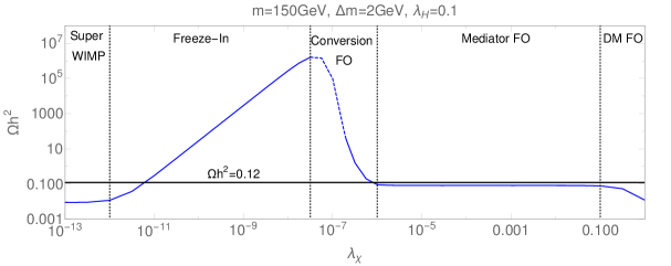
Figure 2: DM abundance as a function of the Yukawa coupling for $m_{\chi}=150$ GeV, $\Delta m=2$ GeV and $\lambda_{H}=0.1$ (i.e. for compressed DM-mediator mass spectrum).

Figure 2 shows the dependence of the DM relic abundance with respect to the Yukawa coupling $\lambda_{\chi}$ in the case of compressed mass spectrum. For illustration, we consider a coupling to $l_{R}=\mu_{R}$ with $m_{\chi}=150$ GeV, $\Delta m=2$ GeV and $\lambda_{H}=0.1$, and we comment on the different regimes of DM production that are realized by varying $\lambda_{\chi}$.

For the largest values of the coupling, that is $\lambda_{\chi}>0.1$, the relic abundance decreases with increasing coupling. This is the well known “standard WIMP behavior” with $\Omega h^{2}\propto 1/\langle\sigma v\rangle_{\chi\chi}$ where $\langle\sigma v\rangle_{\chi\chi}$ denotes the cross-section for the dominant annihilation processes ($\chi\chi\to$ SM SM) with $\langle\sigma v\rangle_{\chi\chi}\propto\lambda_{\chi}^{4}$. In the latter case, the freeze-out is DM annihilation driven meaning that freeze-out occurs when the rate of DM annihilation, initially maintaining DM in equilibrium with the SM bath, becomes smaller than the Hubble rate. More generally, in the standard freeze-out regime (DM in CE), the DM abundance goes as $\Omega h^{2}\propto 1/\langle\sigma v\rangle_{eff}$, with $\langle\sigma v\rangle_{eff}$ defined in Eq. (10). Around $\lambda_{\chi}\sim 0.1$, the $\Omega h^{2}$ curve bends and we enter in the co-annihilation driven regime. In the latter case $\chi\phi\to$ SM SM processes can play the main role with $\langle\sigma v\rangle_{eff}\propto\langle\sigma v\rangle_{\phi\chi}\exp(-x_{f}\Delta m/m_{\chi})$ where $x_{f}\sim 30$ and $\langle\sigma v\rangle_{\phi\chi}\propto\lambda_{\chi}^{2}$. For lower values of the coupling, $10^{-6}\lesssim\lambda_{\chi}\lesssim 0.1$, the relic abundance eventually becomes driven by the rate of mediator annihilations, i.e. $\phi\phi^{\dagger}\to$ SM SM, with $\langle\sigma v\rangle_{eff}\propto\langle\sigma v\rangle_{\phi\phi^{\dagger}}\exp(-2x_{f}\Delta m/m_{\chi})$. The cross-section $\langle\sigma v\rangle_{\phi\phi^{\dagger}}$ mainly depends on the gauge and quartic couplings $g,\lambda_{H}\gg\lambda_{\chi}$ and the DM relic density becomes thus independent of the Yukawa coupling $\lambda_{\chi}$. The blue curve of Fig. 2 turn to a constant and the freeze-out has become mediator annihilation driven. The parameter space for annihilating/co-annihilating WIMP model of Eq. (1) has already been studied in details, see e.g. [31] and references therein.

If chemical equilibrium between the DM and the other species could be maintained for even lower values of $\lambda_{\chi}$ we would expect the relic abundance to stay independent of this parameter. Refs. [3] however pointed out that a new window for dark matter production opens at sufficiently small values of $\lambda_{\chi}$. For suppressed rate of conversion processes, here with $\lambda_{\chi}\lesssim 10^{-6}$, we are left with a dark matter abundance that is larger than in the equilibrium case due to inefficient $\chi\to\phi$ conversions. We enter in the conversion driven freeze-out regime with a relic abundance that is larger than in the DM or mediator annihilation driven regime and that increases again with decreasing $\lambda_{\chi}$. This behavior is due to the rate of conversion processes becoming slower than the Hubble rate. In contrast, in the “standard WIMP” freeze-out, it is the rate of the relevant (co-)annihilation processes that become inefficient.

As it is well known for even lower value of the coupling, $\lambda_{\chi}<10^{-8}$, the dark matter is expected to freeze-in, see e.g. [4]. The dark matter is produced through decays or scatterings of the mediator, i.e. $\Omega h^{2}\propto\lambda^{2}_{\chi}$, but the suppressed coupling $\lambda_{\chi}$ prevents $\chi$ to reach its equilibrium density before it freezes-in. In the latter case, contrarily to the freeze-out, the relic abundance eventually decreases thus with decreasing values of the coupling. Notice that in the freeze-in regime inverse decay/scattering processes giving rise to $\chi\to\phi$ can be neglected, see e.g. [4, 53]. Finally, for couplings $\lambda_{\chi}<10^{-12}$, the relic abundance gets eventually settled through the superWIMP mechanism, see [54, 55, 43]. In the latter case, the DM is produced through the decay of the thermally decoupled mediator (after $\phi$ freezes-out) and $\Omega_{\chi}h^{2}=m_{\chi}/m_{\phi}\,\Omega_{\phi}h^{2}$. In the framework considered here $m_{\chi}/m_{\phi}\approx 1$ and the DM relic abundance is just fixed by the mediator freeze-out. As a result the abundance curve becomes again independent of the conversion factor $\lambda_{\chi}$ and we have $\Omega_{\chi}h^{2}\approx\Omega_{\phi}h^{2}$, ie effectively $\langle\sigma v\rangle_{eff}\approx\langle\sigma v\rangle_{\phi\phi^{\dagger}}$. This regime looks a priori very similar to the mediator annihilation driven freeze-out case. The plateaus in the superWIMP regime ($\lambda_{\chi}<10^{-12}$) and in the mediator annihilation driven freeze-out regime ($10^{-6}\lesssim\lambda_{\chi}\lesssim 0.1$) correspond however to two different values of $\Omega_{\chi}h^{2}$. This is because in the latter case the relevant effective annihilation driving the relic abundance $\langle\sigma v\rangle_{eff}$ gets an extra mass splitting dependent Boltzmann factor ($\exp(-2x_{f}\Delta m/m_{\chi})$) and both the mediator and the DM degrees of freedom have to be taken into account in its computation, see eq. (10).

With the dashed line in Fig. 2 we show the “naive” transition between the conversion driven freeze-out and freeze-in regime that one would obtain using Eqs. (3.1) and (3.1). In this picture, one can compute $\phi$ and $\chi$ abundances assuming that they stay in kinetic equilibrium all the way from standard freeze-out to freeze-in. This is difficult to argue. In Ref. [3], the authors compared the results of the un-integrated Boltzmann equations with the one of Eqs. (3.1) and (3.1). It was shown that even though kinetic equilibrium can not be maintained all along the process of conversion driven freeze-out, the resulting error on the estimation of the relic dark matter was small ($\sim 10\%$). The authors argue that this is due to the thermally coupled mediator eventually decaying to the DM at the time of DM freeze-out actually allowing for the dark matter to inherit back a thermal distribution (or at least close enough to it). For this effect to be relevant, the DM abundance should definitively not be too far higher than the mediator abundance around freeze-out. In Fig. 2, the dashed line starts at $\lambda_{\chi}=2\cdot 10^{-7}$ and denotes the cases when $Y_{\chi}-Y_{\phi}>0.1\times Y_{\chi}$ around the time the abundance of $\chi$ freezes. In the latter case, we assume that we are in the same situation as in [3] and we neglect departure from kinetic equilibrium. We have checked that all viable models considered in the following for conversion driven freeze-out satisfy to this 10% condition.

In what follows we study in more details two benchmark points of Fig. 2 giving rise to $\Omega h^{2}=0.12$ in the regime of conversion driven freeze-out and freeze-in (with a coupling to the SM muon and $m_{\chi}=150$ GeV, $\Delta m=2$ GeV, and $\lambda_{H}=0.1$). For the latter purpose, we compare, for fixed value of $\lambda_{\chi}$, the rates of interaction involved in Eqs. (3.1) and (3.1) to the Hubble rate in Figs 3a and 3c and show the associated evolution of the DM and mediator yields in Figs. 3b and  3d. The plotted rates $\Gamma$ for a given process in Figs. 3a and 3c are taken to be $\Gamma_{ij\to k(l)}=\gamma_{ij\to k(l)}/n^{eq}_{\chi}$, except for the rate of $\phi$ annihilation in which case $\Gamma_{\phi\phi^{\dagger}\to{\rm SM\,SM}}=\gamma_{\phi\phi^{\dagger}}/n^{eq}_{\phi}$. In addition let us emphasize that contrarily to the annihilation driven freeze-out, the DM abundance through freeze-in depends on the initial conditions assumed for $Y_{\chi}$, see e.g. [4]. For conversion driven freeze-out there can be a dependence on the initial conditions as well, see Appendix B for a discussion. All along this paper we assume a negligible initial $\chi$ abundance.

3.2.1 Conversion driven freeze-out

(a)

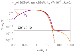
(b)

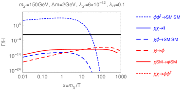
(c)

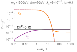
(d)

Figure 3: Benchmark points of Fig. 2 giving rise to $\Omega h^{2}=0.12$. Left: Ratio of the rates of interactions depicted in the legend and of the Hubble rate as a function of $x=\frac{m_{\chi}}{T}$. The conversion processes are depicted in red, the (co-)annihilation ones in blue. The black line depicts $\Gamma/H=1$. Right: Evolution of the yield of $\chi$ (solid purple line) and $\phi$ (solid orange line) and their equilibrium yield (dashed lines) as a function of $x$. Notice that, given the small $\Delta m$ the two equilibrium curves (dashed) are almost indistinguishable.

Within the set up considered in Fig. 2, we obtain $\Omega h^{2}=0.12$ through conversion driven freeze-out for $\lambda_{\chi}=7\cdot 10^{-7}$. The associated rate and abundance evolution are shown in Figs. 3a and 3b. We readily see in Fig. 3b that the $\chi$ population does not follow its equilibrium number density evolution and that before the standard freeze-out temperature (or equivalently $x=m_{\chi}/T\sim 30$) it gives rise to $n_{\chi}(T)>n_{\chi}^{eq}(T)$ due to the suppressed conversion processes that are unable remove the overabundant $\chi$ efficiently.

Considering Fig. 3a, we confirm that we are in a regime in which the most efficient process in reducing the dark sector abundance is the mediator annihilation (short dashed blue line). In contrast, coannihilation (long dashed blue) and especially annihilation processes (continuous blue and short-dashed red) are always suppressed. On the other hand some of the conversion rates can be of the order of, or faster than, the Hubble rate before the mediator freezes-out, as can be seen with the continuous and long-dashed red lines. Those processes will thus affect both the DM and the mediator abundance along the time. For the benchmark model considered here the 4 particles interactions ($\chi$SM$\to\phi$SM) dominate at early times while the 3 particles interaction (inverse mediator decay) play the leading role around the freeze-out time. Given that we have considered $Y_{\chi}=0$ initially, the scatterings $\chi$SM$\to\phi$SM appear to play the most important role in bringing $Y_{\chi}$ near to its equilibrium value at early time. In Fig. 3b, we see that DM yield always deviates from its equilibrium value. It is lower than the equilibrium yield at early time and larger than the equilibrium yield when approaching the freeze-out time. It is also noticeable that when $Y_{\chi}>Y_{\chi}^{eq}$, the DM yield still stays close the its equilibrium yield until the mediator decouples from the thermal bath. This is due to barely but still efficient conversion processes. This behavior has already been described in length in [3]. We discuss further the viable parameter space and detection prospects in the leptophilic scenario in Sec. 4.

3.2.2 Freeze-in from mediator decay and scatterings.

One can also account for all the DM through the freeze-in mechanism for the lowest values of the conversion coupling in Fig. 2, that is $\lambda_{\chi}=6\cdot 10^{-12}$. The associated rates and abundance evolution are shown in Fig. 3c and 3d. In Fig. 3d we mainly recover the standard picture of the dark matter freeze-in which relic abundance is due to scatterings and decays of a mediator in thermodynamic equilibrium with the SM bath. The relic dark matter abundance freezes-in around the time at which the rate of mediator decay/scatterings gets strongly suppressed ($x\sim 3$). Notice that after the mediator freezes-out its relic population eventually decay to DM and leptons at a time characterized by its life-time $\tau_{\phi}$. This would correspond to the “superWIMP” contribution to the relic abundance. For the benchmark considered here $\tau_{\phi}=9s$ which is safely orders of magnitudes below BBN bounds and the superWIMP contribution to the DM relic abundance is around one order of magnitude lower than the freeze-in one. In the rest of this section, we restrict our discussion to the freeze-in contribution to the dark matter relic abundance while neglecting the superWIMP contribution. Note that in Fig. 2 and following sections, the superWIMP contributions have been taken into account. For a detailed study on the freeze-in and superWIMP interplay see e.g. [43].

For reference, we remind that the simplest freeze-in model involves a mother particle $A$ in thermal equilibrium with the SM that decays to a bath particle $B$ and to DM $\chi$. In such a scenario the DM comoving number density induced through freeze-in is associated to the decay only of $A\to B\,\chi$, and the predicted dark matter density simply reduces to [4]:

$$Y_{\chi}=\frac{135g_{A}}{1.66\times 8\pi^{3}g_{*}^{3/2}}\frac{M_{Pl}\Gamma_{A}}{m_{A}^{2}}\,,$$ (13)

where $g_{A}$ counts the spin degrees of freedom of the mother particle $A$, $g_{*}$ is the number of degrees of freedom at the freeze-in temperature $T\sim m_{A}$, and $M_{Pl}=1.22\cdot 10^{19}$ GeV is the Planck mass. This result is however obtained neglecting all potential contributions from scatterings at any time since they are typically sub-dominant compared to the decays [4]. In the case considered here, the equation (13), with the mother particle $A\equiv\phi$, underestimates the relic dark matter abundance in the freeze-in regime. One reason for this is the small mass splitting between the mediator and the DM implying that the decay of the mediator is kinematically suppressed. The contribution to the DM abundance from scattering processes hence becomes more relevant, and this feature is not captured by the simple expression of Eq. (13), see also the discussion in [53].

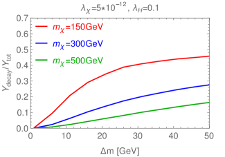
Figure 4: The ratio of the freeze-in yields $Y^{fi}_{\rm decay}/Y^{fi}_{\rm tot}$ as a function of $\Delta m$ when taking only decay processes into account for $Y^{fi}_{\rm decay}$ and including all the relevant scattering and decay processes for $Y_{\rm tot}^{fi}$. We show the results for three different values of the DM mass $m_{\chi}\in\{150,300,500\}$ GeV while keeping $\lambda_{\chi}=5\cdot 10^{-12}$ and $\lambda_{H}=0.1$ fixed.

The relative importance of the decay contribution to the freeze-in is displayed as a function of the mass splitting in Fig. 4. The red curve correspond to an illustrative benchmark with $m_{\chi}=150$ GeV, $\lambda_{\chi}=5\cdot 10^{-12}$ and $\lambda_{H}=0.1$. We show the ratio between the DM abundances obtained through freeze-in $Y^{fi}_{\rm decay}/Y^{fi}_{\rm tot}$ considering the decay processes only for $Y^{fi}_{\rm decay}$ (setting the scattering processes to zero by hand) and including all the relevant scattering and decay processes for $Y_{\rm tot}^{fi}$. For small mass splittings, the mediator decay contribution is subleading. For increasing mass splitting, instead, the decay process becomes the main player. Let us emphasize though that even for the largest values of the mass splitting considered in Fig. 4 the contribution from scattering is non negligible. This is due to the fact that, in the model under study, a large number of scattering processes can contribute to the DM production. There are indeed $\sim$ 10 possible scattering processes with a rate of DM production $\propto\lambda_{\chi}^{2}\alpha$ to be compared to one single decay process with a rate $\propto\lambda_{\chi}^{2}$, where $\alpha$ is the fine structure constant (Tab. 2 in Appendix A lists all the relevant processes). The multiplicity factor of the scattering process partially compensates for the extra SM gauge coupling suppression $\alpha$. As a result, scattering contribution to the dark matter relic abundance through freeze-in can still be $\sim{\cal O}(1)$ compared to the decays for sizeable mass splitting. The relative contribution of the decay is also a function of the mediator mass. The larger the mediator mass, the smaller is the decay contribution at fixed value of the couplings and of the mass spitting (see the blue and green curves in Fig. 4). This is because the decay rate scales like $\Gamma_{\phi}\sim m_{\phi}^{-1}$, see Sec.4.2.

The fact that scatterings can dominate the freeze-in production can also be seen in Fig. 3c, in the case of a freeze-in benchmark scenario with small mass splitting. We indeed see that the scattering processes are more efficient than the decay process for the entire period in which the mediator abundance is unsuppressed. We conclude that both scatterings and decay contribution must be taken into account here to provide a correct estimate of the relic dark matter abundance through freeze-in.

Let us also mention that throughout this paper, we neglect quantum statistical effects and we use the Maxwell Boltzmann equilibrium distributions $f_{i}^{eq}$. Notice however that, when considering the DM production mechanisms for suppressed dark matter couplings and small mass, splittings between the DM and the mediator the precise statistics can be relevant. Taking into account Fermi Dirac statistics for the lepton and DM produced by freeze-in through decay can actually give rise up to a 50% suppression of the DM abundance, see the micrOMEGAs5.0 paper [53] for a discussion. Making use of micrOMEGAs5.0, we have explicitly checked, that for the benchmark model of Fig. 2 the suppression is always $\sim$ 50% in the freeze-in region while, for the typical mass range and mass splittings considered here, the suppression is always between 10 and 50%. Overall we do not expect this effect to qualitatively change the results presented here.

4 Phenomenology of conversion driven freeze-out

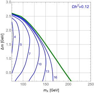
(a) $\lambda_{H}=0.01$

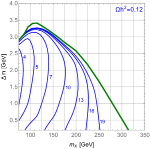
(b) $\lambda_{H}=0.1$

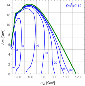
(c) $\lambda_{H}=0.5$

Figure 5: Viable parameter space for DM abundance through conversion driven freeze-out for several value of the $H-\phi$ coupling $\lambda_{H}$. Contours denoting $\Omega h^{2}=0.12$ for fixed value of the Yukawa coupling $\lambda_{\chi}/10^{-7}$ are shown with blue lines. The border of the parameter space is delimited by a green contour corresponding the combinations of $\Delta m,m$ giving rise to the right dark matter abundance through mediator annihilation driven freeze-out.

We focus now on the new region of the parameter space with feeble couplings giving rise to all the DM through the conversion driven freeze-out. This DM production regime opens up for compressed mediator-DM mass spectrum, and suppressed conversion couplings such that the DM is out of CE, as described in Sec. 3.2.1. Notice that the DM freeze-in has been considered in a similar scenario in Ref. [15] while the (co-)annihilation freeze-out has been considered in  [30, 31, 32, 33, 34, 37, 38, 39, 40, 41, 42]. We discuss the viable parameter space (i.e. $\Omega h^{2}=0.12$) for conversion driven freeze-out in Sec. 4.1 and we study the collider constraints in Sec. 4.2.

4.1 Viable parameter space

In the 3 plots of Fig. 5, corresponding to 3 values of the Higgs-mediator coupling $\lambda_{H}$, the viable parameter space for conversion driven freeze-out is enclosed by the green line in the plane $(m_{\chi},\Delta m)$. We readily see that larger values of $\lambda_{H}$ give rise to a larger viable parameter space. Let us first comment on the area above the green contour. In the latter region, the standard freeze-out mechanism (with DM in CE) can give rise to all the DM for a specific choice of the coupling $\lambda_{\chi}$. For large $\Delta m$ or $m_{\chi}$ (above the green line), the freeze-out is DM annihilation driven, i.e. the $\langle\sigma v\rangle_{eff}$ of Eq. (10) is directly given by the dark matter annihilation cross-section $\langle\sigma v\rangle_{\chi\chi}$. Approaching the green line at fixed value of $m_{\chi}$ implies smaller mass splitting $\Delta m$ and thus a larger contribution of co-annihilation processes to $\langle\sigma v\rangle_{eff}$. The green line itself delimiting the viable parameter space for conversion driven freeze-out is obtained by requiring that mediator annihilation driven freeze-out give rise to all the DM (DM still in CE). In the latter case, $\langle\sigma v\rangle_{eff}$ is directly proportional to the mediator annihilation cross section $\langle\sigma v\rangle_{\phi\phi^{\dagger}}$ and to the Boltzmann suppression factor $\exp(-2x_{f}\Delta m/m_{\chi})$ with $x_{f}\approx 30$. Let us emphasize that the green border, in the 2-dimensional $(m_{\chi},\Delta m)$ plane, can be realized for a wide range of suppressed conversion couplings. In e.g. the specific benchmark case of Fig. 2, the mediator driven freeze-out region extended from $\lambda_{\chi}\sim 10^{-1}$ to $\lambda_{\chi}\sim 10^{-6}$ giving rise to a fixed value of $\Omega h^{2}$. Notice that the entire region of the parameter space above the green line has already been analyzed in details in previous studies, see e.g. [31], and we do not further comment on this region here.

Below the green line, the standard freeze-out computation (assuming DM in CE) would predict an underabundant DM population. The conversion coupling gets however so suppressed that the DM can not any more be considered in CE and the standard computation involving Eq. (10) breaks down. In contrast, the treatment of the Boltzmann equations described in Sec. 3.1 can properly follow the DM yield evolution in such a region. As a result the blue contours in Fig. 2 can give rise to $\Omega h^{2}=0.12$ through conversion driven freeze-out (DM out of CE) for fixed value of $\lambda_{\chi}\in$ few $\times[10^{-7},10^{-6}]$.

We also notice that the maximum value of the allowed mass splitting and of the dark matter mass in the conversion driven region increase with the Higgs portal coupling, going from $\Delta m_{max}\simeq 2.6$ GeV and $m_{\chi}^{max}=180$ GeV for the minimal value of $\lambda_{H}=0.01$ to $\Delta m_{max}\simeq 14$ GeV and $m_{\chi}^{max}=1$ TeV for e.g. $\lambda_{H}=0.5$. Increasing $\lambda_{H}$ effectively increases the resulting $\langle\sigma v\rangle_{\rm eff}$ and, as a consequence, decreases the DM relic abundance through mediator annihilation driven freeze-out which is relevant for the extraction of the green contour. In order to understand this behavior let us comment on the overall shape of the viable parameter space delimited by the green line. This line corresponds to models giving $\Omega h^{2}=0.12$ considering mediator annihilation driven freeze-out, i.e. $\langle\sigma v\rangle_{eff}\propto\langle\sigma v\rangle_{\phi\phi^{\dagger}}\exp(-2x_{f}\Delta m/m_{\chi})$ where $\langle\sigma v\rangle_{\phi\phi^{\dagger}}$ mainly depends on $\alpha,\lambda_{H}$. It is easy to check that the general dependence of the countour (hill shape) just results from the competition between the two factors $\langle\sigma v\rangle_{\phi\phi^{\dagger}}$ and $\exp(-2x_{f}\Delta m/m_{\chi})$.

Let us first focus on the large mass range, where the green line display a negative slope in the $(m_{\chi},\Delta m)$ plane. At fixed value of $m_{\chi}$, decreasing $\Delta m$, one decreases $\Omega h^{2}$. This is due to the $\propto\exp(-2x\Delta m/m_{\chi})$ dependence of the annihilation cross-section. One way to compensate for this effect and anyway obtain the correct relic abundance is to consider larger values of the mediator mass (or equivalently the DM mass) as one can expect $\langle\sigma v\rangle_{\phi\phi^{\dagger}}\propto m_{\phi}^{-2}$ for large enough $m_{\phi}$. As a result, for fixed $\Omega h^{2}$, lower $\Delta m$ implies larger $m_{\phi}$. This is indeed the shape of the green line that we recover for large $m_{\phi}$ in the plots of Fig. 5. At some point $\Delta m<m_{l}$ where $l$ is the SM fermion involved in the Yukawa interaction (1) and we get to the maximum allowed value of $m_{\phi}$ (focusing on 2 body decay $\phi\to\chi l$ only). By the same token, one simple way to enlarge the parameter space allowing for larger $m_{\chi}$ at fixed $\Delta m$ is to increase the annihilation rate of the mediator, which can be done by increasing $\lambda_{H}$. Therefore, increasing $\lambda_{H}$ implies a larger viable value of $m_{\phi}$ (or equivalently $m_{\chi}$) to account for the right DM abundance. Going back to the benchmark of Fig. 2, this would imply the horizontal part of the $\Omega h^{2}$ curve goes to lower $\Omega h^{2}$ value when increasing $\lambda_{H}$. This is shown with the red curve of Fig. 8 in appendix A. Also, as illustrated in Fig. 8, this effect can be compensated either by increasing the DM/mediator mass (orange curve in Fig. 8) or by increasing the mass splitting (green curve in Fig. 8) as expected from the green contours of Fig. 5.

Finally, we comment on the shape of the green line in the small mass region, where it has a positive slope in the $(m_{\chi},\Delta m)$ plane. This time this is mainly due to the $\exp(-2x_{f}\Delta m/m_{\chi})$ factor in $\langle\sigma v\rangle_{eff}.$ In the small mass region the exponential suppression is dominant in determining the shape. Larger $\Delta m$ hence requires larger $m_{\chi}$ in order to keep the dark matter abundance at the correct value. Note that this region is present also in the small $\lambda_{H}$ case, but it is realized for dark matter masses lower than the ones showed in the plots (and not phenomenologically interesting, see next section).

4.2 Collider constraints

In this section we discuss the collider constraints on the conversion driven regime. The small Yukawa couplings necessary to reproduce the correct DM relic abundance shown in Fig. 5 (blue contours), together with the mass compression, imply a small decay width of the charged mediator through the process $\phi\rightarrow\chi l$. For $\Delta m\ll m_{\chi}$, the decay rate for $\phi\rightarrow\chi l$ reduces at first orders in $\Delta m$ to:

$$\Gamma_{\phi}\approx\frac{\lambda_{\chi}^{2}\Delta m^{2}}{4\pi m_{\chi}}\left[1-\frac{2\Delta m}{m_{\chi}}\right]\sim\frac{1}{25\text{ cm}}\left(\frac{\lambda_{\chi}}{10^{-6}}\right)^{2}\left(\frac{\Delta m}{1\text{ GeV}}\right)^{2}\left(\frac{100\text{ GeV}}{m_{\chi}}\right)$$ (14)

when neglecting the lepton mass ($m_{l}\ll m_{\chi},m_{\phi}$). The testable signature at colliders for this class of model is hence the pair production of charged mediators through gauge interaction and possibly their subsequent macroscopic decay into DM plus leptons. In the next sections we will discuss in details the possible collider signatures associated to these processes and in particular the expected sensitivity at the LHC. For a recent overview of long-lived particle (LLP) searches see [22].

The overall result of our investigations is shown in Fig. 6 in the mediator proper decay length $c\tau_{\phi}=1/\Gamma_{\phi}$ versus mediator mass plane. The blue contours give rise to $\Omega h^{2}=0.12$ for fixed values of the mass splitting. We consider mediator masses with $m_{\phi}>100$ GeV as charged particles with smaller masses are typically excluded by LEP data [57]. The gray dotted line indicates the region where we go beyond CE regime. Above the gray line the DM abundance can be accounted for through conversion driven freeze-out while below the gray line, mediator annihilation driven freeze-out is at work. In the latter case, the relic abundance become essentially independent of the coupling $\lambda_{\chi}$ and is determined by a combination of the parameters $\lambda_{H},m_{\phi}$ and $\Delta m$. For fixed values of the latter parameters, several values of $\lambda_{\chi}$ (or equivalently $c\tau_{\phi}$ given Eq. (14)) can thus account for the same DM abundance. As a result the blue contours become vertical in the bottom part the plots. Notice that for e.g. $\lambda_{H}=0.5$ case the inverse-$U$-shape of the blue contour at $\Delta m=10$ GeV is to be expected given the form of the blue and green contours of the Fig. 5. In particular the green contours tell us that the right abundance can be obtained at $\Delta m=10$ GeV in the mediator annihilation freeze-out regime for two dark matter masses: $m_{\chi}\approx 150$ and 700 GeV. This is indeed what can be inferred from the lower region of the $\lambda_{H}=0.5$ plot of Fig. 6.

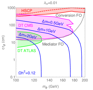
(a) $\lambda_{H}=0.01$

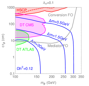
(b) $\lambda_{H}=0.1$

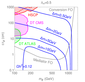
(c) $\lambda_{H}=0.5$

Figure 6: Proper life time of the mediator as a function of the dark matter mass. Each panel corresponds to a different value of $\lambda_{H}$ contributing to the mediator annihilation. The blue contours reproduce the correct relic abundance in the $(m_{\chi},c\tau_{\phi})$ plane for different values of the mass-splitting $\Delta m$. The gray dotted line separates the conversion driven (top) from the mediator annihilation driven (bottom) freeze-out regime. The excluded regions resulting from heavy stable particle (HSCP, red region) searches and disappearing tracks (DT, green region) searches at LHC are also shown. See text for details.

Further constraints can be derived exploiting the long lifetime of the mediator. The charged track limit derived from the Heavy Stable Charged Particle (HSCP) searches of Refs. [58] and [59] are displayed in red in Fig. 6. In Sec. 4.2.1 we describe the detailed derivation of these bounds. For a moderate decay length of the mediator the relevant signature is covered by the disappearing charged tracks (DT) searches since the final state particles (lepton plus dark matter) are not visible in the detector because of the small mass splitting. The purple region shows the region excluded by the CMS analysis [60], while the bound obtained from the ATLAS search [61] is displayed in green. The reinterpretation of these analysis, originally performed for long-lived charginos in supersymmetric models, for our DM model is discussed in Sec. 4.2.2. Note that, as already noticed in e.g. [15], ATLAS and CMS provide a complementary constraints on the lifetime of the mediator.

We comment on displaced leptons searches in Sec. 4.2.3 and on other possibly relevant LHC searches in Sec. 4.2.4. We will see that with those searches we do not get any further constraints on the parameter space of Fig. 6. It is interesting to observe that the current LHC reach on this DM model, even if it includes light charged mediators, is very weak, and a large portion of the parameter space remains unconstrained. We comment on possible strategies to improve the LHC sensitivity along the discussion of the different existing searches.

Finally, let us comment on possible constraints beyond the collider phenomenology. First, we notice that the mediator lifetime is always safely below the BBN constraints, see [56] for an estimation. Furthermore, the leptophilic model considered here with compressed DM-mediator spectrum could potentially give rise to enhanced gamma-ray lines and bremsstrhlung relevant for indirect dark matter searches, direct detection constraints from anapole moment contributions as well as lepton magnetic moment and Lepton flavour violation see e.g. [30, 31, 32, 33, 37, 34]. Even in the WIMP case, only gamma ray constraints and anapole contributions to the DM scattering on nucleon were shown to marginally constrain the DM parameter space, see [34]. In all cases, the relevant observables scale as $\lambda_{\chi}$ to the power 2 or 4 [30, 31, 32, 33]. Given that even smaller dark matter coupling are considered for conversion driven freeze-out, no extra constraints can be extracted.

4.2.1 Charged tracks

One possible avenue to constrain the model under study is to look at charged tracks resulting from pair production of the mediators that are sufficiently long lived to decay outside the detector. In order to reinterpret available analysis within the framework considered here, we have made use of the public code SModelS [62, 63]. This code allows for a decomposition of the collider signature of a given new physics model (within which the stability of the DM is ensured by $Z_{2}$ symmetry) into a sum of simplified-model topologies. SModelS can then use the cross-section upper limits and efficiency maps provided by the experimental collaborations for simplified models and apply them to the new BSM model under study.

We consider the cases in which these topologies are expected to give rise to 2 HSCP in the final state. For the latter purposes, SModelS evaluates the fraction of BSM particles decaying outside the detector ${\cal F}_{long}$. The latter are computed making use of the approximation:

$${\cal F}_{long}=\exp\left(-1\frac{1}{c\tau}\left\langle\frac{l_{out}}{\gamma\beta}\right\rangle_{eff}\right)\,,$$ (15)

where $\beta$ is the velocity of the LLP, $\gamma=(1-\beta^{2})^{-1/2}$, $l_{out}$ is the travel length through the CMS detector (ATLAS analysis are not yet included) and $c\tau$ is the LLP proper decay length. Here we use $\gamma\beta=2.0$ both for our 13 TeV and 8 TeV reinterpretations, see the Appendix C.1 for a discussion motivating such a choice. In addition, we have to provide SModelS with the production cross-sections of our mediator. The production cross section is equivalent to the one of a right handed slepton pair in a SUSY model. We took the NLO+NLL cross sections tabulated by the “LHC SUSY Cross Section Working Group" which have been derived using Resummino [64]. Notice that the latter just simply correspond to the LO cross-sections (that can be obtained with Madgraph) with a $K$-factor correction of roughly $1.5$ at $8$ TeV and $1.3$ at $13$ TeV.

The regions excluded at 95% CL obtained, using efficiency maps, are shown in Fig. 6 with red color. The red dashed curve delimit the 8 TeV exclusion region using the online material provided by the CMS collaboration in CMS-EXO-13-006 [58] while the 13 TeV continuous red contour uses CMS-PAS-EXO-16-036 (with $12.9~{}\mathrm{fb}^{-1}$ data) [59]. Notice that our 8 TeV curve gives rise to slightly less constraining limits than the ones derived in [65] for similar scenario ($\tilde{\tau}$ only) while the 13 TeV ones provide more stringent limit in most of the mass range and extend to larger masses. The 13 TeV data exclude dark matter masses up to $\sim 350$ GeV. Higher mass or equivalently lower production cross-sections can not currently be constrained.

4.2.2 Disappearing tracks

If the decay length of the mediator is still macroscopic but comparable with the typical size of the detector, another interesting collider signature can be considered. In this case, the pair produced mediators travel a certain portion of the detector and then decay into dark matter plus leptons. Hence the signal of such process is characterized by disappearing tracks. Indeed, the dark matter is invisible and, because of the typical small mass splitting, the emitted leptons are too soft to be reconstructed. Similar searches have been performed at 13 TeV by CMS [60] and ATLAS [61, 66], focusing on the case of Wino or Higgsino DM in supersymmetry. In such cases, the lightest chargino and neutralinos are almost degenerate in mass. When the chargino is produced (in pair or in association with another neutralino) it flies for a macroscopic distance in the detector and afterwards decays into the lightest neutralino plus a soft pion. These searches hence target charged tracks leaving some hits in the detector but not reaching the outer part, i.e. disappearing tracks.

Our model, for moderate lifetime of the mediator, gives rise to such signatures at colliders. An important difference with respect to the SUSY case, usually considered in experimental searches, is that in our model the number of produced disappearing tracks per event is always two. This differs with respect to the SUSY case where there can be chargino pair production but also chargino-neutralino associated production.

Here we assess the reach of disappearing track searches on our DM model for both the ATLAS [61] and the CMS [60] search. In the auxiliary HEPData material of the ATLAS search, efficiency maps are provided as a function of the mass of the long-lived charged particle and its lifetime, for the case of electroweak production. In Appendix C, we first make use of these efficiencies to reproduce the exclusion curve of the ATLAS paper for the pure Wino, and we then explain how we derive the corresponding exclusion curve for our DM model. In the auxiliary material of the CMS search, on the other hand, the upper limit cross section as a function of the Wino mass and of its lifetime is reported. In Appendix C we explain how (and under which approximations) we employ this information to derive the corresponding upper limit on our model. Notice that we assume that the efficiencies considered in the ATLAS and CMS analysis respectively also apply to our model. This is because our mediators are produced through electroweak processes, like the Wino. In Fig. 6 we show with a green (purple) region the exclusion limit that we obtain by reinterpreting the ATLAS (CMS) disappearing track search on our model assuming a mass splitting such that the emitted lepton cannot be reconstructed.

4.2.3 Displaced lepton pairs

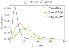
(a)

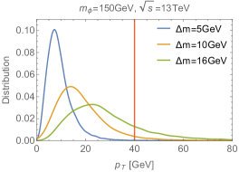
(b)

Figure 7: The $p_{T}$-distribution of the leading muons for the case when $m_{\phi}=$ 150 GeV and different values of the mass splitting. The red vertical line denotes the cut on the $p_{T}$ that is made in the search [67, 68] at 25GeV for $\sqrt{s}=$ 8 TeV (left) and 40 GeV for $\sqrt{s}=$ 13 TeV (right).

There is actually a significant portion of the parameter space where the decay of the charged mediators can occur inside the collider, see Fig. 6. In the latter case, the final topology of the signal includes a pair of displaced leptons and a pair of dark matter particles. If the leptons can be reconstructed, this final state could be constrained by displaced lepton searches [67, 68]. It is important to note that the CMS search [67, 68] targets $e\mu$ final states, while in order to probe our model a search targeting same flavour leptons, as also suggested in [65], would be needed.

Assuming that a same flavour lepton search could be performed, the focus of our study is anyway in the compressed spectrum regime, and hence the leptons will be generically soft and difficult to reconstruct. Note that the missing energy of the process projected in the transverse plane will also be negligible because the compressed mass spectrum implies that the two dark matter particles are mostly produced back to back.

Nevertheless, in order to estimate the possible reach of a displaced lepton search on the parameter space of conversion driven freeze out, we analyze the $p_{T}$ distribution of the produced lepton on few benchmarks. We employ Madgraph [69, 70] to simulate the production of a pair of mediators and their subsequent decay into muon and dark matter. In Fig. 7 we display the $p_{T}$ distribution for the leading muon for three different mass splittings $\Delta m=5,10,16$ GeV. We note that in [67, 68] a minimal $p_{T}$ cut on the outgoing muon is 25 and 40 GeV, respectively at $\sqrt{s}=$ 8 TeV and $\sqrt{s}=$ 13 TeV. We take these as reference value cuts for an hypothetical experimental search looking for same flavour displaced leptons, and we highlight these cuts in Fig. 7 with red vertical lines. From these distributions we conclude that, due to the small mass splitting, most of the events will not pass the minimal cut and therefore these searches will not put any constraints on our model. In this perspective, it would be interesting to explore how much the minimal $p_{T}$ cut on the leptons could be reduced in displaced lepton searches, as also suggested in [16].

4.2.4 Comments on other LHC searches

The difficulties in probing soft objects at the LHC is not only related to their reconstruction, but also to the necessity of triggering on the event. These issues can be typically solved by considering processes accompanied by energetic initial state QCD radiation. In this perspective, relevant searches for our model can be the monojet analysis [71, 72] or the recent boosted soft lepton analysis [73]. However, the latter does not apply to our scenario since it requires soft leptons that are promptly produced.

We can easily provide an estimation of the monojet search bound and conclude that there is not enough sensitivity so as to be relevant for our model. This is principally due to the small electroweak production cross section. As an illustrative case, we considered a benchmark with $m_{\phi}=100$ GeV for which we simulated the pair production of mediators with the addition of one extra energetic jet using Madgraph. The signal region categories of [71] starts at $E^{miss}_{T}>$ 250 GeV and put 95% CL on the visible cross section in several bins with increasing $E^{miss}_{T}$ cuts. We have verified that, once an extra jet with the corresponding $p_{T}$ is required, the cross section in our model is always at least two order of magnitudes below the experimentally excluded cross section in all the $E^{miss}_{T}$ bins. Hence we conclude that monojet searches can not constraint the parameter space of our model.

5 Conclusions

The main goal of the paper is to determine the viable parameter space and the associated experimental constraints for a dark matter candidate that account for all the dark matter when produced at early times through conversion driven freeze-out, i.e. investigating the dark matter freeze-out beyond CE. We have worked in a simplified model including a Majorana dark matter fermion $\chi$ coupling to SM lepton and a charged dark scalar $\phi$, the mediator, through a Yukawa coupling. The minimal set of extra parameters for this model are the Yukawa coupling $\lambda_{\chi}$, responsible for the conversion processes, the dark matter mass $m_{\chi}$ and the mass splitting between the mediator and the DM $\Delta m$. In addition, given that the mediator is a charged scalar, one can always write a quartic interactions between $\phi$ and the Higgs driven by the coupling $\lambda_{H}$. We have considered a few benchmark values of the latter coupling for illustration. The parameter space studied here involves relatively feeble conversion couplings $\lambda_{\chi}$ compared to previous analysis made within the context of the WIMP paradigm [30, 31, 32, 33, 37, 34] and extend the conversion driven analysis [3, 5] to the case of a leptophilic scenario.

As a first step, we have described how varying the conversion coupling one can continuously go from DM annihilation driven freeze-out to freeze-in passing through mediator annihilation and conversion driven freeze-out in the context of compressed mass spectrum. Our discussion is summarized in Fig. 2. We have then focused on the case of conversion driven freeze-out. We have first determined the viable parameter space in order to account for all the DM that typically involves conversion couplings in the range $\lambda_{\chi}\in[10^{-7},10^{-6}]$. For negligible $H$-$\phi$ coupling $\lambda_{H}=0.01$, the latter reduces to a limited parameter space with $m_{\chi}<200$ GeV and $\Delta m<2.6$ GeV. Larger $\lambda_{H}$ increase the mediator annihilation cross-section and, by the same token, extend the viable parameter space to e.g. $m_{\chi}<1$ TeV and $\Delta m<14$ GeV for $\lambda_{H}=0.5$ GeV. The precise viable parameter space is shown Fig. 5 for a selection of $\lambda_{H}$ coupling.

Finally we have addressed the collider constraints on the model under study. Interestingly the feeble coupling involved give rise to a long lived mediator that can a priori be tested through existing searches for heavy stable charged particles, disappearing charged tracks and, possibly, displaced leptons. We have recasted existing searches and projected the results within our scenario as shown in Fig. 6. As can be seen, only disappearing charged tracks and heavy stable charged particle searches provide relevant constraints on the parameter space. We also explicitly checked that displaced leptons and monojet searches can not help to further test our DM scenario. At this point, a large part of the parameter space is left unconstrained.

Appendix A Relevant processes for the Relic abundance computation

In table 1 and 2, all the processes that influence the relic abundance are summarized. All of them have a different influence and therefore, we compare all the relevant rates of interaction to the Hubble rate. If $\Gamma>H$, they are efficient and the interactions happen fast enough such that the process is in equilibrium. The rates used in Fig. 3a and 3c are defined as $\Gamma_{ij\to k(l)}=\gamma_{ij\to k(l)}/n^{eq}_{\chi}$, except for the rate of $\phi$ annihilation in which case $\Gamma_{\phi\phi^{\dagger}\to{\rm SM\,SM}}=\gamma_{\phi\phi^{\dagger}}/n^{eq}_{\phi}$. If one compares the rates in Fig. 3a and 3c with tables 1 and 2, one can spot that there is one process missing, namely $\phi\phi\rightarrow ll$. This process has the same influence as $\phi\phi^{\dagger}\rightarrow SMSM$ on the relic abundance, but it is suppressed by $\lambda_{\chi}^{4}$. It is always sub-leading (unless $\lambda_{\chi}\approx 1$, a regime we are not interested in) and therefore, it is not included in the plots where we compare the efficiencies of the different rates or in the Boltzmann equation.
The decay rate for $\phi\rightarrow\chi l$ (not thermally averaged!) reads

$$\Gamma_{\phi} =\lambda_{\chi}^{2}\frac{(m_{\phi}^{2}-m_{l}^{2}-m_{\chi}^{2})\sqrt{\left[m_{\phi}^{2}-(m_{\chi}-m_{l})^{2}\right]\left[m_{\phi}^{2}-(m_{\chi}+m_{l})^{2}\right]}}{16\pi m_{\phi}^{3}},$$ (16)

$$\approx\frac{\lambda_{\chi}^{2}\Delta m^{2}}{4\pi m_{\chi}}\left[1-\frac{2\Delta m}{m_{\chi}}+\dots\right],$$ (17)

where in the second line we have assumed small mass splittings ($\Delta m\ll m$) and we have neglected the lepton mass. The cross-sections have been obtained making use of FeynRules [51] and Calchep[52] to extract the transition amplitudes $\mathcal{M}$ as:

$$\langle\sigma_{ij}v\rangle n_{i,eq}n_{j,eq}=\frac{g_{i}g_{j}}{512\pi^{5}}T\int\frac{|\mathcal{M}|^{2}}{\sqrt{s}}K_{1}\left(\frac{\sqrt{s}}{T}\right)ds\ dt,$$ (18)

with

$$n_{i,eq}=\frac{g_{i}}{2\pi^{2}}m_{i}^{2}TK_{2}(m_{i}/T),$$ (19)

where $K_{1,2}$ are the first and second modified Bessel functions of the 2nd kind. In some of the above cases, some $s-$ and $t-$channel divergences can appear. In the latter cases, we follow the same procedure as in [3] introducing cuts in the integration regions to handle them. We checked that our results were stable varying the cuts.

initial state		final state		scaling with $\lambda_{\chi}$
$\chi$	$\chi$	$l^{-}$	$l^{+}$	$\lambda_{\chi}^{4}$
$\chi$	$\phi$	$l^{-}$	$\gamma,Z,H$	$\lambda_{\chi}^{2}$
		$W^{-}$	$\nu_{l}$
$\phi$	$\phi^{\dagger}$	$\gamma,Z,W^{+}$	$\gamma,Z,W^{-}$	$\lambda_{\chi}^{0}$
		$q$	$\bar{q}$
		$H$	$Z,H$
		$l^{-}$	$l^{+}$
$\phi$	$\phi$	$l^{-}$	$l^{-}$	$\lambda_{\chi}^{4}$

Table 1: List of all relevant (co-)annihilation processes. The leptons involved are denoted by $l=e,\mu,\tau$. Also the dependence of the cross section on the coupling constant $\lambda_{\chi}$ is denoted in the last column. The $\phi\phi^{\dagger}$ annihilation into $l\bar{l}$ also has contributions scaling with $\lambda_{\chi}^{2}$ and $\lambda_{\chi}^{4}$.

initial state		final state		scaling
$\chi$	$l^{-}$	$\phi$	$\gamma,Z,H$	$\lambda_{\chi}^{2}$
	$\gamma,Z,H$		$l^{+}$
	$W^{-}$		$\bar{\nu_{l}}$
	$\nu_{l}$		$W^{+}$
$\phi$		$\chi$	$l^{-}$	$\lambda_{\chi}^{2}$
$\chi$	$\chi$	$\phi$	$\phi^{\dagger}$	$\lambda_{\chi}^{4}$

Table 2: List of all included conversion processes and their dependence of the cross section on $\lambda_{\chi}$. $l$ is one of the leptons ($e,\mu,\tau$), depending on the case we are studying.

Finally, when discussing the dependence of the relic abundance on the conversion coupling we looked at a particular benchmark with a coupling to the SM muon and $m_{\chi}=150$ GeV, $\Delta m=2$ GeV, and $\lambda_{H}=0.1$. The latter case was shown in Fig. 2. For the sake of illustration we also show how the $\Omega h^{2}$ curve is affected varying $m_{\chi}$, $\Delta m$, and $\lambda_{H}$ in Fig. 8, see also the discussion in Sec. 4.

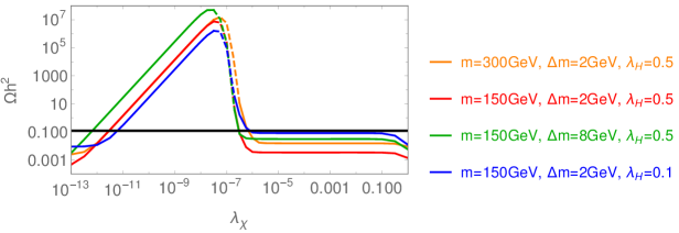
Figure 8: DM abundance as a function of the Yukawa coupling (as in Fig. 2) for different values of the parameters $m_{\chi}$, $\Delta m$ and $\lambda_{H}$

Appendix B Dependence on initial conditions

A very interesting feature of the freeze-out mechanism is that it does not depend on the initial conditions. For small values of $x$ ($x\lesssim 1$), the annihilation rates are efficient and therefore, the yield always converges to the equilibrium value, regardless whether we start with zero or with a very high abundance. Instead, in the case of small coupling involved, as the freeze-in case, it is well known that the final DM abundance can be sensitive to the initial conditions (IC). In [3], it was pointed out that when DM couples to light quarks through Eq. (1), the conversion driven abundance is independent of the IC. In contrast, in the case of a coupling to leptons considered here, we clearly notice a dependence on the IC, especially for values of $\lambda_{\chi}\sim\mathcal{O}(10^{-7})$ or less. This is illustrated in Fig. 9 where we show the yields for 2 distinct values of the Yukawa coupling. The reason for this dependence in the leptophilic case is due to the fact that conversion driven processes are less efficient than in the quark-philic case as the gauge coupling involved in the processes depicted in Fig. 1 is the EW coupling instead of strong coupling. In the follow-up we will always assume that $Y_{\chi}(0.01)=0$.

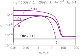
(a) $\lambda_{\chi}=4\cdot 10^{-7}$

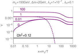
(b) $\lambda_{\chi}=10^{-7}$

Figure 9: Plotting the evolution of the yield for different initial conditions: $Y_{\chi}[1]=i\cdot Y_{\chi,eq}$[1] with $i\in\{0,0.01,1,100\}$. Both figures are calculated with $\widetilde{\mu}$ as the co-annihilation partner and for the parameters $m_{\chi}=150$ GeV and $\Delta m=2$ GeV but for two different values of the coupling, $\lambda_{\chi}=4\cdot 10^{-7}$ (left) and $\lambda_{\chi}=10^{-7}$ (right). The dashed lines denote the equilibrium yield.

Appendix C Technical details on the collider searches

C.1 Charged Tracks

A priori, the evaluation of ${\cal F}_{long}$ in Eq. (15) would require an event-based computation of $l_{out}/\gamma\beta$. In the appendix of [13], it is however argued that considering the effective length $L_{eff}=\left\langle{l_{out}}/{\gamma\beta}\right\rangle_{eff}=7m$ provide conservative constraints. This $L_{eff}$ corresponds to a typical $\gamma\beta\simeq 1.43$ for $l_{out}\simeq 10$ m and is encoded by default in the SModelS code. A closer look to their figure B.6. (in the case of the LLP direct production that we consider here) already tells you that in the mass range of a few hundred of GeV LLP mass, this $\gamma\beta\simeq 1.43$ give rise to a weaker constraint on the LLP life time than in the event-based computation. Making use of our own Madgraph simulations we obtain that the resulting $\gamma\beta$ distribution tends to values larger than 1.43. In particular for a mediator mass between 100 and 250 (100 and 350) GeV, we obtain a mean $\gamma\beta$ varying between 3.5 and 2.0 (4.9 and 2.17) for $\sqrt{s}=8$ TeV (13 TeV). As a result, here we use the conservative value of $\gamma\beta=2.0$ (or equivalently $L_{eff}=5$ m) for our analysis.

C.2 Disappearing Tracks

ATLAS Search

The ATLAS search [61] for events with at least one disappearing track focussed on the case of wino DM. In these supersymmetric models, the lightest chargino and neutralino are almost pure wino and they are nearly mass degenerate. Therefore, the chargino can decay to a neutralino and a soft pion inside the detector, leaving a disappearing track. The ATLAS collaboration provided the efficiency maps for this search in the HEPData. In order to use these efficiency maps to asses the reach of disappearing track searches on our DM model, we need to know how to interpret them.
Besides the event acceptance $E_{A}$ and efficiency $E_{E}$, the tracklet too has to pass the reconstruction selection requirements. The probability to pass the generator-level requirements is the tracklet acceptance $T_{A}$. The probability to pass the full pixel tracklet selection at reconstruction level is the tracklet efficiency $T_{E}$. Both should be applied for every tracklet. Finally, the probability for a tracklet to have a $p_{T}>100GeV$ is denoted independently by $P$ and is taken to have a constant value of 0.57 for the charginos.
There are three different processes that can leave a disappearing track in the detector for the wino-like chargino/neutralino model,

$$pp\rightarrow\chi^{+}_{1}\chi^{-}_{1},$$ (20)

$$pp\rightarrow\chi^{+}_{1}\chi^{0}_{1},$$ (21)

$$pp\rightarrow\chi^{-}_{1}\chi^{0}_{1},$$ (22)

with each of the processes having approximately the same production cross section, i.e. one third of the total cross section. The efficiency map provided in the HEPData denotes the total model dependent efficiency (i.e. taking into account the fact that some of the above processes can leave two tracks in the detector), without taking into account the probability $P$ (it will be reintroduced later). Since in our model, we have only processes that can leave two tracks, we need to obtain the efficiency for two tracklet processes.
In general, the probability $\mathcal{E}_{N}$ of reconstructing at least one tracklet coming from a process leaving $N$ tracks in the detector has an efficiency of,

$$\mathcal{E}_{N} =E_{A}\times E_{E}\times(1-(1-T_{A}\times T_{E})^{N})$$

$$\approx E_{A}\times E_{E}\times(1-(1-N\,T_{A}\times T_{E}))$$

$$=NE_{A}\times E_{E}\times T_{A}\times T_{E}$$

$$=N\mathcal{E}_{1}.$$ (23)

For the wino-like chargino/neutralino analysis, only process (20) can leave two tracks in the detector while the other two can only leave one. Therefore, the model dependent efficiency for the pure wino chargino/neutralino analysis is

$$\mathcal{E}_{full}=\frac{2}{3}\mathcal{E}_{1}+\frac{1}{3}\mathcal{E}_{2}\approx\frac{4}{3}\mathcal{E}_{1}\approx\frac{2}{3}\mathcal{E}_{2},$$ (24)

where the $2/3$ represents the contribution from the processes with one tracklet (i.e. (21) and (22)) and the $1/3$ represents the contribution from the processes with two tracklets (20), all assumed to have the same production cross section. As mentioned, the full efficiency $\mathcal{E}_{full}$ is the one reported in the HEPData and we use Eq. (23) and (24) to derive the efficiency for a two tracklet process, that we use in the analysis of our DM model.
In order to validate this technique, we reproduce the exclusion limit at 95% CL for the pure wino case [61] in figure 10, by multiplying the full efficiency with the total cross-section, together with the probability $P$, to get the visible cross-section.

CMS Search

The CMS search for disappearing tracks [60] focuses on the same model as the ATLAS search, i.e. wino DM. In the HEPData, they provide a 95% CL upper limit $\sigma_{Wino}^{UL}$ on the product of the cross section for direct production of charginos as a function of chargino mass and lifetime. Since this is a model dependent limit, we have to recast this upper limit to account for the fact that for the model under study here, we will always produce two charged tracks in the detector. In order to accommodate this in our analysis, we will make use of the same approximations as for the ATLAS search, namely that the efficiency used for the search can be approximated by Eq. (24). Together with this approximation, we can obtain a 95% CL exclusion limit on the charged scalar $\phi$ in the model under study here from the data given on the HEPData page of the experiment as follows

$$\sigma_{\phi}^{UL}=\frac{\sigma_{vis}^{UL}}{\mathcal{E}_{2}}\approx\frac{2}{3}\frac{\sigma_{vis}^{UL}}{\mathcal{E}_{full}}=\frac{2}{3}\sigma_{Wino}^{UL}.$$ (25)

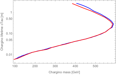
Figure 10: Exclusion limit at 95% CL for the supersymetric pure-wino chargino/neutralino analysis obtained from ref. [61] (red) and by using the recasting of the efficiencies as explained in the text (blue).

References

- [1] X. Chu, T. Hambye and M. H. G. Tytgat, The Four Basic Ways of Creating Dark Matter Through a Portal, JCAP 1205 (2012) 034 [1112.0493].
- [2] N. Bernal, M. Heikinheimo, T. Tenkanen, K. Tuominen and V. Vaskonen, The Dawn of FIMP Dark Matter: A Review of Models and Constraints, Int. J. Mod. Phys. A32 (2017) 1730023 [1706.07442].
- [3] M. Garny, J. Heisig, B. Lulf and S. Vogl, Coannihilation without chemical equilibrium, Phys. Rev. D96 (2017) 103521 [1705.09292].
- [4] L. J. Hall, K. Jedamzik, J. March-Russell and S. M. West, Freeze-In Production of FIMP Dark Matter, JHEP 03 (2010) 080 [0911.1120].
- [5] M. Garny, J. Heisig, M. Hufnagel and B. Lulf, Top-philic dark matter within and beyond the WIMP paradigm, Phys. Rev. D97 (2018) 075002 [1802.00814].
- [6] M. Garny, J. Heisig, M. Hufnagel, B. Lülf and S. Vogl, Conversion-driven freeze-out: Dark matter genesis beyond the WIMP paradigm, in 18th Hellenic School and Workshops on Elementary Particle Physics and Gravity (CORFU2018) Corfu, Corfu, Greece, August 31-September 28, 2018, 2019, 1904.00238.
- [7] D. Abercrombie et al., Dark Matter Benchmark Models for Early LHC Run-2 Searches: Report of the ATLAS/CMS Dark Matter Forum, 1507.00966.
- [8] R. T. Co, F. D’Eramo, L. J. Hall and D. Pappadopulo, Freeze-In Dark Matter with Displaced Signatures at Colliders, JCAP 1512 (2015) 024 [1506.07532].
- [9] A. G. Hessler, A. Ibarra, E. Molinaro and S. Vogl, Probing the scotogenic FIMP at the LHC, JHEP 01 (2017) 100 [1611.09540].
- [10] F. D’Eramo, N. Fernandez and S. Profumo, Dark Matter Freeze-in Production in Fast-Expanding Universes, JCAP 1802 (2018) 046 [1712.07453].
- [11] A. Davoli, A. De Simone, T. Jacques and V. Sanz, Displaced Vertices from Pseudo-Dirac Dark Matter, JHEP 11 (2017) 025 [1706.08985].
- [12] L. Calibbi, L. Lopez-Honorez, S. Lowette and A. Mariotti, Singlet-Doublet Dark Matter Freeze-in: LHC displaced signatures versus cosmology, JHEP 09 (2018) 037 [1805.04423].
- [13] J. Heisig, S. Kraml and A. Lessa, Constraining new physics with searches for long-lived particles: Implementation into SModelS, Phys. Lett. B788 (2019) 87 [1808.05229].
- [14] G. Brooijmans et al., Les Houches 2017: Physics at TeV Colliders New Physics Working Group Report, in 10th Les Houches Workshop on Physics at TeV Colliders (PhysTeV 2017) Les Houches, France, June 5-23, 2017, 2018, 1803.10379, http://lss.fnal.gov/archive/2017/conf/fermilab-conf-17-664-ppd.pdf.
- [15] G. Belanger et al., LHC-friendly minimal freeze-in models, JHEP 02 (2019) 186 [1811.05478].
- [16] A. Filimonova and S. Westhoff, Long live the Higgs portal!, JHEP 02 (2019) 140 [1812.04628].
- [17] J. Heisig, Dark matter and long-lived particles at the LHC, in 53rd Rencontres de Moriond on Electroweak Interactions and Unified Theories (Moriond EW 2018) La Thuile, Italy, March 10-17, 2018, 2018, 1805.07361.
- [18] S. Chang and M. A. Luty, Displaced Dark Matter at Colliders, 0906.5013.
- [19] O. Buchmueller, A. De Roeck, K. Hahn, M. McCullough, P. Schwaller, K. Sung et al., Simplified Models for Displaced Dark Matter Signatures, JHEP 09 (2017) 076 [1704.06515].
- [20] A. Ghosh, T. Mondal and B. Mukhopadhyaya, Heavy stable charged tracks as signatures of non-thermal dark matter at the LHC : a study in some non-supersymmetric scenarios, JHEP 12 (2017) 136 [1706.06815].
- [21] A. Davoli, A. De Simone, T. Jacques and A. Morandini, LHC Phenomenology of Dark Matter with a Color-Octet Partner, 1803.02861.
- [22] J. Alimena et al., Searching for long-lived particles beyond the Standard Model at the Large Hadron Collider, 1903.04497.
- [23] X. Chu, C. Garcia-Cely and T. Hambye, Can the relic density of self-interacting dark matter be due to annihilations into Standard Model particles?, JHEP 11 (2016) 048 [1609.00399].
- [24] N. Bernal, X. Chu, C. Garcia-Cely, T. Hambye and B. Zaldivar, Production Regimes for Self-Interacting Dark Matter, JCAP 1603 (2016) 018 [1510.08063].
- [25] Y. Hochberg, Y. Kahn, M. Lisanti, K. M. Zurek, A. G. Grushin, R. Ilan et al., Detection of sub-MeV Dark Matter with Three-Dimensional Dirac Materials, Phys. Rev. D97 (2018) 015004 [1708.08929].
- [26] S. Knapen, T. Lin, M. Pyle and K. M. Zurek, Detection of Light Dark Matter With Optical Phonons in Polar Materials, 1712.06598.
- [27] M. Heikinheimo, T. Tenkanen and K. Tuominen, Prospects for indirect detection of frozen-in dark matter, Phys. Rev. D97 (2018) 063002 [1801.03089].
- [28] N. Bernal, C. Cosme and T. Tenkanen, Phenomenology of Self-Interacting Dark Matter in a Matter-Dominated Universe, 1803.08064.
- [29] T. Hambye, M. H. G. Tytgat, J. Vandecasteele and L. Vanderheyden, Dark matter direct detection is testing freeze-in, Phys. Rev. D98 (2018) 075017 [1807.05022].
- [30] M. Garny, A. Ibarra and S. Vogl, Dark matter annihilations into two light fermions and one gauge boson: General analysis and antiproton constraints, JCAP 1204 (2012) 033 [1112.5155].
- [31] M. Garny, A. Ibarra and S. Vogl, Signatures of Majorana dark matter with t-channel mediators, Int. J. Mod. Phys. D24 (2015) 1530019 [1503.01500].
- [32] M. Garny, A. Ibarra, M. Pato and S. Vogl, Internal bremsstrahlung signatures in light of direct dark matter searches, JCAP 1312 (2013) 046 [1306.6342].
- [33] T. Bringmann, X. Huang, A. Ibarra, S. Vogl and C. Weniger, Fermi LAT Search for Internal Bremsstrahlung Signatures from Dark Matter Annihilation, JCAP 1207 (2012) 054 [1203.1312].
- [34] J. Kopp, L. Michaels and J. Smirnov, Loopy Constraints on Leptophilic Dark Matter and Internal Bremsstrahlung, JCAP 1404 (2014) 022 [1401.6457].
- [35] M. J. Baker and A. Thamm, Leptonic WIMP Coannihilation and the Current Dark Matter Search Strategy, JHEP 10 (2018) 187 [1806.07896].
- [36] V. V. Khoze, A. D. Plascencia and K. Sakurai, Simplified models of dark matter with a long-lived co-annihilation partner, JHEP 06 (2017) 041 [1702.00750].
- [37] F. Giacchino, L. Lopez-Honorez and M. H. G. Tytgat, Scalar Dark Matter Models with Significant Internal Bremsstrahlung, JCAP 1310 (2013) 025 [1307.6480].
- [38] F. Giacchino, L. Lopez-Honorez and M. H. G. Tytgat, Bremsstrahlung and Gamma Ray Lines in 3 Scenarios of Dark Matter Annihilation, JCAP 1408 (2014) 046 [1405.6921].
- [39] F. Giacchino, A. Ibarra, L. Lopez Honorez, M. H. G. Tytgat and S. Wild, Signatures from Scalar Dark Matter with a Vector-like Quark Mediator, JCAP 1602 (2016) 002 [1511.04452].
- [40] S. Colucci, B. Fuks, F. Giacchino, L. Lopez Honorez, M. H. G. Tytgat and J. Vandecasteele, Top-philic Vector-Like Portal to Scalar Dark Matter, Phys. Rev. D98 (2018) 035002 [1804.05068].
- [41] T. Toma, Internal Bremsstrahlung Signature of Real Scalar Dark Matter and Consistency with Thermal Relic Density, Phys. Rev. Lett. 111 (2013) 091301 [1307.6181].
- [42] A. Ibarra, T. Toma, M. Totzauer and S. Wild, Sharp Gamma-ray Spectral Features from Scalar Dark Matter Annihilations, Phys. Rev. D90 (2014) 043526 [1405.6917].
- [43] M. Garny and J. Heisig, Interplay of super-WIMP and freeze-in production of dark matter, Phys. Rev. D98 (2018) 095031 [1809.10135].
- [44] A. Aboubrahim and P. Nath, Detecting hidden sector dark matter at HL-LHC and HE-LHC via long-lived stau decays, Phys. Rev. D99 (2019) 055037 [1902.05538].
- [45] J. L. Evans, D. E. Morrissey and J. D. Wells, Higgs boson exempt no-scale supersymmetry and its collider and cosmology implications, Phys. Rev. D75 (2007) 055017 [hep-ph/0611185].
- [46] L. Calibbi, A. Mariotti, C. Petersson and D. Redigolo, Selectron NLSP in Gauge Mediation, JHEP 09 (2014) 133 [1405.4859].
- [47] K. Griest and D. Seckel, Three exceptions in the calculation of relic abundances, Phys. Rev. D43 (1991) 3191.
- [48] Planck collaboration, Planck 2015 results. XIII. Cosmological parameters, Astron. Astrophys. 594 (2016) A13 [1502.01589].
- [49] M. A. Luty, Baryogenesis via leptogenesis, Phys. Rev. D 45 (1992) 455.
- [50] M. Frigerio, T. Hambye and E. Masso, Sub-GeV dark matter as pseudo-Goldstone from the seesaw scale, Phys. Rev. X1 (2011) 021026 [1107.4564].
- [51] A. Alloul, N. D. Christensen, C. Degrande, C. Duhr and B. Fuks, FeynRules 2.0 - A complete toolbox for tree-level phenomenology, Comput. Phys. Commun. 185 (2014) 2250 [1310.1921].
- [52] A. Belyaev, N. D. Christensen and A. Pukhov, CalcHEP 3.4 for collider physics within and beyond the Standard Model, Comput. Phys. Commun. 184 (2013) 1729 [1207.6082].
- [53] G. Belanger, F. Boudjema, A. Goudelis, A. Pukhov and B. Zaldivar, micrOMEGAs5.0 : freeze-in, 1801.03509.
- [54] L. Covi, J. E. Kim and L. Roszkowski, Axinos as cold dark matter, Phys. Rev. Lett. 82 (1999) 4180 [hep-ph/9905212].
- [55] J. L. Feng, A. Rajaraman and F. Takayama, SuperWIMP dark matter signals from the early universe, Phys. Rev. D68 (2003) 063504 [hep-ph/0306024].
- [56] K. Jedamzik, Big bang nucleosynthesis constraints on hadronically and electromagnetically decaying relic neutral particles, Phys. Rev. D74 (2006) 103509 [hep-ph/0604251].
- [57] OPAL collaboration, Searches for gauge-mediated supersymmetry breaking topologies in e+ e- collisions at LEP2, Eur. Phys. J. C46 (2006) 307 [hep-ex/0507048].
- [58] CMS collaboration, Constraints on the pMSSM, AMSB model and on other models from the search for long-lived charged particles in proton-proton collisions at sqrt(s) = 8 TeV, Eur. Phys. J. C75 (2015) 325 [1502.02522].
- [59] CMS collaboration, Search for heavy stable charged particles with of 2016 data, .
- [60] CMS collaboration, Search for disappearing tracks as a signature of new long-lived particles in proton-proton collisions at 13 TeV, 1804.07321.
- [61] ATLAS collaboration, Search for long-lived charginos based on a disappearing-track signature in pp collisions at TeV with the ATLAS detector, JHEP 06 (2018) 022 [1712.02118].
- [62] S. Kraml, S. Kulkarni, U. Laa, A. Lessa, W. Magerl, D. Proschofsky-Spindler et al., SModelS: a tool for interpreting simplified-model results from the LHC and its application to supersymmetry, Eur. Phys. J. C74 (2014) 2868 [1312.4175].
- [63] F. Ambrogi et al., SModelS v1.2: long-lived particles, combination of signal regions, and other novelties, 1811.10624.
- [64] B. Fuks, M. Klasen, D. R. Lamprea and M. Rothering, Revisiting slepton pair production at the Large Hadron Collider, JHEP 01 (2014) 168 [1310.2621].
- [65] J. A. Evans and J. Shelton, Long-Lived Staus and Displaced Leptons at the LHC, JHEP 04 (2016) 056 [1601.01326].
- [66] ATLAS Collaboration collaboration, Search for direct pair production of higgsinos by the reinterpretation of the disappearing track analysis with 36.1 fb-1 of TeV data collected with the ATLAS experiment, Tech. Rep. ATL-PHYS-PUB-2017-019, CERN, Geneva, Dec, 2017.
- [67] CMS collaboration, Search for Displaced Supersymmetry in events with an electron and a muon with large impact parameters, Phys. Rev. Lett. 114 (2015) 061801 [1409.4789].
- [68] CMS collaboration, Search for displaced leptons in the e-mu channel, CMS-PAS-EXO-16-022.
- [69] J. Alwall, R. Frederix, S. Frixione, V. Hirschi, F. Maltoni, O. Mattelaer et al., The automated computation of tree-level and next-to-leading order differential cross sections, and their matching to parton shower simulations, JHEP 07 (2014) 079 [1405.0301].
- [70] J. Alwall, M. Herquet, F. Maltoni, O. Mattelaer and T. Stelzer, MadGraph 5 : Going Beyond, JHEP 06 (2011) 128 [1106.0522].
- [71] ATLAS collaboration, Search for dark matter and other new phenomena in events with an energetic jet and large missing transverse momentum using the ATLAS detector, JHEP 01 (2018) 126 [1711.03301].
- [72] CMS collaboration, Search for dark matter produced with an energetic jet or a hadronically decaying W or Z boson at TeV, JHEP 07 (2017) 014 [1703.01651].
- [73] ATLAS collaboration, Search for electroweak production of supersymmetric states in scenarios with compressed mass spectra at TeV with the ATLAS detector, Phys. Rev. D97 (2018) 052010 [1712.08119].